+ All Categories
Home > Documents > A Two-Stage Model of Interacting Producers

A Two-Stage Model of Interacting Producers

Date post: 22-Jan-2022
Category:
Upload: others
View: 1 times
Download: 0 times
Share this document with a friend
152
A Mathematical Programming-Based Analysis of A Two-Stage Model of Interacting Producers by Joanna M. Leleno Dissertation submitted to the Faculty of the Virginia Polytechnic Institute and State University in partial fulfillment of the requirements for the degree of Doctor of Philosophy in Industrial Engineering and Operations Research APPROVED: HanifQ. Sherali, . I If Faiz A. Catherine C. Eckel '14 b G- -·-- K Joel A. Nachlas July 1987 Blacksburg, Virginia
Transcript

A Mathematical Programming-Based Analysis of

A Two-Stage Model of Interacting Producers

by

Joanna M. Leleno

Dissertation submitted to the Faculty of the

Virginia Polytechnic Institute and State University

in partial fulfillment of the requirements for the degree of

Doctor of Philosophy

in

Industrial Engineering and Operations Research

APPROVED:

HanifQ. Sherali, Ch1airma~ .

I If Faiz A. Al-K~#fj Catherine C. Eckel

'14 b G- -·-- K

Joel A. Nachlas

July 1987

Blacksburg, Virginia

A Mathematical Programming-Based Analysis of

A Two-Stage Model of Interacting Producers

by

Joanna M. Leleno

Hanif D. Sherali, Chairman

Industrial Engineering and Operations Research

(ABSTRACT)

This dissertation is concerned with the characterization, existence and computation of equi-

librium solutions in a two-stage model of interacting producers. The model represents an in-

dustry involved with two major stages of production. On the production side there exist some

(upstream) firms which perform the first stage of production and manufacture a semi-finished

product, and there exist some other (downstream) firms which perform the second stage of

production and convert this semi-finished product to a final commodity. There also exist some

(vertically integrated) firms which handle the entire production process themselves.

In this research, the final commodity market is an oligopoly which may exhibit one of two

possible behavioral patterns: follower-follower or multiple leader-follower. In both cases, the

downstream firms are assumed to be price takers in purchasing the intermediate product.

For the upstream stage, we consider two situations: a Cournot oligopoly or a perfectly com-

petitive market.

An equilibrium analysis of the model is conducted with output quantities as decision vari-

ables. The defined equilibrium solutions employ an inverse derived demand function for the

semi-finished product. This function is derived and characterized through the use of math-

ematical programming problems which represent the equilibrating process in the final com-

modity market. Based on this analysis, we provide sufficient conditions for the existence (and

uniqueness) of an equilibrium solution, under various market assumptions. These conditions

are formulated in terms of properties of the cost functions and the final product demand

function.

Next, we propose some computational techniques for determining an equilibrium solution.

The algorithms presented herein are based on structural properties of the inverse derived

demand function and its local approximation. Both convex as well as nonconvex cases are

considered.

We also investigate in detail the effects of various integrations among the producers on

firms' profits, and on industry outputs and prices at equilibrium. This sensitivity analysis pro-

vides rich information and insights for industrial analysts and policy makers into how the

foregoing quantities are effected by mergers and collusions and the entry or exit of various

types of firms, as well as by differences in market behavior.

Acknowledgements

I wish to express my sincere thanks to all the members of my advisory committee, Ors. Hanif

D. Sherali, Faiz A. Al-Khayyal, Catherine C. Eckel, James 0. Frendewey and Joel A. Nachlas

for their interest, support and helpful comments in conducting this work.

In particular, I am indebted to Dr. Hanif D. Sherali, for making this work possible, and for

his keen insights and continuous instigation of the interest in this research. His encourage-

ment and overall guidance from start to finish were equally warmly appreciated.

Acknowledgements iv

Table of Contents

Chapter 1 . . . . . . . . . . . . . . . . . . . . . . . . . . . . . . . . . . . . . . . . . . . . . . . . . . . . . . . . . . . . . . 1

Introduction . . . . . . . . . . . . . . . . . . . . . . . . . . . . . . . . . . . . . . . . . . . . . . . . . . . . . . . . . . . . 1

1.1. Model description .................................................. 1

1.2. Summary of Results ................................................. 5

1.3. Literature Survey . . . . . . . . . . . . . . . . . . . . . . . . . . . . . . . . . . . . . . . . . . . . . . . . . . . 8

1.4. Outline of the Thesis . . . . . . . . . . . . . . . . . . . . . . . . . . . . . . . . . . . . . . . . . . . . . . . 14

Chapter 2 ...................................... , . . . . . . . . . . . . . . . . . . . . . . 15

The Two-Stage Model with Cournot Oligopoly . . . . . . . . . . . . . . . . . . . . . . . . . . . . . . . . . 15

in the Final Product Market . . . . . . . . . . . . . . . . . . . . . . . . . . . . . . . . . . . . . . . . . . . . . . . 15

2.1. Notation, Assumptions and Definitions .................................. 15

2.2.Characterization of the Derived Demand Curve . . . . . . . . . . . . . . . . . . . . . . . . . . . . 19

2.3. Existence and Uniqueness of Equilibrium Solution . . . . . . . . . . . . . . . . . . . . . . . . . 36

2.4. Summary of Results . . . . . . . . . . . . . . . . . . . . . . . . . . . . . . . . . . . . . . . . . . . . . . . . 42

Chapter 3 . . . . . . . . . . . . . . . . . . . . . . . . . . . . . . . . . . . . . . . . . . . . . . . . . . . . . . . . . . . . . 43

The Two-Stage Model with a Multiple Leader-Follower Oligopoly . . . . . . . . . . . . . . . . . . 43

in the Final Product Market . . . . . . . . . . . . . . . . . . . . . . . . . . . . . . . . . . . . . . . . . . . . . . . 43

3.1.Notation, Assumptions and Definitions .................................. 43

3.2.Characterization of the Aggregate Reaction Curve . . . . . . . . . . . . . . . . . . . . . . . . . 48

Table of Contents v

3.3. Characterization of the Perceived Demand Function . . . . . . . . . . . . . . . . . . . . . . . 54

3.4. Existence and Characterization of a SNC Equilibrium as a Function of the Semi-

Finished Product Price . . . . . . . . . . . . . . . . . . . . . . . . . . . . . . . . . . . . . . . . . . . . . . . . 57

3.5. Existence and Uniqueness of Equilibrium Solutions . . . . . . . . . . . . . . . . . . . . . . . . 66

3.6. Summary of Results . . . . . . . . . . . . . . . . . . . . . . . . . . . . . . . . . . . . . . . . . . . . . . . . 69

Chapter 4 . . . . . . . . . . . . . . . . . . . . . . . . . . . . . . . . . . . . . . . . . . . . . . . . . . . . . . . . . . . . . 71

Computation of Equilibrium Solutions . . . . . . . . . . . . . . . . . . . . . . . . . . . . . . . . . . . . . . . 71

4.1. Computation of Equilibrium Solutions Given the Cournot Oligopoly in the Final

Product Market . . . . . . . . . . . . . . . . . . . . . . . . . . . . . . . . . . . . . . . . . . . . . . . . . . . . . . 71

Determination of an Oligopolistic Equilibrium Solution (Definition 2.2) Under the As-

sumptions of Theorem 2.5 . . . . . . . . . . . . . . . . . . . . . . . . . . . . . . . . . . . . . . . . . . . . . 75

4.2.Computation of Equilibrium Solutions Given the Multiple Leader - Follower Oligopoly

in the Final Commodity Market . . . . . . . . . . . . . . . . . . . . . . . . . . . . . . . . . . . . . . . . . . 76

4.3.Summary of Results .............................................. ·. . 78

Chapter 5 • • • • • • • • . • • . . • . . • • • . • • • • • • • • • • • • • • • • • • • • • • • • • • • • • . . . . • • • • • . • • 80

Illustrative Examples and Collusion Considerations . . . . . . . . . . . . . . . . . . . . . . . . . . . . . 80

for the Two-Stage Oligopolistic Models . . . . . . . . . . . . . . . . . . . . . . . . . . . . . . . . . . . . . . 80

5.1. The Follower-Follower model . . . . . . . . . . . . . . . . . . . . . . . . . . . . . . . . . . . . . . . . . 80

5.2. The Multiple Leader-Follower Model . . . . . . . . . . . . . . . . . . . . . . . . . . . . . . . . . . . 86

5.3.Summary of Results . . . . . . . . . . . . . . . . . . . . . . . . . . . . . . . . . . . . . . . . . . . . . . . . 95

Chapter 6 ..... , ................. , .................................... , 97

Some Comparative Results and Conclusions . . . . . . . . . . . . . . . . . . . . . . . . . . . . . . . . . . 97

6.1. Some Comparative Results for the Two-Stage Oligopolistc Models . . . . . . . . . . . . 97

6.2. Some Comments and Suggestions for Further Research . . . . . . . . . . . . . . . . . . . 105

Table of Contents vi

APPENDIX A .. I ••• I •• I I I I ••• I ••••••• I ••••••• I •••• I •• I • • • • • • • • • • • • • • • • 109

A.1. Proof of Theorem 3.8 (ii). . . . . . . . . . . . . . . . . . . . . . . . . . . . . . . . . . . . . . . . . . . . 109

A.2. Derivation od Results in the Last Column of Table 1 and of Table 2 . . . . . . . . . . 115

Appendix B . . . . . . . . . . . . . . . . . . . . . . . . . . . . . . . . . . . . . . . . . . . . . . . . . . . . . . . . . . 122

Bibliography . . . . . . . . . . . . . . . . . . . . . . . . . . . . . . . . . . . . . . . . . . . . . . . . . . . . . . . . . 143

Vita . . . . . . . . . . . . . . . . . . . . . . . . . . . . . . . . . . . . . . . . . . . . . . . . . . . . . . . . . . . . . . . . 145

Table of Contents vii

Chapter 1

Introduction

1.1. Model description

The model which is presented and analyzed herein can be described in the following way.

A homogeneous product is being supplied to a market with a perfectly competitive demand

side. This product must undergo two major production stages before entering the consumer

market. There are some. n1 firms (upstream producers) which handle only the first stage of

production and sell a semi-finished version of the product to some other n2 firms (downstream

producers) which in turn perform the second stage of production and then market the final

product. There also exist some n3 firms (vertically integrated) which handle the entire pro-

duction process themselves.

For example, in the copper industry there are some firms which engage only in the mining

operations (upstream stage), and there are other firms which perform only the smelting and

refinery processes (downstream stage). However, there also exist firms which are engaged

in the entire operation of mining, smelting and refining. Also, the petroleum industry can be

viewed as a two-stage structure (Greenhut and Ohta [G3] ), where the upstream stage in-

volves petroleum refining and the downstream one involves gasoline distribution to the con-

sumer market.

Chapter 1 1

Raw Materials

or Natural

Resource ---s

Set S1 x (n1 firms)

Set S3

-(n3 firms)

Figure 1. Graphical Illustration of a Two-Stage Model

Chapter 1

~ Set S2

I (n2 firms) y ..

z

~

Q=Y+Z Total Market Supply

2

In the considered model, the input and output of the n2 firms performing the second pro-

duction stage is assumed to be in a fixed proportion. For simplicity and without loss of gen-

erality, this proportion is taken to be one-to-one.

Figure 1 illustrates the situation and motivates our description of the model as a "two-stage

network". Here, the above n1, n2 and n3 firms constitute sets S1, S2 and S3 respectively, and the

quantities X (or Y) and Z denote the total outputs of the firms in S1, (or S2), and S3 respectively,

with Q being the total market supply.

We assume that the demand function for the final product and the cost functions, for each

firm in S1 U S2 U S3, are known. Furthermore, the downstream producers (S2) are assumed to

be perfect competitors (price takers) in purchasing the intermediate product.

The described model is viewed as a two-market structure in which an equilibrating process

in the final commodity market generates a demand function for the semi-finished product,

faced by ttie upstream producers. This demand function, being referred to as the derived

demand function, is used by the firms in S1 to determine their equilibrating output levels.

For a fixed price of the intermediate product, various behavioral assumptions for the firms

in S2 U S3 produce various equilibrating outputs for these firms, and in particular, various

outputs for the downstream producers. Consequently, the derived demand functions vary,

depending on the form of the final commodity market. Also, given a derived demand function,

an equilibrium solution in the semi-finished product market is associated with a certain type

of behavioral interaction among the upstream producers. Therefore, various behavioral as-

sumptions for the final product suppliers, as well as for the upstream firms produce various

definitions of an equilibrium solution.

In our analysis, the final commodity market is an oligopoly which may exhibit one of two

possible behavioral patterns. In the first case this market represents a Cournof model of

oligopoly, and consequently, each firm in S2 U S3 chooses its profit maximizing output level

assuming that its decision does not precipitate any reaction from the remaining firms in

S2 U S3• That is, each firm is satisfied by producing at a level which maximizes its own profit,

given the semi-finished product price and the output levels of its rivals as fixed. This behav-

Chapter 1 3

ioral pattern is also referred to as "follower-follower", thus emphasizing that all the final

product suppliers behave in the same manner, i.e. as followers. However, since the firms in

S3 can be viewed as resulting from a vertical integration of some upstream and downstream

producers, they are likely to identify the reaction of the firms in S2, and adopt a leadership role

in the final commodity market. Therefore, we also consider a "leader-follower" type of be-

havior, with firms in S2 as followers and those in S3 as leaders. In this case, the final com-

modity market is modelled as a multiple leader-follower extension of Stackelberg's oligopoly,

in the spirit introduced first by Sherali [S3]. Each follower is assumed to behave like a

Cournot oligopolist. Each leader is assumed to be aware of the aggregate follower reaction

curve, which for a fixed semi-finished product price determines how the total equilibrating

output of the firms in S2 changes depending on variations in the total leader output, and con-

siders this curve explicitly in selecting its profit maximizing decision. That is, each leader

seeks to maximize its profit by manipulating the outputs of the downstream producers. How-

ever, it is assumed to make no effort in manipulating the outputs of the remaining leader firms,

so that interactions among the leaders themselves are of Cournot type. One may justify that

this behavior is relevant in situations when the downstream firms, being in some sense de-

pendent on the upstream producers, are relatively smaller or weaker than the vertically inte-

grated firms in S3 • It is assumed that each producer knows who is the leader and who is the

follower, and furthermore, knows the demand function and the cost functions of all its oppo-

nents. Such a situation is quite plausible when either the firms in S2 or S3 are identical. As in

a Stackelberg leader-follower oligopoly, sequential decision making is imposed [F2l First,

the leader firms, being aware of the aggregate follower reaction, simultaneously choose their

output levels, and announce their decisions to the followers. After that, the followers simul-

taneously choose their output quantities. When n3 = 1, the above model reduces to the usual

Stackelberg leader-follower oligopoly, and when n3 = 0 or n2 = 0, it becomes the Cournot

oligopoly.

Given a derived demand function, an equilibrium solution in the semi-finished product

market is characterized in two cases, namely, when all the upstream producers are Cournot

Chapter 1 4

firms, and also when they exhibit a perfectly competitive behavior. In the case of the Cournot

oligopoly, interactions among the firms are conceptually the same as described earlier, for the

final commodity market. In the case of perfectly competitive behavior, each firm in S1 knows

that it has no unilateral impact on the market price of its product, and therefore, considers it

as fixed. Consequently, each firm is satisfied to produce at that level which equates its mar-

ginal cost with the market price.

1.2. Summary of Results

We begin our analysis of the two-stage model by providing conditions for the existence of

an equilibrium solution. The crucial task here lies in demonstrating the existence and prop-

erties of the (inverse) derived demand function to be used by the upstream producers in se-

lecting their profit maximizing output levels. Attention is focused on identifying those

properties of the market demand function and the cost functions of the firms in S2 U S3 which

guarantee that the inverse demand function for the semi-finished product exists and is well

defined and continuous, being strictly decreasing and concave over its positive range. The first

of these properties are useful in demonstrating the existence of an equilibrium solution in the

semi-finished product market when the firms in S1 are perfect competitors, while all four

properties are required to analyze the case when they are Cournot firms.

For the purpose of derivation and characterization of the demand function for the interme-

diate product, the equilibrating process in the final commodity market is cast in terms of

mathematical programming problems, following the approach of Murphy, Sherali and Soyster,

[M3] , with an additional parameter being the semi-finished product price.

When considering the follower-follower behavior of the firms in S2 U S3 , the inverse demand

function for the intermediate product is shown to exist, be continuous and strictly decreasing

over its positive range under quite general assumptions for the market demand function and

th.e cost functions in S2 U S3• Concavity of the inverse derived demand function is demon-

strated under assumptions which involve a particular form of the market demand function and

Chapter 1 5

convexity and concavity of the marginal cost functions for the firms in S2 and in S3, respec-

tively. Moreover, the downstream producers are required to have identical cost functions,

since otherwise, the derived demand function can be only locally concave.

The assumption of identical firms in S2 is even more crucial when the firms in S3 behave

as leaders. It is shown that if this requirement is relaxed, then various prices for the semi-

finished product can yield the same, positive total (equilibrating) output for the firms in S2 •

Consequently, for that value of output, the inverse image set contains more than one element

and hence, the inverse mapping is a correspondence (point-to-set map) but not a function.

For the leader-follower model we show that the inverse demand function for the semi-

finished product is continuous and strictly decreasing over its positive range under certain

conditions which are more restrictive than in the follower-follower case. In contrast to the

follower-follower model, the cost functions are assumed to be identical, and moreover, quad-

ratic or linear. Furthermore, the market demand function is assumed to exhibit certain prop-

erties which involve the first, second and third order derivatives. Concavity of this derived

inverse demand function is shown under additional requirements regarding the nature of the

cost functions of the firms in S3•

As far as the computation of an equilibrium solution is concerned, it may be worth men-

tioning that except for some simple cases, the derived demand function is available only im-

plicitly, and hence the determination of an equilibrium solution is not a trivial task. The

algorithm presented herein is based o'n the structural properties of this function and its local

approximation, under both leader-follower and follower-follower behavior. It is fashioned to

perform an iterative bisection search on the semi-finished product price interval until the

equilibrating price (and hence, an equilibrium solution) is determined with a required accu-

racy. In the case when the upstream producers are Cournot firms the search is conducted with

the use of tangential approximations to the derived inverse demand function. On the other

hand, when the upstream stage is perfectly competitive, the algorithm simply performs a

bisection search to determine the intersection point of the derived demand function and the

supply function of the firms in S1•

Chapter 1 6

Finally, we proceed to investigate issues concerning integrations among producers when

both upstream and downstream markets are oligopolistic. By way of terminology, the con-

version of firms from the set 51 or 52 to firms of the type in 53, perhaps by merging from s1 and

52 is referred to as vertical integration. On the other hand, mergers and collusion of firms

within any single set itself is referred to as horizontal integration.

In this part of the analysis, we seek to determine who benefits and who loses if the pro-

ducers integrate in various ways. Hence, this analysis provides insights into incentives to

merge or collude, and for making various policy decisions. In general, there does not exist a

straightforward answer to the question of whether or not a given type of integration is profit-

able, particularly, when the integration involves the firms in 52 and/or those in 53• The difficulty

arises in that the resulting configuration of the new firms in the final product market imposes

a new derived demand function faced by the firms in 51, and a comparative analysis becomes

quite complex. Therefore, to give some insight into such integration issues, we carefully ex-

amine a simpler model in which the equilibrium solution is unique and is available in closed

form. For this case, regardless of the assumed market behavior for the firms in 52 U 53 , a

decrease in the total industry output (and therefore, a higher price paid by consumers) is ob-

served as a result of horizontal integrations within any type of producers. On the other hand,

a vertical integration may provide more industry output at lower prices. However, as more and

more firms integrate, a decrease in the output may result and therefore give higher prices.

As far as the profits of the individual producers are concerned, it is demonstrated that except

for some extreme situations, horizontal integration is not beneficial for those firms which

merge. On the other hand, the producers who abstain from merging always gain additional

profits. This result cannot be extended for the case of vertical integrations, where changes in

firms' profits depend intimately on the relative values of n1, n2 and n3• Here, it may or may not

be profitable to integrate, and we derive conditions on when such situations arise.

Also, by comparing the outcomes of the follower-follower model and the multiple leader-

follower model for the situation analyzed, one can conclude that the latter provides more total

Chapter 1 7

industry output. However, the general nature of the consequences of various types of inte-

grations are similar for the two types of models.

1.3. Literature Survey

The purpose of this section is to present a brief survey of papers which have considered

similar concepts and issues that arise in the context of our analysis. The topics discussed

here include the Cournot oligopoly, the 8tackelberg type of oligopoly and models related to

the two-stage network of our interest.

The Cournot oligopoly [C1] is the most famous and classical model of imperfect competi-

tion. In an n-firm setting, it describes an industry in which all n firms produce a homogeneous

product. Each firm knows the market demand function, and seeks to maximize its profit with

respect to its own output level assuming that its rivals' outputs are fixed. The firms act in a

noncooperative fashion so that any agreements are excluded. The Cournot equilibrium sol-

ution is then defined as a set of n output levels having the property that none of the firms can

be better off given the equilibrating outputs of the others.

In modern studies the n-firm Cournot oligopoly is cast in terms of a noncooperative n-person

game. The concept of an equilibrium point in such games was introduced by Nash [N1]. and

therefore, the Cournot equilibrium is often referred to as the Nash-Cournot (NC) equilibrium.

Existence of a NC equilibrium solution received much attention in the literature and was

approached either by means of fixed point theorems [F1, F3, N2, 01, 82] or by means of

mathematical programming concepts [M3, 87, 88] . As a result, various sets of conditions

are known to guarantee the existence of a NC equilibrium. Regardless of the employed

methodology, investigations have been aimed at identifying conditions which ensure concavity

and boundedness of each firm's profit function with respect to its own output level

[F1, M3, 81, 87, 88]. Friedman [F2, F4]. in the context of noncooperative games, has relaxed

the concavity requirement and based his proof on quasiconcavity and continuity. In the work

by Nishimura and Friedman [N2]. even quasiconcavity was relaxed and was replaced by

Chapter 1 8

weaker conditions which involve certain properties of the best reply mappings. Although this

result is of an unarguable theoretical value, its practical usefulness is somehow limited be-

cause the conditions required therein can hardly be verified a priori.

The weakest conditions for the uniqueness of the NC equilibrium point were obtained by

Szidarovszky and Yakowitz [SB]. and also by Murphy et al. [M3]. The significance of their

results lies in that, in contrast to earlier works [F4, 01, S7]. they do not require the existence

of second order derivatives of the demand function and all the cost functions. However, as

pointed out by Szidarovszky and Yakowitz [SB], differentiability of the demand function is

crucial for the uniqueness of the NC equilibrium solution, but not for the uniqueness of the

total industry output at equilibrium.

Mathematical programming-based analysis by Murphy et al. [M3] also provides an inter-

esting procedure for finding NC equilibrium solutions. The algorithm employs singly con-

strained convex programs parameterized by the total industry output. The authors have

demonstrated that in order to find an equilibrium solution one simply needs to determine that

value of the total industry output parameter for which the optimal Lagrange multiplier associ-

ated with the single constraint is zero. Then, the corresponding optimal solution represents

a NC equilibrium. The search is supported by continuity and monotonicity of the Lagrange

multiplier with respect to this parameter. Similar concepts, though under more restrictive as-

sumptions, have been presented by Szidarovsky and Yakowitz [S7]. where a NC equilibrium

solution for an n-firm oligopoly is cast in terms of optimal solutions to n unconstrained convex

programs.

Fixed point algorithms (e.g. Scarf [S2]) can also be used to approximate a NC equilibrium

point. However, in this case, they are likely to be computationally expensive due to the relative

inefficiency of the complementary pivoting operations involved in each iteration. Some com-

putational results concerning general economic equilibrium have been reported by Scarf

[S2] , and by MacKinnon [M1].

Another question posed in the context of Cournot models is how the total industry output

depends on the number of oligopolists. Cournot [ C1] himself expected that an increase in the

Chapter 1 9

number of firms results in a higher output and hence, a lower market price. Although in

general, this assertion is not true [F1, M2]. there exists a large class of models which exhibit

such a property [F2, M2, 01, R2, S8] . On the other hand, a decrease in the number of

oligopolists, perhaps by the collusion of firms, may lead to a lower industry output and a

higher market price. However, as demonstrated in [S1, S8]. the collusion of firms may also

bring unexpected changes in firms' profits. Sal ant, Switzer and Reynolds [S1] have investi-

gated losses from horizontal mergers in Cournot oligopoly. Using a linear demand function

and a linear cost function, identical for all the firms, they have demonstrated that if less than

eighty percent of producers merge into one firm, then integration brings losses to the new

firm. However, in spite of the losses incurred by the merging producers and by the consumers,

social effects may be positive when all the firms have a positive fixed cost. Szidarovszky and

Yakowitz [S8] have analyzed the impacts of horizontal integration -under more general as-

sumptions. The demand function is assumed to be concave and decreasing while the cost

functions are assumed to be convex and increasing, not necessarily identical. They have

shown that if the demand function is strictly decreasing, or if all the cost functions are strictly

convex, then the integration does not increase the total industry output. Simultaneously, pro-

ducers who abstain from merging do not lose in their profits and in fact, they may gain. This

assertion, however, requires differentiability of the demand function so that the equilibrium

solution is unique regardless of the number of firms. As far as the profits of the merging firms

are concerned, Szidarovszky and Yakowitz indicate that these may decrease.

Also, Sherali and Rajan [S4] have investigated, in the context of cooperative games, the

effects on profits resulting from oligopolistic firm collusions. Therein, the authors focus on

determining what kind of coalition structure would emerge, under various types of behavior

for the producers, using Shapley value allocations based on profits as the characteristic

function.

Models incorporating a leader type of behavior were first introduced by Stackelberg [SB].

in the context of a duopoly. In a leader-follower duopoly, the leader firm assumes that the

other is a follower which will react to its own strategies, and consequently, uses the follower's

Chapter 1 10

reaction function in selecting its profit maximizing output level. In this manner, the leader firm

in fact manipulates its rival's decision. At the Stackelberg equilibrium neither the follower nor

the leader has incentives to depart from their output levels.

In static models with one leader and at least one follower, the Stackelberg equilibrium is

relevant only when a sequential decision making is imposed [F2, SS]: first, the leader an-

nounces its decision and after that the followers simultaneously announce theirs. The

Stackelberg equilibrium can then be viewed as a Nash noncooperative equilibrium.

In Stackelberg's leader-leader duopoly, each firm assumes that the other is a follower and

hence, uses an invalid reaction curve. The model therefore exhibits serious inconsistencies

that lead to a disequilibrium or chaos [F2, 01] . Few attempts [FS, 01, 53] have been made

to formulate a multiple leader model in which an equilibrium rather than chaos or warfare is

the outcome. In the context of static, quantity models, Sherali [S3] has presented a multiple

leader model which is a generalization of a one-leader-several-followers case [S6]. and

which provides a consistent extension of Stackelberg's leader-follower duopoly. Here, each

firm knows who is the leader and who is the follower. Each leader treats the other leaders as

Cournot oligopolists. However, each leader is aware of the aggregate reaction curve of the

followers in response to variations in the total leader firms output, and uses this information

while making its own decisions. In this formulation, each leader uses true follower reaction

curves, so that the previously mentioned inconsistencies are not encountered. Existence of a

Stackelberg type of equilibrium has been demonstrated in cases which yield a convex aggre-

gate reaction curve. Sherali [S3] has also shown that at the unique (interior) equilibrium,

each leader earns more profit than a follower, provided they have identical cost functions.

However, except for the case with one leader [SS]. it may· be more profitable for each indi-

vidual firm to act as a follower, that is belong to the pure Cournot oligopoly.

In the context of dynamic processes, the stability of different multiple leader types of models

have been investigated by Okuguchi [01] and by Furth [FS]. Okuguchi [01] has considered

a leader-leader duopoly with incomplete information on the rival's cost function, and has de-

rived conditions for stability when the demand function and the perceived (rival's) marginal

Chapter 1 11

cost functions are linear. In Furth's [F5] oligopoly model (with complete information), a fol-

lower is allowed to actively participate in price formation, in the way described by Okuguchi

[02]. That is, each follower predicts some linear price reaction function for the remaining

firms in response to its own price, and maximizes its expected profit on that knowledge. On

the other hand, Furth's leader assumes that all the other firms are followers, but surprisingly,

makes no real use of their reaction function so that in fact, the leaders have been degraded

to the Cournot firms.

Models closely related to our two-stage network were first studied by Greenhut and Ohta

[ G1, G3], mostly from the viewpoint of studying benefits resulting from the integration of firms.

These models have been critiqued by Haring and Kaserman [H1] and by Perry [P1].

Greenhut and Ohta [G1] have considered a situation in which the intermediate product mar-

ket is monopolistic, while the final commodity market is either perfectly competitive, or

oligopolistic, or monopolistic, with the firms in S3 being absent. It is assumed that the demand

function is decreasing and that all the cost functions are linear, being identical in the case of

the downstream producers. Under certain additional assumptions concerning the demand

curve, Greenhut and Ohta demonstrate that at an equilibrium, the price charged by the

monopolist (S1) is independent of the behavioral conditions in the final commodity market, and

furthermore, is independent of the number of firms n2 in the Cournot oligopoly S2• However,

Haring and Kaserman [H1] showed that this result does not hold if the monopolist has an

increasing and quadratic cost function. Greenhut and Ohta also assert that vertical integration

of firms in S1 U S2 brings about higher industry output and hence lower market prices. As

pointed out by Perry [P1] the vertical integration in [G1] was stated improperly and more-

over, in the case of total collusion, the claimed result follows from the elimination of the up-

stream monopolist, rather than from the vertical integration itself. Robustness of the above

conclusions on pricing was questioned by Waterson [W1], who investigated the effects of

vertical integration of a monopolist into an oligopolistic industry in the case when substitution

(with constant elasticity) between the inputs is possible, and the demand function exhibits

constant price elasticity. Based on a simulation analysis of the model, he concludes that if the

Chapter 1 12

elasticity of substitution is fairly low, the integration is likely to result in higher prices for the

final product.

Subsequently, Greenhut and Ohta [G3] have considered a two-stage model with Cournot

oligopolies, in which the firms in S1 have identical, linear costs, while those in S2 have zero

costs. The demand function is assumed to be "well behaved" in the sense that it results in

concave revenue functions for all stages. They show that if some t Cournot firms in each of

S1 and S2 vertically integrate and result in n3 = t Cournot firms in S3, while maintaining the

linear costs costs of the firms in S3 (i.e., ignoring any economies of scale other than market

structural implications), then industry output increases and prices fall. Using a linear demand

curve they point out however, that the individual firm profits may not favor this integration

when t > 1. Next, Greenhut and Ohta [G3] compare the above new structure with t Cournot

firms in S3 with one in which the t vertically integrated firms adopt a leadership role, and as-

sert that the latter provides even more industry output. Although these results are true under

certain circumstances, Greenhut and Ohta derive them erroneously. First, in comparing the

above three models, they use the same equilibrating price for the semi-finished product.

Second, in writing the optimality conditions for the upstream firms, they neglect to include the

reaction curve of the (integrated) producers in S3•

In comparison with the work by Greenhut and Ohta [G1, G3] , this dissertation gives a far

more thorough insight into the nature of the equilibrating process in a two-stage industry, and

into the issues and consequences of various types of integrations of firms. First of all, the

present analysis is concerned with a derivation of conditions under which an equilibrium ex-

ists, and is unique, including the case of a perfectly competitive market for the intermediate

product. In particular, we accomplish this by deriving properties for the implicitly determined

intermediate product demand function, rather than a priori assume its structure. The analysis

therefore provides a basis for a rigorous evaluation and comparison of two-stage oligopolistic

models with follower-follower and leader-follower behavior of the final commodity suppliers,

based on available cost function and end-product demand function characterization. More-

over, we offer some computational techniques for determining an equilibrium solution, under

Chapter 1 13

various market assumptions. The framework of the model itself allows for more general as-

sumptions on the cost functions for all three types of producers. In particular, the downstream

stage is not restricted to operate at zero cost, and moreover, the vertically integrated firms

are allowed to set their costs independently from those of the upstream and downstream

stages. Furthermore, in investigating the firms integration issues, we allow for various types

of mergers or integrations, and examine a wide range of effects, including changes in profits

faced by each producer.

1.4. Outline of the Thesis

Chapter 2 is concerned with the existence of an equilibrium solution in the network when

the final commodity suppliers exhibit the follower-follower behavior. The multiple leader-

follower case is analyzed in Chapter 3. Algorithms for finding (approximating) the four types

of equilibrium solutions discussed in Chapters 2 and 3 are presented in Chapter 4. Chapter 5

deals with issues concerning horizontal and vertical integration of firms. Chapter 6 provides

some insight into a comparison of total industry outputs associated with oligopolistic

equilibria. Also, conclusions and suggestions for the future studies are included in this Chap-

ter. Appendix A contains the proof of Theorem 3.8 (ii) stated in Chapter 3, Section 3.3 and also

a brief derivation of results presented in Chapter 5. Finally, Appendix B contains some

graphical illustration of the effects of vertical integration.

Chapter 1 14

Chapter 2

The Two-Stage Model with Cournot Oligopoly

in the Final Product Market

The purpose of this chapter is to present an analysis of the two-stage model in the case

when the final commodity market is a Cournot oligopoly. Relevant notation, assumptions and

definitions are introduced in Section 2.1. Section 2.2 deals with the characterization of derived

(inverse) demand function faced by the upstream producers. Existence and uniqueness of an

equilibrium solution when the upstream firms are perfect competitors or Cournot firms is es-

tablished in Section 2.3. Finally, Section 2.4 gives a brief summary of results concerning the

analyzed model.

2.1. Notation, Assumptions and Definitions

lh this section, we state our main assumptions, introduce the relevant notation and formally

define what we mean by an equil,ibirum solution under stated market behavioral conditions.

Toward this end, consider the two-stage network introduced in Section 1.1, with the sets

S1, S2 and S3 being comprised of n1 ,n2 and n3 firms respectively. Notationally, we will use

symbols x = (X1, ..• , Xn 1), y = (y1, •.• , Yn2), and z = (Z1, ... , Zn3) to denote the outputs of the firms

Chapter 2 15

in 51, 52 and 53 respectively. Additionally, the upper case symbols X, Y and Z will be used to

respectively denote the total outputs of the firms in the sets 51, 52 and 53•

Next, consider the following set of assumptions on the demand and cost functions. Let

p(Q), Q ~ 0, denote the market (inverse) demand function for the final commodity, i.e., p(Q)

is the price at which the consumers will purchase Q units of the final product. We assume that

(A 1) p(Q) is twice differentiable, strictly decreasing, with p'(Q) < 0 for Q > 0 and more-

over,

(A2) p'(Q) + Qp"(Q) s.: 0 for all Q ~ 0.

As proven by Murphy et al. [M3]. assumptions (A1) and (A2) imply that for each

K ~ 0, Qp(Q + K) is a strictly concave function of Q ~ 0

Further, let f;(·), i = 1, ... ,n1, g;(-), i = 1, ... ,n2, h;(-), i = 1, ... ,n3, denote the cost functions for

the firms in S1, 52 and 53 respectively. We assume throughout that

(A3) f;(·), i = 1, ... ,n1, g;(-), i = 1, ... ,n2, and h;(-), i = 1, ... ,n3 are nondecreasing, twice

differentiable and convex over the nonnegative real line.

Moreover, we assume that

(A4) there exists a quantity qu ~ 0 sue~ that

Assumption (A4), along with (A1) and (A3), simply guarantees the existence of an upper

bound of qu on the outputs of the profit maximizing firms in 52 U 53•

For a fixed price P ~ 0 for the semi-finished product, the effective total cost functions of the

firms in 52 are given by g;(Y;) + Py;. y1 ~ 0 , for i = 1, ... ,n2 • Hence, given an input price

P ~ 0, the firms in 52 U 53 behaving in a Nash-Cournot manner, will produce at equilibrium

y(P) .= (y1(P), ... , Yn2(P)) with total Y(P) , and z(P) = (Z1(P), ... , Zn3(P)) with total Z(P) , where

y(P), z(P) satisfy (2.1) and (2.2) below:

Chapter 2 16

Y;(P) solves n2

maximize { qp[q + L Yj(P) + Z(P)] - Pq - 9;(q)} q<'::O j=1

(2.1)

j ;Ci

z;(P) solves maximize { qp[q + L zj(P) + Y(P)] - h;(q)} q<'::O j=1

(2.2)

j ;e I

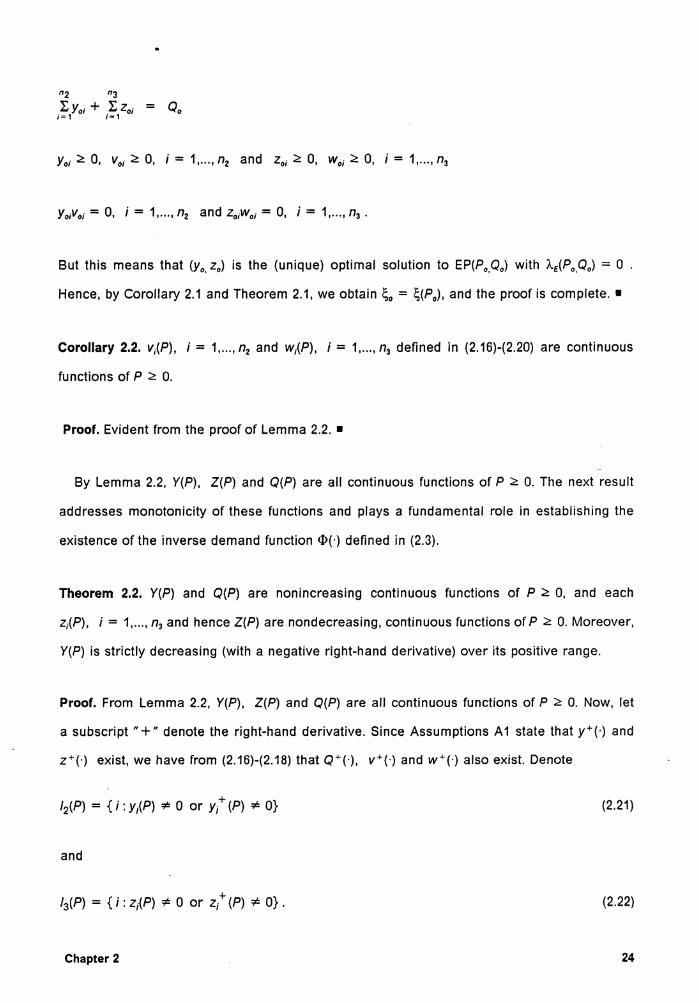
From the development in Murphy et al. [M3], we can conclude that under assumptions

(A1)-(A4), if a certain price P prevails for the semi-finished product purchased by the firms in

S2 , then this elicits a unique equilibrating response y(P) and z(P) from the firms in S2 and S3,

respectively. In fact, as shown in the sequel, under the foregoing assumptions, y(P) and z(P)

are continuous functions of P ~ 0. In view of this, we will assume the reasonable property that

the right-hand derivatives of y(P) and z(P) with respect to P exist, and include this in the above

set of assumptions, henceforth referred to as Assumptions A1.

Now, since the total output of the firms in S1 and S2 must match, when the price established

for the semi-finished product is P the demand faced by the firms in S1 is Y(P). Hence, as P

varies, it generates a derived demand curve for the firms in S1 according to the price reaction

curve Y(P). Under Assumptions A 1, as shown in the sequel, Y(P) is a nonnegative, continuous

function, strictly decreasing over its positive range, say, [O, P0). Denote Y0 = Y(O) and define

for e = 0

for 0 < 0 < Yo

for e ~ Y0

(2.3)

<1>(0), is the (inverse) derived demand function faced by the upstream producers, for the

semi-finished product. This function will be used to define the overall equilibrium solutions in

the two-stage model.

Chapter 2 17

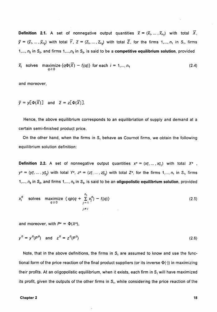
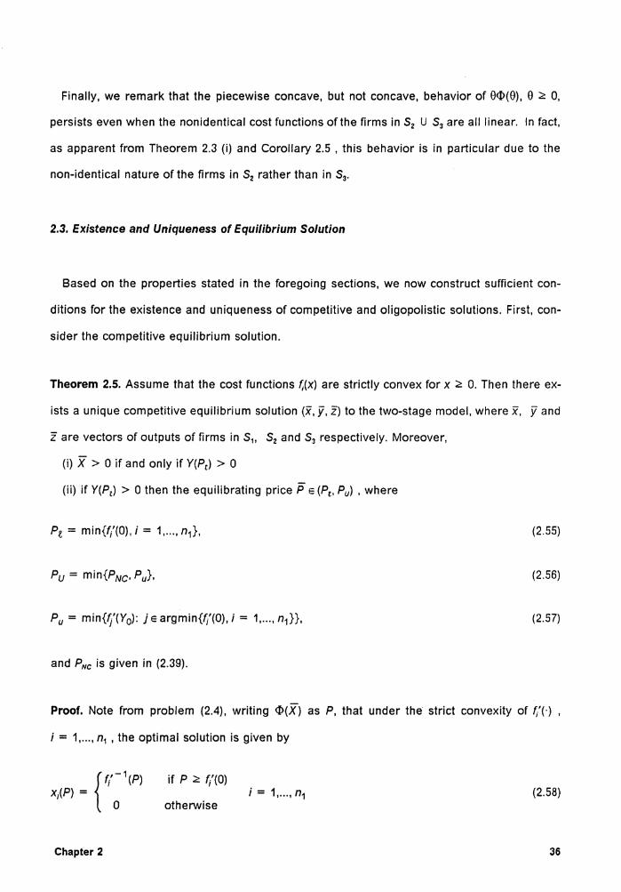
Definition 2.1. A set of nonnegative output quantities x = (x1, .... x,,1) with total X, y = (Y1, ••• , Y,,2) with total Y, z = (z1, ••• , z,,3) with total Z, for the firms 1, ... , n1 in S1, firms

1, ... , n2 in S2, and firms 1, ... ,n3 in S3, is said to be a competitive equilibrium solution, provided

Xi solves maximize {q<l>(X) - f;(q)} for each i = 1, ... , n1 q~O

and moreover,

y = y[ <l>(X)] and z = z[ <l>(X)].

(2.4)

Hence, the above equilibrium corresponds to an equilibriation of supply and demand at a

certain semi-finished produ('.t price.

On the other hand, when the firms in S1 behave as Cournot firms, we obtain the following

equilibrium solution definition:

Definition 2.2. A set of nonnegative output quantities x0 = (xf, ... , x~1 ) with total X0 ,

y0 = (yf, ... , y~2) with total Y0 , z0 = (zf, ... , z~3) with total Z0 , for the firms 1, ... , n1 in S1, firms

1, ... , n2 in S2, and firms 1, ... , n3 in S3, is said to be an oligopolistic equilibrium solution, provided

XO I

n1 solves maximize { qp(q + .l: Xj°) - f;(q)}

q~O j=1

J"" i

and moreover, with P0 = <l>(X0 ),

yo = yo(Po) and zo = zo(Po)

(2.5)

(2.6)

Note, that in the above definitions, the firms in S1 are assumed to know and use the func-

tional form of the price reaction of the final product suppliers (or its inverse <I>(·)) in maximizing

their profits. At an oligopolistic equilibrium, when it exists, each firm in S1 will have maximized

its profit, given the outputs of the other firms in S1, while considering the price reaction of the

Chapter 2 18

firms in S2 U S3 oligopoly. Let X0 be the total output of the firms in S1• Similarly, each firm in

S2 will have maximized its profit by purchasing the semi-finished product at the price

P0 = <l>(X0 ) , given the outputs of the other firms in S2 U S3 , with Y0 = Y(P0 ) = X0 being the

total output of the firms in S2• Finally, each firm in S3 will have maximized its profit, given the

outputs of the other firms in S2 U S3 , with the total production level being Z 0 = Z(P0 ). The

prevailing price for the final product is therefore p(Q0 ) where Q0 = Y0 + Z0 •

2.2.Characterlzation of the Derived Demand Curve

In order to provide facility for establishing the existence of the derived demand curve <I>(·)

and studying its nature, we define below a family of convex programming problems in the

spirit of Murphy et al. [M3]. For a fixed value of P ~ 0 representing the price for the semi-

finished product, and for a fixed value of Q ~ 0 representing the total market supply, consider

the following equilibrating program parameterized by P and Q

EP(P,Q):

n2 n3 n2 n3 n2 n3

maximize{p(Q)( ;~/; + ;~1 z;) + ~ p'(Q) (;~/f + ;~1zf) - 1~p;(Y;) + Py; - ;"f1h;(z;)}

subject to

nz n3 LY;+ L Z; = Q (2.7)

/=1 /=1

Y; ~ O, i = 1, ... , n2 , z1 ~ O, i = 1, ... , n3. (2.8)

The program EP(P,Q) involves the maximization of a strictly concave function over a nonempty

polytope, and consequently a unique optimum exists. Hence, the Karush-Kuhn-Tucker condi-

tions for EP(P,Q), which are both necessary and sufficient for this problem, have a unique

solution. These conditions are rewritten below, where A. is the Lagrange multiplier asso_ciated

Chapter 2 19

with constraint (2.7), and v = (v1, ••• , Yn2) and w = (w1, ••. , Zn3) are the Lagrange multipliers

associated with constraints (2.8).

p(Q) + YtP'(Q) - g/(Yt) - P + Vt - A.= 0, i = 1, ... , n2 (2.9)

p(Q) + Z;P'(Q) - h/(Z;) + Wt - A= 0, i = 1, ... , n3 (2.10)

nz n3 L Yt + L Z; = Q (2.11)

i=1 /=1

Y; ~ 0, v1 ~ 0, i = 1, ... , n2 and Z; ~ 0, w1 ~ 0, i = _ 1, ... , n3 (2.12)

y1v1 = 0, i = 1, ... , n2 and z1w1 = 0, i = 1, ... , n3. (2.13)

Now, given (P,Q) ~ 0, denote by YE(P,Q) and zE(P,Q) the unique optimal solution to EP(P,Q),

and let A.E(P,Q) be the corresponding Lagrange multiplier associated with constraint (2. 7). (In

case Q = 0, whence alternative optimal values exist for this multiplier, define A.E(P,O) to be the

shadow price of Q, i.e., to be the smallest nonnegative optimal multiplier, which is readily

seen to exist via (2.9)-(2.13)). The following result is in the spirit of the analysis in Murphy et

al. [M3]. and relates to the equilibrating nature of program EP(P,Q).

Theorem 2.1. For a fixed P ~ 0, let y and i: represent some nonnegative output vectors of the • "2 "3

firms in S2 and S3 respectively, and denote Q = LY; + L Z;. Then, the quantities y and i: with ;-1 i=1

total output Q constitute a Nash-Cournot equilibrium for the firms in S2 U S3 (hence yielding

y(P) = y, z(P) = z and Q(P) = Q ) if and only if y and z solve EP(P, Q) and moreover,

Proof. The proof follows by simply comparing the necessary and sufficient Karush-Kuhn-

Tucker conditions for problems (2.1) and (2.2) with the corresp~>nding conditions (2.9)-(2.13) for

EP(P, Q). •

Chapter 2 20

. . Hence, with P :l!: 0 fixed, if Q is adjusted to a value Q such that in the problem EP(P, Q), the

optimal Lagrange multiplier associated with (2. 7) vanishes, then by Theorem 2.1, the resulting

optimal solution y = YE(P, Q) ands i: = zE(P, Q) represents a Nash-Cournot equilibrium for the . S2 U S3 oligopoly. In fact, the following result implies that a unique value of such a Q exists in

the interval [o, (n2 + n3)qu), and may be determined via a bisection search based on the sign

Lemma 2.1. Let P :l!: 0 be given and fixed, and let A.E(P,Q), Q :l!: 0 be as defined above. Then

A.E(P,O) ~ 0 > A.E(P, (n2 + n3)qu) . Moreover, A.E(P,Q) is a continuous, strictly decreasing function

ofQ > O, and

(i) A.E(P,Q) < 0 for Q > 0 if A.E(P,O) = 0,

(ii) A.E(P,Q) is continuous at Q = O if A.E(P,O) > 0.

Proof. By definition, A.E(P,O) :l!: 0. Define Qu = (n2 + n3)qu and consider A.E(P,Qu) . Since at least

one firm must produce at least qu in EP(P,Qu), letting this firm's cost function g;(-) or h;(-) be

denoted by G(-), we obtain from (2.9)-(2.13) that A.E(P,Qu) < p(Qu) - G'(qu), since P ~ 0, G{")

is convex and p'(Qu) < 0 . From (A4) this implies that A.E(P,Qu) < p(Qu) - p(qu) :::;; 0 .

The assertion that for any fixed P :l!: 0, A.E(P,Q) is continuous and strictly decreasing in

Q > 0 follows directly from the development in Murphy et al. [M3]. Hence, let us prove parts

(i) and (ii). For notational convenience, let G;(q) = Pq + g;(q), q ~ O for i = 1, ... , n2 and

G;{q) = h;- n2(q), q :l!: 0 for i = n2 + 1, ... , n2 + n3 be the cost functions for the firms in S2 and

53, respectively. Similarly, let g;(Q) be YE;(P,Q) for i = 1, ... , n2 and zE!i- n 21(P,Q) for

i = n2 + 1, ... , n2 + n3• Let G/(O) = min{G/{O), i = 1, ... , n2 + n3}, and note from (2.9)-(2.13) that

A.E(P,O) = max{p(O) - G'k(O), O} .

If A.E{P,O) = 0 then p(O) - G;'(O) :::;; 0 for all i = 1, ... , n2 + n3 and since for each Q > 0 from

(2.9)-(2.13), A.E(P,Q) = p(Q) + q;(Q)p'(Q) - G';[q;(Q)] for some i e {1, ... , n2 + n3}, where

Q;{Q) > 0, we have using p(Q) < p(O), p'(Q) < O and the convexity of Gk) that A.E(P,Q) < 0.

This proves part (i).

Chapter 2 21

On the other hand, suppose that A.E(P,Q) > 0. If qk(Q) = 0 for any Q > 0, then from

(2.9)-(2.13) and the fact that p'(Q) < 0, and that G;(-) is convex for all i = 1, ... , n2 +n3, we get

that A.E(P,Q) ~ p(Q) - G/(O) ~ p(Q) - g/(O) > p(Q) + q;(Q)p'(Q) - G;'[q;(Q)] for any

i e {1, ... , n2 + n3} with q1(Q) > 0, a contradiction to (2.9), (2.10) and (2.13). Hence, qk(Q) > 0 for

all Q > 0, and so from (2.9), (2.10) and (2.13), we get that

(2.14)

Now, as Q ..... o+, qk(Q) must tend to zero by (2.11) and (2.12). Hence, we get from (2.14) that

A.E(P,Q) approaches p(O) - Gk'(O), which equals A.E(P,O) since A.E(P,O) > 0 This proves part (ii)

and completes the proof. •

. . Hence, given P ~ 0, once such a unique value of Q is determined for which A.E(P, Q) = 0 we

have

Q(P) = Q, y(P) = YE(P,Q(P)), z(P) = Zf(P,Q(P)) (2.15)

Corollary 2.1. For any fixed P ~ 0 there exists a unique set of Nash-Cournot equilibrating

outputs y(P), z(P) with totals Y(P), Z(P), for the firms in S2 and S3 respectively. Moreover,

Q(P) = Y(P) + Z(P) satisfies 0 ~ Q(P) < (n2 + n3)qu .

Proof. Follows directly from Theorem 2.1 and Lemma 2.1. •

Based on the foregoing results, y(P) and z(P) are well defined functions of P ~ 0, and hence

so are Y(P), Z(P) and Q(P). The following result establishes continuity of Q(P), y(P) and

z(P).

Lemma 2.2. Q(P), y(P) and z(P) are all continuous functions of P ~ 0.

Chapter 2 22

Proof. First of all, note from Lemma 2.1 and Theorem 2.1 that given any P ~ 0, Q(P) is given . . . by that unique value of Q for which 'Ae(P, Q) = 0 in EP(P, Q), and as in (2.15), y(P) and z(P) are

accordingly obtained as the unique solutions to EP(P,Q(P)). Hence, from (2.9)-(2.13) and (2.15),

given any P ~ 0, Q(P), y(P) and z(P) satisfy the following system of equations, where

V;(P), i = 1, ... , n2 and W;(P), i = 1, ... , n3 are again unique slacks in (2.9) and (2.10) respectively,

for problem EP(P, Q(P)).

p[Q(P)] + Y;(P)p'[Q(P)] - g/[Y;(P)] - P + V;(P) = 0, i = 1, ... , n2 (2.16)

p[Q(P)] + Z;(P)p'[Q(P)] - h/[z;(P)] + W;(P) = 0, i = 1, ... , n3 (2.17)

n2 n3

L Y;(P) + L Z;(P) = Q(P) (2.18) i=1 i=1

Y;(P) ~ 0, V;(P) ::::: 0, i = 1, ... , n2 and Z;(P) ::::: 0, W;(P) ::::: 0, i = 1, ... , n3 (2.19)

Y;(P)v;(P) = 0, i = 1, ... , n2 and Z;(P)w;(P) = 0, i = 1, ... , n3 (2.20)

For the sake of notation, denote ~(P) = (Q(P), y(P), z(P), v(P), w(P)). Now, consider any

P = P0 ::::: 0, and let {Pn} be any nonnegative sequence convergent to P0 • Accordingly, define

~n = (Q(Pn). y(Pn), z(Pn), v(Pn), w(Pn)), and observe that from Corollary 2.1 and (2.16)-(2.20)

that {Sn} is a bounded sequence, and therefore has a convergent subsequence. Without loss

of generality, assume that {~n} is itself convergent to some limit point ~0 • We will show that

Toward this end, observe that for each n, ~n solves (2.16)-(2.20) with P = Pn. Taking limits

as n-+ oo in this system of equations, and noting that p(·). p'(·), g;'('), i = 1, ... , n2 and

h;'("), i = 1, ... , n3 are continuous functions, we obtain

Chapter 2 23

n2 n3

I: Yoi + I: Zo; = Oo i=1 ;-1

Yoi ::::: o. Vol ::::: o. i = 1, ...• n2 and Zo; ::::: o. woi ::::: o. i = 1, ... , n3

But this means that (Y0 • z0 ) is the (unique) optimal solution to EP(P0 ,Q0 ) with Ae(P0 ,00 ) = 0 .

Hence, by Corollary 2.1 and Theorem 2.1, we obtain ~0 = ~(P0). and the proof is complete. •

Corollary 2.2. v;(P), i = 1, ... , n2 and w1(P), i = 1, ... , n3 defined in (2.16)-(2.20) are continuous

functions of P ::::: 0.

Proof. Evident from the proof of Lemma 2.2. •

By Lemma 2.2, Y(P), Z(P) and Q(P) are all continuous functions of P ::::: 0. The next result

addresses monotonicity of these functions and plays a fundamental role in establishing the

existence of the inverse demand function <I>(') defined in (2.3).

Theorem 2.2. Y(P) and Q(P) are nonincreasing continuous functions of P ::::: 0, and each

Z;(P), i = 1, ... , n3 and hence Z(P) are nondecreasing, continuous functions of P ::?! 0. Moreover,

Y(P) is strictly decreasing (with a negative right-hand derivative) over its positive range.

Proof. From Lemma 2.2, Y(P), Z(P) and Q(P) are all continuous functions of P ::::: 0. Now, let

a subscript"+" denote the right-hand derivative. Since Assumptions A1 state that y+(') and

z+o exist, we have from (2.16)-(2.18) that o+o. v+o and w+o also exist. Denote

/2(P) = { i : Y;(P) ;e 0 or Y;+ (P) ;e O} (2.21)

and

/3(P) = { i : Z;(P) ;i!: 0 or Z;+ (P) ;i!: O} . (2.22)

Chapter 2 24

Note that the continuity of Y;(P), Z;(P), V;(P) and W;(P), P ~ 0, along with (2.20) imply that

v1+ (P) = 0 for all i e /2(P) and w1+ (P) = 0 for all i e /3(P) . (2.23)

Taking right-hand derivatives in (2.16)-(2.18) and (2.20), we obtain,

Q+(P){p'[Q(P)] + Y;(P)p"[Q(P)]} + y/{p'[Q(P)] - g/'[y;(P)]} = 1 - v/(P)

(2.24)

Q+(P){p'[Q(P)] + Z;(P)p"[Q(P)]} + z/{p'[Q(P)] - h;"[Z;(P)]} = - w/(P)

(2.25)

L Y1+ (P) + L Z1+ (P) = Q + (P) (2.26) le !2(P) le /3(P)

(2.27)

+ + Z1 (P)w1(P) + Z1(P)w1 (P) = 0 for i = 1, ... , n3. (2.28)

For notational convenience, define

a 1(P) = p'[Q(P)] + Y;(P)p"[Q(P)] for i e 12(P). (2.29)

P1(P) = 1 / {p'[Q(P)] - g{'[y1(P)]} for i e /2(P), (2.30)

and similarly, let

y1(P) = p'[Q(P)] + z1(P)p"[Q(P)] for i e /3(P) (2.31)

o1(P) = 1 / {p'[Q(P)] - h;"[z1(P)]} for i e /3(P). (2.32)

We will show that by Assumptions A1,

Chapter 2 25

ai(P) ~ 0 and ~;(P) < 0, with a;(P) < 0 if Yi(P) < Q(P) for i e /2(P) (2.33)

Y;(P) ~ O and o;(P) < 0, with Y;(P) < O if zi(P) < Q(P) for i e /3(P). (2.34)

First, consider a;(P), i e/2(P). If p"[Q(P)] ~ 0 then a;(P) < 0. On the other hand, if

p"[Q(P)] > 0, then a;(P) ~ p'[Q(P)] + Q(P)p"[Q(P)] ~ 0 by (A2). Moreover, a;(P) < 0 if

y;(P) < Q(P) . The sign of ~;(P) follows directly from Assumptions A1. Similarly, (2.34) holds.

Now, using (2.23) along with (2.24) and (2.25), and the notation (2.29)-(2.32), we get

(2.35)

z;+ (P) = - Y;(P)oi(P)Q + (P) for i e /3(P). (2.36)

Summarizing (2.35) and (2.36) and using (2.26), we get

L ~i(P) Q + (P) = _____ ie_l_2(P_) _____ _

1 + L a;(P)~;(P) + L Y;(P)o;(P) (2.37)

ie /2(P) ie /3(P)

Now, from (2.33) and (2.34), we get that Q+(P) ~ 0, with Q+(P) < 0 if /2(P) :¢: ([). Hence, (2.36)

implies that z/ :::: 0 for all i e /3(P), which means that z+(P) :::: 0. Further, from (2.26),

y+(P) = Q+(P) - z+(P) implies that y+(P) ~ 0, with y+(P) < 0 whenever /2(P) * ([), i.e., by

(2.21), whenever Y(P) > 0. This completes the proof. •

Corollary 2.3. The inverse demand function <1>(0) defined in (2.3) exists and is continuous and

strictly decreasing on 0 ~ e ~ Y0, where Y0 = Y(O).

Proof. From Theorem 2.2, Y(P) is a continuous and nonincreasing function of P :::: 0, being

strictly decreasing over its positive range. Hence, for the proof it is sufficient to demonstrate

that there exists price P0 such that Y(P) > 0 for 0 ~ P < P0 and Y(P) = 0 for all P :::: P0• Let

Chapter 2 26

ZNc = (ZNc1, ... , ZNcn3) denote the unique Nash-Cournot equilibrium solution for the firms in S3,

given that S2 = ©. That is, for each i = 1, ... , n3

n3 zNci solves maximize { qp(q + L zNcj) - hi(q)}

q;::Q j=1 (2.38)

j*i

n3 Furthermore, denoting ZNc = I.zNci we obtain, from (2.16) and (2.21), that Y(P) = 0 if and only

i=1

if p(ZNc) - g/(O) - P :::: 0 for i = 1, ... , n2• Define

PNC= max{O, p(ZNd - min{g/(O), i = 1, ... , n2}}. (2.39)

and note that if PNc = 0 then Y(P) = 0 for all P :::::: 0, and if PNc > 0 then Y(P) > O for

0 :::: P < PNc• and Y(P) = 0 for P :::::: PNc· Letting P0 = PNc competes the proof. •

Corollary 2.4. Suppose that g;(-), i = 1, .. ., n2 are identical. If z(O) > 0 then <I>(·) is continuously

differentiable over its positive range.

Proof. Let g;(-) = g(·), i = 1,. .. , n2• First, we will show that for identical firms in S2, whenever

Y(P) > 0 for any P :::::: 0, we have that /2(P) = {1, ... , n2} and that each of Y;(P), i = 1, ... , n2, are

identical. On the contrary, if for any P :::::: 0, we have yk(P) > y,(P) for some k, f, E {1, ... , n2}, then

from (2.16), (2.19) and (2.20) we get that p[Q(P)] + Yk(P)p'[Q(P)] - g'[yk(P)] - P = 0

~ p[Q(P)] + y,(P)p'[Q(P)] - g'[yc(P)] - P. Hence, using p' < 0 and the convexity of g(-),

this means that 0 > p'[Q(P)] [yk(P) - y,(P)]:::::: g'[yk(P)] - g'[y,(P)] :::: 0, a contradiction.

Therefore, Y;(P) are identical and so are y/(P), and /2(P) = {1, ... , n2} for all P :::: 0 such that

Y(P) > 0.

Now, suppressing the index i, we get from (2.35) that

(2.40)

Further, observe that if z(O) > 0 so that /3(0) = {1, ... , n3}, then we also have /3{P) = {1,. . ., n3}

for all P :::::: 0, since by Theorem 2.2, Z;(P) are continuous and nondecreasing in P :::::: 0 . Con-

Chapter 2 27

sequently, from (2.29)-(2.32) and (2.37), the terms on the right-hand side in (2.40) are all con-

tinuous functions, and so Y(P) and hence <I>(') are continuously differentiable over their

positive ranges. This completes the proof. •

Now we can proceed to characterize the revenue function e<I>(e), for 0 ~ e ~ Y0• (Note that

<I>(e) = 0 for e ~ Y0 .) Our interest in this curve obviously stems from the role it plays in the

optimization problem (2.5) for the upstream producers in S1, being the Cournot firms. In par-

ticular, we would like this revenue curve to be concave so that these problems are linearly

constrained convex programs. In such a case, the existence of a solution to the (simultane-

ous) Karush-Kuhn-Tucker system for (2.5) would imply the existence of an oligopolistic equi-

librium, and one would need to find a solution to this system in order to compute the

equilibrium solution. The next result gives some additional assumptions under which this de-

sirable property of a concave revenue function follows. These assumptions employ a partic-

ular decreasing, concave demand function with a decreasing price elasticity, and require that

the firms in S2 be identical, while nonidentical firms in S3 may be permissible in some cases.

The case of nonidentical firms in S2 is addressed subsequently.

Theorem 2.3. Let p(Q) = a - bQk, where a > 0, b > 0, k ~ 1. Assume that g/('), i = 1,. . ., n2

are identical and convex, and that h;'(·), i = 1, .. ., n3 are identical and concave. Then the func-

tion <I>(e), given by (2.3), is concave in e, 0 ~ e ~ Y0• Moreover, this property of <I>(e) holds

under the alternative modifications of the above assumptions:

(i) k = 1 or 2, and h/(') are concave, i = 1,. . ., n3 (not necessarily identical)

(ii) p(Q) = a - bQ2 - cQ, a > 0, b > 0, c > 0 . and h;(-) are linear (and identical) for

i = 1,. . ., n3•

Proof. Note from (2.3), Theorem 2.2 and Corollary 2.3, that it is sufficient to show that Y(P) is

concave over its positive range. Namely, we need to show that

Y + (P + Ll) ~ Y + (P) for all P ~ 0, Ll > 0 such that Y + (P + Ll) > 0. (2.41)

Chapter 2 28

Let g(·) and h(·) denote the cost functions for the firms in S2 and in S3, respectively. By the

arguments used in the proof of Corollary 2.4, we can conclude that for any P ~ 0, Y;(P) are

identical and so are Z;(P). Hence, from (2.40), eliminating subscripts and suppressing all

function arguments for notational ease, we get by using (2.37), along with (2.29)-(2.32), that

- nz[h" - p' - N3(p' + zp")] y+ = ---------------------

(p' - h")[(p' - g") + n2(p' + yp")] + N3(p' + zp")(p' - g")

where N3 = I /3(P) I. For p(Q) = a - bQk, k ~ 1, this reduces to, upon some simplification,

y+ = - n2(h" + A) (2.42) (bkQk- 1)2(n2 + N3 + k) +Ag"+ bkQk- 2h"[(n2 +1)Q + n2(k - 1)y] + h"g"

where A = bkQk- 2[(N3 + 1)Q + N3(k - 1)z]. (When k = 1 , the terms involving p" above are

automatically zero.) Similarly, when Y(P + .1.) > 0, we have y+(P + .1.) = Yt , say, given by

(2.42) with h", A, Q, g", y, z and N3 replaced by h0", A0 , Q0 , g0", y0 , z0 and N30 respectively,

where the subscript .1 denotes the evaluation of all functions at P + .1. Noting that

Y(P + .1.) > 0 implies Y(P) > Y(P + .1.) > 0 by Theorem 2.2, and that the denominator in (2.42)

is positive, in order to show (2.41), we need to show that the numerator, say, D , of the differ-

ence Yt - y+ is nonpositive, where,

~ = (A + h"){ b2k2Qi!k- 11(n2 + N30 + k) + Aogo"

+ h0"[(n2 + 1)bkQ~- 1 + n2bk(k - 1)y0Q~- 2 + g0"J} - (Ao + ho") [ b2k2QZ!k-1l(n2 + N3 + k) + Ag"

+ h"[(n2 + 1)bkQk-1 + n2bk(k - 1)yQk-z + g"J}.

+ (A + h")(A0 + h/){g0 " - g")

+ bkh"h0"[(n2 + 1)(Q~- 1 - Qk-1) + (k - 1)(Y0Q~-2 - YQk-2)]

Chapter 2 29

+ bzk2[h6HQk-1(n2 + N3 + k) + h"Q~-1(n2 + N36 + k)](Q~-1 - Qk-1)

+ nzb2k2(QQ6)k-1(N3h6n - N36h")

+ (k - 1)b2k2(QQ6)k- 2[h6"(N3YY6 + n2ZZ6) - h"(N36YY6 + n2ZZ6)]

+ (k - 1)b2k2(QQ6)k-z[(n2 + N3 + k - 1)ZY6h6" - (n2 + N36 + k - 1)Z6Yh"]

+ (k - 1)b2k2(QQ6)k-Z(h6 H + h")(ZY6 - YZ6).

Now, from Theorem 2.2., note that y6 < y, z6 ~ z, Q6 < Q, and N36 ~ N3. Moreover, since

g'(') is convex, we have g6 " s: g" and since h'(') is concave, we have h6" s: h". Using these

inequalities, it can be verified that the first term [ ·] is negative, whereas the other terms in

[·] above are all nonpositive. Hence, D < 0. This proves the main part of the theorem, actually

demonstrating that <1>(9), O < e s: Y0 is strictly concave in this case.

To prove modification (i) of Theorem 2.3, we obtain in lieu of (2.42) under the stated condi-

tions when k = 1 that

y+ = - n2(1 + A) where A = :-E b (b + g")(1 + A) + n2b ' ie 13(P) b + h";

(2.43)

Hence, to demonstrate (2.41), we need to show as before that the numerator D of the differ-

ence Yt - y+ is nonpositive, where from (2.43)

Note that g." :s: gn. Further, h/' ~ h16" and so b s: b . Since /3(P) /3(P + .1), L> (b + h/') (b + hj6H)

this therefore implies that A :s: A6 , and hence, D s: 0 above.

Likewise, when k = 2 in part (i) of Theorem 2.3, we obtain in lieu of (2.42) that

y + = - n2( 1 + A) 2n2bQ + (2bQ + g")(1 + A) + 2n2by

(2.44)

where

Chapter 2 30

2b(Q + z,) A= L

ie /3(P) 2bQ + h(

Again, to demonstrate (2.41), we need to show that D :s: 0, where from (2.44)

D = 2n2b[(1 + A)Q6 - (1 + A6)Q] + 2b(1 + A)(1 + A6)(Q6 - Q)

+ (1 + A)(1 + A6)(g6 " - g") + 2bnz(y6 (1 + A) - y(1 + A6)]

Using y6 < y, g6 " :s: g", and Q6 < Q, this gives

Now, observe from (2.45) that

1 ~ z. A = 2b(BQ + C), where B = L and C = ~ ' ie l3(Pl 2bQ + h;" ' ie /3(P) 2bQ + h;"

With this notation, (2.46) may be rewritten as

D 4n2b2 :s: QQ&(B - B&) + (CQ& - QC&) + (y&C - yC&) + (BQy& - B&Qlly).

'

(2.45)

(2.46)

Since Q > Q6 ~ 0, y > y 6 ~ 0, h/' ~ h6 " ~ 0, O :s: Z; :s: Z;6 and /3(P)'!i /3{P + Ll), we get

0 :S: B :S: 8 6 and 0 :s: C :s: C6 • Furthermore, Qy6 - O&Y = y6 (nzY + Z) - y(nzY6 + Z6 ) :s: 0.

Consequently, each term in brackets above is nonpositive, giving D :s: 0. This proves part (i).

The proof of part (ii) requires similar manipulations, and hence is omitted. •

There is one additional situation under which we would like to characterize the revenue

function associated with the derived demand function. This situation is interesting in that it

assumes non-identical firms in both S2 and S3, and hence permits one to empirically study any

differential effects on firms profits due to mergers or integrations. Note that Theorem 2.3 (i)

admits non-identical firms in S3, but requires the firms in S2 to be identical. However, in the

following case, the revenue function turns out to be only piecewise concave (i.e., composed

Chapter 2 31

of a finite number of concave pieces), and one has to deal with nonconvex problems in (2.5).

Nonetheless, as shown in the sequel, this situation is probably one of the most amenable

cases of this type.

Theorem 2.4. Let p(Q) = a - bQ, where a > 0, b > 0. Assume that g/('), i = 1, ... , n2 are con-

vex functions, while h/('), i = 1, ... , n3 are concave. Then

(i) Y;(P), i = 1, ... , n2 are all continuous nonincreasing functions of P :<: 0, strictly decreasing

over their positive ranges

(ii) <I>(·) is continuous, strictly decreasing and piecewise concave over its positive range.

The following two lemmas are useful in establishing Theorem 2.4.

Lemma 2.3. For any P :<: 0 such that /2(P) :¢: <D, the set /3(P) defined in (2.21) is alternatively

given by

/3(P) = {i: W;(P) = O} (2.47)

Proof. First of all note that when /2(P) :¢: <D, (2.22) may be rewritten as

/3(P) = {i: Z;+ (P) > O} (2.48)

since from (2.33) and (2.34), all the quantities in (2.29)-(2.32) are negative in this case. To show

that (2.48) is identical to (2.47), suppose that z/(P) > 0. If Z;(P) > 0, then W;(P) = 0 from (2.20),

and if Z;(P) = 0, then again W;(P) = O from (2.28). Conversely, suppose that z/(P) = 0. Then

we must have Z;(P) = 0 and therefore from (2.25), we have w/(P) = - Q+(P)p'[Q(P)] which

is negative, since /2(P) :¢: <D • This implies that W;(P) must be positive, and hence the proof is

complete.•

Observe by the above result that for any P such that /2(P) :¢: <D ,

i3(P) = {i: z/ (P) = ~} = {i: w1+ (P) < O} = {i: w1(P) > O} (2.49)

Chapter 2 32

. Lemma 2.4. Suppose that p(Q) is a convex function. Then for any fixed P ~ 0 such that . / 2(P) :¢: (/), there exists a ~ > 0 such that

A A A

(2.50)

for all Pe [P, P + ~ ).

Proof. Let us first show that by the convexity of PO , the set /2(P), for any P such that

/2(P) * (/), may be equivalently rewritten as

/2(P) = {i: y/ (P) < O} = {i: Yi(P) > O} (2.51)

Note that it is sufficient to show that for any i e /2(P) , we must have y/ (P) < 0, i.e., by (2.35)

to show that 1 - a1(P)Q+(P) > 0 for any i e /2(P). Using (2.37) , this amounts to demonstrating

that

Since the last term is nonnegative ( actually positive if /3(P) :¢: (/)), we need to show , using

(2.29) on the remaining terms, say, R1, that R1 > 0 for i e /2(P), where

R; = 1 + p"[Q(P)] :E Yj(P)Pj(P) - p"[Q(P)]Y;(P) :E Pj(P). jE i2(P) je i2(P)

(2.52)

Note from (2.30) that pi(P) ~ 1 . Using this in the second term in (2.52) along with the p'[Q(P)]

convexity of PO and the identity Y(P) = :I: yi(P) , we obtain, jel2(P)

R; ~ p'[Q(P)] + p"[Q(P)]Y(P) - p"[Q(P)]y;(P) :E P(P). p'[Q(P)] jet2(P) 1

By the convexity of PO and from Assumptions A1 and (2.33), observe that R1 ~ 0, and so

y/(P) :s: 0. If p"[Q(P)] = 0, then R1 = 1 > 0. Hence, suppose that p"[Q(P)] > 0, since PO is

assumed convex. In this case, if y1(P) > 0, then the second signed term is positive by (2.33),

Chapter 2 33

and since the first term is nonnegative under Assumptions A1, we again have R1 > 0. Finally,

suppose p"[Q(P)] > 0 and y1(P) = 0. Since y/(P) s: 0, and since i e /2(P), we must have

y/(P) < 0, and therefore (2.51) holds.

Now, from (2.51) and (2.49), and using the continuity of y1(') and wi(-) through Lemma 2.2

(along with (2.16) and (2.17)), and using the fact that /3(P) = {1, ... , n3} - fa(P), we obtain (2.50)

for some .1 > 0, and the proof is complete. •

Proof of Theorem 2.4. By Lemma 2.2 y1(P) are all continuous functions, and by (2.51) of Lemma

2.4, since p(Q) is convex, they are also strictly decreasing over their positive ranges. This

proves part (i). For the proof of part (ii) we will show that Y(P) is piecewise concave on

Pe [O, P0]. Observe that for any P ::: 0 and .1 > 0, /2(P)2 /2(P + A) and /3(P)~ i3(P + A), since

y1(P) are nonincreasing, and z1(P), by (2.48) of Lemma 2.3, are nondecreasing in P ::: 0. This,

along with Lemma 2.4 implies that the interval [O, P0) is a sum of a finite number (at most

n2 + n3) of adjacent intervals, say [Pk, Pk+ 1) such that

(2.53)

We will show that in any such interval, y+(P) is nonincreasing in P . Toward this end, consider

any Pe [Pk, Pk+,) and any A > O such that P + A e [Pk, Pk+ 1). Then by equations (2.35), (2.37)

and (2.29)-(2.32), with p(Q) = a - bQ, we obtain

(2.54)

where A = L [b + g/'(y1(P))]- 1 and B = L [b + h/'(z,(P))]- 1 • Readily, the sign of the 1e12(Pk) 1e13(Pk)

difference y+(P + ~) - y+(P) is the same as that of A(1 + b8)(1 + bAA + bBA)

- AA(1 + bBA)(1 + bA + bB), where subscript ~ denotes evaluation at P + A. The last ex-

pression reduces to (1 + bB)(1 + bBA)(A - AA) + b2AAA(B - BA) . But, by the convexity of

g/(') and concavity of h;'(') we have g1A" s: g;" and h1A" ~ ht, hence 0 < A ~ AA and

0 < B ~ BA. Therefore, the considered expression is nonpositive and so y+(P + A) ~ Y+(P)

thus completing the proof of part (ii). •

Chapter 2 34

Corollary 2.5. Under assumptions of Theorem 2.4, suppose that the cost functions

g;{-), i = 1, ... , n2, and h;{-), i = 1, ... , n3 are quadratic or linear. Then

(i) Y;(P), i = 1, ... , n2 and Z;(P), i = 1, .... n3 are all continuous, picewise linear functions of

P ~ 0. Moreover, <1>(0) is continuous, piecewise linear and strictly decreasing over its positive

range.

(ii) If z(O) > O then <1>(0) is a convex and piecewise linear function of e ~ 0.

Proof. Part (i). For any PE [Pk, Pk+ 1) defined by (2.53). the right-hand derivative Q+(P) given

by (2.37) is a constant and so, by (2.35) and (2.36). are Y;+(P) and zt(P). Therefore, Y;(P) and

Z;(P) are all piecewise linear and the proof of part (i) is complete.

Part (ii). Given Theorem 2.4, Corollary 2.3 and the above part (i). it is sufficient to show that

y+(Pk) ~ y+(Pk+ 1L where Pk and Pk+ 1 satisfy equation (2.53). From (2.54) we have

y+(P) _ A 1 + bBk k = k 1 + bAk + bBk '

where Ak, Bk denote the evaluation of expressions A and 8 at P = Pk respectively. Observe

that Bk= Bk+ 1• since z(O) > 0 implies /3(P) = /3(0) = {1, ... , n3} for any P ~ 0. Simultaneously,

completing the proof. •

Note from (2.24) and (2.25) that under assumptions of Corollary 2.6, v;(P), i = 1,. .. , n2 and

W;(P), i = 1,. ... n3 are also continuous, piecewise linear functions of P ~ 0, and moreover, that

w;(P) are nonincreasing in P ~ 0, being strictly decreasing whenever /2(P) :;e: (!) and ii:l3(P).

The proof of Theorem 2.4 actually facilitates the construction of Y(P) function and hence, its

inverse. Namely, as P is increased continuously from zero, the slopes of the various concave

segments of Y(P) via closed form expressions for the individual Y;(P) curves, i = 1,. .. , , n2, and

the breakpoints for the piecewise concave function Y(P) are given by prices at which some

firms in S2 leave the market and/or some firms in S3 enter it.

Chapter 2 35

Finally, we remark that the piecewise concave, but not concave, behavior of 0<1>(0), 0 ~ 0,

persists even when the nonidentical cost functions of the firms in S2 U S3 are all linear. In fact,

as apparent from Theorem 2.3 (i) and Corollary 2.5 , this behavior is in particular due to the

non-identical nature of the firms in S2 rather than in S3•

2.3. Existence and Uniqueness of Equilibrium Solution

Based on the properties stated in the foregoing sections, we now construct sufficient con-

ditions for the existence and uniqueness of competitive and oligopolistic solutions. First, con-

sider the competitive equilibrium solution.

Theorem 2.5. Assume that the cost functions f;(x) are strictly convex for x ~ 0. Then there ex-

ists a unique competitive equilibrium solution (x, y, Z) to the two-stage model, where x, y and

z are vectors of outputs of firms in S1, S2 and S3 respectively. Moreover,

(i) X > 0 if and only if Y(Pc) > 0

(ii) if Y(Pc) > 0 then the equilibrating price Pe (Pi, Pu) , where

Pi = min{f;'(O), i = 1, ... , n1},

Pu = min{'J'(Y0): j e argmin{fi'(O), i = 1, ... , n1}},

and PNc is given in (2.39).

(2.55)

(2.56)

(2.57)

Proof. Note from problem (2.4), writing <l>(X) as P, that under the strict convexity of f;'(") ,

i = 1, ... , n1 , the optimal solution is given by

if P ~ fi'(O) i= 1, ... ,n1 (2.58)

otherwise

Chapter 2 36

n1 Define the aggregate supply curve of the competitive market as X(P) = I: X;(P) . Note that for

;-1

each i, X;(P) is a well defined, continuous and nondecreasing function, being strictly increas-

ing over its positive range. Consequently, so is X(P), and in fact, it is strictly increasing for

P ~ Pc, since fm'- 1(P) , where me argmin{f;'(O), i = 1, ... , n1}, is strictly increasing for P ~ Pc.

Also note that X(P) = 0 for 0 s:: P s:: Pc.

Consider the curve Y(P), and note that P corresponds to a competitrve equilibrium price if

and only if Y(P) = X(P). From Theorem 2.2, Y(P) is a continuous, nonincreasing function of

P ~ 0, being strictly decreasing over its positive range. Hence, the equilibrating output

X = Y = 0 if and only if Y(Pc) = 0. Hence, suppose that Y(Pc) > 0 and recall that X(Pc) = 0.

Then readily, P s:: PNc• since from the proof of Corollary 2.3, Y(P) = 0 for P ~ PNc· Further, from

(2.57) let Pu = t;,'(Y0). Then we have X(Pu) ~ xk(Pu) = t;,'- 1(Pu) = Y(O) :<: Y(Pc). Consequently,

· a unique point of intersection of the curves X(P) and Y(P) exists, and occurs in the interval

(Pc, Pu). This completes the proof. •

Theorem 2.6. Suppose that the assumptions of Theorem 2.3 hold. Then there exists an

oligopolistic equilibrium solution (x0 , y0 , z0 ) to the two-stage model. Moreover,

(i) for any equilibrium solution, the total supply X0 of the firms in S1 is the same, and y0 , z0

are unique,

(ii) if <1>(9) is differentiable at X0 then (x0 , y 0 , z0 ) is unique ,

(iii) X0 > 0 if and only if Y(Pc) > 0, where Pc is defined in (2.55),

(iv) if there exists a competitive equilibrium solution, with a total output of X for the firms in

S1, then X0 s:: X.

Proof, Under the assumptions of Theorem 2.3, <1>(9) is a continuous, strictly decreasing and

concave function of s, 0 s:: 9 s:: Y0• Further, by Assumptions A1, each function f;(·), i = 1, ... , n1,

is continuous, nondecreasing and convex. Hence, from Szidarovszky and Yakowitz [sa]. an

equilibrium solution x0 exists for (2.5), and moreover, the total equilibrating output for the firms

in S1 is the same for any such solution. Therefore, by Corollary 2.1, an oligopolistic equilibrium

(x0 , y0 , z0 ) exists, and y0 , z0 are unique. If <1>(9) is differentiable at X0 , then, again by the de-

Chapter 2 37

velopment in Szidarovszky and Yakowitz [S8]. the solution to problems (2.5) is unique, so that

(x0 , y0 , z0 ) is unique too. Thus the proof of parts (i) and (ii) is complete.

To prove part (iii), we will show that X0 = 0. if and only if Y(P2) = Cl . First, suppose that

X0 = 0. Then x0 = 0 and from the optimality of x0 to problems (2.5), we necessarily have

- f;(O) ~ q<l>(q) - f;(q) for any q > 0, i = 1, ... , n1. Dividing each of these· inequalities by q > O

results in <l>(q) :;;: [f;(q) - f;(O)]/q for any q > 0, which along with the differentiablity off;(") and

the continuity of <I>(·), implies that <l>(O) :;;: f;'(O), i = 1, ... , n1, and hence, that Y(Pi) = 0. Now, for

the reverse implication, suppose that Y(P2) = 0. Then, readily <l>(O) :;;: f;'(O), i = 1, ... , n1, and

further, for any q > 0 we have q<l>(q) :;;: q<l>(O) :;;: qf;'(O), i = 1, ... , n1 • But by the convexity of

f;(·), this gives - f;(O) ~ q<l>(q)- f;(q) for any q > 0, i = 1, ... , n1 • This means that x0 = O is an

optimal solution to problems (2.5). Hence, X0 = 0, and the proof of part (iii) is complete.

Finally, part (iv) follows from the development in Rovinsky, Shoemaker and Todd [R1] and

from Murphy et al. [M3]. and this completes the proof. •

Corollary 2.6. Under assumptions of Theorem 2.6, if Y(P2) > 0 , then P·• e (Pi. PNcL where PNc

is given by (2.39).

Proof. If Y(P2) > 0 then by Theorem 2.6 (iii), Y0 > 0 , which implies that P0 < PNc• since from

the proof of Corollary 2.3, Y(P) = 0 for all P ~ PNc· If P0 :;;: Pi then problems (2.5) yield

X0 = 0 thus contradicting X0 > 0. This completes the proof. •

As suggested by Theorem 2.6, ope may note that if <I>(·) is not diffemntiable at X0 , then the

uniqueness of an oligopolistic equilibrium cannot be claimed, even if the revenue function

9<1>(9) is strictly concave. For example, when <1>(9) = 7 - 9 for O :;;: 9 :;;: 3, and <1>(9) = 10 - 20

for 3 :;;: e :;;: 5 , and there are n1 = 2 firms with identical cost functions f;(x) = 2x, i = 1, 2, one

can verify that x0 = (1.5, 1.5) or (2, 1) or (1, 2) for example, all correspond to oligipolistic equi-

librium solutions. However, as noted in Theorem 2.6 (i), the total output X0 = 3 in each case,

with the semi-finished product price at equilibrium being P0 = <1>(3) = 4. Consequently, from

Corollary 2.1, the equilibrating outputs y 0 and z0 are uniquely determined.

Chapter 2 38

Finally, let us consider the existence of an oligopolistic equilibrium solution when the de-

rived demand function is obtained under the conditions of Theorem 2.4. Because of

nonconcavity of the revenue function, it is difficult to make any global statements regarding

the existence of a simultaneous solution to problems (2.5). However, suppose that we modify

Definition 2.2 to require xr to be a strict local maximizer in (2.5) for each i = 1, ... , n1, and ac-

cordingly, call the solution (x0 , y 0 , z0 ) satisfying this condition along with (2.6) as a local

oligopolistic equilibrium solution. Then we can assert the following:

Theorem 2.7. If n1 = 1, then there exists an oligopolistic equilibrium solution (x0 , y 0 , z0 ). If

n1 :::::: 2 , suppose that in addition, the assumptions of Theorem 2.4 hold. Then there exists a

local oligopolistic equilibrium solution (x0 , y0 , z0 ). In either case, if a competitive equilibrium

(x, y, Z) exists, then O !>: Y0 ·!>: Y.

Proof. In the case of a monopoly (n1 = 1), since the problem (2.5) involves the maximization

of a continuous function essentially over the compact set [O, Y0] under Assumptions A 1, there

clearly exists an oligopolistic equilibrium solution (x0 , y 0 , z0 ). Hence, consider the case of <I>(")

available through Theorem 2.4, and denote its breakpoints by e0 = 0, e1, ... , en_ 1, en = Y0• Ac-

cordingly, let <l>(e), 0 !>: e !>: Y0 be represented as

where <l>t(e) is the fth segment defining <I>(') on [O, Y0].

Now, for each t = 1, ... , n consider the determination of an oligopolistic equilibrium solution

through. (2.5), with <1>(0) replaced by <l>t(e), e :::::: 0. Since <l>t(e), e :::::: 0 is a strictly decreasing,

concave demand curve and the associated revenue function is strictly concave, there exists n1

a unique oligopolistic equilibrium solution (xt, yt, zr), say. If Xt = r. xf lies in the interval i=1

(et-1, 0r), then (xr, yt, zt) is evidently a local oligopolistic equilibrium solution. Hence, suppose

that this condition does not hold for any t = 1, ... , n. Then, there must exist a ·k E {1, ... , n} for

which Xk :::::: ek and Xk+ 1 !>: 0k, since X1 > e0 and xn < en. Now, for any such k, denoting the

Chapter 2 39

slopes of <I>k(') and <I>k+ 10 by sk(') ~ 0 and by sk+ 10 < 0 repectively, define as a function of

9 ::::: 0, for each i = 1, ... , n1, following the approach of Szidarovszky and Yakowitz [S7].

k {x, X; (9) =

0,

such that x ::::: 0 and xsk(9) + <I> k(9) = f;'(x) if it exists (2.59)

if no such x exists,

such that x ::::: 0 and xsk+ 1 (9) + <I> k+ 1(9) = f;'(x) if it exists (2.60)

if no such x exists.

Note that since fi'(x) - xsk(0) is strictly decreasing in x, xt(0), e ::::: 0, is a well defined function.

Moreover, as in Szidarovszky and Yakowitz [S7], this function is readily verified to be con-n1

tinuous and strictly decreasing in e over its positive range. Hence, Xk(0) = L xf(0) is contin-;-1

uous in e ::::: 0, and is strictly decreasing over its positive range. Furthermore, the solution to

Xk(0) = e gives the unique oligopoly equilibrium total output Xk using the demand curve

<I>k{'). Hence, since Xk ::::: ek, we have Xk{0k) ::::: Xk(Xk) = Xk ::::: ek. Similar remarks hold for n1

x1+ 1(0), e ::::: 0, i = 1, .. ., n1 and for Xk+ 1{0) = L x1+ 1(0), with Xk+ 1{0k) ~ ek. Consequently, let ;-1

0 ~ µ0 ~ 1 be such that

and accordingly, define

(2.61)

We will show that xf is a strict local maximizer in (2.5) for each i = 1, ... , n1.

Toward this end, observe from (2.59) and (2.60) that at e = ek, we have, for each

i = 1, ... , n1,

(2.62)

Chapter 2 40

(2.63)

sk(9k) > sk+ 1(0k) so that the objective function in (2.5) is strictly concave in a neighborhood of

x0 • In this case, from (2.62) and (2.63), we have that x7(0k) > 0 , then xr+ 1(0k) < xt(0k), and if

xt(0k) = 0, then <l>k(0k) - f;'(O) :::;;; 0, and so xf+ 1(0k) = 0 as well. Therefore, if xt(0k) > 0, then

from (2.61), xr :::;;; xt(0k) and so from (2.62), we get that

(2.64)

or that the left-hand directional derivative of the objective function in (2.5) at xr is non positive,

which by the strict concavity of the objective function in the neighborhood of x 0 , implies that

the objective value strictly decreases if X; is reduced below xr. Similarly, since xr ~ xr+ 1(0k) for

all i = 1, ... , n1, we get from (2.63) that

(2.65)

or that the right-hand directional derivative of the objective function in (2.5) at xr is non positive.

Therefore, this establishes that x0 defined by (2.61), with the associated y0 and z0 from (2.6)

represents a local oligopolistic equilibrium solution.

cannot arise.

To complete the proof, by denoting P0 = <l>(X 0), I+ = { i: X? > 0} , we get Y(P0 ) = X0 =

1: f;'- 1(P 0 + sx?),where s is the slope of <1>;(0) at X' in case x0 = x; for some i for which iel+

0;_ 1 < X1 < 0;. or otherwise as in the second case above s is suitably chosen from (2.64) and

(2.65) in the interval [sk+ 1(0k), sk(0k)J, noting that <l>k(0k) = <l>k+ 1(9k) = P0 from (2.61). Also, ob-

serve that P0 > f;'(O) for i e I+ and P0 :::;;; f;'(O) for iEI + Therefore, letting X(P), P ~ 0 be as defined

in the proof of Theorem 2.5, we obtain X(P0 ) = L f;'- 1(P0 ). Hence, Y(P0 ) < X(P0 ), and so the iel+

Chapter 2 41

competitive equilibrium occurs at a price lesser than P0 which gives Y > Y0 and this com-

pletes the proof. •

2.4. Summary of Results

In this chapter a two-stage model was analyzed in which the final commodity suppliers are

Cournot firms. For the purpose of characterizing the equilibrating process among the firms in

S2 U S3, a mathematical programming-based approach was employed in the manner intro-

duced by Murphy et al. [M3]. Under general assumptions (A1), we showed that the derived

demand function for the semi-finished product is well behaved, i.e., is continuous and de-

creasing (Theorem 2.2 and Corollary 2.3). Given this derived demand function, we obtained

sufficient conditions for the existence of an equilibrium solution in the model given that the

upstream stage is either perfectly competitive or oligopolistic (Theorems 2.5 and 2.6). For the

latter case, we required that the derived demand function be concave, which in turn imposed

some additional properties of the market demand function and the cost functions for the firms

in S2 U S3• In particular, we required that the downstream producers have identical cost

functions, since otherwise the derived demand function is piecewise concave only, or some-

times even convex ( Theorem 2.4, Corollary 2.5). The issue of computing the equilibrium sol-

utions discussed in this chapter is presented later, in Chapter 4 ( Section 4.1). The next

chapter discusses the two-stage model, with an alternate behavior for the firms In S2 U S3,

namely, a leader-follower type of behavior.

Chapter 2 42

Chapter 3

The Two-Stage Model with a Multiple Leader-Follower Oligopoly

in the Final Product Market

This chapter contains an analysis of the two-stage model, given that the firms in S2 act as

followers while those in S3 act as leaders, in the final commodity market. Assumptions, rele-

vant notation, and definitions are introduced in Section 3.1. Section 3.2 studies the properties

of the aggregate reaction curve of the firms in S2 in response to the input semi-finished prod-

uct price and to the output of the firms in S3• Section 3.3 characterizes the demand curve

perceived by the leader firms in S3• Based on this, Section 3.4 examines the existence and

uniqueness of the multiple leader-follower equilibrium in the final commodity market, charac-

terizing its behavior as a function of the established price for the semi-finished product. The

issues concerning the existence and uniqueness of the overall equilibrium solutions are pre-

sented in Section 3.5. Finally, Section 3.6 contains a summary of results.

3.1.Notat/on, Assumptions and Definitions

For the considered model we assume that the assumptions introduced in Section 2.1 are in

force. For ease in readi.ng we briefly restate them below.

Chapter 3 43

Let p(Q), Q ~ 0 denote the market (inverse) demand function for the final commodity. Fur-

ther let x = (x1, ••• , Xn1) denote the outputs of the n1 firms in S1 with total X, and similarly, let

y = (y1, •.• , Yn2) , with total Y and z = (z1, ••• , Zn3) with total Z denote the otputs of the n2 and

n3 firms in S2 and S3 , respectively. Denote the total industry output by Q = Y + Z. Let the total

cost functions for the firms in S1, S2 and S3 be given by f;(xi), x, ~ 0, for i = 1, ... , n,, gi(Yi),

y1 ~ 0, for i = 1, ... , n2 and h1(z1), zi ::? 0 for i = 1, ... , n3, respectively. We assume throughout that

these functions have the following properties:

(A1) p(Q) is twice differentiable, strictly decreasing, with p'(Q) < 0 for Q > 0,

(A2) p'(Q) + Qp"(Q) s: 0 for all Q ~ 0.

(A3) f;(·), i = 1, ... ,n1, gk), i = 1, ... ,n2, and hk). i = 1, ... ,n3 are nondecreasing, twice

differentiable and convex over the nonnegative real line.

(A4) There exists a quantity qu ~ 0 such that

Recall that as proven by Murphy et al. [M3]. assumptions (A1) and (A2) imply that for each

K ~ 0, Qp(Q + K) is a strictly concave function of Q ~ 0. Also, assumption (A4), along with

(A1) and (A3) simply guarantees the existence of an upper bound of qu on the outputs of the

profit maximizing firms in S2 U S3•

Now, let us present the assumed leader-follower Stackelberg [S6] - Nash [N1] - Cornout

[C1] (SNC) equilibrating process for the firms in S2 U S3, given some prevailing price P ~ 0

for the semi-finished product. For a fixed input price P ~ 0, the effective total cost functions

for the firms in S2 are given by gi(Y;) + Pyi, y1 ~ 0 , for i = 1, ... , n2• Hence, for a given total

output Z ~ 0 of the leader firms in S3, the follower firms in S2 , behaving in a Nash-Cournot

manner, will produce at equilibrium a set of quantities YR(Z,P) = (YR1(Z,P), ... , YRn2(Z,P)), where

for each i = 1, ... , n2, YR;(Z,P) solves the problem:

Chapter 3 44

n2 maximize { qp[q + L YRj(Z,P) + Z] - Pq - g;(q)}

q:zo j=1 (3.1)

j#i

Let us indicate that given an input price P :<?: 0, the quantities YR1(Z,P), ... , YRn2(Z,P) represent a

Nash-Cournot equilibrium solution for the firms in S2, in reaction or response to a given ex-

traneous market supply of Z :<?: 0 units. Consequently, the quantities YR;(Z,P), i = 1, ... , n2, are

referred to as the joint reaction (or response) curves of the follower firms with respect to the "2 .

total supply Z :<?: 0 of the leader firms, and the total reaction YR(Z,P) = L YR;(Z,P) is referred i=1

to as the aggregate reaction curve.

Now, being aware of this aggregate reaction curve of the followers, the leader firms effec-

tively face the following so called perceived demand curve F(Z, P) Z :<?: 0, for any given

p :<?: 0:

F(Z,P) = p[Z + YR(Z,P)]. (3.2)

Hence, at equilibrium, if one exists, the leader firms produce a set of quantities n3

z(P) = (z1(P), ... , Zn3(P)), with a total Z(P) = L Z;(P), where for each i = 1, ... , n3, Z;(P) solves the ;~1

problem:

n3 maximize { qF[q + L zj(P), P] - h;(q)}

q:ZO j=1 (3.3)

j#i

Consequently, we have the following definition.

Definition 3.1 For a fixed input price P :<?: 0, a set of quantities y(P) = (y1(P), ... , Yn2{P)) with total

Y(P), and z(P) = (z1(P), ... , Zn3(P)) with total Z(P), for the follower firms in S2 and the leader firms

in S3, respectively is said to constitute a Stackelberg-Nash-Cournot {SNC) equilibrium solution

in the final product market if Z;(P) solves problem (3.3) for each i = 1, ... , n3 , and

Chapter 3 45

Y;(P) = YR;[Z(P), P]. i = 1, ... , n3, Y(P) = Y R[Z(P), P J. (3.4)

At equilibrium, the total industry output will be denoted by Q(P) = Z(P) + Y(P), for any given

p:::: 0.

In the sequel, we will show that under the foregoing assumptions, YR;(Z,P), Z :::: 0, P ::=: 0 ,

i = 1, ... , n2 are continuous functions, and we will provide some sufficient conditions under

which y(P) and z(P) are also continuous functions of P :::: 0. Whenever such properties hold,

we will make the reasonable assumption (AS) that the right-hand derivatives of these functions

YR;(·,·), y(·) and z(") exist. Notationally, for a function 1j1(s1, s2): R2 -+ R, we will use the symbol

D.~ (IV) to denote the partial right-hand derivative of '1'0 with respect to s;. i = 1, 2, and for a

univariate function ljl{S): R-+ R , we will denote its right-hand derivative by 'V+(s), as in

Chapter 2. Henceforth, assumptions (A1)-(A5) will be referred to as Assumptions A2, and will

be assumed to hold throughout this chapter.

We now begin our analysis by first characterizing continuity, monotonicity, differentiabilty

and convexity properties of the aggregate reaction curve YR(Z,P) Z :::: O under various condi-

tions. This will permit us to characterize certain properties of the perceived demand function

F(Z, P), Z :::: 0, for any P :::: 0 , and further to specify sufficient conditions for the existence and

uniqueness of a SNC equilibrium y(P), z(P) for any P :::: 0. Furthermore, continuity,

monotonicity, differentiablity and convexity properties of Y(P) and Z(P) as functions of P :<! 0

will be investigated. In particular, under some sufficient conditions which guarantee that

Y(P), P :::: 0 is a continuous, nonincreasing function, which is strictly decreasing over its posi-

tive range, say, [O, P0), we define the inverse derived demand function <1>(0) , e :<! 0 in a similar

way as in Chapter 2 (eq. (2.3)):

Chapter 3

for e = 0

for 0 < 0 < Yo

for 0 :::: Y0

(3.5)

46

Based on this definition of the inverse derived demand curve, the overall competitive and

oligopolistic equilibria are defined in the following way.

Definition 3.2. A set of nonnegative output quantities x = (x1, ••. , 'Xn1) with total X ,

y = (Y1, .•• , Yn2) with total Y, z = (z1, ••• , Zn3) with total Z, for the firms 1, ... , n1 in S1, firms

1, ... , n2 in S2, and firms 1, ... ,n3 in S3, is said to be a competitive equilibrium solution, provided

(i) for each i = 1, ... , n1, x, solves

maximize {q<l>(X) - f;(q)} q~O

and

(3.6)

(ii) (Y, Z) = [y(P0 ), z(P0)] if X > 0, where P0 = <l>(X), and (Y, Z) = (0, zNc) if X = 0, where

ZNc denotes a Nash-Cournot equilibrium for the firms in S3 under the demand curve p("). That

is, ZNc = (ZNc1, ••• , ZNcn3) , where for each i = 1, ... , n3, ZNci solves

n3 maximize { qp(q + I ZNc1) - h,(q)}.

q;,O j•1

i"'i

Definition 3.3. A set of nonnegative output quantities x0 = (xf, ... , x~1 ) with total X0 ,

y0 = {Yf, ... , y~2) with total Y0 , z0 = (Zf, ... , z~3) with total Z0 , for the firms 1, ... , n1 in S1, firms

1, ... , n2 in S2, and firms 1, ... , n3 in S3, is said to be an oligopolistic equilibrium solution, provided

(i) for each i = 1, ... , n1, xf solves

n, maximize { q<l>(q + :E xt) - f;(q)}

q~O j=1 (3.7)

j¢i

and the above (ii) in Definition 3.2 with X, (Y, z) replaced by X0 , (y0 , z0 ) respectively holds.

Observe that the above definitions of competitive and oligopolistic equilibrium solutions re-

spectively derive from an assumed market behavior of either perfect competitio.n or a Nash-

Chapter 3 47

Cournot oligopoly on the part of the firms in S1, given the leader-follower Stackelberg-

Nash-Cournot behavior of the firms in S2 and S3 as embodied by Definition 3.1.

3.2.Characterization of the Aggregate Reaction Curve

The purpose of this section is to present some important properties of the aggregate re-

action curve YR(Z,P), Z ~ 0, P ~ 0, which will play a central role in characterizing the per-

ceived demand curve F(Z, P), Z ~ 0, defined in (3.2) for any given P ~ 0, and in characterizing

a SNC equilibrium. First, we demonstrate that YR(Z,P) is a continuous function of Z ~ 0. Next,

using the right-hand derivatives, we study monotonicity and concavity. In particular, we show

that YR(Z,P) is strictly decreasing in Z ~ 0 and in P ~ 0 over its positive range, while

Z + YR(Z,P) is strictly increasing in Z ~ 0. Finally, we provide conditions under which YR(Z,P)

is convex in Z ~ 0 and concave in P ~ O over its positive range. The former property is im-

portant due to problems (3.3), while the latter one is important in establishing concavity of

Y(P). Under Assumptions A2, the reaction curves YR;(Z,P), i = 1, ... , n2 and YR(Z,P) are defined

by the following system obtained via the necessary and sufficient optimality conditions for

problems (3.1):

p[Z + YR(Z,P)] + YR;(Z,P)p'[Z + YR(Z,P)] - g;'[YR;(Z,P)] - p + V;(Z, P) = 0,

i= 1, ... ,n2 (3.8)

nz L YR;(Z,P) = y R(Z,P) (3.9)

i=1

YRi(Z,P) ~ 0, v1(Z, P) ~ 0, i = 1, ... , n2 (3.10)

YR;(Z,P)v1(Z,P) = 0, i = 1, ... , n2 (3.11)

Moreover, for any fixed Z ~ 0 the solution to the above .system is unique (see Sherali, Soyster

and Murphy [SS] and Corollary 2.1), so that the reaction curves YR;(Z,P), i = 1, ... , n2, and

Chapter 3 48

YR(Z,P) are well defined functions for any Z ;;;:: 0. Furthermore, the following continuity and

monotonicity properties hold.

Theorem 3.1. The functions YR1(Z,P), i = 1,. . ., n2, and hence the aggregate function YR(Z,P), are

continuous functions of Z ;;;:: 0 .

Proof. Consider any fixed (Z0 , P0 ) ;;;:: 0 and any nonnegative sequence {(Zk, Pk)} convergent to

(Z0 , P0 ). Define YRk = YR(Zk, Pk) , YRk = YR(Zk• Pk) , and vRk = VR(Zk• Pk) in (3.8)-(3.11). Note that

by Assumptions A2 and equations (3.8)-(3.11), the sequnce {(YRk• vk, YRk)} is bounded, and

therefore has a convergent subsequence. For simplicity, assume that {(yRk• vk, YRk)} is itself

convergent and let (YRo• v0 , YR0 ) denote its limit. We will show that

(YR(Z0 , P0 ), v(Z0 , P0 ), YR(Z0 , P0)) = (YRo• V0, YR0) . Observe that for each k we have p(Zk + YRk) n2

+ YRkP'(Zk + YRk) - g/(YRki) - Pk + Vk1 = 0 for i = 1, .. ., n2, !: YRk1 = YRk and YRki 2 0, Vk1 ~ 0, ;~1

YRk;Vk; = 0 for i = 1,. . ., n2• Noting that the functions p('), p'(') and g/(') are continuous, and

taking limits as k _. 00 , we obtain p(Z0 + YR0) + YR0p'(Z0 + YR0) - g/(YR0 ;) - P0 + V01 = 0 for n2

i = 1,. . ., n2, !: YRoi = YRo and YRoi ~ 0 , v01 ;;;:: 0, YRo;V0 ; = 0 for i = 1,. . ., n2• Since the solution to 1-1

the system (3.8)-(3.11) is unique for any Z;;;:: 0 (see Sherali et al. [SS] and Corollary 2.1), we

Theorem 3.2. The aggregate reaction curve YR(Z,P) is strictly decreasing in Z ~ 0 and in

P :;:: 0 over its positive range. Moreover, Z + YR(Z,P) is strictly increasing in Z :;:: 0. Further-

more. for each i = 1,. .. , n2, the reaction curve YR;(Z,P) is strictly decreasing in Z :;:: 0 over its

positive range, and if p(') is convex, then YR;(Z,P) is also strictly decreasing in P ~ 0 over its

positive range.

Proof. From the development in Sherali et al. [SS] it follows that for any Z ~ 0 the right-hand

(partial) derivative Dz+(YR) of YR(Z,P) with respect to Z satisfies - 1 < Oz+{YR) ~ 0, where the

right inequality is strict whenever YR(Z,P) > 0. Also, Oz+{YR;) ~ 0 for each i = 1, ... , n2• However,

if YR1(Z,P) > 0, then let us show that Dz+(yR1) < 0. Consider some (Z0 , P0 ) ~ 0. If

Chapter 3 49

YR1(Z0 , P0 ) = YR(Z0 , P0 ), then the assertion is immediate from above. Hence, assume that

0 < YR;(Z0 , P0 ) < YR(Z0 , P0 ), and suppose that Df(YR;) = 0. Then, by equations (2.15), (2.16) in

Sherali et al. [SS]. we obtain (using our notation) [ 1 + Df (YR)][p' + YR;(Z0 , P0 )p"] = 0, where

p' and p" are evaluated at Z0 + YR(Z0 , P0 ) • But this means p' + YR;(Z0 , P0 )p" = 0 . If p" :s:: 0 then

a contradiction is evident. Hence, assume that p" > 0. Then we get p' + YR;(Z0 , P0 )p" <

p' + [Z0 + YR(Z0 , P0 )]p" :s:: 0 by assumption (A2), which again results in a contradiction.

Hence, YR;(Z,P) is strictly decreasing in Z ~ 0 over its positive range.

The monotonicity of YR(Z,P), and YR;(Z,P) in P ~ 0 follows readily from Theorem 2.1 and

proof of Lemma 2.4, by noting that for any fixed Z ~ 0, YR;(Z,P), i = 1, ... , n2, is the unique

Nash-Cournot equilibrium solution with an extraneous market supply of Z units. This com-

pletes the proof. •

Before proceeding, let us point out that one can actually derive expressions for the right-

hand partial derivatives Of (YR) and D,t(YR) of YR(Z,P) with respect to Zand P, respectively. In

fact, by differentating equations (3.8)-(3.11) with respect to an increase in Z or P, and noticing

by Theorem 3.1 and (3.8)-(3.11) that for i = 1, ... , n2, v1(·, ·) are continuous and right-

differentiable by Assumptions A2, and moreover, Dz+(v1) = 0 whenever YR1(Z.P) > 0, and

D,t(v1) = O whenever YR1(Z,P) > 0 or D,t(yR1) > 0, we readily obtain

L Ri(Z, P)T;(Z, P) Df (YR) = __ 1_+_ie_J1_(z_,_P_l ------

L R;(Z, P)T;(Z, P) ieJ1(Z,P)

where

Chapter 3

(3.12)

(3.13)

50

J 2(Z, P) = {i: YR;(Z,P) > O or Dft(YR;(Z,P)) > O},

R;(Z, P) = p'[Z + YR(Z,P)] + YR;(Z,P)p"[Z + YR(Z,P)] '

T;(Z, P) = 1/{p'[Z + YR(Z,P)] - g/'[YR;(Z,P)]}, for i = 1,. .. , n2•

Based on this, we can establish the following results related to the differentiability of

YR(·,·), the convexity of YR(·, P) for a given P :::::: 0 and the concavity of YR(Z, ·) for a given

z:::::: 0.

Lemma 3.1. Assume that the firms in S2 are identical, i.e., g;(-) = g(·) for i = 1, ... , n2• Then

YR(Z,P) is differentiable in Z :::::: 0 over its positive range.

Proof. Since 9;(·) = g(·) for i = 1, ... , n2, it follows that for any Z :::::: 0 the unique solution to

(3.8)-(3.11) yields YR;(Z,P) = YR(Z,P)ln2 , i = 1, ... , n2• Therefore, over the positive range of

YR(Z,P), we get J1(Z, P) = J 2(Z, P) = {1, ... , n2} as defined in (3.12) and (3.13). Upon simplifying

and dropping the arguments in equations (3.12) and (3.13) we obtain

(3.14)

(3.15)

where p', and p" are evaluated at Z + YR(Z,P), while g" is evaluated at YR(Z,P)ln2• Notice that

YR(Z,P), p', and g" are all continuous functions, and that p' + YRp" - g" < 0, since it is neg-

ative if p" :s: 0 and if p" > 0, it is strictly less than p' + (Z + YR)p" - g" :s: 0 by Assumptions

(A2) and (A3). Hence, the partial derivatives of YR(·,·) exist and are continuous over its positive

range, being given by (3.14) and (3.15) and this completes the proof. •

Lemma 3.2. Suppose that the industry demand function is given by p(Q) = a - bQk, where

a > 0, b > 0, k :::::: 1. Assume that

Chapter 3 51

(i) k = 1 and g;'(') are concave for i = 1, ... , n2,

or

(ii) k > 1 and g;(-) are linear for i = 1, ... , n2•

Then the aggregate reaction function YR(Z,P) is convex in Z :::: O for any given P :::: 0.

Proof. Part (i) is established in Sherali [S3]. Therefore, consider part (ii). For this purpose we

will demonstrate that for any Z :::: 0 and any Ll > 0, we have Dl,,..(YR) - D/(YR) :::: 0, where the

subscript Ll denotes evaluation at Z + Ll, both here and below. Using the particular form of the

demand and cost functions in equation (3.12), we obtain

where Q = Z + YR(Z,P), and J1 = J 1{Z, P). Therefore, the sign of the- difference

0 2+,,..(YR) - D2+(YR) is the same as that of 8, where

Here, JM = J 1{Z + Ll, P), the functions Q and YRi are evaluated at (Z, P), while Q,,.. and YRil'. are

evaluated at (Z + Ll, P). By Theorem 3.2 we have JMs. J1. Hence, taking the second sum in B

only over JM, we get B :::: (k - 1) I: ( - QyRil'. + Q,,..yR;) . Since, 0,,.. > Q and YR; :::: YR;,,.. by The-iE J1/'.

orem 3.2, this implies that B :::: O and the proof is complete. •

Lemma 3.3. Let the industry demand function be given by p(Q) = a - bQk , where

a > 0, b > 0, k :::: 1. Assume that the marginal cost functions g/(') for i = 1, ... , n2, are identical

and convex. Then for any fixed Z :::: 0, YR(Z,P) is concave in P :::: 0 over its positive range,

being strictly concave over its positive range whenever k > 1.

Proof. It is sufficient to show that the denominator in (3.15) is nondecreasing in P :::: 0, being

strictly increasing if k > 1 . By assumption, g" is a nondecreasing function while YR(Z.P) is

Chapter 3 52

strictly decreasing in P ::::: 0 over its positive range. Hence, for any d ::::: 0,

- g"[YR(Z, P + d)/n2] ::::: - g"[YR(Z,P)ln2]. Therefore, let us focus on the terms involving p'

and p". If k = 1 the result is trivial. Fork > 1, letting O = Z + YR(Z,P) and using the function

p(") specified above, we get that (n2 + 1)p' + YRp" = - bkOk- 2[(n2 + 1)0 + (k - 1)YR] ,

where O and YR are strictly decreasing in P ::::: 0. If k ::::: 2 then the lemma is readily true. For

the case of 1 < k < 2 note that (n2 + 1)0 + (k - 1)YR = (n2 + k)Q - (k - 1)Z. Thus, alterna-

tively, (n2 + 1)p' + YRp" = - (n2 + k)bkOk- 1 + bk(k - 1)0k- 2Z which is again strictly in-

creasing in P ::::: 0, and this completes the proof. •

We remark here that the role played in Lemma 3.1 by the assumption of identical firms in S2

is crucial in avoiding kinks in the aggregate reaction curve which may appear when some, but

not all, of the firms in S2 drop off from production or begin producing under variations in the

parameters Z and P, as governed by Theorem 3.2. This assumption is also necessary in

Lemma 3.3, without which one may only have concavity between the consecutive kink points

in the aggreate reaction curve. Furthermore, the requirement that the demand function p(")

or the cost functions g;(-) , i = 1, ... , n2 be linear as in Lemma 3.2 plays an important role in

establishing the convexity of YR(·, P), given P ::::: 0. For example, if n2 = 1, g(y) = 2.5y2 and

p(O) = 20 - 0.250 2, then for P = 1, problem (3.1) yields 1.5YR(Z, 1) = - (Z + 5)

+ Jo.2sz2 + 10Z + 82, for Z ;;:;: O. One can easily verify that YR(Z, 1) is in fact concave, and

not convex, in Z ::::: 0. Finally, we remark that the particular polynomial form of the demand

function p(Q) = a - bOk , a > 0, b > 0, k ::::: 1, is a direct generalization of a linear demand

curve, and it is strictly decreasing, concave, and has a decreasing price elasticity. Moreover,

it satisfies Assumptions A2. We will be employing this form of the demand function frequently

in our analysis.

Chapter 3 53

3.3. Characterization of the Perceived Demand Function

Recall that the demand function F(Z, P), Z :<::: 0, perceived by by the firms in 53, for any fixed

P :<::: 0, is given by F(Z, P) = p[Z + YR(Z,P)] , Z :<::: 0, as in equation (3.2). Hence, observe that

from Theorem 3.2, as Z :<::: 0, increases for any fixed P :<::: 0 , the function YR(Z,P) decreases,

and if YR(Z,P) gets driven to zero for some Z :<::: 0, the function F(Z, P) will then coincide with

the demand function p(Z) for further increasing values of Z. We are therefore interested in

such a critical value of Z, if it exists. Hence, for any fixed P ::.::: 0 , define

{min{Z :<::: 0: YR(Z,P) = O} if YR(Z,P) = 0 for some Z :<::: 0

Z0(P) = oo otherwise

(3.16)

The following result characterizes Z0(P) and provides an analytical expression for this treshold

value of Z, when it exists.

Lemma 3.4. Let C0 = {P :<::: 0: YR(Z,P) = 0 for some Z :<::: O}. Then C0 is a nonempty connected

set. In particular, if p(Q) = 0 for some finite Q :<::: 0 , then C0 = {P: P :<::: O}. Moreover, Z0(P) is

a continuous and nonincreasing function of P on C0, being strictly decreasing over its positive

range, and for Pe C0 is in fact given by

{p - 1 [P + g' min(O)] if P S: p(O) - g' min(O)

Z0(P) = 0 otherwise

where g' min(O) = minimum{g/(O), i e i = 1, ... , n2}.

Proof. Notice from (3.8)-(3.11) that

YR(Z,P) = 0 if and only if p(Z) S: g'min(O) + P,

(3.17)

(3.18)

where g' min(O) is defined in the lemma. Thus C0 '* (/) as certainly p(O) e C0, and C0 is connected

since P0 e C0 implies Pe C0 for all P :<::: P0 • Furthermore, if p(Q0 ) = 0 for some Q0 < oo, then

Chapter 3 54

0 e C0 because g' min(O) ~ 0 implies that YR(Q0 , 0) = 0, and so C0 = {P: P ~ O}, i.e., a half-line,

in this case. Finally, for any Pe C0, since p(') is strictly decreasing, Z0(P) is readily given by

(3.17) from (3.16) and (3.18). Hence, from (3.17), Z0(P) is continuous on C0, being strictly de-

creasing over its positive range, and the proof is complete. •

Based on this characterization, we obtain the following result relating to the continuity,

monotonicity and differentiability of the perceived demand function.

Theorem 3.3. Let P ~ 0 be fixed. Then the perceived demand function F(Z, P), Z ~ 0, is con-

tinuous and strictly decreasing in Z ~ 0. Moreover, if the firms in S2 are identical, then

F(Z, P), Z ~ 0 is differentiable in Z for Z < Z0(P) and is given by p[Z + YR(Z,P)]. and is

differentiable for Z > Z0(P) (in case Z0(P)· < oo) and is then simply given by p(Z).

Proof. From equation (3.2) and Theorem 3.2, it follows that for any fixed P ~ 0, F(Z, P) is con-

tinuous and strictly decreasing in Z ~ 0. If Z0(P) defined in (3.16) is positive, then for

Z < Z0(P), F(Z, P) given by (3.2) is differentiable in Z by Lemma 3.1. Finally, for Z > Z0(P)

(where Z0(P) < OO), since YR(·, P) = 0 in a neighborhood of Z, we have F(Z, P) = p(Z) and this

completes the proof. •

The role played by the identical firms in S2 is to assure that there is at most one point of

nondifferentiability, namely at Z = Z0(P) , for the perceived demand function F(Z, P), Z :::?: 0.

Furthermore, note that in addition to continuity and monotonicity, we also need some condi-

tions which will guarantee the concavity of F(·, P) in order to make assertions about the ex-

istence of 8NC equilibrium solutions, and to facilitate their computation (in the spirit of Murphy

et al. [M3] or 8zidarovszky and Yakowitz [87, 88]). The next result addresses this issue, and

concludes the characterization of F(·, P) , given P ~ 0.

Chapter 3 55

Theorem· 3.4. Let the industry demand function be given by p(Q) = a - bQk, where

a > 0, b > 0, k ~ 1, and suppose that the marginal cost functions g/O are concave for each

i = 1, ... , n2• Then for any fixed P ~ 0, the function F(Z, P) is concave in Z ~ 0.

Proof. If k = 1 then by Lemma 3.2 and equation (3.2), since F(Z, P) is a concave (linear) and

decreasing function of a convex function, it is concave in Z ~ 0. Hence, suppose that k > 1

and note that the reaction function YR(Z,P) need not be convex in Z in this case. We will show

concavity of F(Z, P) in Z ~ 0 by demonstrating that D/(F) is nonincreasing in Z. By (3.2) and

(3.12) we have:

where as before subscript .£1 denotes an evaluation at Z + .£1 • The denominator in this ex-

pression is positive so we need to show that that for any a > O its numerator, denote it by p,

is negative. Toward this end observe that since p(-) is strictly concave and decreasing, and

since J14S J 1 and R;T1 > 0, one obtains p > l: (p'R;4 T;4 - p'4R;T;) . Further, by the concavity ie.J1A

of g'O , and since YRi& :s: YRi• we have g;" :s: g;4 ". Hence, 0 > T;4 > T;, which along with

p'R;4 > 0 gives P > L T;(p'R;4 - p'l:iR;). By the definition of R1 we get p'R14 - p'6 R1 = le.J1A

p'p6"YR;6 - p'f!.P"YR; , which in case of the demand function specified here, gives

YR;& :s: YRi· Hence, fork> 1, p'R16 - p'4 R1 :s: 0, which along with T1 < 0 implies that p > 0, thus

completing the proof. •

Chapter 3 56

3.4. Existence and Characterization of a SNC Equilibrium as a Function of the Semi-Finished

Product Price

The purpose of this section is to examine the existence and properties of the SNC equilib-

rium solution as a function of P ~ 0, as embodied by the functions y{P) = {y;(P), i = 1, ... , n2}

and z(P) = {z;{P), i = 1, ... , n3}, and their respective totals Y{P) and Z(P) via Definition 3.1. In

particular, under concavity and differentiability properties of F(', P), as may be assured by the

results of the foregoing section, and using some other sufficient conditions, we examine the

existence, continuity, differentiability, monotonicity and convexity properties of the functions

YO and Z(") . First, let us address the existence and uniqueness of a SNC equilibium solution.

Theorem 3.5. Let P ~ 0 be fixed, and assume that the derived demand curve F(Z, P) given by

(3.2) is concave in Z ~ 0. Then there exists a SNC equilibrium solution {y{P), z{P)). Moreover, n3

y{P) is unique, while the total Z{P) = :E Z;{P) is unique over the set of SNC equilibrium sol-i= 1 .

utions.

Proof. By Theorems 3.1 and 3.2, for a fixed P ~ 0, the demand function F(Z, P), Z ~ 0 per-

ceived by the firms in S3 is continuous and strictly decreasing. Therefore, if F(Z, P) is concave

in Z ~ 0 then from the development in Szidarovszky and Yakowitz [S8] it follows that for any

fixed P ~ 0 the set of solutions to problems (3.3) is nonempty, and moreover, the total output

Z{P) is the same for any such solution. This further implies that y{P) defined in (3.4) exists and

is unique , and the proof is complete. •

Corollary 3.1. In addition to assumptions of Theorem 3.5, suppose that F(Z, P) is differentiable

in Z at Z = Z(P). Then there exists a unique SNC equilibrium solution {y{P), z{P)).

Proof. Follows from Szidarovszky and Yakowitz [Sa], using the assertion of Theorem 3.5. •

Chapter 3 57

Corollary 3.2. In addition to assumptions of Theorem 3.5, suppose that the firms in S2 are

identical with gk) = g(·) for i = 1, ... , n2, and suppose that Y(P) > 0. Then there exists a unique

SNC equilibrium solution (y(P), z(P)).

Proof. Let P = P0 ~ 0 be fixed such that Y(P0 ) = YR[Z(P0 , P0)] > 0. If Z(P0 ) = 0 then the result

follows from Theorem 3.5. Hence, suppose that Z(P0 ) > 0. By Lemma 3.1, YR(Z, P0 ) is

differentiable in Z at Z = Z(P0 ) = 0 , and hence so is F(Z, P0 ). Using Corollary 3.1, this com-

pletes the proof. •

Observe that Theorem 3.5 asserts that when F(·, P) is concave, the equilibrating quantities

y(P), Y(P) and Z(P) are uniquely determined, and hence y(P), Y(P) and Z(P) are well defined

functions of P ~ 0. The two corollaries to the theorem provide conditions under which z(P) is

also uniquely determined. The next theorem and its corollaries address the behavior of these

quantities as functions of P .

Theorem 3.6. Assume that F(Z, P) is concave in Z ~ 0 for each fixed P ~ 0. Then

y(P) = {y;(P), i = 1, ... , n2} , Y(P), Z(P) and Q(P) = Y(P) + Z(P) are all continuous functions of

p ~ 0.

Proof. First, note by Theorem 3.5 that Z(P), y(P), Y(P) and Q(P) are all well defined functions.

Secondly, if Z(P) is a continuous function then by Theorem 3.1, Y;(P) = yR;[Z(P), P] ,

i = 1, ... , n2 and Y(P) = YR[Z(P), P] , P ~ 0 are also continuous, and hence so is

Q(P) = Z(P) + Y(P). Therefore, it is sufficient to show continuity of Z(P), P ~ 0. Toward this

end, consider a nonnegative sequence {Pk}-+ P0 and let Zk = Z(Pk). The sequence {Zk} being

nonegative and bounded (by Assumption (A4)) has a convergent subsequence. Without loss

of generality assume that {Zk} itself converges, and let Z0 denote its limit. We must show that

Z0 = Z(P0). Now, for each k let zk be a vector of equilibrating outputs for the firms in S3 with n3

total Zk. From Theorem 3.5, although zk is not unique, we have the same total .r zk1 = Zk. Since 1=1 •

Chapter 3 58

n3 {zk} is contained in a compact set, let {zk}K ..,,. z0 over an index set K, and note that .I: Z0 ; = Z0

1=1

. Then, from (3.3), we have from each i = 1, ... , n3 and any q > 0 that

for each k. Taking limits ask..,,. oo, k eK we obtain

for all q ::;:.; 0, i = 1, ... , n3• But this means that at P = P0 , z0 is an equilibrium solution with total

Z0 , which implies that Z(P0 ) = Z0 , and hence the proof is complete. •

Corollary 3.3. Under assumptions of Theorem 3.6, z(P) is a closed point-to-set map.

Proof. Evident from the proof of Theorem 3.6.•

Corollary 3.4. In addition to assumptions of Theorem 3.6, suppose that for a given P0 , F(Z, P)

is differentiable in Z at Z = Z(P) for each P in some neighborhood of P0 • Then z(P) is a con-

tinuous function of P in some neighborhood of P0 •

Proof. Follows from Corollaries 3.1 and 3.3. •

From Theorems 3.5 and 3.6, although the total equilibrating output Z(P) of the firms in S3 is

a continuous function of P ::;:.; 0, the individual equilibrating output vector z(P) constitutes only

a closed point-to-set map in general as in Corollary 3.3, unless some additional conditions

such as the one in Corollary 3.4 hold. The following result addresses the monotonicity and

differentiability of the total equilibrating quantities Y(P), Z(P) and Q(P) as functions of P ::;:.; 0.

These conditions will be useful in establishing the existence and uniqueness of equilibrium

solutions in the two-stage model.

Chapter 3 59

Theorem 3.7. Let the industry demand function be given by p(Q) = a - bQk , where

a > 0, b > 0, k ~ 1, and assume that the firms in S2 are identical, with g;(-) = g(·) for

i = 1, ... , n2 , where g(·) is a quadratic or a linear function. Then for any P ~ 0 such that

Y(P) > 0

(i) z+(P) ~ 0, with z+(P) > 0 if Z(P) > 0

(ii) y+(P) < 0, and Q+(P) < 0.

Proof. First of all, note from Theorems 3.4 and 3.6 that Z(P) , Y(P) and Q(P) are all continuous

functions of P ~ 0. Now, consider some P = P0 such that Y(P0 ) > 0. If Z(P0 ) = 0 then evidently

z+(P0 ) ~ 0. Hence, suppose that Z(P0 ) > 0. By assumption, g;(') = g(·) for i = 1, ... , n2, so that

by Lemma 3.1, YR(Z,P) is differentiable in Zand in P over its positive range. Furthermore, since

Y(P0 ) > 0, where recall that Y(P) = YR[Z(P), P]. we can conclude that F(Z, P) is differentiable

in Z at Z = Z(P) for all P in some neighborhood of P0 , which by Corollary 3.4 implies that

z(P) is a continuous function of P in some neighborhood of P0 • Now, define J3(P) = {i: Z;(P) > 0 or z/(P) > O} and observe that by the necessary and sufficient conditions for

problems (3.3), we get

p[Z(P) + Y(P)] + p'[Z(P) + Y(P)][ 1 + -t-YR(Z(P),P)]z;(P) - h/[z;(P)] = 0 oz (3.19)

and ::E Z;(P) = Z(P) for all P in some neighborhood of P0 • (Note that the optimal Lagrange ieJ3(P)

multiplier associated with nonnegativity constraint in (3.3) is zero for all P e [P0 , P0 + i:]for

some i; > 0, for any i e J3(P0 ).) Let us now take the right-hand derivative of (3.19) with respect

to (an increase in) P and evaluate it at P0 • Noticing that whenever Y(P) > 0, we have

y+(P) = a~ YR[Z(P), P]Z+(P) + a~ YR[Z(P). P] , and using equations (3.14) and (3.15), we

obtain upon some simplification (for the sake of notation the arguments of the functions used

below are omitted):

(3.20)

Chapter 3 60

where

V = (n2 + 1)p' + p"YR,

a-=p'(1+~Y)-h" I az R I'

and where

A, = p'(V - g")2 + (p' - g")[(p")2 - p'p"']z,YR + p'p"z,(V - p' - g") + p"(g")2Z;.

Summing up equations (3.20) for i eJ3(P0 ), we obtain

Z + (P 0)[(V - g")2 + l: ;; la1] = - l: 11; la;. (3.21) ie J3 ie J 3

Observe that a1 < 0 and A1 < 0, and hence, ; 1 < 0 while 111 > 0. Therefore, equation (3.21)

implies that z+(P0 ) > 0, thus completing the proof of part (i).

Now, let us prove part (ii). Recall that y+(Po) = a~ YR[Z(Po), Po]Z+(Po) + a~ YR[Z(Po), po].

Since z+(P0 ) ::::: 0 from above, and since by Theorem 3.2 both the partial derivatives of YR(',·)

are negative, we get y+(P0 ) < 0. Finally, we will show that Q+(P0 ) < 0. By definition, we have

Q+(P0 ) = z+(P0 ) + Y+(P0 ) • If z+(P0 ) = 0 then readily Q+(P0 ) < 0 . Hence, suppose that

z+(P0 ) > 0 Then, by equations (3.14), (3.15) and (3.21), and denoting

W = (V - g")2 + l: ~1 1a;. we obtain Q+(P0 ) = ~YR[(V - g")2 + p'p"(p' - g") l: z1 /a;]/W. 1eJ3 8P 1e13

The term in [·] is positive which along with a~ YR < 0 and w > 0 implies that Q+(Po) < 0 '

thus completing the proof. •

Corollary 3.5. Under assumptions of Theorem 3.7, there exists price P0 ~ O such that

Y(P) > 0 for 0 s: P < P0 and Y(P) = 0 for P ::::: P0•

Chapter 3 61

Proof. If Y0 = 0, then P0 = 0 since from the proof of Theorem 3.7, we obtain Y(P) = 0 for all

P ~ 0. On the other hand, if Y0 > 0, then from (3.4) and (3.16), we necessarily have

0 ~ Z(O) < Z0(0). Moreover, Y(P) > 0 for all P ~ 0 such that Z(P) < Z0(P), and Y(P) = 0 for all

P ~ 0 such that Z(P) ~ Z0(P). But from Lemma 3.4, Z0(P) is continuous in P ~ 0 and strictly

decreasing over its positive range, while Z(P) is continuous in P ~ 0, being nondecreasing

over the positive range of Y(P). Hence, there exists a price P0 > 0 such that Z(P) < Z0(P) for

0 ~ P < P0 and Z(P) ~ Z0(P)for P ~ P0• Therefore, Y(P) > 0 for Pe [O, P0) and Y(P) = 0 for

P ~ P0, and this completes the proof. •

Remark 3.1. From the proof of Theorem 3.7 and Corollary 3.5, it follows that if Y0 = Y(O) > 0,

then Z(P) > 0 for all Pe [O, P0 ] if Z(O) > 0, and if Z(O) = 0 while Z(P0) > 0 , then there exists

a Pz, where 0 < Pz < P0 , such that Z(P) = 0 for all Pe [O, Pz], and Z(P) > 0 for Pe (Pz, P0].

Finally, if Z(P0) = 0, then Z(P) = 0 for all Pe [O, P0].

Corollary 3.6. In addition to the assumptions of Theorem 3.7, suppose that the cost functions

h;(-). i = 1, ... , n3, are.identical, and assume that P0 > 0. If Z(O) = 0 and Z(P0) > 0, let Pz be as

defined above, and otherwise, arbitrarily let Pz = 0. Then Y(P) and Z(P) are differentiable for

Pe (0, Pz) and for Pe (Pz, P0) •

Proof. From Theorem 3.4 and Corollary 3.2 it follows that for all P such that Y(P) > 0, since the

firms in S2 as well as in S3 are identical, Z;(P) is given by Z(P)/n3 for i = 1, ... , n3 via (3.19). But A A A A

this implies that for any Pe (Pz, P0), we have Y(P) > 0 and Z(P) > 0, so that /3(P) = {1, ... , n3},

and from (3.21), (3.14) and (3.15), we can claim that z+(P) exists and is continuous in a

neighborhood of P and so Z(P) is·differentiable at P. Since Y(P) = YR[Z(P), P]. we have from . Lemma 3.1 that Y(P) is also differentiable at P. Hence, Y(P) and Z(P) are both differentiable

on (Pz, P0).

If Pz > 0, then Z(·) is also differentiable on (0, Pz) since Z(P) = 0 for Pe [O, Pz]. Furthermore,

since Y(P) = YR[Z(P), P] and Y(P) > 0 for Pe (0, Pz) as Pz ~ P0, it follows from Lemma 3.1 that

Y(") is also differentiable on (0, Pz) , and this completes the proof. •

Chapter 3 62

The ingredients of Theorem 3.7 are constructed from Lemma 3.1, Theorems 3.3 and 3.4, and

the consequences of these results given in Theorem 3.6 and Corollary 3.4. Actually, in Theo-

rem 3.7, if one assumes that Y(P), Z(P), and Q(P) are all continuous in P ~ 0, and replaces the

particular form of p(Q) by the assumption that p(Q) is concave and that [p"]2 ~ p'(Q)p"'(Q) for

all Q ~ 0, then from the proof of theorem, it can be readily shown that the result continues to

hold. On the other hand, the assumption of identical firms in S2 is crucial for the assertion in

Theorem 3.7. In fact, if one relaxes this assumption, then even with linear demand and cost

functions, and with n3 = 1, the function Z(P) need not be monotone, and the function Y(P) need

not be strictly decreasing over its positive range. For example, when p(Q) = 20 - Q, and

n2 = 2 with g1(y) = g2(y) = By, and n3 = 1 with h(z) = 10z, we obtain from the solution to (3.1)

that

(

2(14 - z - P) /3 for (Z + P) E [O, 8]

YR(Z,P) = (16 - Z - P) 12 for (Z + P) e [8, 16]

0 for (Z + P) e [16, OO)

Using the above reaction function in problems (3.3) we get

1 + p for Pe [0, 3.5]

8-P for p E [3.5, 4]

Z(P) = 2 + 0.5P for p E (4, 28/3]

16 - p for Pe[28/3,11]

5 for p E [11, 00)

which gives

2(13 - 2P)/3 for PE [0, 3.5]

4 for p E (3.5, 4] Y(P) = YR[Z(P),P] =

7 - 3P/4 for PE [4, 28/3]

0 for p E [28/3, 00)

Chapter 3 63

Hence, for Pe [3.5, 4]. Z(P) is strictly decreasing and Y(P) remains constant, while still being

positive.

Corollary 3.7. Under assumptions of Theorem 3.7, suppose that Y0 > 0. Then, the derived de-

mand function <1>(0) is continuous , being strictly decreasing on (0, Y0). If in addition, the firms

in S3 are identical, then <1>(0) is differentiable in this interval, except perhaps at 0 = Y{Pz) .

Proof. Follows directly from (3.5) and Corollaries 3.5 and 3.6. •

Remark 3.2. Characterization of Z(P), P :<?: 0 under the assumptions of Theorem 3.7.

Suppose that P0 > 0. If Z(O) > 0, then Z(P) is continuous and strictly increasing on [O, P0],

and if the firms in S3 are identical, then it is also differentiable on (0, P0) • If Z(O) = 0, then

Z(P) = 0 for Pe [O, Pz] , and Z(P) is strictly increasing in P for Pe (Pz, P0). Furthermore, Z(P)

is also differentiable on (0, Pz), and on {Pz, P0) if the firms in S3 are identical.

Next, as in Definition 3.2, let ZNc = (ZNc1, ... , ZNcn3) denote the Nash-Cournot equilibrium sol-

ution for the firms in S3, given that they face the demand function p(Z) (with the firms in S2 n3

being absent), and let ZNc = ~ zNc; . From Szidarovszky and Yakowitz [sa], zNc is unique. i-1

Furthermore, from Lemma 3.4 and under the assumptions of Theorem 3.7, C0 = {P: P :<?: O}

and so 0 s: Z0(P) < oo in (3.16) for all P :::: 0. Now, observe that minimum{P :::: 0: Z0(P) s: ZNc}

is well defined by Lemma 3.4. Moreover, from (2.39) and (3.17) we have

PNC = minimum {P :;::: 0: Za(P) s: ZNd· (3.22)

Therefore, if ZNc = 0, then for P > PNc• Z0(P) = 0 from (3.16) and (3.22), and since by Theorem

3.3, the perceived demand function coincides with p('), we have Z(PNc) = ZNc = 0. On the other

hand, if ZNc > 0, then for P > PNc• since Z0(P) < ZNc by (3.22) and Lemma 3.4, it follows that

ZNc solves problems (3.3) (uniquely by Theorem 3.3 and Corollary 3.1), because ZNc lies on the

differentiable segment of the concave perceived demand curve F(·, P), which coincides with

p(') by Theorem 3.3. Hence, in either case, by continuity of Z(P), we get Z(P) = ZNc for

P :<?: PNc· By Theorem 3.7, therefore, we must have PNc :::: P0• Summarizing,

Chapter 3 64

Z(P) = ZNc for P ~ PNc• where PNc ~ P0•

Finally, consider Pe [P0, PNcJ. and note that if Z(P) < Z0(P) , then Y(P) is positive by (3.16)

which is a contradiction because P > P0• Furthermore, if Z(P) > Z0(P) , then since Z(P) lies on

the differentiable segment of the perceived demand function F(-, P) which coincides with p(')

by Theorem 3.3, it must be that Z(P) = ZNc• which contradicts P < PNc by (3.22). Therefore,

Z(P) = Z0(P) given by (3.17) for PE [P0, PNc] .

We will now proceed to examine the convexity properties of Z(P) and Y(P) over the positive

range of Y(P). In particular, as in Chapter 2, attention is focused on establishing sufficient

conditions under which <I>(-) is concave over its positive range, i.e., when it coincides with the

inverse of Y(') . This will imply that the optimization problems (3. 7) for the upstream producers

are convex programming problems, and will be useful in establishing the existence and

uniqueness of an overall equilibrium solution. The following results address these convexity

properties.

Lemma 3.5. Suppose that the industry demand function p(') is linear, the firms in S2 are iden-

tical with g;(-) = g(·) for i = 1, ... , n2 , where g(') is quadratic (or linear), and the marginal cost

functions h;'('), i = 1, ... , n3 are concave. Then Z(P) is convex for 0 ~ P ~ P0•

Proof. If P0 = 0, the proof is trivial. Hence, suppose that P0 > 0 and consider some P0 E [O, P0}

so that Y(P0 ) > 0. By the linearity of p(·) we obtain in the proof of Theorem 3.7 that A; are

identical and negative, and so, ~1 are also identical and negative, and 111 are identical and

positive. Therefore, from (3.20), z/(P0 ) has the same sign for all i eJ3(P0 ), which along with

that Y(P0 + Ll) > 0 , and by the concavity of h;'('), h/'(z16) ~ h/'(z1) , where the subscript Ll de-

notes an evaluation at P0 + Ll. From (3.17), 1 + a~ YR is a positive constant, and so

L ( - 1/u16) ~ L ( - 1/u;) > 0 . Hence, from (3.22), since V - g" is a constant, we obtain le J31!. ieJ3

z+(P0 ) ~ z+(P0 + Ll), which means that Z(P) is convex for 0 ~ P < P0, and hence on [O, P0]

by continuity. This completes the proof. •

Chapter 3 65

Theorem 3.8. Let p(Q) = a - bQk, where a > 0, b > 0, k ~ 1. Suppose that g/(-) = g'(-) for

i = 1, ... , n2, and assume that the marginal cost functions h/(·) , for i = 1, ... , n3 are concave.

Then <1>(9) defined by (3.5) is concave in.9, 0 ~ 9 ~ Y0 if one of the following two conditions

holds:

(i) k = 1 and g(·) is quadratic or linear

(ii) k > 1, g(·) is linear, and the firms in S3 are identical with h1(') = h(·) being thrice

differentiable for i = 1, ... , n3•

Moreover, under condition (ii), <1>(9) is strictly concave for O ~ 9 ~ Y0 •

Proof. Below part (i) is. established. The proof of part (ii) is very long and therefore, is releg-

ated to Appendix A. If Y0 = 0 , the result is trivial. Hence, suppose that Y0 > 0. As in the proof

of Theorem 2.3, it is sufficient to show that Y(P) is concave over its positive range. To establish

this we will demonstrate that the right-hand derivative Y+(P) is nonincreasing in P ~ 0 over

the positive range of Y(P), i.e., for Pe [O, P0) ,by Corollary 3.5. By assumption all the firms in

S2 are identical and so YR(Z,P) is differentiable in Z and in P over its positive range, by Lemma

3.1. Therefore,

(3.23)

where the partial derivatives are given by (3.14) and (3.15). From these equations, since g"(')

is a nonnegative constant, while p'(') is a a negative constant, it follows that both the partial

derivatives are negative constants. Furthermore, by the linearity of p('), and the concavity of

h;'(') , i = 1, ... , n3, we obtain from Lemma 3.5 that z+(P) is nondecreasing in Pe [O, P0), and so

from (3.23) Y+(P) is nonincreasing in Pe [O, P0), and this proves case (i). •

3.S. Existence and Uniqueness of Equilibrium Solutions

The purpose of this section is to establish the existence and uniqueness of equilibrium sol-

utions defined in Definitions 3.2 and 3.3, under the assumptions of Theorem 3. 7, which ensure

Chapter 3 66

the existence of <1>(9) defined in (3.5). Before proceeding, one noteworthy comment regarding

Definitions 3.2 and 3.3 in light of Remark 3.2 is that whenever at equilibrium X = 0 or

X0 = 0, so that Y = 0 or Y0 = 0, respectively, the equilibrium price for the semi-finished

product can be taken as any value not smaller that P0• However, noting the behavior of Z(P)

for Pe [P0, PNcJ. since the firms are effectively nonexistent in this case, we may take

P = PNc (P 0 = PNc) or greater so that ZNc is the unique equilibrating output for the firms in

S3• Hence, we have

_ [<l>(X) if x > o P=

PNc otherwise {

<l>(X 0 ) if X0 > 0 pO =

PNc otherwise (3.24)

The following results provide sufficient conditions for the existence and uniqueness of the

overall equilibrium solutions and are the counterparts of Theorems 2.5 and 2.6, established in

the case of the follower-follower oligopoly in the final commodity market.

Theorem 3.9. Suppose that the assumptions of Theorem 3.7 hold, and let the cost functions

f;('), i = 1, ... , n1 for the firms in S1 be strictly convex and increasing over the nonnegative real

line. Then there exists a unique competitive equilibrium solution (x, y, z) to the two-stage

model. Moreover,

(i) X > 0 if and only if Y(Pc) > 0

(ii) if Y(Pe) > 0 then P e (Pc, Pu) where

Pt = min{f;'(O), i = 1, ... , n1} (3.25)

(3.26)

Pu= min{~'(Y0): j e argmin{f;'(O), i = 1, ... , n1}}. (3.27)

Proof. From the proof of Theorem 2.5, it follows that there exists a unique solution x to prob-

lems (3.6), and moreover, (i) and (ii) hold. Thus, since X is unique, (3.24) defines P uniquely

Chapter 3 67

by Corollary 3.7. By Theorems 3.4 and 3.5 it remains to show that z = z(P) is unique. If

X = 0, then y = 0 and z = z(P) is unique (see Szidarovszky and Yakowitz [SB]). On the other

hand, if X > o then Y(P) > o which by Corollary 3.2 implies that (Y, z) is uniquely determined,

and this completes the proof. •

Theorem 3.10. Suppose that the assumptions of Theorem 3.8 hold. Then there exists an

oligopolistic equilibrium solution (x0 , y0 , z0 ) to the two-stage model. Moreover,

(i) for any equilibrium solution, the total supply X0 of the firms in S1 is the same, and y0 , z0

are unique,

(ii) if <1>{0) is differentiable at X0 then {X0 , y0 , z0 ) is unique ,

(iii) X0 > 0 if and only if Y(Pc) > 0, where Pc is defined in (3.25),

(iv) if there exists a competitive equilibrium solution, with a total output of X for the firms in

S1, then X0 ::::: X.

Proof. From Corollary 3.7 and Theorem 3.B, there exists a solution x0 to the problems (3.7) with

a unigue total output value X0 by the results in Szidarovszky and Yakowitz [S8]. Furthermore,

by the same argument as in the end of the proof of Theorem 3.9, it follows that the accompa-

nying equilibrating outputs (y0 , z0 ) are unique since X0 is unique. This establishes the exist-

ence of an oligopolistic equilibrium and also proves part (i). If <1>(0) is differentiable at X0 , then

x0 is unique since <1>(0) satisfies the conditions in Szidarovszky and Yakowitz [SB] by Corollary

3.7 and Theorem 3.8, and so part (ii) follows from (i). Parts (iii) and (iv) follow directly from the

proof of Theorem 2.6. •

Corollary 3.8. Under assumptions of Theorem 3.10, if Y(Pi) > 0 , then P0 E (Pc, PNc), where PNc

is given by (3.22).

Proof. Result follows from Theorem 3.10 and the proof of Corollary 2.6. •

Chapter 3 68

Corollary 3.9 Let the assumptions of Theorem 3.8 hold, and let the firms in S3 be identical with

h;(-) = h(") for i = 1, ... , n3• If (x0 , y0 , z0 ) is an oligopolistic equilibrium with z0 > 0 , then this is

a unique equilibrium solution.

Proof. If X0 = 0, then the assertion is evident from Theorem 3.8. Hence, suppose that X0 > 0,

so that Y0 > 0. Since all the firms in S3 are identical and since Z0 > 0 , Y(P) is differentiable

at P = P0 by Corollary 3.5, and so <1>(9) is differentiable at X0 • Therefore, by Theorem 3.10 (ii),

the proof is complete. •

3.6. Summary of Results

This chapter was concerned with a two-stage model in which the final commodity market is

assumed to be a multiple leader-follower oligopoly, with the firms in S2 being followers and

those in S3 being leaders. This oligopoly was modelled in the manner presented in Sherali

[S3] and is a consistent extension of the Stackelberg leader-follower duopoly. The analysis

of this model was conducted in the same spirit as in the case of the alternate follower-follower

behavior presented in Chapter 2. However, the situation is more complicated, due to a more

complex nature of interactions among the firms in S2 U S3• In particular, properties of the ag-

gregate follower reaction curve have to be examined for the purpose of characterizing the

(net) market demand function perceived by the leader firms. This function, in turn, plays a

central role in deriving sufficient conditions for the existence of equilibrating outputs in the

final commodity market. The equilibrating process among the firms in S2 U S3 was analyzed

with the use of mathematical programming concepts, following the work by Murphy et al.

[M3] and also by Sherali et al. [SS].

The main results, concerning the derived demand function are embodied in Theorems 3.7

and 3.8. Existence of an equilibrium solution in the model with either a competitive or an

oligopolistic (Cournot) behavior of the upstream firms is addressed in Theorems 3.9 and 3.10.

In these theorems, the required properties of the market demand function and the cost func-

Chapter 3 69

tions for the firms in S2 U S3 are not as general as in their counterparts in Chapter 2, but they

are not excessively restrictive.

Some comparative results for the follower-follower and leader-follower models, with the

Cournot firms in S1 are included in Chapter 6. A computational approach for determining

equilibrium solutions defined in this chapter is presented next, in Chapter 4.

Chapter 3 70

Chapter 4

Computation of Equilibrium Solutions

This chapter deals with the computation of overall equilibrium solutions defined in Chapters

2 and 3, given that they exist. Computational techniques for approximating the competitive

and oligopolistic equilibria when the final commodity market is the Cournot oligopoly are dis-

cussed in Section 4.1, and those concerning the multiple leader-follower oligopoly are pre-

sented in Section 4.2. Section 4.3 gives a brief summary of results.

4.1. Computation of Equilibrium Solutions Given the Cournot Oligopoly in the Final Product

Market

In this section the computation of the competitive and the oligopolistic equilibrium solutions

defined in Chapter 2 is discussed, given that they exist. Note that in either case, as indicated

by Theorems 2.5 and 2.6, if Y(Pi) = 0, where P£ is given by (2.55), the firms in S1 and in S2

produce at zero level, so that x = 0, y = 0 and z = ZNc· Hence, suppose that Y(P£) > 0. As far

as the competitive equilibrium (Definition 2.1) computation is concerned, under the assump-

tions of Theorem 2.5, one may simply perform a bisection search on the interval (Pe, Pu) de-

fined in (2.55)-(2.57) in order to find the unique intersection point of the curves Y(P) and X(P).

X(P) may be ev~luated numerically through (2.58) and Y(P) may be evaluated by computing

Chapter 4 71

the associated Nash-Cournot equilibrium for the firms in S2 U S3 using the method of Murphy

et al. [M3]. for instance.

Next, consider the derivation of an oligopolistic equilibrium solution (Definition 2.2) under

the assumptions ofTheorem 2.6. As pointed out by Novshek [N3], unless the demand and cost

functions have some nice properties, there is no efficient algorithm for determining all

equilibria for an oligopoly with at least three firms. Of course, if the situation is simple enough

(as in the illustrative example of the next chapter) such that <I>(·) is available in closed form,

then using the method of Szidarovszky and Yakowitz [88] or Murphy et al. [M3], one may

obtain a solution x0 to (2.5) and then compute y0 and z0 from (2.6) in order to derive an

oligopolistic equilibrium solution (x0 , y0 , z0 ). In the more general case, when one can only

evaluate Y(P) via some S2 U S3 oligopoly problem, the following procedure based on a se-

quential approximation of <I>(") may be adopted. (This procedure may be used in situations

other than that of Theorem 2.3, so long as the derived demand curve <1>(9) is strictly decreasing

and concave in s over [O, Y0].)

To describe the i:iroposed method, consider some P for which the solution (x, y, z) to - - -

EP[P, Q(P)] yields a positive total output Y, say, for the firms in S2. Using y+(P) as given

through (2.29)-(2.32), (2.35) and (2.37), or in the special cases ofTheorem 2.3, as given by (2.42)

or (2.44) for example, obtain a tangential supporting functional a - be to <1>(9) at e = Y. (Note - -that b = - 1/Y+(P) and a = P + bY.) Using this tangential approximation a - bY for <I>(·), let

x denote the corresponding (unique) equilibrium solution for the firms in S1 with a total output

of X, and consider the following result.

Theorem 4.1 Suppose that the assumptions of Theorem 2.5 hold, and let (x, y, z) and the total

outputs X, Y be as defined above. If X = Y, then (x, y, z) represents an oligopolistic equilib-

rium solution. Otherwise,

X > Y implies x0 ~ Y and X < Y implies x0 :>: Y, (4.1)

n1 where X0 = l: xf is the total output of the firms in S1 at an oligopolistic equilibrium.

i=1

Chapter 4 72

Proof. By the definition of x, we have for each i = 1,. .. , n1,

- X;b + (a - bX) - f;'(X;) = 0 if X; > 0 and a - bX ::;: f;'(O) if X; = 0. (4.2)

If X = Y, then a - bX = <l>(X) , and since <I>(·) is concave, the right-hand derivative of <I>(·) at

Y is not greater than - b and the left-hand derivative of <I>(·) at Y is not less that - b. Con-

sequently, from (4.2), the directional derivative of the objective function in (2.5) at X; (with xy replaced by X; for j :;e i) is nonpositive in either feasible directions, and so by strict concavity

of this objective function, we get that (x, y, z) is an oligopolistic equilibrium solution. If

X :;e Y, then consider a sequence {<l>n(0)}, 0 < 0 ::;: Y0 of arbitrarily close, concave, contin-

uously differentiable approximating functions to <1>(0), where {<l>n(0)}-+ <1>(0), 0 < 0 ::;: Y0 •

Correspondingly, there exists a sequence {Yn}-+ Y , such that <I>'n(Yn) = - b for all n. Fur-

thermore, let x0n and X~ be the unique equilibrium output vector and its sum associated with

<l>n(-), and note that over some appropriately chosen subsequence, we have x0n -+ x0 and

X~-+ X0 , a set of equilibrium outputs with respect to <I>(·). Now, for each n, define for

i = 1, ... , n1,

{x, such that x ~ 0 and x<I>' n(0) + <I> n(0) - f;'(x) = 0 if it exists

xr(0) = 0, if no such x exists

(4.3)

As in Szidarovszky and Yakowitz [S?], observe that x7(0) is a continuous, nonincreasing n1

function of e, being strictly decreasing over its positive range. Hence, X"{e) = L xp(e) is also i=1

continuous and strictly decreasing over its positive range. Now, similar to (4.3) define for

i = 1, ... , n1,

{ x, such that x ~ O and - xb + a - be - f;'(x) = O if it exists

xh0J = 0, if no such x exists

n1 • • and denote XL(0) = L xf(0). By definition, we have XL(X) = X.

i=1 ... - - ..

(4.4)

Suppose that X > Yin (4.1). Then, necessarily XL(Y) > Y since XL(X) = X. However, since

<I>'n(Yn) = - b, it follows by comparing (4.3) and (4.4) that xn(Yn) and Yn can be arbitrarily close

Chapter 4 73

- -to XL(Y) and Y, respectively, and so, we obtain xn(Yn) > Yn for n large enough. This implies

that X~ > Yn for n large enough, and by letting n-+ oo, we get X0 ::::: Y. By similar arguments,

X < Y implies that X0 :s: Y, and the proof is complete. •

Corollary 4.1 Let the assumptions of Theorem 4.1 hold. Let x1, i = 1, ... , n1, be a unique optimal

solution to the following problem:

maximize{aq + 21 pq2 - f;(q)}, q2::0

(4.5)

• n1 where a = <l>(Y) ( = P), P = 1/Y+(P) . Denote X = L x1• If X = Y, then x = x , and hence

1-1

(x, y, z) is an oligopolistic equilibrium solution. Otherwise, if X > Y then X0 ::::: Y and if X < Y

then X0 :s: Y. _

Proof. The corollary follows readily from Theorem 4.1 by noticing that xf-{Y) given by (4.4), and

X; defined above satisfy xf-{Y) = x,.•

Hence, an algorithm is evident through Theorem 4.1 and Corollary 4.1.0ne can initialize with

a price interval (Pi. PNcL defined via (2.55) and (2.39). Now, a bisection search may be per-

formed on this interval, with the use of Theorem 4.1 and Corollary 4.1 in an obvious manner

to reduce the interval, until X0 is known with a required accuracy. Note that X need not be

computed. All that one needs to comp.ute is X via (4.5), since X = Y implies that X = Y, and . X > Y if and only if X > Y , and similarly, for the reverse strict inequality. Of course, given

X0 , the quantities y0 and z0 are available through (2.6). It is important to note that the condition

X = Y of Theorem 4.1 may never hold. For example, if <I>(") is not differentiable at X0 , then with

Y = X0 and P = <l>(X0 ) above, it is not necessary that the corresponding X turns out to be

equal to Y . The reason is that a particular suitable supporting functional must be used at Y

so that the associated b reproduces Y as X in (4.2). Hence, once X0 is cornered in a sufficiently

small interval, and if x0 is still not available, then one may determine x0 in the spirit of (2.61)

as in the proof of Theorem 2.7, by using a two segment linear approximation of <I>(·), one

Chapter 4 74

segment of each side in the vicinity of the estimated X0 • Then by Theorems 2.7 and 4.1, the

intersection of these two segments would yield the estimate of X0 , with (2.61) giving the indi-

vidual outputs xf, i = 1, ... , n1 of the firms in S1• The algorithm for approximating an

oligopolistic equilibrium solution is summarized below.

Determination of an Oligopolistic Equilibrium Solution (Definition 2.2) Under the Assumptions

of Theorem 2.5

Initialization. Calculate P, = min{fi'(O), i = 1, ... , n1} and determine Y(P,) via the Nash-

Cournot equilibrium solution {y(P,), z(P,)) for the firms in S2 U S3• If Y(P,) = 0 then

(x 0 , y0 , z0 ) = (0, 0, z(P,)) is the unique oligopolistic equilibrium solution. (Note that then

z(Pd = ZNc• where ZNc is defined in (2.38).) On the other hand, if Y{P,) > 0, then by Corollary

2.6, P0 e (P,, PNc) , where PNc is given in (2.39). Calculate PNc and set lower and upper bounds

Step 1. Set P0 = (PL + Pu)l2 and calculate (y(P0 ), z(P0 )) and the total output Y(P0 ) for the firms

in S2 via problems (2.1), (2.2). Compute P = 1fY+(P0 ) from (2.29)-(2.32), (2.35), (2.37) and set

. Step 2. For each i = 1, ... , n1 determine the unique optimal solution X; to the problem

1 • • n1 maximize{aq + -2 pq2 - fi(q)} , and set X = L x;.

q2:0 ;-1

(i) If IX - Y(P0 ) I :s: &, where & > 0 is some tolerance, then STOP with (x, y(P0 ), z(P0 )) as an

approximation of the oligopolistic equilibrium solution.

(ii) If X > Y(P0 ) ( X < Y(P0 )) then set PL = P0 (Pu = P0 ) and go to Step 1.

Finally, consider the determination of the total outputs of the firms in S1 in all local equilib-

rium solutions under the assumptions of Theorem 2.7. First, as evident through Theorem 2.4,

the piecewise concave segments of the derived demand curve may be traced. Then, as in the

proof of Theorem 2. 7, for each concave segment, the oligopolistic equilibrium solution may

be computed using the algorithm above and the condition 9;_ 1 < X; < 91.may be checked. If

Chapter 4 75

this holds, then each such X, corresponds to a local oligopolistic equilibrium solution. In ad-

dition, by the proof of Theorem 2.7 and by the virtue of the argument ivolving directional de-

rivatives as in (2.64) and (2.65), it is straightforward to show that the only other total outputs

of the firms in S1 in local oligopolistic equilibrium solutions correspond to those breakpoints

ek for which Xk ::?: ek::?: Xk+ 1• As shown in the proof of Theorem 2."7, this can occur only if the

derived demand curve <I>(·) is concave about ek, and so, this case cannot arise under the as-

sumptions of Corollary 2.5, for example. Thus by determining X' for i = 1, ... , n, the total out-

puts X0 in all local oligopolistic equilibrium solutions may be detected. Of course, whether or

not at least one of these corresponds to an oligopolistic equilibrium solution is an open

question at this point.

4.2.Computation '!'Equilibrium Solutions Given the Multiple Leader - Follower Oligopoly in

the Final Commodity Market

In this section we briefly discuss the computation of competitive and oligopolistic equilib-

rium solutions defined in Chapter 3 (Definitions 3.2 and 3.3). As in the case of the follower-

follower model in Section 4.1, one is faced with the situation when the derived (inverse)

demand function <I>(·) is not given explicitly. Moreover, in a general case, both the functions

YR(Z,P) and Z(P) are not available in closed form, so that the evaluation of <I>(·) via Y(P), where

recall Y(P) = YR[Z(P). P] becomes more complex that in the follower-follower model. How-

ever, the results presented in Section 4.1 provide a useful tool for evaluating Y(P) as well as

for evaluating the overall equilibria in the multiple leader-follower model.

In order first of all to evaluate Y(P) for any fixed P0 ::?: 0, one can use the following procedure

based on the development in Szidarovszky and Yakowitz [S7], and on Theorem 4.1, provided

F(Z, P0 ) is known to be strictly decreasing and concave in Z ::?: 0 over its positive range (as

under assumptions of Theorems 3.4 and 3.2). To begin with, consider the determination of

PNc defined in (3.22).

Chapter 4 76

Determination of PNc·

First find ZNc defined in Definition 3.2, using the method of Murphy et al. [M3] or

Szidarovszky and Yakowitz [S7]. From (3.17) and (3.22), if Z0(0) s: ZNc• then PNc = 0, and oth-

erwise, as in Remark 3.2, PNc is given by that value of P for which Z0(P) = ZNc, i.e., by (3.17),

Evaluation of Y(P) for P = P0 :::::: 0.

Initialization. If P0 :::::: PNC• then by Remark 3.2, P0 :::::: P0 and so Y(P0 ) = 0. Otherwise,

Z(P0 ) s: Z0(P0 ) as in Remark 3.2. Hence, set lower and upper bounds on Z{P0 ) as ZL = 0 and

Zu = Z0(P0 ), respectively.

Step 1. Choose Z0 = (ZL + Zu)/2, and calculate YR(Z0 , P0 ) and the total output YR(Z0 , P0 ) for the

firms in S2 via problems (3.1), using the method of Murphy et al. [M3] or Szidarovszky and

Yakowitz [s7]. If Zu - ZL s: &, where & > 0 is some tolerance, STOP with Z{P0 ) = Z0 and

(3.12).

Step 2. For each i = 1, ... , n3 determine the unique optimal solution z, to the problem n3

maximize { aq + 21 pq2 - h1(q) } . Let Z = ~ z,. q~O 1=1

(i) If Z = Z0 then (YR(Z0 , P0 ), z) is a SNC equilibrium solution in the final commodity market

(ii) If Z > Z0 (Z < Z0 ) then set ZL = Z0 ( Zu = Z0 ) and go to Step 1.

Remark 4.1. Note that given a guess Z0 for Z(P0 ) , the above algorithm first constructs a linear

support a' + pz for the perceived demand function F(·, P0 ) at Z = Z0 , where a' = a - PZ0 , and -

a and p are defined in Step 1. Let Z be the total output for the firms in S3 when a' + pz,

Z :::::: 0 is used as the (linear) perceived demand function. As in Section 4.1, one is interested

in ascertaining whether Z .s: Z0 or Z :::::: Z0 • By Theorem 4.1 and Corollary 4.1, if Z = Z0 at Step . 2 (i), then Z = Z = Z0 , and this can be readily verified to coincide with Z{P0 ). On the other

Chapter 4 77

. hand, if Z > Z0 , then it may be. verified that Z > Z0 , and then one can assert that Z(P0 ) ~ Z0 •

The case of Z < Z0 is similar.

Determination of a Competitive Equilibrium Under the Assumptions of Theorem 3.9 ..

Let Pt be as defined in Theorem 3.9. If Y(Pe) = 0 , then (x0 , y 0 , z 0 ) = (0, 0, ZNc) is an equilib-

rium solution. Hence, suppose that Y(Pi) > 0. By Theorem 3.9 (ii). the equilibrating price lies

in the interval (Pc. Pu). where Pe and Pu are defined by (3.25)-(3.27). For a given P0 ~ 0, let

X(P0 ) be the sum of optimal solutions to problems (3.6), solved for i = 1, ... , n1 with <I>(-) re-

placed with P0 • Then X(P) , P ~ 0 is the supply curve for the firms in S1 . As shown in the proof

of Theorem 2.5, for example, this is continuous and strictly increasing over its positive range.

Hence, P0 is the unique intersection point of X(P) and Y(P) , and may be determined by a

bisection search. This readily yields x0 and P0 , and then (y0 , z0 ) may be determined as

Determination of an Oligopolistic Equilibrium Under the Assumptions of Theorem 3.10 ..

Again, if Y(Pe) = 0, then (x0 , y 0 , z0 ) = (0, 0, zNc) is an equilibrium solution. Hence, suppose

that Y(Pe) > 0. From Corollary 3.8, we then have P0 E (Pe. PNc) . By Theorem 4.1 and Corollary

4.1, a bisection search may be performed on (Pe, PNc) in the following way. Given an iterate

P0 , compute a = P0 , p = 1/Y+ (P0 ) via {3.14), (3.15), (3.20), (3.21) and (3.23), and find the unique n1

optimal solution x, to the problem: maximize { aq + 21 pqz - f;(q) }. Let X = :EX;. If q;,:O i-1

IX - Y(P0 ) I :::;; i:; , then (x, y(P0 ), z(P0 )) is an approximation of an oligopolistic equilibrium sol-. . ution. Otherwise, if X > Y(P0 ) (X < Y(P0 )) then P0 :::;; P0 (P0 ~ P0 ), and the bisection search may

be accordingly continued.

4.3.Summary of Results

In this chapter we presented algorithms for finding the competitive and oligopolistic equi-

librium solutions arising in the follower-follower and in the multiple leader-follower models,

given that these equilibria exist. Attention was focused on situations when the derived demand

Cha~ter 4 78

function is only implicitly available. The numerical procedures presented in this chapter are

fashioned to perform an iterative bisection search on the intermediate price interval until an

equilibrium solution is determined with a required accuracy. In the multiple leader-follower

model, the computation of Y(P) itself is based on an iterative bisection search on the total

leader output interval.

In the next chapter, simpler two-stage models are presented, in which the derived demand

function and oligopolistic equilibrium solutions are available in closed form.

Chapter 4 79

Chapter 5

Illustrative Examples and Collusion Considerations

for the Two-Stage Oligopolistic Models

The purpose of this chapter is to illustrate the foregoing analysis of the two-stage models

presented in Chapters 2 and 3, when the upstream stage is a Cournot oligopoly. Given the

follower-follower or multiple leader-follower behavior for the final product suppliers, a simple

model is analyzed, in which an oligopolistic equilibrium solution is unique, and is available in

closed form. The development provides a basis to investigate the effects of various mergers

or integrations on individual firm profits and on industry outputs and prices at equilibrium. The

two-stage oligopolistic model with Cournot firms in S2 U S3 is discussed in Section 5.1. Section

5.2 presents the model with the multiple leader-follower oligopoly in the final commodity

market. The main results are summarized in Section 5.3.

5.1.The Follower-Follower model

In order to illustrate how the analysis in Chapter 2, and further to investigate the effects of

mergers and integrations on the semi-finished product price P0 , the industry output 0°, the

price p(Q0 ) and the profits of the firms at an oligopolistic equilibrium, consider the following

example.

Chapter 5 80

Let p(Q) = a - bQ, and let us assume that the firms within each set S1, S2 and S3 are iden-

tical, with f;(x) = ~1x2 + c1x for i = 1, ... , n1 , g;(Y) = ~zY2 + c2y for i = 1, ... , n2 and

h;(z) = ~3z2 + c3z for i = 1, ... , n3, where a > 0, b > 0, c1 ~ 0, d1 ~ 0, c1 + d1 > 0, c2 ~ 0, and

d2 ~ 0. Further, since the firms in S3 are supposed to be vertically integrated across the two

production stages, we assume that c3 = c1 + c2 and d3 = d1 + d2• Also, we assume that

a > c3, since a ~ c3 results in zero equilibrating outputs for all the firms.

Note that the conditions of Theorem 2.3 hold, and therefore by Theorem 2.5 (i), an

oligopolistic equilibrium solution exists. We will show that the conditions of Theorem 2.5 (ii)

hold, so that an oligopolistic equilibrium is unique.

The optimality conditions (2.16)-(2.20) for the equilibrating problems EP(P, Q(P)) for this ex-

ample are given below, noting as in the proof of Theorem 2.3 that the identical firms produce

identical equilibrating outputs. For convenience, we have rewritten v;(P) as v(P), i = 1,. .. , n2

and W;(P) as w(P), i = 1, ... , n3.

(5.1)

(5.2)

Y(P) + Z(P) = Q(P), Y(P) ~ 0, Z(P) ~ 0, (5.3a)

v(P) ~ 0, w(P) ~ 0, Y(P)v(P) = 0, Z(P)w(P) = 0. (5.3b)

Recall (from Theorem 2.2 and Corollary 2.2) that given any P ~ 0, there exists a unique

solution to the above system, and this is precisely the S2 U S3 oligopoly equilibrium solution.

Now, when P ~ 0 is small enough, since a - c2 > a - c3 > 0 , we must have Q(P) > 0 from

(5.1)-(5.3). However, it is possible for Z(P) to be zero. To see this, let us put Z(P) = 0,

Y(P) = Q(P) and v(P) = 0 in (5.1)-(5.3). From (5.1), this gives

Furthermore, from (5.2) and (5.3), this is valid so long as a - bQ(P) - c3 ~ 0 , i.e., so long as

Chapter 5 81

(5.5)

Hence, if P1 ~ 0, we have Y(P) = Q(P) given by (5.4), and Z(P) = 0 for 0 ~ P ~ P1.

As P increases beyond P1 ( or beyond 0 if P1 ~ 0 ), we have Y(P) > O and Z(P) > O again

so long as P ~ PNc• where from (2.39),

(5.6)

Putting Q(P) = Y(P) + Z(P) and v(P) = w(P) = 0 in (5.1)-(5.3), we obtain

(5.7)

Note that the expression for Z(P) above holds for P ~ P1, even when P1 ~ 0. Hence, Z(P) ~ O

whenever, P ~ P1, and Y(P) remains positive so long as P < PNc· (It may be easily verified that

PNc > P1 since a > c3.) For P ~ PNc , we get Y(P) = 0 and Z(P) = ZNc• and Q(P) = ZNc > 0.

Substituting this into (5.2) along with w(P) = 0 gives Q(P) = Z(P) = n3(a - c3)/(n3b + b + d3)

= ZNc whenever P ~ PNc· Note that then a - bQ(P) - P - c2 = u2 - P, so that

v(P) = P - PNc in (5.1) is indeed nonnegative.

Summarizing we obtain

U1 - p Y(P) = , Z(P) = 0, if 0 ~ P ~ P1 and P1 ~ 0 P1

(5.8)

Chapter 5 82

where a1, p1, a2 , p2 P1 and PNc are given by (5.4)- (5. 7). Note that when P1 ~ 0, we have

Y(P1) = (a - c3)/b > 0. Therefore, from (5.8) we obtain the derived demand curve faced by the

firms in S1 in closed form as g~ven below.

(5.9)

and re -~,etn,a, for 0 :::;: 0 :::;: (a - C3)/b

<1>(0) = a 1 - p10 for (a - C3)/b :::;: 0 :::;: a1IP1 . if P1 > 0.

0 for 0 ~ a11P1

(5.10)

Now, let us determine the oligopolistic equilibrium solution. First note that from (2.55),

Pt = c1 ~ 0, and further from (5.6), (5.7), that P1 < Pe < PNc• and hence by Corollary 2.3,

Y(Pc) > 0. Therefore, by Theorem 2.6 (iii), we can conclude that the total equilibrating output

X0 of the firms in S1 is positive, and moreover, by Corollary 2.6, that P0 E (Pt, PNc) .

If P1 :::: 0, then as evident from (5.9), <1>(0) is differentiable over its positive range, and hence

by Theorem 2.6 (iii), an equilibrium solution (x0 , y0 , z0 ) is unique. Furthermore, since the firms

in S1 are identical, we necessarily have xf = X0 /n1, i = 1, ... , n1• Using this result in the neces-

sary and sufficient conditions for optimality in (2.5), and in (2.6) we obtain

( 5.11)

On the other hand, if P1 > 0, then <I>(·) is given by (5.10). In this case, observe first of all that

first linear segment of <I>(") in (5.10) coincides with <I>(") in (5.9) for 0 < (a - c3)/b. Moreover,

Chapter 5 83

from (5.11), Y0 < Y(P1) = (a - c3)/b , and so P0 > P1 • Consequently from Theorem 2.6 (i),

X0 , y0 and z0 are unique equilibrating quantities. Moreover, since <I>(') is differentiable at

X0 , and the firms in S1 are identical, we also have from Theorem 2.6 (ii), we also have that

(x0 , y0 , z0 ) given in (5.11) represents a unique equilibrium in this case as well.

Now, let us investigate the variation in the equilibrating quantities defined in (5.11), along

with the associated prices and individual firm profits, as firms merge or integrate, thereby

changing n1, n2 and n3 accordingly.

First, consider the effects of horizontal integration. Notice that the above equilibrating

quantities depend on the number of firms in each of the sets S1, S2 and S3• In particular, these

expressions yield aP01an1 < 0, aP01an2 ::?:: 0 with 8P0/8nz = 0 only if d1 = 0 ' 8P0 /8n3 < 0, and

oQ/8n; > 0 for i = 1, 2, 3. These partial derivatives indicate that whereas the semi-finished

product price may fall if the firms in S2 collude or may increase if the firms in S1 or S3 collude,

the net effect of any such merger on the consumers is a smaller industry output at higher

prices. This is in contrast with the results of Green hut and Ohta [ G1] , however this general-

izes another observation made by Green hut and Ohta [ G1] that in the case of n1 = 1,

S2 = (f) and linear total cost functions, the price of the semi-finished product at equilibrium is

invariant with respect to the number of firms in S2. The above derivation shows that this in-

variance is due in particular to the linearity of the cost curves of firms in S1 and moreover, it

is uneffected by the number of firms in any other set as well.

Next, consider the issue relating to firm profits upon mergers. In order to facilitate closed

form computations, let us further assume linear cost functions, i.e., d1 = d2 = d3 = 0. Then,

denoting n7 as the profit of an individual firm in set SI> i = 1, 2, 3 at equilibrium, we obtain

o n2 1t1 = Do~~~~~~~~~~~-(n1 + 1)2(n3 + 1)(n2 + n3 + 1)

(5.12)

This yields

Chapter 5 84

From these partial derivatives, it is evident that horizontal mergers within any set of firms

improve the individual firm profits for that set, thus giving a generalization of the result by

Szidarovszky and Yakowitz [S8] for a single market oligopoly. In addition, horizontal mergers

within S3 are beneficial to all firms, and conversely, any horizontal merger of firms brings

benefits to the producers in S3. However, consider the case when two firms merge to form a

new firm. Letting the subscripts A and B refer to before and after any integrations, we obtain

7tfA ~ 27tf8 if and only if n1 ~ 2 when two firms in S1 merge, 7t~ < 27tre when two firms in S2

merge, and 7t3A < 27t38 when two firms in S3 merge. Hence, as far as the benefits to new firms

are concerned, the joint profit after the merger falls short of the sum of the individual profits

before the merger, unless if a duoploy in S1 transforms into a monopoly.

Now, let us investigate the effects of vertical integration . For simplicity, using linear cost

functions, let us suppose that one firm in S1 and one firm in S2 merge to result in a new firm

in S3• Again, let the subscripts A and B relate to the market before and after this integration.

Then, one may easily verify that P~ ~ P~ if and only if n1 ~ n3 +1. Furthermore, n1 ~ n3 + 1

implies that O& < Ql Hence, if n1 :??: n3 + 1 , then this integration will lower the semi-finished

product price and benefit the consumers as well, though not necessarily otherwise (see Ap-

pendix 8). This result is again at variance with the total collusion model of Greenhut and Ohta

[ G1] in which integration was shown to be always beneficial. In addition, the new firm does

not stand to make more profit either in this case. For example, if n1 = 2, n2 = 8 and n3 = 1, the

joint profit 7tf8 + 7tre is smaller that the profit 7t38 thereby inducing the firms to consider an in-

tegration. However, it turns out that 7tf8 + 1tre > 7t3A, and so the joint profits would in fact de-

crease after integration. In general, it can be verified that if n2 ~ min{n1, n3 + 1}, then

7t~8 + 1tre < 7t3A and hence, the two firms would benefit from the merger in this case. Fur-

Chapter 5 85

thermore, in all cases, the profit of any firm surviving in S2 always decreases after such a

vertical integration, while that of a firm surviving in S1 decreases if

n1 ::::: min{2n2 - 1, 2n3 + 3} and may increase otherwise. Finally, we present a tabulation of

results with the above assumptions of linear demand and cost functions. Various scenarios

identified by each column in Table 1 are investigated, with each row representing a particular

effect on the industry. Here, for example, a column designated (n1 - 1, n2, n3) denotes a sce-

nario in which the number of firms in S1 reduces by one via horizontal merger, while

(n1, n2 - 1, n3 + 1) designates a scenario in which a firm in S2 upgrades its production facility

to become a firm in S3 In all cases, n1, n2 and n3 are assumed to be positive integers. As far

as the rows are concerned, the subscripts B and A, as before refer to the corresponding

quantites before and after the change, with P0 , Y0 , Q0 and nf respectively denoting the price,

the total output of the downstream producers, the total industry output, and the profits of an

individual firm in S;. i = 1, 2, 3, at the oligopolistic equilibrium solution. The cases of particular

interest are those of partial collusion in which it is possible for Ol < O& to occur, which wolud

mean lower industry output at higher prices for the consumers. While all the examples

studied by Greenhut and Ohta [G1] imply that mergers benefit the consumers, the cases

when Ql turns out to be less than O& illustrate that even with linear demand and cost func-

tions, this need not always be true. In general, this outcome depends upon the market con-

figuration and the type of merger considered. A similar conclusion can be derived in the case

of a multiple leader-follower oligopoly in the final commodity market, discussed in next sec-

tion.

S.2. The Multiple Leader-Follower Model

The purpose of this section is to illustrate the analysis presented in Chapter 3 with a simple

linear example, as in the previous section. For convenience, we restate all the assumptions

below.

Chapter 5 86

n ; Table 1. Summary of Integration Results in Follower-Follower Model

't:J S" .., UI

m ......

Effects

p~ - Pg

Y~ - YN

Q~ - Qg

nrA - nrs

n~ - nti

7t~A - nti

Net profit benefits for the new firm

n1 -k,n2,n3 n1,n2 -k,n3

n1 -1 ~ k ~ 1 n2 -1~k~1 n2 ~ 1 n1 ~ 1

>0 =O

<0 <0

<0 <0

>O <0

<0 >0

> o· >0

nrA ~ 27tfs n~ < 2nti

iff n1 ::;;: 2

Scenarios

n1,n2,n3 -k n1 -1,n2,n3 + 1

n3 -1~k~1 n1 ~ 2,n2 ~ 1 (n1 ~ 1,n2 ~ 1)

::;;: 0 iff >0

n1 ~ n3 +1

>0 <0

> 0 ifn1 ~

<0 min{n2 -1, n3 +1}

< Oif >0

n1 ~ 2n3 + 3

>0 <0

< O if n1 ~

>0 min{n2, n3 + 1}

7t~A < 27tti 7t~A > 7tfs

n1,n2 -1,n3 + 1 n1 - 1,n2 - 1,n3 + 1

n1 ~ 1,n2 ~ 2 n1 ~ 2,n2 ~ 2

::;;: 0 iff <0

n1 ~ n3 +1

<0 <0

> 0 ifn1 ~ >0

min{n2 -1,n3 +1}

< O ifn1 ~ <0

min{2n2 -1,2n3 + 3}

=O <0

< Oifn1 ~

<0 min{n2 -1, n3 +1}

7t~A > 7tti 7t~ > 7tf B + 7tti

n2 ::= min{n1, n3 + 1}

Let the demand function be given by p(Q) = a - bQ, and let the cost functions for the firms

in s1, S2 and S3 be given by f;{x) = c1x for i = 1, ... , n1, g;(Y) = cir for i = 1, ... , n2 and h;(z) = c3z

for i = 1, ... , n3, where a > 0, b > 0, c1 ::=:: 0 , c1 > 0, c2 ~ 0, and c3 = c1 + c2 > 0. Also, we as-

sume that a > c3, or else as can be verified, all firms produce zero at equilibrium. Recall that

in the illustrated model the downstream producers act as followers and the vertically inte-

grated firms in S3 act as leaders.

Now, the aggreagate reaction function YR(Z,P) of the firms in S2 is given by the sum of the

{joint) optimal solutions YR;(Z,P), i = 1, ... , n2 to problem (3.1). Since the firms in S2 are identical

and the solution to {3.1) is unique, each YR1(Z,P) is the same, equal to YR· say, where YR solves

the problem: maximize { qp[q + (n2 + 1)yR + Z] - Pq - c2q}, we readily obtain q;,,O

if P + bZ :::;: a - C2 (5.13)

otherwise

Observe from Lemma 3.4 that C0 = {P: P ~ O}, and by (3.17) that

{(a - c2 - P)lb for 0 ::::: P ::::: a - c2

Z0(P) = . 0 for P ~a - c2

(5.14)

Hence, for a fixed P ~ 0, YR(Z,P) is given by the first expression in {5.13) provided Z < Z0(P)

(and Z0{P) > 0). and is zero otherwise. Therefore, by (3.2), for a fixed P ~ 0 ,

{a' - b'Z for O ::::: Z < Z0(P)

F(Z, P) = a - bZ for Z ~ Z0(P)

{5.15)

where a' = [a + n2{c2 + P)]/(n2 + 1), and b' = bl(n2 + 1) . Next, given P ~ O, consider the

determination of Z(P) by using the above perceived demand function in the equilibrating

problems (3.3) for the firms in S3. Let us derive this in segments. First, note from (3.3) and

(3.29) that Z(P) = 0 whenever a' ::::: c3, i.e., P ::::: c3 - c2 - (a - c3)/n2 = P2 . Hence, if Pz > 0 ,

then Z(P) = 0 for 0 ::::: P ::::: P2 • Second, using the linear demand curve a' - b'Z defined above,

in the problems (3.3) we obtain uniquely that

Chapter 5 88

(5.16)

where Pz is given as above. By (3.29), this is valid so long as Z0(P) > 0 and the expression in

(5.16) is not greater than Z0(P) . Using (5.14), this condition translates to P <a - c2 and

P ::;;: C3 - c2 + a - c/(n2n3 + n3 + 1) = P0• Note that P0 > max{O, Pz} and P0 < a - c2• Hence,

Z (P) is given by (5.16) whenever max{O, Pz} ::;;: P ::;;: P0•

Third, using the linear demand curve a - bZ from (5.15) in (3.3) gives the unique

equilibrating output Z(P) = n3(a - c3)/(n3 + 1)b = ZNc· This is valid so long as ZNc ::<: Z0(P).

From (5.14), this holds whenever P ::<: c3 - c2 + (a - c3)/(n3 + 1) = PNc. Finally, as in Remark

3.2, Z(P) = Z0(P) for P0 ::;;: P ::;;: PNc· Summarizing, we obtain

0 for O ::;;: P ::;;: Pz, if Pz > O

n2n3(P - Pz)l(n3 + 1)b for max{O, Pz} ::;;: P ::;;: P0 Z(P) = (5.17)

(a - c2 - P)lb for Po::;;: p::;;: PNc

n3(a - c3)/(n3 + 1)b = ZNc for p ::<:PNC

where

(5.18)

Next, consider determining Y(P), P ::<: 0. Observe from above that since for O ::;;: P < P0, we

have Z(P) < Z0(P) so that Y(P) = YR[Z(P), P] > 0 and hence, Y(P) is given by the first ex-

pression in (5.13). Otherwise, for P ::<: P0 , we have Y(P) = 0. Hence, from (5.13) and (5.17),

letting N = n2n3 + n3 + 1 for notational convenience, we get

Chapter 5 89

for O :;:;: P s: Pz, if Pz > O

for max{O, Pz} :;:;: P s: P0

for P ~ P0

(5.19)

Consequently, from (3.5) and (5.19), the (inverse) derived demand function <l>(e) is given as

follows. If Pz > 0, then

If Pz :;:;: 0, then

for 0 s: e s: Y(Pz)

for Y(Pz) :;:;: e s: Y(O)

for e ~ Y(O)

{Po - (N + n2)b0!n2N for 0 :;:;: e :;:;: Y(O)

<1>(0) = 0 for e ~ Y(O)

(5.20)

(5.21)

Note that the value of Y(O) in (5.20)-(5.21) is computed from (5.19) depending on the particular

case Pz > 0 or Pz :;:;: 0 . Observe also that <l>(e) is strictly decreasing, concave and has a singe

kink over its positive range in the first case (5.20) at Y = Y(Pz) , and is strictly decreasing and

linear over its positive range in the second case (5.21) (see Corollary 3.6). Furthermore, by

Theorem 3.10, an oligopolistic equilibrium exists. Taking the first linear segment of <I>(') de-

fined in (5.20) or (5.21). we obtain from problems (3.7) for the firms in S3,

nn a-c3 XO= 1 2 (n1 + 1)(n2 + 1)(n3 + 1) b

(5.22)

as the unique total equilibrating output of the firms in S1• The corresponding equilibrium price

on the chosen linear segment of <I>(') is P0 = c3 - c2 + (a - c3)/N(n1 + 1). Note that

P0 E (max{O, Pz}, P0) from (5.18). Consequently, in either case (5.20) or (5.21), X0 lies on the first

segment of <I>(') and moreover, <I>(') is differentiable at X0 • Therefore, from Theorem 3.10 (ii),

a unique equilibrium solution exists. Evidently, by symmetry, xf = X0 /n 1 for i = 1, ... , n1 at the

Chapter 5 90

equilibrium, and similarly, Y? = Y0 /n2 for i = 1, ... , n2 and zy = Z0 /n3 for i = 1, ... , n3, where

Y0 = Y(P 0 ) = X 0 and Z 0 = Z(P 0 ) is given by

0 n2 + (n1 + 1)N a - c3 Z =n -------

3 (n1 + 1)(n3 + 1)N b (5.23)

The total industry output Q0 = Y0 + Z 0 is given by

00 = n1n2 + n3(n1 + 1)(n2 + 1)2(n3 + 1) a - c3

(n1 + 1)(n2 + 1)(n3 + 1)N b (5.24)

Note that Z 0 > 0, which by Corollary 3.7 also supports the uniqueness of the equilibrium

solution (x0 , y 0 , z 0 ). Furthermore, in the follower-follower two-stage model discussed in Sec-

tion 5.1, the unique equilibrium turns out to yield a larger value of X0 (and hence Y0 ) as well

as P0 and a smaller value of Z0 • However, the net consequence of this is that Q0 turns out to

be always larger in the leader-follower model, and thereby, the consumer benefits through

lower prices.

Now, let us consider, as in Section 5.1, the effects of various types of firms integration on

the equilibrating quantities defined in (5.22), (5.23) and (5.24) and on the associated prices and

individual firm profits. Table 2 summarizes these sensitivity results. Following the notation in

Section 5.1, the firms profits have been denoted by nf , i = 1, 2, 3 for the firms in S; , and the

subscripts A and B respectively have been used to denote the models after and before the

merger or integration. The heading of Table 2 gives the various scenarios. The first three

columns include the results of horizontal integration within each set of firms, while the fourth

and fifth columns respectively refer to a unilateral upgrading of a firm in S1 and S2 to a firm in

S3• The final column contains the results of a merger of one firm in S1 and one firm in S2 to into

a new vertically integrated firm in S3• The proofs of the various results in Table 2 involve long

and tedious algebra, and are omitted. Appendix A contains the derivation of the results in the

last column of Table 2.

Chapter 5 91

First, consider the horizontal integrations. What is perhaps most noteworthy here is that the

final commodity consumers pay higher prices at a lower industry output level, and the firms

in S2 also pay a higher price for the semi-finished product whenever any horizontal integration

takes place. Furthermore, whenever any horizontal integration occurs, the nonintegrating

firms benefit, except for the case of the firms in S2 when some of the upstream producers

merge. The more important question of whether or not the integration is profitable for the

merging firms cannot be answered uniquely, and depends on how many firms integrate to

form, say, one firm. For example, in the case of the firms in S1, one can verify the following

result. If n1 = 9 and eight firms in S1 decide to merge, the the new firm's profits are larger than

the joint profits of the eight firms before integration. However, if n1 = 10, the corresponding

result is just opposite. Similar examples can be constructed in the case of integration within

the sets S2 or S3• In particular, the last row in Table 2 gives the profitability conditions for

horizontal integrations of two firms from S;, i = 1, 2, 3.

In the case of vertical integrations, including the case of firms in S1 or S2 upgrading their

production proces~es to become a firm of the type in S3, the sensivities of the various quanti-

ties are strongly related to the number of firms n1 , n2 and n3• Here, although the conversion

of a firm in S1 to a firm of the type in S3 always benefits the consumers in the final product

market, this is not so if a firm in S2 becomes one in S3, or if a firm in each of S1 and S2 merge

to become a firm in S3 , unless if n2 > n3• However, the second type of integration is always

profitable for the upgrading firm, while the first and third types of integration are profitable to

the upgrading or merging firms if at least one firm in S3 existed before the integration, and

may not be so otherwise.

In order to provide some further insights into the successive vertical integrations, suppose

that n1 = 34, n2 = 39 and n3 = 1, and assume that a - c3 = b = 1., Let us consider the effect

of some k firms in each of S1 and S2 merging to produce k firms in S3, thus resulting in

n1 = 34 - k, n2 = 39 - k and n3 = 1 + k , as k varies from 0, ... , 33. (For graphical illustration

see Appendix B.)

Chapter 5 92

n ':r' QI

"tJ .... CD ., UI

co w

'

Table 2. Summary of Integration Reslllts in Leader-Follower Model

Scenarios

n1 -k,n2,n3 n1,n2 -k,n3 n1,n2,n3 -k n1 -1,n2,n3 +1

Effects n1 -1 ·;;;:: k;;;:: 1 n2 -1 ;;;:: k ;;;:: 1 n3 -1 ;;;:: k ;;;:: 1 n1 ;;;:: 2,n2 ;;;:: 1 n2 ;;;:: 1 n1 ;;;:: 1 (n1 ;;;:: 1,n2 ;;;:: 1)

> 0 ifn3 ;;;:: n1 P$, - P& >O >O >O

< Oifn3 < n,

Y$, - Y& <0 <0 >0 <0

Q;, - O& <O <0 <0 >O

> Oifn3 ;;;:: n, 7tfA - 7tf8 >O ~o >O

< 0 ifn3 < n1

7t~ - 7tw <0 >0 >0 <0

7t~A - 7t~8 >O >O >O <0

Net profit benefits 7tfA > 27tfB 7t~ > 27tw 7t~A < 27t~ 7t~A > 1tfB for the new firm iff n1 :;;: 2 iff n2 S: 2 if n3 ;;;:: 4 if n3 ;;;:: 1

n1,n2 -1,n3 +1 n1 - 1,n2 - 1,n3 + 1

n1 ;;;:: 1,n2 ;;;:: 2 n1 ;;;:: 2,n2 ;;;:: 2

;;;:: 0 iff > Oif

nz:;;: n3 n3 ;;;:: min{n1, n2}

<0 <0

< 0 if n2 s: n3 < O ifn2 s: n3

> 0 ifn2 > n3 > 0 ifn2 > n3

> Oifn3 ;;;:: n1 < 0 ifn2 ~ n3 < Oif

2n3 s: min{2n2 - 2, n1 - 3}

;;;:: 0 iff < Oif

n2 :;;: n3 +1 n2 ;;;:: n3 +1

< Oif < Oif

n2 ;;;:: n3 ;;;:: 1 1 s: n3 :;;: min{n1• n2}

7t~A > 1tw 7t~A > 7tf 8 + 1tw

if n3 ;;;:: 1

As n3 increases, the total output Y0 ( = X0 ) of the follower firms keeps decreasing while that

of the leader firms keeps increasing. The total industry output, however, increases at first, until

n3 = 20, after which it begins to drop due to an increase in the competition among the leader

firms. Hence, the equilibrium price in the final product market decreases as n3 increases to

20, and begins to rise thereafter. While this is happening, the individual firm output for the

leader firms in S3 keeps falling, and so does the individual firm profits, 7t8 , even when prices

begin to rise after n3 = 20 . However, beyond n3 = 27, the rise in the prices is sufficient to

offset this phenomenon, and 7t8 begins to increase.

As a consequence of this, as n3 initially increases, the follower firms in S2 are left with a

smaller share of the market along with a reduced total (and individual firm) output, and face

a lower price for the final product. Therefore, although their demand for the semi-finished

good is dropping, their reduced purchasing capabilities causes them the semi-finished product

price P0 to fall, and hence, the individual S1 firm profit 7t~ also falls. However, as n3 increases

to 13, the increase in Q0 and Z0 slows down, which allows the firms in S2 to accept an increase

of P0 forced by the firms in S1• Consequently, P0 rises beyond n3 = 13. The associated increase

in 7t~ is reflected a little later, beyond n3 = 15, as the individual firm output in S1 continues to

fall until n3 = 17 and then begins to increase thereafter. As far as the individual follower firm

outputs Y? and profits 7t~ are concerned, as n3 increases initially, Y? and 7t~ both drop until n3

becomes 22, after which they both begin to increase as the competition among the leader

firms in S3 increases, and begins to therefore diminish the influence of their leadership role.

However, when n3 becomes 32 and n2 falls to 8, the diminished role of the firms in S2 causes

both Y? and 7t~ to fall again as n3 increases further.

Let us point out that as shown in the final cell in Table 2, the above step by step integration

always bring additional profit to the merging firms at each step. However, since the firms act

independently, this incentive may turn out to be an illusion. For example, consider the case

when n1 = 34, n2 = 39 and n3 = 1 , and simultaneously k = 15 pairs of firms from S1 and S2

decide to integrate, thereby resulting in n1 = 19, n2 = 24 and n3 = 16. Then, each of the new

firms in S3 has a profit of 1392 units, while before integration, the individual firm profits were

Chapter 5 94

7t~ = 97 units and 7t~ = 1474 units. Similar results can be obtained in the case when follower

firms in S2 upgrade to enter the leader firm set.

5.3.Summary of Results

In this chapter simple two-stage oligopolistic models were discussed to illustrate the ana-

lyses presented in Chapters 2 and 3, and further to provide some insight into various issues

concerning firm integrations. Given the follower-follower or the multiple leader-follower

oligopoly in the final commodity market, and simultaneously the Cournot oligopoly in the up-

stream stage, an equilibrium solution was shown to exist and to be unique. Also, a closed form

expression for such an equilibrium solution was derived for each of the models above, thus

facilitating the analysis of various types of collusions among the firms. A horizontal inte-

gration within any set of producers was shown to yield a decrease in the total industry output

and hence, a higher price paid by consumer. On the other hand, it was shown that a vertical

integration may be beneficial to the consumer, since it may lead to an increase in the total

industry output and therefore, yield a lower price. However, as more and more firms integrate,

a decrease in this output may result, thus reversing the situation.

By examining the variation in individual firm profits due to firm integrations, it was demon-

strated that except for some extreme situations, horizontal integration is not beneficial for

those firms which merge. However, it brings about more profits for those producers who do

not merge. The above conclusions support, and in some sense extend, the results obtained

by Salant et al. [S1] and also by Szidarovszky and Yakowitz [SB]. The effects of vertical in-

tegration on firm profits were shown to ·depend intimately on relative values of the number of

firms within each set. Conditions were derived to ascertain when it is or it is not profitable for

the firms to integrate. We note that for the examples considered herein, we were able to

derive closed form results through some algebraic manipulations. Appendix A provides a

sample of the calculations by deriving the last column in Tables 1 and 2, and Appendix B

contains figures illustrating the effects of vertical integration. In general, for more complex

Chapter 5 95

situations in which the results of Chapters 2 and 3 are still applicable, one would need to use

some computational techniques of Chapter 4 in order to empirically study the outcome of

various scenarios.

The results obtained in this chapter show that, when the demand function is linear and so

are all the cost functions, being identical for each type of producer, the two-stage oligopolistic

model with the multiple leader-follower behavior on the part of the firms in S2 U S3 provides

more total industry output than the one with the follower-follower oligopoly, given that the

numbers n1, n2 and n3 are the same in both cases. When the linearity of the demand function

is relaxed, a similar conclusion can be derived, as shown in the next chapter.

Chapter 5 96

Chapter 6

Some Comparative Results and Conclusions

The first section of this chapter presents a rigorous comparison of three models considered

by Green hut and Ohta [ G3]. The second section contains some concluding remarks and

suggestions for future research.

6.1. Some Comparative Results for the Two-Stage Oligopo/istc Models

In this section three models which were investigated by Greenhut and Ohta [G3] are com-

pared with respect to the total industry output associated with an equilibrium solution. These

models are referred to as models (a), (b) and (c). In model (a) there are n identical upstream

producers (S1) and m identical downstream firms (S2). The marginal costs for both stages are

assumed constant and are denoted by c1 and c2 respectively. The set S3 is empty, and all the

firms are assumed to be Cournot firms. Models (b) and (c) are viewed as resulting from (a)

by allowing for vertical integration of some upstream and downstream producers. In both

cases, I S1 I = n - .f., I s2 I = m - .f., and I S3 I = .f., where 1 s: .f. < min{m, n}. The vertically

integrated firms are assumed to be identical, with the marginal cost being c3, where

c3 = c1 + c2• The difference between models (b) and (c) lies in the type of interactions among

the final commodity suppliers. In (b) all the firms in S2 U S3 are Cournot firms, while in (c) the

Chapter 6 97

firms in S3 are assumed to be leader firms, as discussed in Chapter 3. Notationally, all the

quantities and functions used in the sequel are subscripted by a, b or c.

Observe that model (a) is a particular case of model (b), so that the results presented in

Chapter 2 in the context of an oligopolistic equilibrium, can be applied in analyzing both these

models.

First, consider model (a). Note that if the market demand function p(Q) is strictly decreasing,

twice differentiable and satisfies p'(Q) + Qp"(Q) ~ 0 for all Q ~ 0, as in Assumptions A 1, then

by Corollary 2.1 we can assert that for any fixed price P :<! 0, the firms in S2 produce at (the

unique) equilibrium Y.(P) = my.(P), where

Ya(P) solves maximize{qp[q + (m - 1)Ya(P)] - (c2 + P)q}. q~O

(6.1)

Further, by Corollary 2.3, the (inverse) demand function <1>(0) for the intermediate product ex-

ists, is continuous and strictly decreasing over its positive range, say, [O, Y.(O)). By the nec-

essary and sufficient conditions for optimality in (6.1), we obtain for e e [o, Y.(O)]

(6.2)

Observe that in this case, <I>.(9) is given explicitly, and as evident from equation (6.2), it is

differentiable over its positive range. Next, if <I>.(tl) turns out to be concave fore e [O, Y.(O)] ,

as for example when p(Q) = a - bQk, a > 0, b > 0, k ~ 1 , then by Theorem 2.6 (ii) we can

assert that there exists a unique equilibrium solution for the firms in S1, with x: = nx: , where

Xa(P) solves maximize{q<l>Jq + (n - 1)xgJ - c1q}. q~O

(6.3)

Furthermore, by Theorem 2.6 (iii), x: ( = Y:) is positive if and only if p(O) > c3. Summarizing,

under the stated assumptions, the total industry output Q~ ( = x: = Y~) exists, is unique and

if p(O) > c3, then it is determined by the equation:

(6.4)

Chapter 6 98

which is derived from the necessary and sufficient conditions for optimality in {6.3), where

<1> 8(0) is given by (6.2). Moreover, P~ = <l>8(X~) > c1•

Let us proceed to investigate model (b), with the same market demand function p(Q) as in

{a). By similar arguments we can claim that for any P :::::: 0, the unique equilibrium solution for

Yb(P) solves maximize{qp[q + {m - l - 1)yb(P) + Zb(P)] - (c2 + P)q} q2:0

{6.5)

(6.6)

Therefore, the total industry output Qb(P) = Yb(P) + Zb(P) is uniquely defined for any P :::::: 0.

Again, by Corollary 2.3, the (inverse) demand function <l>b(0) exists, is continuous and is strictly

decreasing over its positive range, say, [O, Yb{O)]. However, unlike as in model (a), the func-

tion <l>b(0) cannot be given explicitly in a form similar to (6.2), as suggested by Greenhut and

Ohta [G3]. who used <l>b{0) as the one generated by the necessary and sufficient conditions

for optimality in {6.5) and therefore, neglected to consider those for {6.6). By Theorem 2.6,

parts {ii) and {iii), if <l>b{0) is concave for e e [O, Yb(O)] then there exists a unique total

equilibrating output Xg for the firms in S1, being positive if p{O) > c3• Also in this case,

Lemma 6.1. Assume that the market demand function p{Q) is strictly decreasing and concave,

with p(O) > c3• If <l>b(') is concave then Q~ < Qg .

Proof. First observe that from the problems {6.5) and (6.6), with P = c1, we necessarily have

nondecreasing in P :::::: 0, one can assert that Yg > 0 and Zg > 0. Next, notice that Qb{O) > Q~.

To show that this result holds, let us compare the necessary and sufficient conditions for op-

timality in (6.1), using P: > c, with those for {6.5) and {6.6), using P· = 0. In the first case we

obtain

Chapter 6 99

(6.7)

and in the second case

(6.8)

where equality holds if Zb(O) > 0. Since P: > c1, c3 = c1 + c2 , p(') is decreasing and concave,

the above equations yield Qb(O) > o:. To demonstrate that o: < Qg, suppose that o: s: ZNc , where ZNc is defined via (2.38). If

o: s: ZNc , then since Qb(O) > o: and Yg > 0, we necessarily have Qg > ZNc ~ o:. On the other

hand, if o: > ZNc , then, using again Qb(O) > o: and Theorem 2.1, one can verify that there

exists price P such that Qb(P) = o:. Denote Y = Yb(P) and Z = Zb(P), and observe that

o: > ZNc implies Y > 0. Now, to prove that Qg > o: it suffices to demonstrate that Pg < P.

Toward this end, note that if Z = 0, then since Zg > 0 and Zb(P) is nondecreasing, the above

result is trivial. Hence, suppose that Z > 0. Then, since Y > 0, the demand function <l\(e) is

differentiable at e = Y. Consider a function 'l'b(e) defined in the following way:

By Corollary 2.3, <l>b(e) is strictly decreasing over its positive range, which along with the as-

sumed concavity implies that 'l'b(e) is strictly decreasing. Moreover, one can easily verify that

'I'b(Yg) = 0. We will demonstrate now that 'l'b(Y) > O . Observe that by the choice of P above,

we have from (2.37) and (2.35) that

(6.9)

Since p'(') < O and p"(') s: 0, equation (6.9) implies that

Chapter 6 100

Further, from the necessary and sufficient conditions for problems (6.5) and (6.6), we obtain

which along with equation (6.4) gives

Since, Q! > Y, we obtain

(m - t)'Pb(Y) > Y[(m + 1)p'(Q~) + Q~p"(Q~)] ( - n ~ t + t 11 }.

The expression on the right-hand side of this inequality is nonnegative because p'(-) < 0 and

p"O s: 0 and n > t. Therefore, 'Pb(Y) > O so that Yg > Y and hence Pg < P, thus completing

the proof.•

As far as the relation between P: and Pg is concerned, we can conclude that

mP: > (m - t)Pg + tc1• In deriving this result we used Lemma 6.1 and equations (6.7) and

(6.8), the latter one being an equality since Zg > 0. The above relation contrasts with the work

by Greenhut and Ohta [G3] , who assumed that the equilibrating prices P: and Pg are equal,

and based on that claimed that a: < Qg .

Finally, let us notice that a: < Qg also in the case of total collusion, that is, when

t = min{m, n}. This model eliminates the producers in S1 U S2, so that it results in a single-

market structure, with t final commodity suppliers. To show that a: < Qg, assume that

t = m < n . Then, equation (6.4) along with the necessary and sufficient conditions for prob-

lems (6.6), where Yb{O) = O gives

Chapter 6 101

The right-hand side of this equation is negative, since p'(") < 0 and p"(-) s:: 0, and therefore,

the resulting inequality yields Qg > Q;. By similar arguments, one can demonstrate that

Qg > a: when t = n s:: m .

Now, let us compare models (b) and (c). In model (c), let us recall that the t vertically inte-

grated firms behave as leaders, while the downstream producers preserve their Cournot be-

havior. Here, to ensure that the demand function for the semi-finished product exists and has

the required properties, we will assume that p(Q) = a - bQk, where a > 0, b > 0, k ~ 1. The

relation between Qg and Qg is addressed in lemma below.

Lemma 6.2. Suppose that p(Q) = a - bQk, where a > 0, b > 0, k ~ 1. If a > c3, then

Qg < Qg.

Proof. First note that under the assumptions of this lemma, Theorem 3.10 can be employed to

state the existence of an equilibrium solution (xg, yg, zg) with (yg, zg) being unique, and with

Xg ( = Yg) > 0 . Therefore, in this model as well, we have Pg > c1• Now, we will show that

Zc(c1) > 0, so that we can claim that Zg > 0, since Zc(P) is nondecreasing in P over the positive

range of Yc(P). For this purpose note that Qg > 0 and Pg > c1 imply Qc(c1) > 0, because Qc(P)

is nonincreasing in P ~ 0. Further, suppose that Yc(c1) > 0 and Zc(c1) = 0. Then, by the nec-

essary and sufficient conditions for problems (3.1) and (3.3) with P = c1 , we obtain

(m - t)[p[Yc(c1)] - c3] + Yc(c1)p'[Yc(C1)] = 0 and p[Yc(c1)] - c3 ~ 0, which yields a contra-

diction. Therefore, in fact Zc(c1) > 0 and also Zg > 0. A similar comparison of the necessary

and sufficient conditions for (3.1) and (3.3), using P = 0, with those for problems (6.5) and (6.6),

where P = Pg, allows us to conclude that Qc(O) > Qg. Now, since Qg > ZNc we can assert that

there exists a P such that Qc(P) = Qg. Let Y = Yc(P) and Z = Zc(P), and note that Y > 0. We

will show that P > Pg. If Z = 0 then the result is readily verified. In case Z > 0, let us consider

the following function 'l'c(9):

. Chapter 6 102

This function is well defined for those e > 0, for which the corresponding output of the firms

in S3 is positive. Therefore, 'l'c(Y) is well defined, and so is 'l'c(Yg) . Furthermore, observe that

'l'c(0) is strictly decreasing, and moreover, <l>c(Yg) = 0. Following the approach employed in

the proof of Lemma 6.1, we will show that 'I' c(Y) > 0, which suffices for asserting P > Pg .

Toward this end, let us observe that whenever Yc(P) > 0 and Zc(P) > 0 then the necessary and

sufficient conditions for optimality in (3.1) and (3.3) give

(m - i){p[Qc(P)] - c2 - P} + Yc(P)p'[Qc(P)] = 0 (6.10)

(6.11)

where by equation (3.14)

a p'[Qc(P)] 1 +-YR=--------------az (m - t + 1)p'[Qc(P)] + Yc(P)p"[Qc(P)]

(6.12)

From the above equations, it can be verified that (m - i)<l>'c(Y) = p'[Qc(P)][ 1 + ~], where - -

A = [(m - i)p' + Yp"][(m - i + 1)p' + Qgp"]. and B = i[(m - t + 1)p' + Yp"] 2 + - -

[(m - t + 1)p' + Yp"](p' + Zp") + ZY[(p")2 - p'p"'] , and where p', p" and p"' are all

evaluated at Oc(P) = Qg . For any strictly decreasing and concave function p(·), we have .. ... - -

i[(m - i + 1)p' + Yp"] + p' + Zp" < (i + 1)p' + Zp" , and also, i[(m - t + 1)p' + Yp"]

+ p' + Zp" < Yp" . Moreover, for the specified demand function p(Q) = a - bQ1r, we have -

(p")2 - p'p"' :2: 0. Using the above inequalities in the expression for <l>'c(Y) results in

p' [ (m + 1)p' + o_gp" (m - i)p' + Yp" <l>'c(Y) > m - t + ~].

(i + 1)p' + Zp" (m - t + 1)p' + Yp" Y (6.13)

In order to determine P - c1, note that equations (6.10) and (6.11) imply

Chapter 6 103

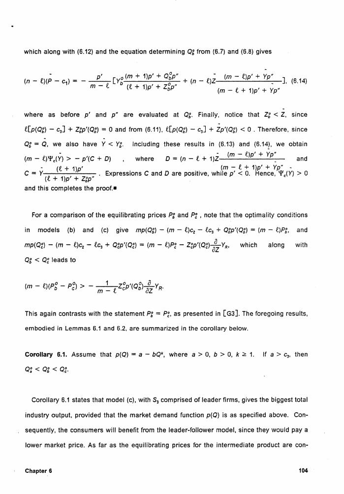
which along with (6.12) and the equation determining Qg from (6.7) and (6.8) gives

p' [YO (m + 1)p' + Qgp" (m - t)p' + Yp" b 0 + (n - t)Z-------J. (6.14)

m - t (t + 1)p' + Zbp" (m - t + 1)p' + Yp"

where as before p' and p" are evaluated at Qg. Finally, notice that Zg < Z, since

t[p(Qg) - c3] + Zgp'(Qg) = O and from (6.11), t[p(Qg) - c3] + Zp'(Qg) < O . Therefore, since

Qg = Q, we also have Y < Yg. Including these results in (6.13) and (6.14), we obtain

(m - t)'l'c(Y) > - p'(C + D) where D = (n - t + 1)Z-('-m_-_t-')p_'_+_Yp_"_ and (t + 1)p' (m - t + 1)p' + Yp" -

C = Y . Expressions C and D are positive, while p' < 0. Hence, 'l'c(Y) > 0 (t + 1)p' + Zgp" .

and this completes the proof.•

For a comparison of the equilibrating prices Pg and Pg , note that the optimality conditions

in models (b) and (c) give mp(Qg) - (m - t)c2 - tc3 + Qgp'(Qg) = (m - t)Pg, and

mp(Qg) - (m - t)c2 - tc3 + Qgp'(Qg) = (m - t)Pg - Zgp'(Qg) a~ YR, which along with

Qg < Qg leads to

This again contrasts with the statement Pg = Pg, as presented in [G3]. The foregoing results,

embodied in Lemmas 6.1 and 6.2, are summarized in the corollary below.

Corollary 6.1. Assume that p(Q) = a - bQk, where a > 0, b > 0, k ~ 1. If a > c3, then

o: < Qg < Qg.

Corollary 6.1 states that model (c), with S3 comprised of leader firms, gives the biggest total

industry output, provided that the market demand function p(Q) is as specified above. Con-

sequently, the consumers will benefit from the leader-follower model, since they would pay a

lower market price. As far as the equilibrating prices for the intermediate product are con-

Chapter 6 104

cerned, such a comparison is not straightforward. However, when the demand function p(Q)

is linear, i.e., k = 1, then using the results presented in Chapter 5, one can easily verify that

Po a - C3 pO a - C3 pO -- c + a - C3 a = C1 + - C + ------"---- -------'------n + 1 • b - 1 (n _ o + 1)(o + 1) · c 1 {, {, (n - i + 1)[ 1 + i(m - i + 1)]

By comparing the above prices, we obtain P~ > Pg > Pg. Hence, in this case, the downstream

stage also benefits by virtue of lower prices paid to the firms in S1, given that the vertically

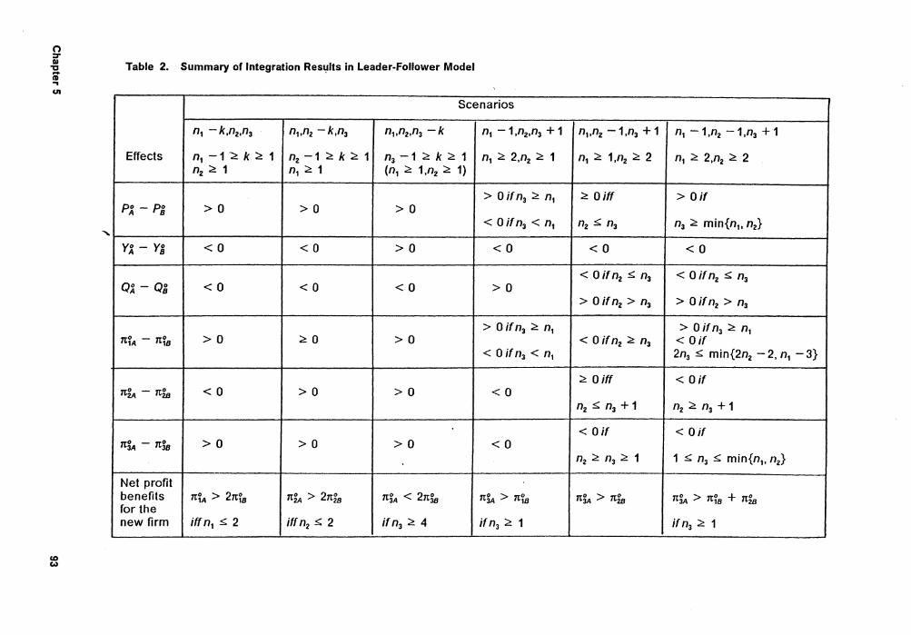
integrated firms act as leaders. However, as shown in Table 2, their profits decrease, which

may be due to the final commodity price decline.

To summarize, in this section three models were compared with respect to the total

equilibrating industry output. For a more thorough comparison, it would be required to also

consider profitability issues, which might give an interesting insight into benefits and losses

resulting from vertical integration and the types of interactions among the final commodity

suppliers. Such problems may be considered in terms of cooperative games, as suggested in

the next section.

6.2. Some Comments and Suggestions for Further Research

Models representing a two-stage industry were first considered by Greenhut and Ohta

[ G1 ].[ G3] in the context of benefits stemming from the vertical integration of firms in the

petroleum industry. Their analysis is sketchy and erroneous. However, they realize an alter-

nate way of approaching equilibrium concepts in such models. Green hut and Ohta ([ G1 ].p.

276) write:

"Given a demand function for a good, one may deduce a derived demand

function for, let us say, the intermediate good or service such as

transportation. This function would yield, in turn, another derived

demand function, for example, for the tires used by the carrier, and

so forth."

Chapter 6 105

The concept of the derived demand function has been extensively employed in the present

analysis, for the purpose of examining the existence of an equilibrium solution in the model

under various behavioral assumptions for the firms. In its derivation and characterization, a

mathematical programming-based approach for determining oligopolistic equilibria, plays a

key role. It was first introduced by Murphy et al. [M3]. in ttie context of a Nash-Cournot

equilibrium, and carried further by Sherali et al. [53] in the analysis of a Stackelberg type of

oligopoly.

The existence of an equilibrium solution, in the case of the follower-follower and the multiple

leader-follower behavior among the final product suppliers, and a perfect competition or

oligopolistic behavior in the upstream stage received much attention in our analysis. The de-

velopment was aimed at identifying those properties of the market demand function and the

cost functions of the firms in S1 U S2 U S3 which ensure the existence and uniqueness of an

equilibrium solution in the network. Furthermore, some computational techniques were pre-

sented, for determining an equilibrium solution, given the above market assumptions. Also,

some issues concerning various mergers and integrations among the producers are dis-

cussed herein, including changes in market price paid by the consumer and changes in profits

faced by each type of the producer.

Several issues remain that are not addressed in this research. One relates to the power

of the downstream producers in purchasing the semi-finished product. In our model, it is as-

sumed that the firms in S2 are price-takers, which may be justified in situations when there

are many downstream firms. However, in case of few downstream producers, they are likely

to actively participate in price formation for their input, and adopt oligopsonic behavior.

Analysis of a model which incorporates this type of behavior for the firms in S2, being a novel

study, would contribute to a more thorough insight into two-stage industries.

Another problem that might be interesting to look into, relates to the collusion of firms. In

this research, we were concerned with investigating changes in various quantities (e.g., total

industry output, firms profits ) that would take place if some firms decide to collude or inte-

grate, while the remaining producers continue to operate in the same manner as before such

Chapter 6 106

integration. In particular, the problem of the most profitable configuration for the firms was not

addressed here. Recently, these types of problems have been investigated by Sherali and

Rajan [S4] in the context of cooperative games, with players being some homogeneous

product suppliers. Sherali and Rajan attempt to determine what coalition, if any, would

emerge under three types of firms behavior. Accordingly, they analyze three games. In the

first game, each coalition assumes that the remaining firms will decide to do what is worst for

it. Two other games employ the concept of a Nash-Cournot equilibrium. In the second one,

each coalition assumes that its rivals will coalesce, so that a Cournot type of a duopoly will

result, while in the third one, they are assumed to remain separate Cournot firms. Conceptu-

ally, the third game is closely related to our collusion considerations. Using a linear demand

function and quadratic cost functions, identical for all, say n, producers, Sherali and Rajan

[S4] demonstrate that the grand coalition (i.e., total collusion) emerges for the first game. A

similar result is established for the third game, in case when n ~ 4. In contrast with this, the

grand coalition will not emerge in the second game, unless n = 2, and in particular, if n = 3

or n = 4, the best the firms can do is to remain separate. Similar questions can be addressed

in the context of a two-stage model. Such a study would not be easy, since as was mentioned

earlier, any change in the number of firms in S2 or in S3 imposes a new derived demand

function. Consequently, the task of determining the value of a coalition which involves the final

commodity suppliers is not trivial. However, by analyzing the simplified case of a linear de-

mand function and identical firms within each set S1, S2 and S3, one may be able to gain some

further insights into the problem of what types of configurations of firms would emerge in

two-stage models. Also, it would be interesting to conduct a similar analysis for a model which

incorporates oligopsonic behavior on the part of the downstream producers.

In the present analysis, the oligopolistic nature of the firms was based on either the Cournot

type of behavior or on Stackelberg's leader behavior. However, various definitions of an

equilibrium solution are conceivable, under various appropriate behavioral assumptions. One

such possibility incorporates the notion of consistent conjectures as addressed below. The

concept of consistent conj~ctures equilibrium is due to Bresnaham [81] who also derived

Chapter 6 107

conditions for its existence and uniqueness in the case of a duopoly. Here, the issue is to

ensure that at an equilibrium, the firm's behavior is consistent with its assumptions about the

other's behavior. In other words, at an equilibrium the slope of the reaction function should

be equal to its conjectural variation. The Cournot oligopoly yields inconsistencies. The firms

are right for wrong reasons, as concluded by Fellner. Each firm assumes zero conjectural

variations; however, its reaction function embodies a nontrivial relation between its

equilibrating output level and the equilibrating outputs of the remaining firms. In contrast with

this, the Stackelberg firm in a leader-follower duopoly, is known to be right for the right rea-

sons. Bresnaham [81] demonstrates that under some assumptions on the demand function

and the cost functions, the Bertrand duopoly also produces a consistent conjectures equilib-

rium.

Turning to our two-stage model, questions may be posed about the formulation and subse-

quently, about the the existence of a consistent conjectures equilibrium. First, what type of

conjectural variations would ensure that the final commodity suppliers are consistent in their

behavior, at least at an equilibrium ? Further, what conditions should be imposed to guaran-

tee that the equilibrating process among the firms in S2 U S3 produces a well behaved demand

function for the intermediate product? Would the final commodity consumers benefit from the

correctness of the firms' conjectures, as is the case of a (single market) duopoly? It can be

expected that mathematical programming concepts would facilitate the analysis in this case

as well.

Chapter 6 108

APPENDIX A

A.1. Proof of Theorem 3.8 (ii).

Below we establish strict concavity of <1>(0), for s e [O, Y0). Note that for this purpose, it is

sufficient to demonstrate that Y+(P) is strictly decreasing in P for Pe [O, Pa). that is over its

positive range. Recall that equation (3.23) states that

(A.1)

From Theorem 3.2 and 3.7, 0~ YR < 0, while z+(P) > O. Furthermore, since k > 1, we obtain

from Lemma 3.3 that ~YR is strictly decreasing in P for Pe [O, P0). This implies that for any oP

0 :s;: P1 < P2 < P0 we have y+(P2) < y+(P1) whenever z+(P1) = 0. Hence, in order to complete

the proof we need to show that y+(P) is strictly decreasing for those P < Pa for which

z+(P) > 0. Now, following the argument in Corollary 3.6, we conclude that Z;(P) = Z(P)/n3, .

i = 1, ... , n3, for all Pe [O, P0), and that if z+(P) > 0 for some P = P <Pa, then in (3.22), .

J 3(P) = {1, ... , n3}. This along with (3.14), (3.15) and (3.23), gives for Pe [O, Pa) . (for the sake

of notation we henceforth omit all the arguments):

(A.2)

(A.3)

APPENDIX A 109

(A.4)

where

V = (n2 + 1)p' + p"Y (A.5)

L = C + (n2 + k)Q 2 (A.6)

M = C + (n2 + k)DQ (A.7)

C = n3D2 + (k - 1)Z(O - Z) (A.8)

D = (n2 + k)Q - (k - 1)Z (A.9)

and where Q=Y+Z.

Letting G(P) denote the expression on the fight-hand side of (A.3) we need to show that

G +(P) < 0. Toward this end, denote the denominator in (A.3) by co(P). Then, by taking the

right-hand derivative of G(P) we get

+ D2h''[2p'p"Q+M + (p')2M+ - 2oo+vh" + 0 2v+h" - - 1-0 2Vh"'Z+] n3

Denote by K the sum of the first two terms on the right-hand side above, that is

APPENDIX A 110

and by H the sum of the remaining terms. In order to demonstrate that G + (P) < 0 it suffices

to show that H :s;; 0 and K < 0. In the proof we will employ the equations below, which readily

follow from the assumed form of the demand function p(Q) = a - bQk and expressions for V

and D introduced in (A.5) and (A.9):

(k - 1)p' = p"Q (A.10)

(k - 1)V = p"D (A.11)

(A.12)

(5.12a)

(A.13)

First, we will show that H < 0. By rearranging the terms we get

- p'Dh"(DVL + - 2Lo+v + 2p'D+M - p'DM+).

From (A.12a), since k > 1, , Q+ < 0, y+ < 0, we have v+ > 0. Hence, the first term in the

above expression of H is nonpositive. Therefore, since p' < O , z+ > 0, h" :<:: 0, h"' :s;; O (the

last result follows from the assumed concavity of h'(") , it remains to show that the bracketed

terms, denote them by 8 1, 8 2, 8 3 are all nonpositive. Consider 8 1 first. By (A.10) and (A.11)

we get 8 1 = LV - p'M = k ~ 1 p"(LD - QM) , and further, by (A.6), (A.7), 8 1 = p"C(D - Q).

Readily, 8 1 < 0, since p" < 0 and D > Q. Let us now proceed to 8 2• From equations (A.10),

(A.11) and (A.13) we obtain that 8 = - p"Q+Lv+ + p'LV + 2p'p"Q+M = 1 {p")2 2 (k - 1)2

[ - (k - 1)Q+Lo + (k - 2)Q+DL + QD+L + 2(k - 1)QQ+M]. But, QQ+M < O , since

APPENDIX A 111

Q+ < 0, and therefore, (k - 1)2B2 < (p")2L(QD+ - Q+D) . From equation (A.9) we get

QD+ - Q+D = (k - 1)(ZQ+ - QZ+) which along with Q+ < 0 and z+ > 0 gives

oo+ - o+o < o (A.14)

thus establishing B2 < 0. Now, let us show that 8 3 < O . Again, using (A.10) and (A.11) one

obtains

and further, by rearranging the terms, (k - 1)83 = p"[2D+(MQ - LD) + D(DL + - QM+)].

From (A.16) and (A.7), MQ - LD = C(Q - D) and DL + - QM+ = c+(D - Q)

+ (n2 + k)Q(DQ+ - D+Q) , which along with (A.14) and p" < 0 gives (k - 1)83 <

p"(D - Q)(c+o - 2o+C). Observe that c+o - 2o+c = (k - 1)(D - 2Z)(Dz+ - o+z) . But,

D - 2Z > (n2 + 1)0 - 2Z > o since n2 ~ 1, and oz+ - o+z > o since z+ > o and o+ < o. Therefore, c+o - w+c > o which along with p" < o and D > Q implies 8 3 < o. and hence

H < 0.

Now, we proceed to establishing K < 0. First, notice that from (A.10) the expression K can

be rewritten in the following way:

But, p" < 0 and therefore, K < 0 if and only if Q(L +M - LM+) - (k - 1)Q+LM is positive.

Toward this end, observe that from (A.8) and (A.9) we have

D+ = (n2 + k)Q+ - (k - 1)Z+

.c+ = Q+[2n3(n2 + k)D + (k - 1)(n2 + k)Z] + (k - 1)Z+[ - 2n3D + D - 2Z - (k - 1)Z].

APPENDIX A 112

By employing the above equalities in the expression for L +M - LM+ we obtain

K1 = (n2 + k)Q[2CQ + 2n3(n2 + k)D 2Q + (k - 1)(n2 + k)DQZ + 2(n2 + k)DQ2

- (k - 1)(n2 + k)Q2Z]

- (k - 1)[C2 + (n2 + k)CQ2 + (n2 + k)CDQ + (n2 + k)2DQ3],

and

K2 =: (k - 1)[ - 2n3D2 + D(D - 2Z) - (k - 1)DZ + C + (n2 + k)Q2 + 2n30Q

- Q(D - 2Z) + (k - 1)QZ].

Further, by equations (A.1) and (A.4) we can rewrite K in the following way:

Below we show that K1 - CK2 < 0 and K2 < 0 . Then, we will be able to claim that K < 0 since

co > O and p' < 0, h" s: 0. Toward this end,

K1 = (n2 + k)Q{2CQ + (n2 + k)Q[2n3D2 + (k - 1)DZ] - (n2 + k)Q2[2n3D + (k - 1)Z]

+ (n2 + k)OQ2 - CD - (n2 + k)CQ - (n2 + k)2Q3}

APPENDIX A 113

- (k - 1)[C2 + (n2 + k)CQ2 + (n2 + k)CDQ + (n2 + k)2DQ3] <

(n2 + k)(k - 1)CQ(Z - Q) - (k - 1)[C2 + (n2 + k)CDQ + (n2 + k)2DQ3].

The last inequality is valid through the following derivation:

2CQ + (n2 + k)Q[2n3D2 + (k - 1)DZ] - (n2 + k)Q2[2n3D + (k - 1)Z]

+ (n2 + k)DQ2 - CD - (n2 + k)CQ - (n2 + k)2Q3 =

2CQ + (n2 + k)Q[2C - (k - 1)Z(D - 2Z)] - (n2 + k)Q2[2n3D + (k - 1)Z]

+ (n2 + k)Q2[D - (n2 + k)Q] - CD - (n2 + k)CQ =

2CQ + (k - 1)CZ - (n2 + k)(k - 1)QZ(D - 2Z) - 2n3(n2 + k)Q2D - 2(n2 + k)(k - 1)Q2Z

< (k - 1)CZ + 2Q[C - n3(n2 + k)DQ]

= (k - 1)CZ + 2Q[ - n3(k - 1)ZD + (k - 1)Z(D -Z)]

= (k - 1)CZ + 2(k - 1)QZ( - np + D - Z) < (k - 1)CZ.

The above inequality for K1 demonstrates that K1 < O and moreover, since Z < Q that

K1 < - (k - 1)C2. Therefore, in order to show that K1 - CK2 < 0 it suffices to show that

K2 + (k - 1)C > 0. But,

K2 + (k - 1)C = (k - 1){2C + (D - 2Z)(D - Q) - [2n3D + (k - 1)Z]D

APPENDIX A 114

+ (nz + k)Q2 + [2n3D + (k - 1)Z]Q}

= (k - 1){2C + (D - 2Z)(D - Q) - [2C - 2(k - 1)Z(D - Z) + (k - 1)ZD]

+ (n2 + k)Q2 + [2n3D + (k - 1)Z]Q}

> (k - 1)Z(2D - 2Z - D) > 0.

Thus, K2 + (k - 1)C > 0 which gives K1 - CK2 < 0 and the proof is complete. •

A.2. Derivation od Results in the Last Column of Table 1 and of Table 2

In this section results in the last column of Table 1 and that of Table 2 are derived. Let us

recall that subsrcipts A and B refer to "after" and "before" integration, respectively. That is,

for the considered here vertical integratio11, B refers to n1, n2 and n3 firms in S1, S2 and S3, while

A refers to n1 - 1, nz - 1 and n3 + 1 firms in S1, S2 and S3• All n1, n2 and n3 are positive inte-

gers.

A.2.1.Derivation of Results in the Last Column of Table 1

Recall that in this case we are using d1 = dz = d3 = 0.

ROW 1. From (5.11), using (5.7), (5.9) and d1 = d2 = d3 = 0, we obtain

ROW 2. From (5.11), again using d1 =dz= d3 = 0, we get

APPENDIX A 115

which readily yields YX - YS < 0.

ROW 3. From (5.11), using (5.5), (5.7) and (5.9) and d1 = d2 = d3 = 0, we get

_ n1n2 + n3(n1 + 1)(n2 + n3 + 1) ]· (n1 + 1)(n3 + 1)

The numerator of the term in[·] above simplifies to n1(n2 + n3 + 1) - (n3 + 1)(n2 - 1). Hence,

in particular, if n1 ~ min{n2 - 1, n3 + 1}, then OX - OS > 0.

ROW 4. From (5.12), we obtain

n2(2n1 + 1)(n3 + 1) - n2nf - (n1 + 1)2(n3 + 1) =Do.~~~~~~~~~~~~~~~~-

(n2 + n3 + 1)nf (n1 + 1)2(n3 + 1)(n3 + 2)

Now, from the numerator in [·] above, if n1 ~ 2n2 - 1 , then n2(2n1 + 1)(n3 + 1)

- (n1 + 1)2(n3 + 1) ~ {n3 + 1)[n2{2n1 + 1) - 2n2{n1 + 1)] = - n2(n3 + 1) < 0, and so

1t~A - 1t~B < Q Similarly, if n1 ~ 2n3 + 3

Hence, if

n1 ~ min{2n2 - 1, 2n3 + 3}, then 7t~A - n~8 < 0.

ROW 5. Again from {5.12), we get

ROW 6. For the firms in S3, we get from (5.12) that

APPENDIX A 116

The numerator of the term in[·] above simplifies to n2(n3 + 1) - (n1 + 1){n3 + 1) - n1n2 which

is negative from the first two terms if n1 + 1 ~ n2, or from the first and third terms if

n1 ~ n3 + 1. Hence, if n1 ~ min{n2 - 1, n3 + 1}, we have 7t~A - 7t~8 < 0.

ROW 7. From (5.12), we obtain

Since n1{n3 + 2) + n2 - 1 ~ n1(n3 + 2), the numerator above, T, say, satisfies

n2 ~ n1 and n2 ~ n3 + 1. Therefore, if n2 ~ min{n1, n3 + 1} , then 7t~A - (7t~A + 7t~) > 0 , and

this completes the derivation of results in the last column of Table ·1. •

A.2.2.Derivation of Results in the Last Column of Table 2

ROW 1. From the development in Section 5.2, the equilibrating price P0 is given by

P0 = c3 - c2 + (a - c3)/N(n1 + 1) where N = n2n3 + n3 + 1. Therefore, the sign of the differ-

ence P~ - P& is the same as that of {n1 + 1)N - n1[ 1 + n2(n3 + 1)] . From this, it can be easily

verified that if n3 ~ n1 or n3 ~ n2 then P~ > P& thus completing this proof.

ROW 2. From (5.22) we have

n1n2 ]. (n1 + 1)(n2 + 1)(n3 + 1)

APPENDIX A 117

The numerator of the expression in [·] simplifies to - n1nl - (n3 + 1){nf + nl - 1) which is

negative since n1 :::: 2 and n2 :::: 2. Hence, YJ( - Ya < 0 .

ROW 3. From (5.24), we get

0 0 a - c3 [ (n1 - 1)(n2 - 1) + n1ni(n3 + 1)(n3 + 2) QA - Os= --- ---------------

b n1n2(n3 + 2)[ 1 + n2(n3 + 1)]

The numerator T of the term in [ ·] can be presented in the following way:

where M = 1 + n2(n3 + 1). Using the equation above it can be easily verified that if n2 .:;; n3

then T < 0 and so QJ( - 0§ < O . On the other hand, if n2 > n3 then the second term in [·] in

the expression for T is positive, and furthermore, since n2 :::: n3 + 1, we obtain

T > (n3 + 1)M[n1n2(n1 + 1)(n2 + 1)(n3 + 2) - (nf + 1)(nl + 1)] > 0 , and hence O~ - 0§ > 0

For the purpose of demonstrating the results in rows 4-7, let us present the expressions for

individual firm profits 7t7 for the firms in S1, i = 1, 2, 3 :

7to _ D .--1'---[ n2 + N(n1 + 1) ]2 3 - 0 (n2 + 1) (n1 + 1)(n3 + 1)N

APPENDIX A

(A.15)

(A.16)

(A.17)

118

where D0 = (a - c3) 2/b, and N = 1 + n3(n2 + 1).

ROW 4. From (A.15) we have that

n2 ]. (n1 + 1)2(n2 + 1)2(n3 + 1)N

Let T denote the numerator of the expression in [·] . Upon simplification we get

Since n2 ~ 2, we have nl - n2 - 1 ~ 1, which upon simple reduction gives

and further, with n3 ~ n1, T > nf(n~ - n2 - 1). The last result yields T > 0, since by assump-

tion n2 ~ 2 . Thus indeed, n3 ~ n1 implies that 7t~A - 7t~8 > 0 . For the case of

2n3 ~ min{2(n2 - 1), n1 - 3} , let us rewrite the expression Tin the following way:

where M = 1 + n2(n3 + 1). If n2 ~ n3 + 1, then from the equation above, we get

In order to show that T < 0 it suffices to demonstrate that the term in [ ·] on the right-hand

side of the last inequality is nonpositive. Toward this end, observe that this term is fess that

n~[(n1 + 1)(n3 + 1) - (n1 - 1)(n3 + 2)], which in turn is negative if n1 ~ 2n3 + 3. Summarizing,

APPENDIX A 119

we showed that if n2 ~ n3 + 1 and simultaneously, if n1 ~ 2n3 + 3, then nrA - nrs < 0. This

completes the derivation of the results in row 4.

ROW 5. From (A.16) the sign of n~ - 7t~ is the same as that of

(nl - 1)(n2 + 1)(n3 + 1) - nfn2(n3 + 2), being negative if n2 ~ n3 + 1.

ROW 6. From (A.17), it can be easily verified that the sign of n14 - n38 is the same as that

T, where

and where, as before, N = n3(n2 + 1) + 1, M = 1 + n2(n3 + 1). Observe that if n2 ~ n3 ~ 1

then (n2 + 1)(n3 + 1) - n2(n3 + 2)2 < 0 and also M ~ N. Therefore,

Consider the expression T1, say, in the first term [ ·] . Upon simplification, T1 = - n1n1(2n3 + 3) + (nl -·n1 - 1)(n3 + 1)2 , and furthermore, if n1 ~ n3, then we obtain

T1 s: nl( - nl - n3 + 1)- (n1 + 1)(n3 + 1)2, and hence, T1 < - n1nl if only n3 ~ 1. Next, con-

sider the second term [ ·] , say, T2, in the last inequality for T. Again, by rearranging the terms,

we get

Moreover, implies that

T2 < nl[(n1 + 1)(n3 + 1) + n1(n3 + 2)]. Using the above bounds for T1 and T2, we get the fol-

lowing inequality for T:

which along with M > n2(n3 + 1) gives

APPENDIX A 120

From this one can easily verify that T < 0. Thus we showed that 1 ~ n3 ~ min{n1, n2} implies

ROW 7. From (A.15). (A.16) and (A.17) we have

where N = n3(n2 + 1) + 1, M = 1 + n2(n3 + 1). Denoting by Tthe numerator of the expression

in {'}, we get that

+ nfM2{N[(n1 + 1)2(n2 + 1)2(n3 + 1)2 - nfn2(n3 + 2)2] - nl(n2 + 1)(n3 + 1)(n3 + 2)2}. To show

that T > 0 it suffices demonstrate that the expression in O. say, T1 is positive. Observe that

the term in [.] upon simplification is equal to nf[(nl + 1)(n3 + 1)2 + n2(nl - 2)]

and hence for we get

with and (n1 + 1)2 ~ 9, since gives

T1 > (n2 + 1)(n3 + 1)[nl(8nN + 5n3 - 4) + 9n3(n3 + 1)] > 0. Hence, if n3 ~ 2, then T1 > 0 . On

the other hand, if n3 = 1 then T1 = N{nf[4(nl + 1) - n2] + 4(2n1 + 1)(n1 + 1)2}

- 18nl(n2 + 1), and from this, since 4(nl + 1) - n2 ~ 3nl + 4, and N > n2 + 1, we obtain that

T1 > (n1 + 1)[4(8nf + 10n2 + 9) - 18nl] > 0. Summarizing, T1 > 0 if only n3 ~ 1 , and hence

n3 ~ 1 implies 7t3A > 7t~A + 7t~. Let us remark that if n3 = 0, then it may turn out that

7t8A < 7tfA + 7t~, as for example, if n1 = 3 and n2 = 10. In contrast to this example, n1 = 3,

n2 = 3, n3 = 0 yields 7t3A > 7trA + 7t~. This completes the derivation of results in the last col-

umn of Table 2. •

APPENDIX A 121

Appendix B

This Appendix contains figures illustrating various effects of vertical integrations in the

follower-follower and leader-follower models discussed in Chapter 5. The market demand

function is linear, and so are all the cost functions, being identical within each set S;,

i=1,2,3.

In comparison with results in Tables 1 and 2 (Chapter 5), the figures presented herein pro-

vide additional information on variations in individual firms' outputs and profits, total outputs

and the input price at equilibrium. In particular, they demonstrate that vertical integration may

result in a decrease of the total industry output, thus bringing losses to the final product con-

sumers.

Each curve shows changes in a given quantity based on an individually scaled set of data.

Notationally, Case 4 (5) denotes a scenario of successive conversion of firms from the set

S1 (S2) to firms of the type in S3, and corresponds to the fourth (fifth) column in Tables 1 and

2. Case 6 relates to a scenario of successive merger of one firm in S1 and one firm in S2 to form

a new vertically integrated firm in S3• This case corresponds to the sixth col_umn in Tables 1

and 2.

Appendix B 122

100 ~ \\ I' 12

90 I \ I 2 I ' I \

~ 2

\ \

80 I ~ \ \

I ~ I \

~ 2 70 \

\ 2 \ \

\ 2 ~ ' 2 (/) 60 \ '2 I- \

:J ~ '2_ 0..

I- \ '2 :J 0 50 ~ '2. .....J \ -a <(

~ '·:t_ :J

0 2. ~ ~ '2 0 l! 0 \ '2, z ss, 2..2..

~ ~2 ~ '2

30 ~ '2,2 '~ '.2.. 'l 2.

20 ~ ~ 3 2 '5._3 \

2 ~ \

10 ~'3.. ~ ~~ \\;'

5-.3. 0 $°3'-3-0--s-3 2

0 10 20 30 l! 0

NUMBER OF FIRMS IN S~

Legend: Symbol i refers to the firms in S1, i = 1,2,3.

Figure 2. Vertical Integration in Follower-Follower Model, Case 4.: Changes in Firms' Individual Outputs. n1 = 35 - na, n2 = 20, na = 1, ... ,34.

Appendix B 123

(/) I-:) Q_ I-

100

90

80

70

60

:) 50 0 --' ~ 0 I- 40

30

20

10

0

0 10 20 30 40

NUMBER OF FIRMS IN S~

Legend: Symbol i refers to the firms in S;. i = 2,3, Q refers to the total industry output.

Figure 3. Vertical Integration in Follower-Follower Model, Case 4.: Changes in Firms' Total Outputs. n1 = 35 - n3, n2 = 20 , n3 = 1, ... ,34.

Appendix B 124

100 ~\

\

90 ~~ I' 'I I \ 'I I

\1 I

11 ~ 80 \I \ I

,1 • ! \

~ ~ I I I 'I l

\ \ \ 70 :g I

w I\ I u I \ \ I I

D::'. 1 I Q_ I~ \

~ \ \

0 60 ~ z I \ <( \ I

(./) I I 2 I f- \ ~

\ \ I

c::: 50 I I 2 I 0 I \

D::'. \ 2 I

Q_ I ~ \ I _J \ 2 I

<( \ \

~ => 40 ~ ~ 2 0 \ I

~ I \ 2. I 0 \ ~ '2_ I

z I

~ 2 I

30 ~ '2,Q r \ ~ ""'g

I ~ 2.2 I 20 ~ ~ 2 F,O

I ~'\, 2 2 I ~ J 2 I

~ 2-2, r

~ 2-, 10 'R, ~'&_ 2,

3. ? 2. ~'R

.3~ 2 ~ P' ~ '0-3-3-3-J-3-}~ 0

P--p

0 10 20 30 40

NUMBER OF FIRMS IN S~

Legend: Symbol i refers to the firms in S;, i = 1,2,3, symbol Prefers to the input price.

Figure 4. Vertical Integration in Follower-Follower Model, Case 4.: Changes in Firms' Individual Profits and the Input Price. n1 = 35 - n3 , n2 = 20, n3 = 1, ... ,34.

Appendix B 125

(/) I-=> Cl.. I-=> 0 _J <( :::> 0 > 0 z

100

90

80

70

60

50

40

30

20

10

o

\ I \ \ \ \ \ \ I \ I \ \ \ I \ I \ ] I I I I \ \ I \

2 - - -2- - -~ - - -2 - - z:- --2- - -2- - - 2- - -2 - - -2- - - - -2- - -2:- - -2-- -2- -2- - -2- --2- - -2: \ \ \ \

3

\

~ \

\

~

5 7 9 11 13 15 17 19

NUMBER OF FIRMS IN S3

Legend: Symbol i refers to the firms in S;, i = 1,2,3.

Figure 5. Vertical Integration in Follower-Follower Model, Case 5.: Changes in Firms' Individual Outputs. n1 = 35, n2 = 20 - n3, n3 = 1, ... ,19.

Appendix B 126

(/) f--::J Q_ f--::J 0 _J

~ 0 f--

100 2 o---0- -0---:0 \ \

\ _...Q-0-Q- / '2 \

__.() J \ A'» / 90 \

~ , ;;r z/ \ ,o/ /

\ /

2 /if' ;t \

80 ' / \ f1 /

\

.2. , ;s rj\ /

/

70 I ~ J \

\ /

rj ' '!;/ 2 \ I

I ' / \

60 I '2 ;t '

/ I \ /

f/J 2- ;5 J \ /

I \ / 50 \~

I I '

I / \

·z/ '

I I '2 /

\

40 ' J ;5 \

¢ I 2-/ ' \

I ;5 \

2 30 I I \

I / \

/) \

I 'z I / \

~I \

\

I 2-20 I I / \

I z \

I \

/ 2 I I

\ \

I ;5 \

10 '9 I /

....._

I / \

;5 \

I '2 // ' \

' 0 @

\

2

3 5 7 9 1 1 13 15 1 7 19

NUMBER OF FIRMS IN S~

Legend: Symbol i refers to the firms in S;, i = 2,3, Q refers to the total industry output.

Figure 6. Vertical Integration In Follower-Follower Model, Case 5.: Changes in Firms' Total Outputs. n1 = 35, n2 = 20 - n3, n3 = 1, ... ,19.

Appendix B 127

100

90

80

70 w u 0::: CL 0 60 z <( (/) t-LL: 50 0 0::: CL _J <( ~ 40 0 > 0 z

30

20

10

2- - -2- - -2- - -2:- -z- --2- - -2- - - z- --2- --2- - -2- - -2 - - ~- _-:: 0

1 3 5 7 9 11 13 15 1 7 19

NUMBER OF FIRMS IN S3

Legend: Symbol i refers to the firms in S;. i = 1,2,3, symbol P refers to the input price.

Figure 7. Vertical Integration in Follower-Follower Model, Case 5.: Changes in Firms' Individual Profits and the Input Price. n1 = 35, n2 = 20 - n3, n3 = 1, ... , 19.

Appendix B 128

(/) I-::> 0.... I-::> 0 _J <( ::> 0 ~ 0 z

100

90·

80

70

60

50

40

30

20

10

0

0

~ -2-2-2 £-2-2-2-2-2 I 2.-.3-2-2-2 I -2-2-2 a I -c-2-a I z.-a I z.,2, I 2~ I '.2_ I 2 I ' I 2 I ' I 2 I I

I '

I * I ' I \

~ ~ I I I I

I \ I

' \ \

~ I \ I I 1i I I I 1i

\ ]

\

'.\ ~\ ~ ~ ~~

'3--:

I I I I

~

I I I I I I I

1? ~~- ~~

~-0-~~~~~3~~~~ 2

10 20 30

NUMBER OF FIRMS IN S~

Legend: Symbol i refers to the firms in S;, i = 1,2,3.

40

Figure 8. Vertical Integration in Follower-Follower Model, Case 6.: Changes in Firms' Individual Outputs. n1 = 35 - n3, n2 = 40 - n3, n3 = 1, ... ,34.

Appendix B 129

100 2 _ .Q-GQ-0 ~Q-OQ-E/-0-Q~ l) \

2 .Q-<fi8 i '2. ,e-0 i () 90 '2, r/1~ i ~

2, rJ i 80 ~: i

I 2. i ~ ~ t

~ '2, ;5 70 I 2 ;5 I '2 ¢ ~ ? , ~ J 60 I '2, i"l> (/) I

t- ¢ ~\~ i ~ Cl.. t- I );5 ~ 50 0 I

_J I ? 2, <{ I 2 t- I l) '2 0 t- 40 , '!J '

~ i 2, i ~ I ;5 1, ,

30 I ;3 2, , J 2, I 3 2. I i 'z 20 I I i '2. I t ~ I ;5 '~

10 I , ;5 '2 115 \

I 2 /} ' \

0 0 2

0 10 20 30 40

NUMBER OF FIRMS IN S~

Legend: Symbol i refers to the firms in S;. i = 2,3, Q refers to the total industry output.

Figure 9. Vertical Integration in Follower-Follower Model, Case 6.: Changes in Firms' Total Outputs. n1 = 35 - n3, n2 = 40 - n3 , n3 = 1, .. .,34.

Appendix B . 130

100 i-Q-2-2-2-2-~~-2~£-2-2.z I -2-," 2-2:'.

90 '2 '22

\ 2~~ 80 I ~~

' 2

\ \

70 ~ w I u

\ I

0::: 2 n.. I I

0 60 I

z I I

<( ~ (/)

\ I

I-CL 50 0 0::: 0..

\ _J <( :;, 40 0 > 0 I

I z ~

I

30 I I

2

" I

~ I 20 r \~~ I r

~~ I

J 10 p3'3.. p~ ' 3-R.p -3 '3-_3-: ,µ

0 'Rp'-8 3-J..3-3 3-3-3-3-~'3~-3~ 1

0 10 20 30 40

NUMBER OF FIRMS IN S~

Legend: Symbol i refers to the firms in S;. i = 1,2,3, symbol P refers to the input price.

Figure 10. Vertical Integration in Follower-Follower Model, Case 6.: Changes in Firms' Individual Profits and the Input Price. n1 = 35 - n3 , n2 = 40 - n3, n3 = 1, .. .,34.

Appendix B 131

20

10

~ CJ:'.: i.:L 3: w z <( u... 0 0 (/) I-G:: w z w l'.Il

ti z

-10

-20

0 10 20 30 40

NUMBER OF FIRMS IN S~

Legend: Symbol * refers to the net profit benefits of a new firm.

Figure 11. Vertical Integration in Follower-Follower Model, Case 6.: Net Profit Benefits of a New Firm. n1 = 35 - n3, n2 = 40 - n3, n3 = 1, ... ,34.

Appendix B 132

(/) I-~ Q_ I-~ 0 _J <( ~ 0 ~ 0 z

100

90

80

70

60

50

40

30

20

10

0

0 10 20

NUMBER OF FIRMS IN S?J

Legend: Symbol i refers to the firms in S;. i = 1,2,3.

30 40

Figure 12. Vertical Integration in Leader-Follower Model, Case 4.: Changes in Firms' Individual Outputs. n1 = 35 - n3, n2 = 20, n3 = 1, ... ,34.

Appendix B 133

(/) I-~ Cl.. 1-

100

90

80

70

60

::> 50 0 _J

~ 0 I- L.lO

30

20

10

0

0 10 20 30 L.lO

NUMBER OF FIRMS IN s3

Legend: Symbol i refers to the firms in S;. i = 2,3, Q refers to the total industry output.

Figure 13. Vertical Integration in Leader-Follower Model, Case 4.: Changes in Firms' Total Out-puts. n1 = 35 - n3, n2 = 20, n3 = 1, ... ,34.

Appendix B 134

100

90

80

70 w u 0:::: Q_

0 60 z <{ (/) I-G::: 50 0 0:::: Q_ _J <{ :::> 40 0 > Ci z

30 I

I I

20 ~ I

' 10 / f?.P'

pp

0 ~3-b~

0 10 20 30 40

NUMBER OF FIRMS IN S3

Legend: Symbol i refers to the firms in S;. i = 1,2,3, symbol Prefers to the input price.

Figure 14. Vertical Integration in Leader-Follower Model, Case 4.: Changes in Firms' Individual Profits and the Input Price. n1 = 35 - n3, n2 = 20, n3 = 1, ... ,34.

Appendix B 135

(/) I-=> ()_ I-=> 0 _J <( ::::> 0 ~ 0 z

100

90

80

70

60

50

40

30

20

10

0

0

I

',I I

' \1

10 20

i 2

NUMBER OF FIRMS IN S3

Legend: Symbol i refers to the firms in S;. i = 1,2,3.

I I

I I

'l-I

I

2 I

I z

30

I I I I I I I

2 I I

I I I I I

I I I I I I I I I I I :;.

2

40

Figure 15. Vertical Integration in Leader-Follower Model, Case 5.: Changes in Firms' Individual Outputs. n1 = 20, n2 = 35 - n3, n3 = 1, ... ,34.

Appendix B 136

(/) I-,:) 0.. I-

100

90

80

70

60

,:) 50 0 __J

~ 0 I- 40

30

20

10

0

0

2 I

; ' I I

I J

10 20 30 40

NUMBER OF FIRMS IN S~

Legend: Symbol i refers to the firms in S;, i = 2,3, Q refers to the total industry output.

Figure 16. Vertical Integration in Leader-Follower Model, Case 5.: Changes in Firms' Total Out-puts. n1 = 20, n2 = 35 - n3, n3 = 1, ... ,34.

Appendix B 137

100 2 I I I I I I

90 I I I I I I

80

70 w ~ a::: Q._

0 60 z <( (/) I-c;: 50 0 a::: Q._ _J <( :::> 40 0 > 0 z

30

20

10

0

0 10 20 30 40

NUMBER OF FIRMS IN S3

Legend: Symbol i refers to the firms in S;, i = 1,2,3, symbol Prefers to the input price.

Figure 17. Vertical Integration in Leader-Follower Model, Case 5.: Changes in Firms' Individual Profits and the Input Price. n1 = 20, n2 = 35 - n3, n3 = 1, ... ,34.

Appendix B 138

100

90

80

70

(/) 60 I-

:::> Cl.. I-:::> 0

50 _J <( :::> 0 ~ 0 40 z

30

20

10

0

0 10 20 30 LI 0

NUMBER OF FIRMS IN S~

Legend: Symbol i refers to the firms in S;, i = 1,2,3.

Figure 18. Vertical Integration in Leader-Follower Model, Case 6.: Changes in Firms' Individual Outputs. n1 = 35 - n3, n2 = 40 - n3 , n3 = 1, ... ,34.

Appendix B 139

100 2 @-0 G-Oe-0-Q-Q-0-BOQ ~~3 J.a~ I

~~ ~J~.a-*~ ~ 90 f1 .l~ \ ~, r~

I I ~~ ~ I CfJ 2 80 I I 't I ¢ I I I

I } 70 ¢i

I I

2 / ' '\ 1$ 60 ~~I Vl \I I f-

::::> I I []_ 'ti f- .~ ::J 50 0

11~ _J

~ 'I ' 0 / / ~ f- 40 9, ~

~ \ I 30

f 2

\ \

I ~ \

2 20 '.z_

f 2

'2'2

I '2'2 10 -2-2 -2'2 2-

- 2-2-2-2-2 _

J 2-2-21:-2-2 . 0

-2-2-22-2

0 10 20 30 40

NUMBER OF FIRMS IN S~

Legend: Symbol i refers to the firms in S1, i = 2,3, Q refers to the total industry output.

Figure 19. Vertical Integration in Leader-Follower Model, Case 6.: Changes in Firms' Total Out· puts. n1 = 35 - n3, n2 = 40 - n3, n3 = 1, ... ,34.

Appendix B 140

100

90

80

I I

70 I w I

fd I ~ I a_ I 0 60 z < (/) t-G: so 0 ~ CL _J

< :::> L! 0 0 > 0 z

30

20

10

0

a 10 20 30 L! 0

NUMBER OF FIRMS IN S~

Legend: Symbol i refers to the firms in S1, i = 1,2,3, symbol Prefers to the input price.

Figure 20. Vertical Integration in Leader-Follower Model, Case 6.: .Changes in Firms' Individual Profits and the Input Price. n1 = 35 - n3 , n2 = 40 - n3, n3 = 1, ... ,34.

Appendix B 141

100

90

80

70 ~ Cl:'.: c;::: ~ 60 w z <( Li... 0 50 (/) I-CL w z 40 w m ~ z

30

20

10

0

0 10 20 30 40

NUMBER OF FIRMS IN S~

Legend: Symbol * refers to the net profit benefits of a new firm.

Figure 21. Vertical Integration in Leader-Follower Model, Case 6.: Net Profit Benefits of a New Firm. n1 = 35 - n3, n2 = 40 - n3, n3 = 1, ... ,34.

Appendix B 142

Bibliography

B1. Bresnahan, T. F. 1981. Duopoly with Consistent Conjectures. American Economic Review 71, 934 - 945.

C1. Cournot, A. A. 1838. Researches into the Mathematica/Princeples of the Theory of Wealth. Translated by Nathaniel T. Bacon. 1927. New York: Macmilan.

F1. Frank, Ch. R. Jr. and R. E. Quandt. 1963. On the Existence of Cournot Equilibrium. Inter-national Economic Review 4 , 92-96.

F2. Friedman, J. W. 1977. Oligopoly and the Theory of Games. Amsterdam :North-Holland.

F3. Friedman, J. W. 1983. Oligopoly Theory. New York: Cambridge University Press.

F4. Friedman, J. W. 1986. Game Theory with Applications to Economics. New York: Oxford University Press.

F5. Furth, D. 1979. The Stability of Generalized Stackelberg Equilibria in Heterogeneous Oligopoly. Journal of Economics 39, 315-322.

G1. Greenhut, M. L. and H. Ohta. 1976. Related Market Conditions and lnterindustrial Mergers. American Economic Review. 66, 267-277

G2. Greenhut, M. L. and H. Ohta. 1978. Related Market Conditions and lnterindustrial Mergers: Reply. American Economic Review. 68, 228-230.

G3. Greenhut, M. L. and H. Ohta. 1979. Vertical Integration of Successive Oligopolies. Amer-ican Economic Review. 69, 137-141.

H1. Haring, J. R. and D. L. Kaserman. 1978. Related Market Conditions and lnterindustrial Mergers: Comment. American Economic Review. 68, 225-227.

M1. MacKinnon, J. 1977. Solving Economic General Equilibrium Models by the Sandwich Method. In Fixed Point. Algorithms and Applications. Ed. S Karamardian in collaboration with C.B. Garcia. Academic Press, Inc., 367-402.

M2. McManus, M. 1962. Numbers and Size in Cournot Oligopoly. Yorkshire Bulletin of Social and Economic Studies 29, 14-22.

M3. Murphy, F. H., H. D. Sherali and A. L. Soyster. 1982. A Mathematical Programming Ap-proach for Determining Oligopolistic Market Equilibrium. Mathematica/ Programming 24, 92-106.

Bibliography 143

N1. Nash, J. 1951. Non-cooperative Games. Annals of Mathematics 54, 286-295.

N2. Nishimura, K. and J. W. Friedman. 1981. Existence of Nash Equilibrium in n Person Games without Quasiconcavity. International Economic Review 22, 637-648.

N3. Novshek, W. 1984. Finding of All n-Firm Cournot Equilibria. International Economic Review 25, 61-70.

01. Okuguchi, K. 1976. Expectations and Stability in Oligopoly Models. (lecture Notes in Economics and Mathematical Systems, No. 138). Springer-Verlag, New York.

02. Okuguchi, K. 1978. The Stability of Price Adjusting Oligopoly with Conjectural Variations. Journal of Economics 38, 50-60.

P1. Perry, M. K. 1978. Related Market Conditions and lnterindustrial Mergers: Comment. American Economic Review. 68, 221-224.

R1. Rovinsky, R. B., C. A. Shoemaker and M. J. Todd. 1980. Determining Optimal Use of Re-sources Among Regional Producers using Different Levels of Cooperation. Operations Research 28, 859-866.

R2. Ruffin, R. J. 1971. Cournot Oligopoly and Competitive Behavior. Review of Economic Studies 38, 492 - 502.

S1. Salant, S. W., S. Switzer and R. J. Reynolds. 1983. Losses from Horizontal Merger: The Effects of an Exogeneous Change in Industry Structure on Cournot-Nash Equilibrium. The Quarterly Journal of Economics 98, 185-199.

S2. Scarf, H. 1973. The Computation of Economic Equilibria . Yale, New HAven.

S3. Sherali, H. D. 1984. A Multiple Leader Stackelberg Model and Analysis. Operations Re-search 32, 390-400.

S4. Sherali, H. D. and R. Rajan. 1986. A Game Theoretic-Mathematical Programming Analysis of Cooperative Phenomena in Oligopolistic Markets. Operations Research 34, 683-697.

SS. Sherali, H. D., A. L. Soyster and F. H. Murphy. 1983. Stackelberg-Nash-Cournot Equilibria: Characterizations and Computations. Operations Research 31, 253-276.

S6. Stackelberg, H. 1934. Marktform und Gleichgewicht. Julius Springer, Vienna.

S7. Szidarovszky, F. and S. Yakowitz. 1977. A New Proof of Existence and Uniqueness of the Cournot Equilibrium. International Economic Review 18, 787-789.

S8. Szidarovszky, F. and S. Yakowitz. 1982. Contributions to Cournot Oligopoly Theory. Jour-nal of Economic Theory 28, 51-70. ·

. W1. Waterson, M. 1982. Vertical Integration, Variable Proportions and Oligopoly. The Eco-nomic Journal 92, 129-144.

Bibliography 144

The vita has been removed from the scanned document


Recommended