Page 1
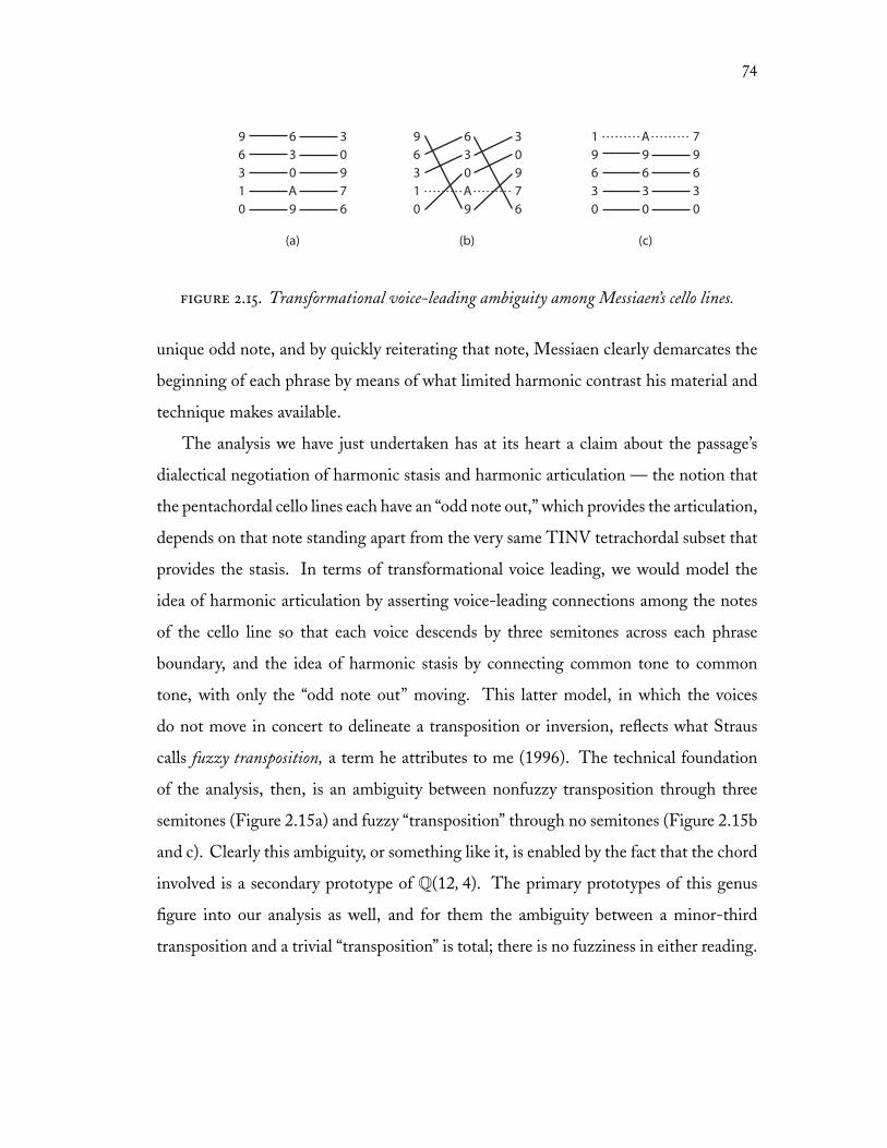
A Unified Theory of Chord Quality in Equal Temperaments
by
Ian Quinn
Submitted in partial fulfillment of the
requirements for the degree
Doctor of Philosophy
Supervised by
Professor Robert Morris
Department of Music Theory
Eastman School of Music
University of Rochester
Rochester, New York
2004
Page 2
ii
To the memory of David Lewin
Page 3
iii
curriculum vitæ
Ian Quinn was born at Warner-Robins AFB in Georgia on 19 March 1972. He was
awarded the B.A. in music from Columbia University in 1993. After studies in the
Ph.D. Program in Music at the CUNY Graduate Center under a Robert E. Gilleece
Fellowship, he came to Eastman in 1996 with a Robert and Mary Sproull Fellowship
from the University of Rochester, and was named Chief Master’s Marshal in 1999,
having earned the M.A. in October 1998. In that same year he won the Edward Peck
Curtis Award for Excellence in Teaching by a Graduate Student. He has held teaching
assistantships at Eastman and instructorships both at Eastman and at the University of
Rochester’s College Music Department. He left residence at the University to take the
first postdoctoral fellowship in music theory at the University of Chicago (2002–03)
and, subsequently, faculty appointments at the University of Oregon (2003–04) and
Yale University (from 2004). He has performed on Nonesuch and Cantaloupe Records
with Ossia, an ensemble he cofounded in 1997 that continues to play an active role in
the new-music scene at Eastman. His research as a graduate student has been presented
at many conferences and published in Music Theory Spectrum, Music Perception, and
Perspectives of New Music.
Page 4
iv
acknowledgements
The work presented here has been ongoing for ten years, during which time I have
benefitted from conversations with many people who have left indelible marks on the
final product. Jonathan Kramer gave me a bad grade on an analysis paper in 1993;
thinking about his remarks led me eventually to the fuzzy approach, which J. Philip
Lambert and Joseph Straus indulged during my years at CUNY. At Eastman I was
fortunate enough to meet Norman Carey, Gavin Chuck, Daniel Harrison, Panayotis
Mavromatis, Richard Randall, Damon Scott, and Virginia Williamson, all of whom
have engaged me in thought-provoking conversation and collaboration. Soon after my
arrival at Eastman, Peter Silberman organized a symposium on fuzzy-set theory at which
he, Brian Robison, and I shared our findings with each other and our colleagues; this
symposium encouraged me to continue thinking fuzzily, even after I thought I wasn’t
doing so any more. (Henry Kyburg of the University’s Department of Philosophy put
me back on track in a course with the inimitable title “Deviant Logic.”)
As a result of a session at the Southeast Sectional Meeting of the American Math-
ematical Society organized in 2003 by Robert Peck, I had the opportunity to fine-tune
many of these ideas after conversing with Clifton Callender, David Clampitt, Jack
Douthett, Julian Hook, John Rahn, and Ramon Satyendra.
The support of the Department of Music of the University of Chicago in the form
of a “postdoctoral” fellowship, which both underwrote the final phase of work and gave
me a delightfully rich intellectual environment to do it in, is warmly acknowledged.
Richard Cohn, whose unflagging support of my research has been indispensable, was
responsible for bringing the fellowship about; may his forward thinking be a model for
our field. My work is the better for conversation with my Chicago colleagues Lawrence
Page 5
v
Zbikowski and Jose Antonio Martins, as well as with the department’s brilliant graduate
students.
Special thanks are due to the members of my dissertation committee, Norman
Carey, Ciro Scotto, and Joseph Straus. Joe deserves special mention, since he provided
important guidance many years ago at CUNY when I was first forming some of these
ideas, and has been a steadfast mentor and supporter ever since; at a crucial stage he was
generous enough to put a draft on the reading list for his workshop at the 2003 Institute
for Advanced Studies in Music Theory at Mannes, from which much fruitful discussion
emerged, especially with Michael Buchler and Janna Saslaw; I was also happy to meet
my faithful correspondent Dmitri Tymoczko at Mannes.
At various other times and places, I have had good conversations — with Joseph
Dubiel, Eric Isaacson, Steve Larson, Art Samplaski, and Ramon Satyendra, among
many others — that have had a direct impact on this work. In addition to those already
mentioned, Trey Hall, Nigel Maister, Michael Phelps, Annalisa Poirel, Ben Schneider,
Omri Shimron, Jocelyn Swigger, and my parents (Quinn and Kent McDonald, and John
Quinn and Peter Grant) have provided vast amounts of moral support at appropriate
times. At the very end, Leigh VanHandel and I kept one another’s noses to a grueling
grindstone of daily “dissertation time,” constantly battling the Law of Conservation of
Productivity.
My advisor, Robert Morris, brought me to Eastman even though I accused him
of being a Cartesian, and is now letting me go even though he accuses me of being
a Platonist (he’s right; I was wrong). Throughout the intervening years we have
continually “misunderstood” each other as part of a wonderful dialectic I sincerely hope
will continue for many years.
This dissertation would not have been possible without David Lewin’s inspiration
and encouragement. In November 2002, days after having the idea that his very first
article contained the seeds of the fruit I had been foraging all these years, I excitedly
wrote him about it; his response was simply “Yes, I enjoy thinking about [that] too.”
Hoping he would live long enough to tell me whether I was thinking about it in the
Page 6
vi
right way once I’d fleshed out that idea, I waited too long to ask. So it’s with deep
sadness, and more than the usual humility, that I add the boilerplate disclaimer: any
remaining errors are entirely my responsibility.
Page 7
vii
abstract
Chord quality — defined as that property held in common between the members of
a pcset-class, and with respect to which pcset-classes are deemed similar by similarity
relations (interpreted extensionally in the sense of Quinn 2001) — has been dealt
with in the pcset-theoretic literature only on an ad hoc basis. A formal approach
that generalizes and fuzzifies Clough and Douthett’s theory of maximally even pcsets
successfully models a wide range of other theorists’ intuitions about chord quality, at
least insofar as their own formal models can be read as implicit statements of their
intuitions. The resulting unified model, which can be interpreted alternately as (a) a
fuzzy taxonomy of chords into qualitative genera, or (b) a spatial model called Q-space,
has its roots in Lewin’s (1959, 2001) work on the interval function, and as such has
strong implications for a unification of general theories of harmony and voice leading.
Page 8
viii
table of contents
Introduction 1
1 Theoretical background 4§ 1.1 Theorizing about categories. . . . . . . . . . . . . . . . . . . . . . 8§ 1.2 The intervallic approach to chord quality. . . . . . . . . . . . . . . 12
1.2.1 Prototypes. . . . . . . . . . . . . . . . . . . . . . . . . . . . 131.2.2 Intrageneric affinities. . . . . . . . . . . . . . . . . . . . . . . 191.2.3 Intergeneric affinities. . . . . . . . . . . . . . . . . . . . . . . 23
§ 1.3 Other approaches to chord quality. . . . . . . . . . . . . . . . . . . 271.3.1 The inclusional approach. . . . . . . . . . . . . . . . . . . . . 271.3.2 Morris’s algebraic approach. . . . . . . . . . . . . . . . . . . 311.3.3 Cohn’s cyclic approach. . . . . . . . . . . . . . . . . . . . . . 38
2 A unified theory of generic prototypes 43§ 2.1 Maximally even subgenera. . . . . . . . . . . . . . . . . . . . . . . 44§ 2.2 Against the Intervallic Half-Truth. . . . . . . . . . . . . . . . . . . 49
2.2.1 Examples. . . . . . . . . . . . . . . . . . . . . . . . . . . . . 492.2.2 Argument. . . . . . . . . . . . . . . . . . . . . . . . . . . . . 55
§ 2.3 Generalizing up to generic prototypes. . . . . . . . . . . . . . . . . 59§ 2.4 On theoretical unification . . . . . . . . . . . . . . . . . . . . . . 67
2.4.1 The story so far. . . . . . . . . . . . . . . . . . . . . . . . . . 672.4.2 A non-intervallic characterization of interval content. . . . . . 682.4.3 Harmony and voice leading. . . . . . . . . . . . . . . . . . . 71
3 A generalized theory of affinities 76§ 3.1 Fourier balances . . . . . . . . . . . . . . . . . . . . . . . . . . . . 77
3.1.1 Lewin’s five Fourier Properties. . . . . . . . . . . . . . . . . . 773.1.2 Completing and generalizing the system. . . . . . . . . . . . . 833.1.3 Fourier balances and qualitative genera. . . . . . . . . . . . . 85
§ 3.2 From prototypes to intrageneric affinities . . . . . . . . . . . . . . 883.2.1 Fuzzification. . . . . . . . . . . . . . . . . . . . . . . . . . . 883.2.2 Theoretical fallout. . . . . . . . . . . . . . . . . . . . . . . . 93
§ 3.3 Notes on Q-space. . . . . . . . . . . . . . . . . . . . . . . . . . . 100
Bibliography 108
Page 9
ix
list of figures
1.1 Algorithmic description of Hanson’s projection procedure. . . . . . . . 141.2 Hanson’s projections; tentative prototypes of the qualitative genera
Q(12, n). . . . . . . . . . . . . . . . . . . . . . . . . . . . . . . . . . 151.3 Figure 1.1 from Headlam (1996). . . . . . . . . . . . . . . . . . . . . 161.4 Eriksson’s maxpoints. . . . . . . . . . . . . . . . . . . . . . . . . . . 181.5 The “supermaxpoints.” . . . . . . . . . . . . . . . . . . . . . . . . . 191.6 Models of relative ic multiplicity in Eriksson’s seven “regions” (genera). 191.7 Eriksson’s graphic representation of his genera. . . . . . . . . . . . . . 231.8 Multiplication by 2 as an epimorphism. . . . . . . . . . . . . . . . . . 251.9 Harrison’s N operator. . . . . . . . . . . . . . . . . . . . . . . . . . . 261.10 Morris’s algebraic SG(3) genera (rows) versus qualitative genera (columns). 331.11 M5 structures certain intergeneric affinities; it also preserves certain
intrageneric affinities. . . . . . . . . . . . . . . . . . . . . . . . . . . 341.12 Morris’s nonstandard operators. . . . . . . . . . . . . . . . . . . . . . 371.13 Cohn’s CYCLE homomorphisms as multiplicative operators. . . . . . 391.14 Adapted from Cohn (1991), Table 5. . . . . . . . . . . . . . . . . . . 40
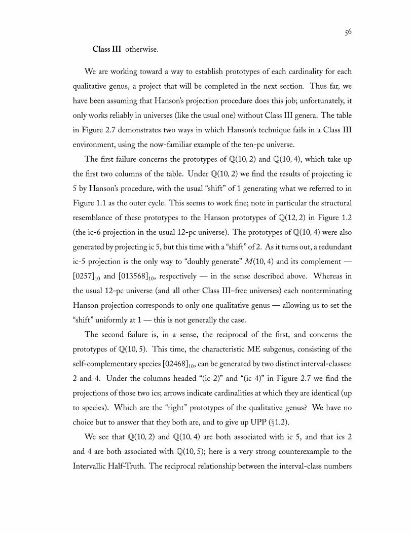
2.1 Classification of all ME species for c > 1 and 0 < d < c. . . . . . . . 482.2 The species M(c, d) for c = 11. . . . . . . . . . . . . . . . . . . . . . 502.3 The species M(c, d) for c = 12. . . . . . . . . . . . . . . . . . . . . . 512.4 The species M(c, d) for c = 10. . . . . . . . . . . . . . . . . . . . . . 522.5 Class III ME chords can be split into gcf(c, d) repeated “copies” of some
nontrivial Class I chord. . . . . . . . . . . . . . . . . . . . . . . . . . 532.6 ME subgenera and aligned subuniverses. . . . . . . . . . . . . . . . . 542.7 The failure of projection in universe with ME chords of Class III. . . . 572.8 Intervallic Half-Truth counterexamples from the 21-pc universe . . . . 582.9 Hanson’s projection procedure generalized. . . . . . . . . . . . . . . . 592.10 Tertiary prototypes in the twelve-pc universe. . . . . . . . . . . . . . 662.11 Interval content of primary Q(12, 1) prototypes. . . . . . . . . . . . . 692.12 Interval content of primary Q(12, 5) prototypes. . . . . . . . . . . . . 692.13 Interval content of other primary prototypes in the twelve-pc universe. 712.14 Analysis of the first few bars of Messiaen’s “Quatuor,” vii. . . . . . . . 732.15 Transformational voice-leading ambiguity among Messiaen’s cello lines. 74
Page 10
x
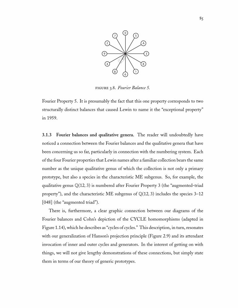
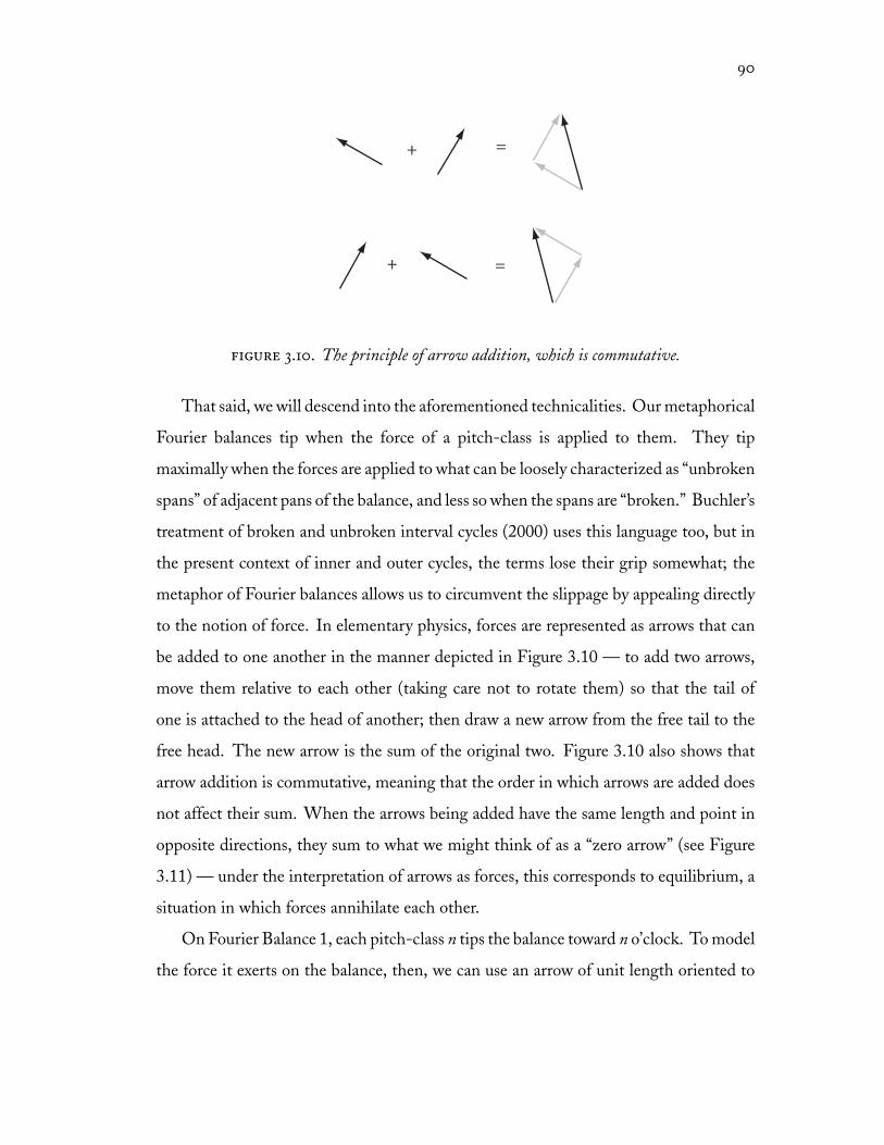
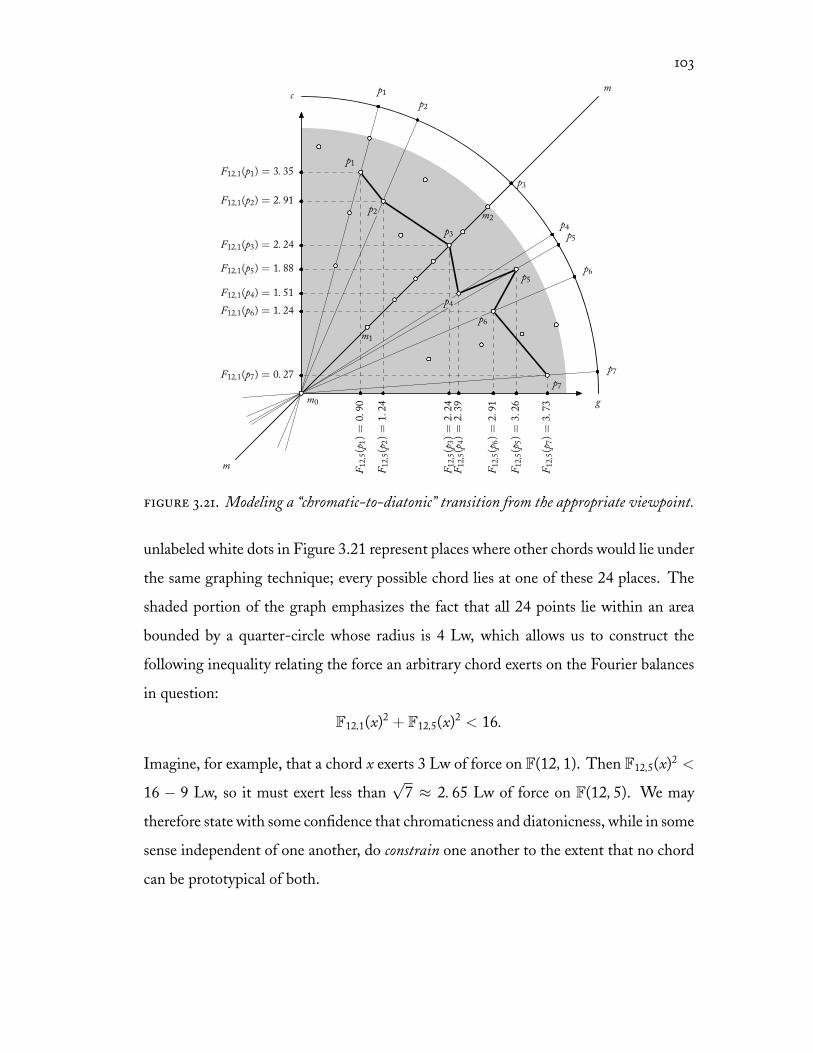
3.1 Lewin’s 1959 and 2001 names for the Fourier properties. . . . . . . . 783.2 Fourier Balance 6. . . . . . . . . . . . . . . . . . . . . . . . . . . . . 783.3 Fourier Balance 4. . . . . . . . . . . . . . . . . . . . . . . . . . . . . 803.4 Fourier Balance 3. . . . . . . . . . . . . . . . . . . . . . . . . . . . . 803.5 Lewin’s later model for Fourier Property 2. . . . . . . . . . . . . . . . 813.6 Fourier Balance 2. . . . . . . . . . . . . . . . . . . . . . . . . . . . . 823.7 Fourier Balance 1. . . . . . . . . . . . . . . . . . . . . . . . . . . . . 833.8 Fourier Balance 5. . . . . . . . . . . . . . . . . . . . . . . . . . . . . 853.9 Left to right: F(11, 5), F(10, 2), F(10, 4). . . . . . . . . . . . . . . . . 873.10 The principle of arrow addition, which is commutative. . . . . . . . . 903.11 Two mutually inverse arrows sum to a zero arrow. . . . . . . . . . . . 913.12 Association of arrows with Fourier Balance 1. . . . . . . . . . . . . . 913.13 Decomposition of a chord with Fourier Property 1 into arrow cycles. . 923.14 F12,1 for highly prototypical pentachords. . . . . . . . . . . . . . . . . 933.15 F12,4 for Messiaen’s prototypes. . . . . . . . . . . . . . . . . . . . . . 933.16 Measuring and approximating F12,1 for tetrachord types. . . . . . . . . 963.17 Hexachord species with high ic-4 content. . . . . . . . . . . . . . . . 983.18 Additional relationships among the species in Figure 3.17. . . . . . . . 993.19 Ligeti, Lux aeterna, beginning of first microcanon . . . . . . . . . . . 1003.20 Ligeti, Lux aeterna (opening): harmonic states at downbeats. . . . . . 1023.21 Modeling a “chromatic-to-diatonic” transition from the appropriate
viewpoint. . . . . . . . . . . . . . . . . . . . . . . . . . . . . . . . . 1033.22 Modeling increasing “chromaticness” necessitates a different viewpoint. 1063.23 One progression, two viewpoints. . . . . . . . . . . . . . . . . . . . . 107
Page 11
1
introduction
The commonplace notion that a sonority can be “closely” or “distantly” related to other
sonorities evokes a metaphorical space, in which individual sonorities are distributed
according to what we will chord quality. Closely and distantly related sonorities are
literally close to and distant from one another, respectively, in such a space; a sonority’s
quality can be defined as its location in that space. From a theoretical point of view,
an understanding of the nature of chord quality might take the form of a description
of that space’s structure and the laws that determine a sonority’s position. This is our
main goal; we will refer to the space as Q-space.
I have shown elsewhere (Quinn, 2001) that the various numerical models generally
characterized as pcset-class similarity relations agree with each other to a high degree,
despite major differences in their internal workings. In the present context, it is helpful
to think of the numbers put out by similarity relations as estimates of distances between
sonorities in Q-space. This approach accounts both for the agreement among various
similarity relations (since they are, in principle, estimating distances in a single space)
and for their failure to converge completely with one another (since each is only an
estimate).
Likewise, it is not difficult to conceive of the pcset-theoretical tools that produce
taxonomic categories superordinate to the pcset-class as modeling structural features
of Q-space. We might expect, for instance, that the pcsets belonging to a single one
of Forte’s genera (1988) would lie near one another in Q-space, and that the system
of genera as a whole can be viewed as a system of overlapping regions in Q-space.
The same could be said of Forte’s pcset-complexes (1973), of any of Morris’s set-group
systems (1982), or of Hanson’s categories (1960). Again, the spatial metaphor can be of
Page 12
2
assistance in understanding the nature of the differences among all of these systems. For
an example of the different ways in which it is possible to describe different regions in
the same underlying space, one need only consider the significant ways in which the map
of Europe changed over the course of the twentieth century — centuries-old villages in
(say) Macedonia or Transylvania have been incorporated into many different states and
spheres of influence without significantly changing certain “natural” and “transcendent”
national properties of those villages. Such properties tend to be shaped primarily by
permanent geographical features such as bodies of water, deserts, or mountain ranges.
In Chapter 1 we will survey the approaches of Hanson, Forte, Morris, and many
others, and see that certain well-known sonorities (e.g., the diatonic and pentatonic
collections, Messiaen’s modes of limited transposition, the hexatonic scale) turn up as
what we will call prototypes — highly characteristic sonorities, relative to which the
quality of other sonorities is determined. As such, these prototypical sonorities can be
thought of as sitting atop the mountains of Q-space, of which we will see that there are
six, roughly corresponding to the six interval classes of twelve-tone equal temperament.
Scattered around the slopes of these mountains are other sonorities more or less close to
the prototypes atop nearby peaks. What we are referring to here as a mountain will be
called, more technically, a qualitative genus, defined as a taxonomic entity characterized
by prototypical sonorities and encompassing sonorities to variying degrees, according
to their closeness to the prototypes. The closeness or distance of an arbitrary sonority
to the prototypes of a qualitative genus will be described in terms of the intrageneric
affinities of the genus, and abstract structural relationships among genera will be called
intergeneric affinities.
Chapter 2 will be concerned with generalizing the framework just described, in
which qualitative genera are characterized in terms of prototypes and affinities. Clough
and Douthett’s theory of maximally even sets (1991) lies at the heart of this gener-
aliztion, since (to oversimplify only slightly) each maximally even set, together with
its complement, is a prototype of a unique qualitative genus. We will see that the
association of qualitative genera with ME sets is more productive than associating them
Page 13
3
with interval classes because of certain antinomies arising in equal-tempered pitch-class
universes other than the usual one with twelve pcs. Throughout this work we will
give qualitative genera names of the form Q(c, d), where c is the number of pcs in the
universe, and d is the cardinality of the ME set prototypical of the genus. Although
this nomenclature will be slightly uncomfortable in Chapter 1, its utility will be amply
demonstrated in Chapter 2.
In Chapter 3 we will generalize the framework once again, making a connection to
Lewin’s work on the interval function (1959; 2001). This will allow us to comprehend
more easily the structure of Q-space and its utility as a locus for analytical discourse.
More importantly, the depth of the mathematical connections shown to exist between
Lewin’s work and that of Clough and Douthett, as well as to the wide range of pcset-
theoretic work discussed in Chapter 1, suggests that the theory of Q-space is a powerful
starting point for future theoretical development — particularly in the direction of
understanding the relationships among the abstract theories of harmony and voice
leading that constitute the landmarks of recent pcset-theoretic research.
Page 14
4
chapter 1
Theoretical background
Suppose we wish to make a “purely” harmonic analysis of a piece of music. Regardless
of the musical idiom, this sort of analysis essentially involves two steps: first, the
identification of chords in the musical surface; and second, the assertion of relationships
among those chords.
Usually, such an analysis results in a taxonomic interpretation of the chords involved,
organizing them conceptually into categories akin to those Forte (1988) calls species and
genera. A tonal piece might contain, for instance, an A minor seventh chord that
is analyzed as an exemplar of the species of II7 chords and the subdominant genus.
An atonal piece analyzed in Forte’s early pcset-complex system, on the other hand,
might contain the pcset {03469}, an exemplar of the species 5–31 [01369], whose
generic affiliation is the Kh-complex about the octatonic collection (or its complement,
a proviso we will assume in all subsequent mentions of a pcset-complex). One major
difference between the tonal and atonal cases, of course, is that while the functional
genera of tonal theory have a syntactic character, there is no good evidence to support
a general syntactic theory of atonal harmony. But leaving the question of syntax aside,
it is notable that many theorists have concerned themselves with the question of how
atonal harmonic genera are constituted; in addition to the specific system of categories
that Forte calls “genera,” we also have Hanson’s (1960) “great categories,” Forte’s (1973)
“pcset-complexes,” Morris’s (1982) “set-groups,” and Eriksson’s (1986) “regions.” Two
other authors have developed ad-hoc taxonomic systems in connection with the music
of particular composers: Parks (1989) proposes a family of what he also calls “genera”
Page 15
5
for the music of Debussy; and Headlam (1996) works out, in his third chapter, a related
system of chord classification for the atonal music of Berg.
All of these theories engage what we might think of as a fivefold hierarchy of
increasingly general conceptual entities engendered by a piece of typical Western art
music that is being conceived harmonically: (0) the sounding music, (1) the notated
music; (2) the pcset or chord; (3) the species; and (4) the genus. Each level of this
hierarchy abstracts essential harmonic features away from more accidental features of
the previous level. For example, the analytical utility of the score (level 1) depends on
the conceit that there is something essential we wish to analyze that is unaffected by
accidents of acceptable performance (level 0); one might refer to that thing as “the music
itself.” Similarly, the analytical utility of the pcset (level 2) depends on the conceit that
there is something we wish to analyze that is unaffected by the registration, timbre,
and temporal order of the musical formation (level 1); one might refer to that thing
as “harmony.” This kind of framework, which highlights the common music-theoretic
assumption that there are levels of essential and accidental features of pitch structure,
can be helpful in thinking about how the higher levels figure into the picture.
A nominalist might say that a pcset-class is nothing more than an equivalence
class of pcsets under transposition and inversion, without justifying the assertion of the
relationship among pcsets and pcset-classes in terms external to the theory. Indeed, in
The Structure of Atonal Music and most of his other writings, Forte meticulously avoids
turns of phrase that might signal any deviation from such a nominalist standpoint,
preferring to let the facts of the theory — that one may find set-complex coherence
among the pcsets and pcset-classes of an atonal work — speak for themselves. In
a sense, the outcome seems to be sufficient to justify, for Forte and for those who
promulgate related theories, the assumption of equivalence under transposition and
inversion, an assumption with a long and distinguished history that has been traced
elsewhere (Bernard, 1997; Nolan, 2002).
This observation should not be taken as a critique of Forte’s nominalist position.
Yet one cannot avoid the suspicion that pcset-classes would not have been quite so
Page 16
6
historically resilient had they been founded on some other form of equivalence. Suppose
two pcsets were to be considered equivalent if their constituent pcs, under integer
notation, sum to the same quantity modulo 12. A theory founded on such a definition
of equivalence, regardless of the kinds of coherence one can find with it, is not likely to
achieve currency even among music theorists. Writers of textbooks, who are addressing
the somewhat tougher audience of undergraduates, are more likely to use turns of phrase
such as those Forte eschews, and thus we find, inter alia, Joseph Straus claiming in his
widely used textbook that “the mere presence of many members of a single set class
guarantees a certain kind of sonic unity” (2000, p. 49, emphasis added). We may take this
as meaning, essentially, that there is something we wish to analyze that is unaffected by
transposition and inversion of pcsets (level 2), not to mention the registration, timbre,
and temporal order of the musical formation (level 1), or the subtleties of acceptable
performance (level 0), and that its potential “sonic” significance (whatever we take that
to mean) of this thing, which we might refer to as chord quality, is what motivates the
concept of the pcset-class.
Chord quality, then, can be defined nominally — provided at least that one believes
in properties — as that property that is held in common between all members of any
pcset-class, and that property by which various pcset-classes are distinguished from one
another to varying degrees. It takes its place in the hierarchy of variously essential and
accidental properties that is structured by what philosophers call supervenience: Property
A supervenes on Property B if and only if any change in Property A necessarily entails a
change in Property B. To assert that properties of chord quality supervene on properties
of harmony, which supervene on properties of “the music itself,” is to say that one can
change a harmony (by transposing or inverting it) without changing its quality, but one
cannot change a harmony without changing “the music itself.” It can be helpful to
think of a supervenient property as an abstraction of certain aspects or facets of those
properties on which it supervenes.
Within this framework, we can conceive of the aforementioned theories of chord
genera (broadly construing the term) as defining various properties that supervene on
Page 17
7
chord quality. These properties, in turn, are “abstractions of certain aspects or facets”
of chord quality. Each such theory provides constructive principles for genera that
lump together pcset-classes sharing such properties, and therefore makes an implicit
intuitive claim about the aspects and facets of chord quality even if the explicit language
is carefully nominal. The goal of the present work is to justify those implicit intuitive
claims from the top down, without attempting to ground the theory in the quicksand
of intuition; rather, the argument will have its foundations in the usual mathematical
and nominal characterization of pcset theory, and will proceed by means of theoretical
unification.
There are certain highly characteristic pcset-classes so ubiquitous as to have familiar
names in relatively widespread use: chromatic clusters; quartal or quintal chords; Perle’s
interval cycles (whole-tone scales, augmented triads, and diminished-seventh chords)
and combinations of these (Messiaen’s modes of limited transposition). Each of these
plays a special role in various kinds of pcset theory; each is associated with a unique type
of intervallic profile, and each has a relatively limited repertoire of abstract subsets and
supersets. Taxonomic theories of atonal harmony typically place such pcset-classes in
different genera (which, in turn, are often characterized with reference to those pcset-
classes), and similarity relations generally agree that these landmarks are all distant from
one another. Even treatments of “twentieth-century harmony” that do not participate
in the pcset-theoretic tradition (e.g., Hanson, 1960; Persichetti, 1961, and the last few
chapters of many tonal-harmony books) end up focusing on these types of chords and
sonorities.
At the level of analytical discourse, we are accustomed to hearing about Skryabin’s
“mystic chord” as a close relative of the whole-tone scale and diatonic collections
(Callender, 1998), of harmonies in Stravinsky’s Sacre as being nearly octatonic (van
den Toorn, 1987, esp. pp. 207–11). Neo-Riemannian theory has opened our eyes to
the close relationship between (on the one hand) major and minor triads and (on the
other) the augmented triad and hexatonic scale (Cohn, 2000). Boretz (1972) described
Page 18
8
relations among diatonic seventh chords in the Tristan prelude with respect to the
structural properties of the diminished-seventh chord.
All of these familiar pitch-class structures are landmarks in the geography of har-
monic space — as such, they emerge prominently in the maps of many mapmakers.
While the mapmakers may disagree over principles of cartography, they are all mapping
the same terrain. We will investigate the extent to which that terrain can be abstracted
from the maps at our disposal, attempting to recover some common ground.
§ 1.1 Theorizing about categories.
By comparing arbitrary chords to a limited number of “highly characteristic” types,
we engage implicitly in the same sort of categorization that we do at the most basic
levels of cognition. Cognitive scientists today generally agree that we mentally structure
categories in terms of prototypes, central members of a category whose other members
resemble the prototype(s) to a certain degree. (Instructed to think of a chair, you
probably would not instantly come up with a beanbag or a porch swing — but those
would be more likely than a white tiger or a candy bar.) In a standard work on the
subject, Lakoff (1987, particularly pp. 16–57) gives a brief survey of modern thinking
about cognitive categorization, some of the highlights of which will be reviewed here.
Lakoff ’s intent is to problematize what he calls the classical theory of categories,
which holds that a category has sharp boundaries determined by some combination
of necessary and sufficient conditions. This is the sort of category that classical sets
model, of course. Lakoff begins his discussion with Wittgenstein (1953), attributing
to him several revolutionary ideas about categories. For Wittgenstein, a category (his
well-known example is the category of games) has unclear and extensible boundaries
that are not drawn by necessary and sufficient conditions, but by family relationships —
similarities of many different kinds and degrees. At the same time, Wittgenstein allows
that one can distinguish between good and bad examples of a category; to return to a
previous example, a beanbag is not a good example of the category of chairs, even though
Page 19
9
it bears family relationships to other members of the category, and in particular to good
examples. Lakoff observes that the challenge posed to philosophy by Wittgenstein’s
conception is that the classical theory of categories qua sets has no room for good and
bad examples, and identifies Zadeh’s (1965) theory of fuzzy sets as a first formal attempt
to deal with that challenge (see also Quinn, 1997, 2001).
A great body of empirical work by social scientists in the 1960s and 1970s established
Wittgenstein’s model as a useful point of departure for modeling certain cross-cultural
features of human thought. One of the most influential studies was by Berlin and Kay
(1969), who presented convincing evidence that, in Lakoff ’s words,
Basic color terms name basic color categories, whose central members are the
same universally. For example, there is always a psychologically real category
red, with focal red as the best, or “purest,” example. . . . Languages form a
hierarchy based on the number of basic color terms they have and the color
categories those terms refer to. . . .
black, white
red
yellow, blue, green
brown
purple, pink, orange, gray (p. 25)
That is, languages having fewer color terms than those listed invariably have a term low
on the list only if they have all of the terms higher on the list; no language has a word
for brown without also having a term for red. Moreover, there was evidence to suggest
that certain “focal” colors were better examples, cross-culturally, of these universal color
categories than others. Subsequent work by neuroscientists on the perception of color
in macaques led to a the development by Kay and McDaniel (1978) of a hierarchical
model of color categorization based on Zadeh’s fuzzy sets. The model, which was based
on the sensitivity of retinal cells to specific wavelengths, successfully accounted for large
parts of the linguistic hierarchy discovered by Kay and Berlin, especially as far as the
focal colors were concerned.
Page 20
10
These studies (among studies of other kinds of categories that Lakoff describes)
provided an empirical basis for Wittgenstein’s characterization of the general structure
of categories as conceptual entities. What had not yet been answered was the question
of what sorts of categories we tend to form in response to our observation of things
in the world. Lakoff details a number of anthropological studies, undertaken by the
aforementioned Berlin and his associates, of the ways in which members of different
cultures categorize plants and animals and compares them with the taxonomy laid out by
Linnaeus, concluding that “the genus was established as that level of biological discon-
tinuity at which human beings could most easily perceive, agree on, learn, remember,
and name the discontinuities. . . . Berlin found that there is a close fit at this level
between the categories of Linnaean biology and basic-level categories in folk biology”
(p. 35). Findings such as this — which suggest that for any taxonomic hierarchy, there
is a psychologically basic level of categories akin to biological genera — were synthesized
by Eleanor Rosch into what has now become the standard view of categories: that we
organize categories (which have prototypes, or focal elements) into taxonomic hierar-
chies with a basic level. Paraphrasing from an important article by Rosch and several of
her collaborators (1976), Lakoff (p. 46) characterizes the basic level as, among others,
• The highest level at which category members have similarly perceived
overall shapes.
• The highest level at which a single mental image can reflect the entire
category.
• The level with the most commonly used labels for category members.
• The first level to enter the lexicon for a language.
• The level at which terms are used in neutral contexts.
• The level at which most of our knowledge is organized.
Lakoff concludes by observing (following Rosch) that we must be wary of giving
prototypes too important a role in any theory of mental representation for categories:
Page 21
11
“Prototype effects, that is, asymmetries among category members such as goodness-of-
example judgments, are superficial phenomena which may have many sources” (p. 56).
This warning cuts two ways. One the one hand, one must not reason, from the
apparent naturalness (or, more neutrally, near-universality) of basic-level categories and
their prototypes, to the conclusion that things in the world have inherent properties that
sort them into those categories and determine whether or not they are prototypes; see
the discussion of the “Myth of Intension” in Quinn (2001). Categories are products of
the mind; it is a commonplace among biologists that there are not necessarily “natural
kinds” corresponding to taxonomic divisions. On the other hand, one should not take
the prototype/basic-level theory of categories to mean that peripheral members of some
category are conceptualized with reference to the prototypes of the category — only
that prototypes tend to stand at the confluence of the different family relations that
constitute the category in the first place; see the discussion of the “Myth of Staggering
Complexity” in Quinn (2001).
This is a point of departure for Lakoff, and it is where we leave his particular
approach to categories aside, in order to return to the geography of chord quality.
Lakoff is primarily concerned with high-level inquiry into the workings of language
and the “embodied mind,” and the notion that categorization is the very substrate of
conceptualization. Zbikowski (2002) provides a rich discussion of the musical issues
that fall out of this notion, showing that musical understanding emerges from the
interaction of conceptual entities that have a feedback relationship to categorical or
taxonomic knowledge — at once grounded in categories shared (as style knowledge)
among members of a musical community, and constitutive of these same categories.
Work of this kind cannot proceed without a deep theoretical understanding of the nature
of the categories themselves, and it is clear that we lack such an understanding for the
harmonic categories generally treated under the problematic headings of “post-tonal”
or “twentieth-century” harmony. Our motivation is to provide such an understanding,
and with it a foundation for higher-level conceptualizations of harmony.
Page 22
12
Lakoff ’s particular manner of framing the issue of categorization (and Zbikowski’s
success in generating from it a theory of musical understanding) grounds the basic
assumptions of our inquiry. There is an evident consensus among theorists that there
are basic-level categories of harmony that are hierarchically superior to those of the chord
and the species, which terms will henceforth replace the clumsier formulations pcset and
pcset-class, respectively. (We will continue to call these basic-level categories genera,
intending to refer not to the specific theories of Forte (1988) and Parks (1989), but
to any theory of harmonic relationships that transcends the species level.) Moreover,
overwhelming implicit and explicit evidence from the theoretical literature suggests
that certain characteristic chord species (including those mentioned at the end of the
introduction to this chapter) are prototypes of genera that have many of the features
Rosch attributes to basic-level categories.
§ 1.2 The intervallic approach to chord quality.
The locus classicus of chord quality is often taken to be the interval-class vector;
Straus, for example, observes that “the quality of a sonority can be roughly summarized
by listing all the intervals it contains” (2000, p. 10). Howard Hanson seems to have been
the first to use this principle as the basis for a complete and rigorous pcset classification
system:
In a broader sense, the combinations of tones in our system of equal tem-
perament — whether such sounds consist of two tones or many — tend to
group themselves into sounds which have a preponderance of one of these
[interval classes]. In other words, most sonorities fall into one of the six
great categories: perfect-fifth types, major-third types, minor-third types,
and so on. (1960, p. 28)
A large folding chart provided with Hanson’s book enumerates the harmonic species
and classifies them into his seven genera (the six he describes, plus one catchall category
for pcset-classes without a predominant interval class).
Page 23
13
1.2.1 Prototypes. Hanson clearly delineates a set of prototypes for his categories —
these are what he calls the projections of the six interval classes. For ic 1 and ic 5, the
projections are easily defined as those species whose exemplars are contiguous segments
of the chromatic scale and circle of fifths, respectively. In projecting the other interval-
classes, Hanson runs into the problem of the interval cycle: “We have observed,” he
writes,
that there are only two intervals which can be projected consistently through
the twelve tones, the perfect fifth and the minor second. The major second
may be projected through a six-tone series and then must resort to the
interjection of a “foreign” tone to continue the projection, while the minor
third can be projected in pure form through only four tones.
We come now to the major third, which can be projected only to three
tones. (1960, p. 123)
Hanson’s rather ingenious solution to the problem concerns the addition of a “foreign
tone” into the projection, which introduces a pitch-class outside of the just-completed
interval cycle and provides a starting point for the continuation of the projection.
Invariably, his “foreign tone” is a fifth above the starting point, although a shift of a
semitone would work just as well.
It is relatively easy to describe his procedure for generating chordal prototypes as an
algorithm, although he does not do so explicitly (for unclear reasons, he uses a different
procedure with the tritone, although he ends up with identical results). Figure 1.1
describes the procedure for generating a chord p that is the species prime form of a
d-note projection of interval-class i. The internal variable n stands for notes added
to the chord. The layout of the flowchart clearly shows that Hanson’s procedure has
the structure of a nested interval cycle — an “inner cycle” of the interval-class i being
projected, and an “outer cycle” (for Hanson, a 7-cycle, and for us, a 1-cycle) that
generates foreign tones in order to make available fresh transpositions of the i-cycle.
Figure 1.2 displays the species prime form of all chords generated by Hanson’s
procedure, using both the traditional Forte nomenclature and clockface diagrams. (The
Page 24
14
Set p = {},n = 0.
START
END
enoughnotes?
yes
no yes
no
n = n + i.p = p U {n}.
n = n + 1.*
n Πp?
*Hanson has, equivalently, n = n + 7.
OUTER CYCLE
INNER CYCLE
figure 1.1. Algorithmic description of Hanson’s projection procedure.
clockface diagrams include some additional graphical apparatus that will be explained
shortly.) “Trivial” species corresponding to the null pcset, the aggregate, and singletons
and their complements are included as well.
As Hanson himself observes, his choice of the perfect fifth as the interval that
generates the “foreign tone” is essentially arbitrary. He allows that other solutions will
work in individual cases (such as minor thirds in the ic-4 projection), but that only
foreign-tone cycles of fifths or semitones will work in all cases. In this connection
it is interesting to contemplate Figure 1.3, reproduced from Headlam (1996), which
duplicates Hanson’s approach to projection, but with foreign tones introduced along
a cycle of semitones rather than fifths, as we have done in Figure 1.1. In fact, our
algorithm, when allowed to run all the way through the aggregate, generates precisely
the same notes as appear in each line of Headlam’s figure.
Viewed as a complete system, Hanson’s projections have five properties that make
them particularly attractive as a set of prototypes for harmonic genera:
The Unique-Prototype Property (UPP): Each of the six genera has one,
and only one, prototypical species of any given cardinality. This
feature makes Hanson’s system quite tidy, but it is not necessarily a
requirement of a conceptually robust taxonomy.
The Unique-Genus Property (UGP): Each of Hanson’s projections is a
prototype of one, and only one, genus. In contrast to the UPP, this
Page 25
15
Q(12, 1) Q(12, 2) Q(12, 3) Q(12, 4) Q(12, 5) Q(12, 6)sig = 0 sig = 6 sig = 4 sig = 3 sig = 0 sig = 2sog = 1 sog = 1 sog = 1 sog = 1 sog = 5 sog = 1
(ic 1) (ic 6) (ic 4) (ic 3) (ic 5) (ic 2)
1
0–1 []
1
0–1 []
1
0–1 []
1
0–1 []
1
0–1 []
1
0–1 []
1
1–1 [0]
2
1–1 [0]
2
1–1 [0]
2
1–1 [0]
1
1–1 [0]
2
1–1 [0]
1
2–1 [01]
1
2–6 [06]
2
2–4 [04]
2
2–3 [03]
1
2–5 [05]
2
2–2 [02]
1
3–1 [012]
2
3–5 [016]
1
3–12 [048]
2
3–10 [036]
1
3–9 [027]
2
3–6 [024]
1
4–1 [0123]
1
4–9 [0167]
2
4–19 [0148]
1
4–28 [0369]
1
4–23 [0257]
2
4–21 [0246]
1
5–1 [01234]
2
5–7 [01267]
2
5–21 [01458]
2
5–31 [01369]
1
5–35 [02479]
2
5–33 [02468]
1
6–1 [012345]
1
6–7 [012678]
1
6–20 [014589]
2
6–27 [013469]
1
6–32 [024579]
1
6–35 [02468A]
1
7–1
2
7–7
2
7–21
2
7–31
1
7–35
2
7–33
1
8–1
1
8–9
2
8–19
1
8–28
1
8–23
2
8–21
1
9–1
2
9–5
1
9–12
2
9–10
1
9–9
2
9–6
1
10–1
1
10–6
2
10–4
2
10–3
1
10–5
2
10–2
1
11–1
2
11–1
2
11–1
2
11–1
1
11–1
2
11–1
1
12–1
1
12–1
1
12–1
1
12–1
1
12–1
1
12–1
figure 1.2. Hanson’s projections; tentative prototypes of the qualitative genera Q(12, n).
Page 26
16
figure 1.3. Figure 1.1 from Headlam (1996).
would seem to be necessary for conceptual robustness; after all, a tax-
onomy that cannot unambiguously classify its prototypes necessarily
cannot be trusted to classify anything else.
The Intrageneric Inclusion Property (IIP): Each generic prototype (ab-
stractly) includes all smaller prototypes of the same genus. In the
broader context of manifold theories of harmony, many of which
privilege inclusion relations (even tonal theory does this in several
important ways), this is a desirable feature.
The Prototype-Complementation Property (PCP): The complement of
any generic prototype is another prototype of the same genus. Many
aspects of pcset theory (especially those connected with Forte’s work)
and twelve-tone theory are concerned with complementation. Even
tonal theory depends on complementation to some extent, when
it comes to distinguishing harmonic functions in terms of quasi-
complementary relationships within diatonic collections.
The Prototype-Familiarity Property (PFP): Many of these prototypes are
chord species of the sort discussed in the introduction to this chapter,
species that have familiar names and important roles in a wide range
Page 27
17
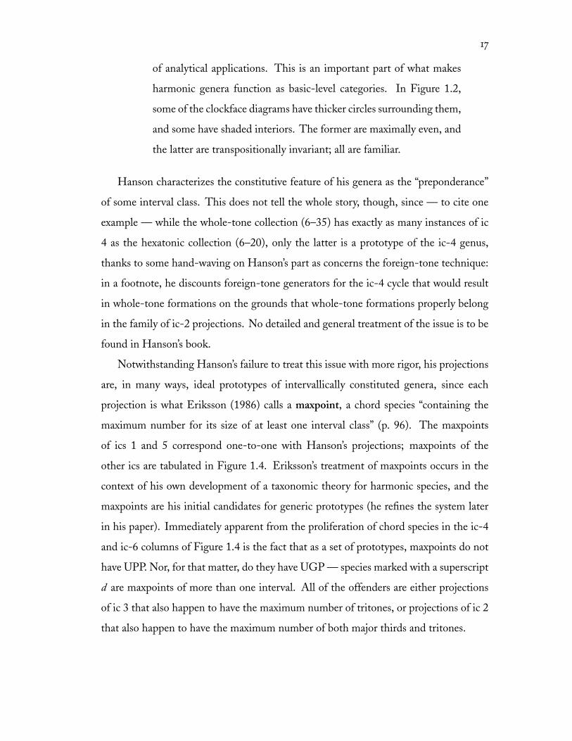
of analytical applications. This is an important part of what makes
harmonic genera function as basic-level categories. In Figure 1.2,
some of the clockface diagrams have thicker circles surrounding them,
and some have shaded interiors. The former are maximally even, and
the latter are transpositionally invariant; all are familiar.
Hanson characterizes the constitutive feature of his genera as the “preponderance”
of some interval class. This does not tell the whole story, though, since — to cite one
example — while the whole-tone collection (6–35) has exactly as many instances of ic
4 as the hexatonic collection (6–20), only the latter is a prototype of the ic-4 genus,
thanks to some hand-waving on Hanson’s part as concerns the foreign-tone technique:
in a footnote, he discounts foreign-tone generators for the ic-4 cycle that would result
in whole-tone formations on the grounds that whole-tone formations properly belong
in the family of ic-2 projections. No detailed and general treatment of the issue is to be
found in Hanson’s book.
Notwithstanding Hanson’s failure to treat this issue with more rigor, his projections
are, in many ways, ideal prototypes of intervallically constituted genera, since each
projection is what Eriksson (1986) calls a maxpoint, a chord species “containing the
maximum number for its size of at least one interval class” (p. 96). The maxpoints
of ics 1 and 5 correspond one-to-one with Hanson’s projections; maxpoints of the
other ics are tabulated in Figure 1.4. Eriksson’s treatment of maxpoints occurs in the
context of his own development of a taxonomic theory for harmonic species, and the
maxpoints are his initial candidates for generic prototypes (he refines the system later
in his paper). Immediately apparent from the proliferation of chord species in the ic-4
and ic-6 columns of Figure 1.4 is the fact that as a set of prototypes, maxpoints do not
have UPP. Nor, for that matter, do they have UGP — species marked with a superscript
d are maxpoints of more than one interval. All of the offenders are either projections
of ic 3 that also happen to have the maximum number of tritones, or projections of ic 2
that also happen to have the maximum number of both major thirds and tritones.
Page 28
18
card. ic 2 ic 3 ic 4 ic 62 2–2 [02]p 2–3 [03]p 2–4 [04]p 2–6 [06]p
3 3–6 [024]p 3–10 [036]pd 3–12 [048]p 3–5 [016]p
3–8 [026]3–10 [036]d
4 4–21 [0246]p 4–28 [0369]pd 4–19 [0148]p 4–9 [0167]p
4–24 [0248] 4–25 [0268]4–28 [0369]d
5 5–33 [02468]pd 5–31 [01369]pd 5–21 [01458]p 5–7 [01267]p
5–33 [02468]d 5–15 [01268]5–19 [01367]5–28 [02368]5–31 [01369]d
5–33 [02468]d
6 6–35 [02468A]pd 6–27 [013469]p 6–20 [014589]p 6–7 [012678]p
6–35 [02468A]d 6–30 [013679]6–35 [02468A]d
(p) indicates a maxpoint that is also a Hanson projection; (d ) indicates a “duplicate” maxpoint of several ics.
figure 1.4. Eriksson’s maxpoints.
One way to improve the situation would be to change the definition of a maxpoint.
Isolating certain special maxpoints (call them supermaxpoints) that not only maximize
some ic, but also have strictly more occurrences of that ic than any other chord species
of the same cardinality, reinstates a weak form of UPP. Rather than having multiple
prototypes of the same cardinality in certain genera, we now have no prototypes for
certain cardinalities in the genera associated with ics 4 and 6; otherwise the supermax-
points are coextensive with Hanson’s projections (see Figure 1.5). At the same time, this
maneuver solves the problem of UGP, since each of the multiply affiliated maxpoints
marked with a d in Figure 1.4 is a supermaxpoint of exactly one interval class. And, in
fact, the supermaxpoints are all also projections.
Noting problems akin to those that could be circumvented by isolating the su-
permaxpoints, and after an extensive discussion of abstract inclusion relations among
maxpoints (clearly related to IIP), Eriksson eventually abandons the idea of using chord
species as prototypes at all. Rather, his “model” for each of his seven genera (he calls
Page 29
19
card. ic 1 ic 2 ic 3 ic 4 ic 5 ic 62 2–1 [01]p 2–2 [02]p 2–3 [03]p 2–4 [04]p 2–5 [05]p 2–6 [06]p
3 3–1 [012]p 3–6 [024]p 3–10 [036]p 3–12 [048]p 3–9 [027]p
4 4–1 [0123]p 4–21 [0246]p 4–28 [0369]p 4–23 [0257]p
5 5–1 [01234]p 5–33 [02468]p 5–31 [01369]p 5–35 [02479]p
6 6–1 [012345]p 6–35 [02468A]p 6–27 [013469]p 6–32 [024579]p
figure 1.5. The “supermaxpoints.”
I II III IV V VI VII*typical ics 1 2, 4, 6 3, 6 4 5 6 2
↓ 21, 3, 5
21, 5 1, 5, 3, 4
3, 4 3, 4atypical ics 5, 6 1, 3, 5 1, 2, 4, 5 2, 6 1, 6 2, 3, 4 6
*Only M-invariant chord species may belong to this genus.
figure 1.6. Models of relative ic multiplicity in Eriksson’s seven “regions” (genera).
them regions) is a partial ordering of interval classes, ordered according to their fre-
quency of occurrence in a given species of chord. Figure 1.6, adapted from his Example
6, lists the models for the seven genera he eventually asserts. The highly suggestive
(and innovative) move from intervallic maxpoints to regional models is not without
problems — for example, the Petrushka chord 6–30 [013679] is a maxpoint of ic 6,
but its interval vector, 〈2, 2, 4, 0, 2, 3〉, resembles the genus III model of high ic-3 and
-6 content much more than it does the genus VI model, which specifically provides for
low ic-3 content.
1.2.2 Intrageneric affinities. In related work on a similarity-oriented theory, Michael
Buchler (2001) suggests that in order to compare two chord species on the basis of
their ic content, it is beneficial to contextualize the interval-class vector, as he puts it,
by means of “tools that take account of what is minimally and maximally possible in
a given cardinality” (p. 264), judging ic content relative to such possibilities. Buchler
calls the relativized measure of ic content the degree of saturation. A maxpoint for some
ic is, in Buchler’s terms, fully saturated with that ic. Setting aside for the moment the
considerations that lead Eriksson to supplement the theory of maxpoints with ic-vector
Page 30
20
“models” in asserting his generic prototypes, we observe that Buchler’s generalization
of maxpoints into degrees of saturation provides a fuzzification of the prototype idea.
A prototype is a very good example of a category; other members of a category may
be ranked in terms of their own goodness-of-example as well. We will use the term
intrageneric affinity to refer to this goodness-of-example relationship.
To the extent that interval content determines the intrageneric affinities of inter-
vallically constituted genera, one way to figure the affinity (degree of membership) of
a chord in such a genus might be to determine the degree to which the pcset-class is
saturated with the relevant ic (Buchler’s footnote 11 may be taken to suggest something
along these lines). Yet this sort of classification system would have as generic prototypes
all maxpoint pcsets, and thus inherit the UPP- and UGP-related problems discussed
above — the same problems that Hanson and Eriksson seek to avoid, each in his own
way. Recognizing this problem, Buchler defines what he calls the “maximal cyclic frag-
mentation condition” (p. 270), which is met by all and only the maxpoints singled out
as prototypes under Hanson’s system of projections (indeed, Buchler’s condition is pre-
cisely that used implicitly by Hanson). Buchler’s work is the background for a similarity
relation, though, and not a classification scheme, and he does not offer any suggestions
as to how one might go about fuzzifying the “maximal cyclic fragmentation condition”
in a way that would model intrageneric affinities for a system of genera constituted by
this specialized notion of interval-class saturation. For that matter, neither Hanson
nor Eriksson makes any finer distinction between members of a genus than between
prototypes and nonprototypes.
If the intrageneric affinities of a genus are the degrees to which various chord
species exemplify the genus, and if the best examples of a genus are its prototypes, then
a natural way to measure them with extant tools of pcset theory — and to provide the
“finer distinctions” we do not get from Buchler, Hanson, or Erikkson — is to consider
the similarity of a chord to generic prototypes using fuzzy similarity relations that are
based on interval content, such as Morris’s SIM and ASIM relations (1979), Isaac-
son’s IcVSIM (1990) and his various ISIMn relations (1996), and Scott and Isaacson’s
Page 31
21
ANGLE (1998). Scott and Isaacson provide a technical overview of the mathematical
connections among these relations, but all essentially measure the degree to which two
ic vectors have the same profile — in stark contrast to the “original” similarity relations
from Forte (1973), which neither come in degrees nor treat the ic vector as the sort
of thing that can have a shape, instead focusing on the yes-or-no question of whether
corresponding entries in two ic vectors are equal.
Fuzzy similarity relations do not directly suggest a system of prototypes, although
they do suggest genera (see Quinn, 2001). The discussions we have undertaken so far,
in connection with the intensional characterization of the aforementioned similarity
relations as being oriented toward interval content, suggest that Hanson’s system of
prototypes, or something like it, could form the basis of a generic taxonomy, with
similarity relations predicting (or modeling, if you prefer) the intrageneric affinities of
the genera. A more purely extensional approach might derive from the technique of
multidimensional scaling, which treats dissimilarity measurements among objects as
distances in a multidimensional space, then finds a distribution of the objects in the
space that provides a good fit with the data. Highly dissimilar objects will be far apart,
and highly similar objects will be close together. The application of multidimensional
scaling to data from chordal similarity relations tends to produce distributions in which
certain chords are at the “edges” of the distribution — thereby being as far away from
one another as possible — and these chords tend to be the prototypes we have been
discussing. Cognitively oriented work on multidimensional scaling of chord similarity
data has been conducted by Mavromatis and Williamson (1999), Samplaski (2000),
and Kuusi (2001).
Another approach might proceed from Eriksson’s prototypical models of ic-vector
shape. Block and Douthett (1994), who do not cite Eriksson’s article, present a related,
but more general approach (see, e.g., p. 22: “a composer may wish to find a family of sets
that have certain intervals suppressed or eliminated and at the same time have others
emphasized”). They develop a general structure (a “weight vector”) that corresponds
to such situations, and a procedure derived from vector algebra for determining how
Page 32
22
well a particular ic vector exemplifies this weighting. Many of the examples in their
article consist of a table of chord species arranged according to goodness-of-example,
and although they do not take the step of isolating prototypical ic-vector shapes —
this was Eriksson’s major achievement — it is the case that the ten such examples they
adduce are headed up by chord species corresponding to Hanson’s projections.
While any particular instance of these two approaches will likely produce similar
taxonomies (see Quinn, 2001), such an ad-hoc model would have pragmatic rather
than explanatory value, and not much pragmatic value at that: it would be useful for
answering questions that only straw men are asking (“how well is genus g exemplified
by species s?”) without shedding any light on interesting, abstract questions about why
so many superficially different theories converge at the basic level of chord quality. If
we seek more interesting questions, rather than answers to less interesting ones, we
should be highly suspicious of any such ad-hoc approach to answering questions about
intrageneric affinities.
Without committing to any particular approach yet, we will use the term Q-space
to describe an idealized spatial distribution of chord species, especially one that reflects
the intrageneric affinities of the qualitative genera we have been describing. (The term
reflects a scheme for naming qualitative genera with labels such as Q(12, 1), used in
Figure 1.2 and explained in § 2.3, infra.) The prototypes of each qualitative genus lie
in a particular “population center” of Q-space, and the spatial position of an arbitrary
chords reflects, by its distance from these various remote regions, its affinity to each of
the qualitative genera. Our ultimate goal is a theory of chord quality that describes Q-
space more specifically, and that makes the prediction that multidimensional scaling of
data generated by any of the particular procedures described above will produce spatial
distributions that converge on Q-space.
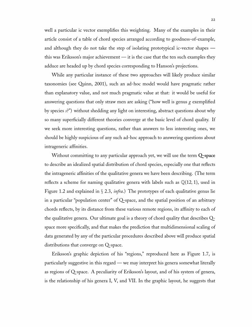
Eriksson’s graphic depiction of his “regions,” reproduced here as Figure 1.7, is
particularly suggestive in this regard — we may interpret his genera somewhat literally
as regions of Q-space. A peculiarity of Eriksson’s layout, and of his system of genera,
is the relationship of his genera I, V, and VII. In the graphic layout, he suggests that
Page 33
23
figure 1.7. Eriksson’s graphic representation of his genera.
VII is constituted by the overlap of peripheral parts of I and V; and in his description of
the intervallic model of genus VII he includes the caveat that such chord species must
contain equal numbers of ic 1 and ic 5, which is tantamount to asserting that they must
be invariant under M, the circle-of-fifths transform. These points, which we will revisit
a bit later (§ 1.3.2), throw into question the status of his genus VII as an independent
“population center,” since he seems to characterize it more as disputed territory between
the regions of genera I and V. Under this reading, we are left with (more or less) the
usual six intervallically constituted genera.
1.2.3 Intergeneric affinities. We have been imagining a fuzzy taxonomy for chord
species in which there are six genera roughly corresponding to the six interval classes.
Each genus is endowed with a structure described by its intrageneric affinities, which
depend on the notion of generic prototypes (best examples of genera) and the the idea
that the similarity of an arbitrary chord to the prototypes of a genus is equivalent to
the goodness-of-example of the chord to the genus. We now consider the question of
Page 34
24
how genera are related to one another, or how one might go about drawing analogies
between genera. Our case study will involve the genera associated with ics 1 and 5.
Two basic observations will get us going. First: any prototype of one of these two
genera, when subjected to the M5 (circle-of-fourths) or M7 (circle-of-fifths) transforms,
yields a prototype of the other genus; this is the case irrespective of whether one chooses
Hanson’s projections, Eriksson’s maxpoints or ic-vector models, our supermaxpoints,
or Buchler’s saturated chords to serve as prototypes. Second: suppose we have two
chords, and their degree of similarity is s (as measured by any of the similarity relations
mentioned above); transform both chords by M (by which we mean “either M5 or
M7”), and the degree of similarity between the transformed chords is also s. Choosing
an example at random, let p be an examplar of the species 4–27 [0258], and let q be
an exemplar of the species 6–13 [013467]. Buchler’s SATSIM reports their degree of
similarity as 0.261, and Scott and Isaacson’s ANGLE gives 0.117. Transforming p by
M yields an exemplar of 4–12 [0236]; q becomes an exemplar of 6–50 [014679] under
either transformation. Asked about the similarity of these latter two chords, SATSIM
gives 0.261 again, and ANGLE gives 0.117 again.
We will not attempt to prove here why intervallically constituted similarity relations
behave in this way (see Morris, 2001, ch. 4), but only to show that the two observations
just made allow us to make an interesting analogy between the two genera in question.
Since the intrageneric affinities of the genera are deterimined by similarity relations
involving their respective prototypes, and since the prototypes of the two genera are
swapped under certain transformations, and since the similarity relations determining
intrageneric affinities seem to be invariant under those same transformations, we can
draw the following general conclusion about the relationship among these two genera:
The degree to which a species (e.g., 6–3 [012356]) exemplifies one genus is the same
as the degree to which its M5-transform (e.g., 6–25 [013568]) exemplifies the other
genus. This conclusion pertains to what we will call the intergeneric affinities between
the two genera in question.
Page 35
25
M5c 0 5 A 3 8 1 6 B 4 9 2 7c 0 1 2 3 4 5 6 7 8 9 A B
“M2c” 0 2 4 6 8 A 0 2 4 6 8 A
figure 1.8. Multiplication by 2 as an epimorphism.
In a sense, this use of the word affinities is closely allied to the eponymous doctrine
of medieval theory, which concerns the relationship of different, but functionally iden-
tical, notes in different tetrachords. Each tetrachord has notes called protus, deuterus,
tritus, and tetrardus; these qualitative labels (intragenerically) describe the positions of
those particular notes in, say, the graves tetrachord. Affinities among the tetrachords
are described (intergenerically) by identity among the qualitative names and related,
coincidentally, by transpositions through fourths or fifths — the protus of the graves
tetrachord has an affinity to the protus of the finales tetrachord a fourth higher, and to
the protus of the superiores tetrachord a fifth above that.
The existence of intergeneric affinities between the two genera we have studied raises
the more general issue of affinities between any two genera. The M5 and M7 operators
relate the genera in question because each “expands” members of ic 1 into members of
ic 5, and further expands members of ic 5 into members of ic 1, all the while leaving all
other intervals invariant (up to interval-class). To generalize this to other genera, we
might briefly consider a multiplicative operator that expands members of ic 1 into other
intervals, but here we face Hanson’s original problem: the interval cycle. Suppose, for
example, we invent an operator that transforms every pc c into 2c (mod 12). Figure 1.8
contrasts this “M2” operator with the usual M5 operator; the problem is that while M5
and M7 (like the usual transposition and inversion operators) are one-to-one mappings
of the pitch-class universe onto itself, this “M2” is a many-to-one mapping. Any two
pcs separated by a tritone map to the same pc under “M2,” and no pcs map to an odd
pc under this operator.
In an unpublished manuscript (2000), Daniel Harrison notes this problem — which
is endemic to the generalization of multiplicative operators in the twelve-pc universe
— and presents a suggestive workaround. His N operator, which is a replacement for
Page 36
26
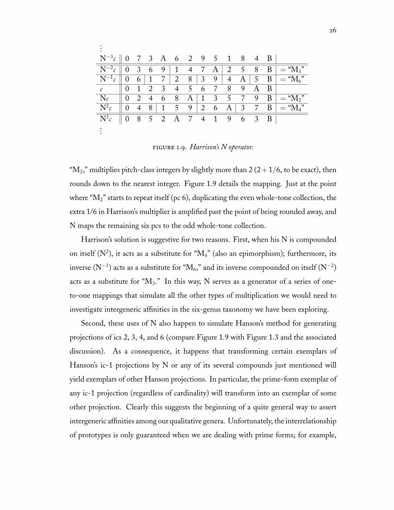
...N−3c 0 7 3 A 6 2 9 5 1 8 4 BN−2c 0 3 6 9 1 4 7 A 2 5 8 B = “M3”N−1c 0 6 1 7 2 8 3 9 4 A 5 B = “M6”c 0 1 2 3 4 5 6 7 8 9 A BNc 0 2 4 6 8 A 1 3 5 7 9 B = “M2”N2c 0 4 8 1 5 9 2 6 A 3 7 B = “M4”N3c 0 8 5 2 A 7 4 1 9 6 3 B...
figure 1.9. Harrison’s N operator.
“M2,” multiplies pitch-class integers by slightly more than 2 (2+1/6, to be exact), then
rounds down to the nearest integer. Figure 1.9 details the mapping. Just at the point
where “M2” starts to repeat itself (pc 6), duplicating the even whole-tone collection, the
extra 1/6 in Harrison’s multiplier is amplified past the point of being rounded away, and
N maps the remaining six pcs to the odd whole-tone collection.
Harrison’s solution is suggestive for two reasons. First, when his N is compounded
on itself (N2), it acts as a substitute for “M4” (also an epimorphism); furthermore, its
inverse (N−1) acts as a substitute for “M6,” and its inverse compounded on itself (N−2)
acts as a substitute for “M3.” In this way, N serves as a generator of a series of one-
to-one mappings that simulate all the other types of multiplication we would need to
investigate intergeneric affinities in the six-genus taxonomy we have been exploring.
Second, these uses of N also happen to simulate Hanson’s method for generating
projections of ics 2, 3, 4, and 6 (compare Figure 1.9 with Figure 1.3 and the associated
discussion). As a consequence, it happens that transforming certain exemplars of
Hanson’s ic-1 projections by N or any of its several compounds just mentioned will
yield exemplars of other Hanson projections. In particular, the prime-form exemplar of
any ic-1 projection (regardless of cardinality) will transform into an exemplar of some
other projection. Clearly this suggests the beginning of a quite general way to assert
intergeneric affinities among our qualitative genera. Unfortunately, the interrelationship
of prototypes is only guaranteed when we are dealing with prime forms; for example,
Page 37
27
N transforms {01234}, an ic-1 projection, into {02468}, an ic-2 projection; but it also
transforms {45678}, another ic-1 projection, into {1358A} — which is not only not an
ic-2 projection, but is also an ic-5 projection! The mathematical issue at hand is outside
the scope of our present inquiry, but the upshot is that any chord can be transformed
into any other chord of the same cardinality by some combination of N with the usual
transposition and inversion operators.
While N gets us tantalizingly close to a theory of intergeneric affinities, its explo-
sive interaction with the operators that define chord species tightly circumscribe its
usefulness. We will revisit the issue of intergeneric affinities in the next section.
§ 1.3 Other approaches to chord quality.
In addition to the intervallic approaches we have studied, theorists have explored
other ways of qualitatively relating chords. As we will see, much of the ground we
have covered so far is intimately connected to these other approaches, despite superficial
differences.
1.3.1 The inclusional approach. The most widespread alternative approach to chord
quality involves the ways in which chords include one another and, by extension, in
which chord species abstractly include one another. The large folding chart supplied by
Hanson (1960) details abstract inclusion relations among species in a manner that clearly
and vividly shows that chords tend to belong to the same genera as their subsets and
supersets. Nowhere in his book, however, does Hanson explicitly make this observation,
although his general approach (which involves extending the idea of projection from
intervals to trichords) is so thoroughly shot through with the idea of inclusion that,
to misuse Hanson’s own words (p. 272), one “may well ask whether any such detailed
analysis went on in the mind of the composer as he was writing the passage. The answer
is probably, ‘consciously—no, subconsciously—yes’.”
Page 38
28
Forte’s treatment of set complexes of the K and Kh types (1973) represent the first
explicit and thoroughgoing study of abstract inclusion relations that has a qualitative
character. It is useless as a generic taxonomic system, however, because if a pcset-
complex is a genus whose nexus is its prototype, it follows that any chord species
whatsoever can be a prototype of some genus. Forte’s nested complexes, however, show
an interesting parallel with the fuzzy generic structures we have been imagining. Each
K-complex, as a category, has a single prototype up to complementation; yet we may
interpret the Kh-subcomplex about that same prototype as a class of privileged members
of the K-complex — better examples of the genus. In Forte’s words, the idea of the
Kh-subcomples is to supply “additional refinement of the set-complex concept in order
to provide significant distinctions among compositional sets.”
Much later, Forte (1988) used similar principles to develop a quasi-taxonomic
system of what he calls genera and supragenera. There is still considerable overlap
among categories at the generic and suprageneric levels, but taxonomic hierarchicy
is more clearly manifest in this theory, since the supragenera wholly include their
respective genera. (At the same time, the number of chord species assigned to just
one genus, or even just one supragenus, is disappointingly small, and Forte offers no
further means of grading goodness-of-example within either level.) Introducing the
system, Forte announces that “we posit the intervallic content of pitch-class sets as the
fundamental basis of the genera” (p. 188), although this basis is operative only as far as
selecting generic prototypes (which are all trichords) is concerned, and from there the
constitutive principle is once again inclusion. Complicating the situation somewhat is
the fact that, strictly speaking, not all of his prototypes are trichords — some are pairs
of trichords that have two out of three ics in common. (For more on the relationship
between Forte’s genera and his set-complexes, see Morris, 1997.)
The conceptual bridge between thinking about interval content and thinking about
abstract inclusion relations was first solidly erected by Lewin (1977), who, observing that
an interval-class is simply a species of two-note chord, suggested that the qualitative
utility of thinking about interval content might be extended to the consideration of
Page 39
29
subset content generally. Not long thereafter, responding both to Morris’s development
of the first graded similarity relation, the ic-based SIM, and to Rahn’s subset-based
TMEMB, Lewin positioned his own REL as a conceptual generalization of both
(Morris, 1979; Rahn, 1980; Lewin, 1979).
Lewin’s observations, and other lines of thought that originate with them, may
help to explain why the interval-based approach to chord quality converges with the
subset-based approaches. On the one hand, similarity relations such as TMEMB and
REL that (more or less) simply count common subsets, as well as relations like Castren’s
fantastically complicated RECREL (1994), which compares the subset structures of
chord species rather than just the subsets, produce results that fall in line with those
produced by ic-based similarity relations when glimpsed from an extensional, taxonomic
point of view (Quinn, 2001). On the other hand, while the prototypes of Forte’s system
of genera are technically trichords or pairs of trichords, he frequently describes the genera
in “very informal descriptive terms so that the genera might seem more accessible and
familiar to the reader” (Forte, 1988, p. 200). These terms include whole-tone, diminished,
augmented, chroma[tic], and dia[tonic], which vividly recall the sorts of prototypes that
arise under strictly intervallic approaches. In the related generic system of Parks (1989),
similarly “accessible and familiar” terms arise. They are “informal” only because none
of the builders of formal chord-quality models seems to have been willing to take them
seriously enough to seek the appropriate formalizations instead of offering appeals to
intuition, which seem rather vacuous in the otherwise highly rigorous context of pcset
theory.
There are three good reasons to take these accessible labels seriously. The first has to
do with prototypes — the prototypes of a qualitative taxonomy constituted by inclusion
relations would seem to be precisely the same as those that fall out of an intervallic
approach. In particular, we have observed that Hanson’s prototypes have IIP and PCP,
which amounts to saying that the prototypes of any qualitative genus are Kh-related
to each other. We have also observed that they have PFP, which establishes a strong
Page 40
30
conceptual connection to Forte’s and Parks’s “accessible and familiar” names for their
own genera.
The second concerns intrageneric affinities, the modeling of which we have been
delegating to fuzzy similarity relations. It having been established that inclusional
similarity relations end up producing largely the same results as intervallic similarity
relations, there is good reason to suppose that they would agree as to the intrageneric
affinities of genera constituted by our working set of familiar intervallic-cum-inclusional
prototypes.
The third involves intergeneric affinities. We have yet to get terribly far with this
concept, but our observations concerning the M5 and M7 operations, which establish
affinities between Q(12, 1) and Q(12, 5) — now that we are no longer discussing interval
content per se, we will henceforth refer to qualitative genera by these symbols, which
were silently introduced in Figure 1.2 — carry over to the inclusional realm as well.
Suppose we have a chord p that includes a chord q; it follows immediately that M5p
includes M5q. From there it is a short journey to the conclusion that whatever an
inclusional similarity relation says about species s and t will be the same as what it says
about M5s and M5t, something that is borne out by all of the inclusional similarity
relations mentioned.
Most existing approaches to qualitative chord taxonomy belong to either the inter-
vallic or inclusional approaches. We have seen how these two types may be linked both
technically and conceptually, and how they tend to create similar sorts of genera. This,
perhaps, raises the question of which approach is “right.” On the face of it, this is rather
a silly question, which seems to invite intensional discourse of the sort I have argued
fervently against elsewhere. Hanson, for instance, says his projections are intervallically
conceived, but that does not disallow us from asserting, as we have, that they also have
a strong inclusional aspect, and that they seem to reflect maximal evenness and trans-
positional invariance in some way as well. At the same time, I am going to argue later
on that neither the intervallic nor the inclusional approach is “right,” and so I do not
wish to throw out the question as intensional and therefore trivial. Rather, the question
Page 41
31
should be viewed as theoretical and therefore explanatory in nature — the theory of
chord quality we are developing seems to transcend the distinction between intervallic
and inclusional approaches, largely because the intervallic and inclusional aspects of the
generic prototypes and affinities converge; neither is necessary or sufficient to explain
the other. Furthermore, there are a few loose ends concerning maximal evenness and
transpositional invariance (which seem to be contributing factors to the all-important
PFP), and considerably more loose ends concerning intergeneric affinities, that we are
as yet at a loss to explain.
Our survey will continue and conclude with a study of two sharply distinctive
approaches to the construction of genera that will take us away from the intervallic
and inclusional approches, and advance us toward an understanding of said loose ends.
These two approaches are truly sui generis, so to speak, in terms of both the constitution
of genera and the nature of the genera that are thereby constituted.
1.3.2 Morris’s algebraic approach. In the tradition of mainline pcset theory, Morris
(1982, 2001) adheres strictly to what Lakoff characterizes as the “classical view” of
categories — that the extension of a category is a set, and that the intension of a
category is a collection of necessary and sufficient conditions. Morris begins with a
survey of the common approaches to gathering chords into species, referring to each
such approach as a set-group system. He cites four, describing the intensional conditions
for species in each system; to paraphrase:
• Under SG(v), two chords belong to the same species if and only if they have the
same interval content.
• Under SG(1), two chords belong to the same species if and only if they can be
transformed into one another by pc transposition.
• Under SG(2), two chords belong to the same species if and only if they can be
transformed into one another by pc transposition and/or pc inversion.
Page 42
32
• Under SG(3), two chords belong to the same species if and only if they can be
transformed into one another by pc transposition and/or pc inversion and/or the
circle-of-fifths transform M .
Morris uses the term set-group in a highly general sense; because he does not assert
anything like a basic level of classification, there is no way to make a distinction of
kind between species and genera. Yet the taxonomic instinct looms large in his theory
of set-group systems. Much of this theory is concerned with the ways in which one
set-group system can be hierarchically related to another, in the hard-and-fast manner
of Linnaean species, genera, familiæ, ordines, and so forth up the taxonomic ranks.
Generalizing Lakoff ’s terminology, we might assert a classical view of taxonomy that
can be characterized inductively: each taxonomic rank is a classical system of categories,
and any two things classified in the same category at a given rank are necessarily classified
in the same category at all higher (coarser) ranks. Morris’s discussion of the four set-
group systems just listed strongly implies a classical view of taxonomy; much of his initial
discussion amounts to the observation that SG(1), SG(2), and SG(3) may be successive
ranks of a classical taxonomy. His subsequent development of an array of additional
set-group systems seems to be motivated by frustration that SG(v) cannot be worked
into a classical taxonomy with the other three. In particular, SG(v) is taxonomically
superior to both SG(1) and SG(2), but is taxonomically neither superior nor inferior
to SG(3). (Counterexamples are 5–12 [01356] and 5–36 [01247], which are not M-
related but do have the same interval content; and ics 1 and 5 themselves, which are
M-related but clearly do not have the same interval content.) Morris initially suggests
a bit of fudging: if we were to decree ic 1 and ic 5 to be identical, redefining “interval
content” accordingly, the problem would go away, with SG(v) taking its place in the
hierarchy just above SG(3).
Assuming that by “species” we mean the taxa of SG(2), which are the just the familiar
pcset-classes of Forte (1973), we may choose either SG(3) or any of its superior set-group
systems to function as what we have been uniformly calling genera. For reasons that
will be immediately evident, let us distinguish between the algebraic genera of Morris’s
Page 43
33
ic-1 genus ic-5 genusprototype 5–1 [01234] 5–35 [02479]
↓ 5–2 [01235] 5–23 [02357]↓ 5–3 [01245] 5–27 [01358]↓ 5–9 [01246] 5–24 [01357]
distant 5–33 [02468] 5–33 [02468]
figure 1.10. Morris’s algebraic SG(3) genera (rows) versus qualitative genera (columns).
set-group taxonomy and the qualitative genera that have been our main topic thus far.
Even with SG(3) itself, we see something completely different happening in Morris’s
taxonomy than with all of the other approaches we have discussed to this point. Recall
that all of those systems (implicitly or explicitly) include separate qualitative genera for
ic 1–type and ic 5–type chord species, the prototypes of which are connected segments
of the chromatic scale and the circle of fifths, respectively; then note that by assigning
M-related chord species to the same algebraic genus, the SG(3) system asserts algebraic-
generic equivalence between pairs of qualitative prototypes. Any Q(12, 1) prototype is
the M-transform of the Q(12, 5) prototype of the same cardinality, and vice versa.
Consider now the chord species displayed in Figure 1.10. They are arranged into
two columns that correspond to the fuzzy qualitative genera Q(12, 1) and Q(12, 5),
respectively. The top row contains prototypes of each genus, and successively lower
rows contain species more distant from the prototypes (most similarity relations will
agree on this). At the same time, the two entries in each row are M-related to one
another, and consequently belong to the same “genus” of SG(3). What this means is
that SG(3) brings together species that play the same role in two different qualitative
genera that are wholly M-related to one another.
What we are dealing with, of course, is the the same phenomenon we discussed
earlier in connection with intergeneric affinities between the qualitative genera. Two
chords belong to the same algebraic genus of SG(3) if and only if there is an intergeneric
affinity between them with respect to the two qualitative genera in question. In this
sense, Morris’s algebraic genera are exactly orthogonal to qualitative genera — and in a
way that engages an important feature of the system of qualitative genera.
Page 44
34
5–33 [02468]
5–9 [01246]
5–3 [01245]
5–2 [01235]
5–1 [01234]
5–24 [01357]
5–27 [01358]
5–23 [02357]
5–35 [02479]
M
M
M
M
II
I V
figure 1.11. M5 structures certain intergeneric affinities; it also preserves certain intragenericaffinities.
Referring back to Eriksson’s map of his genera (Figure 1.7), and pretending that this
is in fact a map of Q-space, let us locate the chord species of Figure 1.10 on the map.
The locations of the prototypes 5–1 [01234] and 5–35 [02479] are where Eriksson
has marked “I” and “V,” respectively. The species 5-33 [02468], in the bottom row
of Figure 1.10, is a prototype of the qualitative genus Q(12, 6), which, because of that
genus’s association with ic 2, can therefore be located where Eriksson has marked “II.”
Now draw two straight lines from 5–33: one to each of the two prototypes 5–1 and
5–35. Distribute the other chord species from the two columns of Figure 1.10 evenly
along those two lines, and in the same order. The resulting distances are very roughly
those that most similarity relations will estimate for all of the chord species involved.
The arrangement just described, and sketched in Figure 1.11, is consistent with the
following assertion: The M operation corresponds to a reflection (flip) about a vertical
line running through the center of Figure 1.7. This assertion, in turn, is consistent
with two important observations. First, as we have already noted, Eriksson’s genus VII
consists, by fiat, entirely of M-invariant chord species. In his graphic representation,
that genus lies between I and V and directly on the axis of reflection corresponding to
M. Second, as we have not previously noted, nearly all of the agreed-upon prototypes
of the genera associated with ics 2, 3, 4, and 6 are M-invariant. Again, in Eriksson’s
graphic representation, the centers of these genera lie directly on the axis of symmetry in
Page 45
35
question. (Oddly, Eriksson does not discuss the circle-of-fifths transform at all, despite
the fact that many of his figures display this vivid symmetry.)
We have been emphasizing for some time that M5 structures intergeneric affinities
between Q(12, 1) and Q(12, 5), but have just noted that the prototype of the other four
genera are all invariant under M5. Recall now from our initial discussion of intergeneric
affinities that the similarity of two chords p and q is exactly the same as the similarity of
M5p and M5q. Suppose that p is invariant under M5; then it follows that q and M5q are
each identically similar to p — which leads us immediately to the conclusion that that
M5 preserves the intrageneric affinities of these other four genera. Thus Figure 1.11
may be taken as a demonstration not only of M5’s role in structuring the intergeneric
affinities between Q(12, 1) and Q(12, 5), but also of the invariance of the intrageneric
affinities of Q(12, 6) under M5.
The algebraic genera of SG(3) — or, more particularly, the taxonomic relationships
between SG(2) and SG(3) — engage all of the issues raised by qualitative genera, but
from an orthogonal point of view. That being the case, we should be particularly
interested in Morris’s major question: What would SG(4) be? Each of the numbered
set-group systems relates to its taxonomically inferior rank by adding to the canon of
equivalence operators. Therefore such an SG(4) could be created by finding some other
permutation of pcs (in addition to transposition, inversion, and M) and elevating it to
the status of an equivalence operator. In particular, Morris is interested in operators
that
preserve certain interval-classes while changing others in the pcsets they
transform. In this way the vectors of the mapped sets will be able to
retain some of their features. As a result, the set-groups within the set-
groups systems we will develop will be related by a kind of similarity
measure. Fortunately, all of these strictures are inter-related; by actualizing
one property we will gain the others (1982, pp. 113–13).
Such nonstandard operators will only be useful if they do not simply collapse all chords
of a single cardinality into one category — Harrison’s N operator does this, since, as
Page 46
36
discussed above, it can be used in combination with transposition and inversion to turn
any chord into any other chord of the same cardinality.
Each of Morris’s nonstandard operators begins with a partition of the aggregate into
identical dyads, then maps each pc in each dyad into the other. For his α, for instance,
he partitions the aggregate into six instances of ic 1. There is only one way to do this
(up to transposition):
{0,1}{2,3}{4,5}{6,7}{8,9}{A,B}.
Note that in this partition, the ic-1 dyads are arranged along an “outer” ic-2 cycle. The
α operator simply swaps the pcs within each of these dyads; another way to describe
this is that each pc in the even whole-tone collection gets transposed up a semitone, and
each pc in the odd whole-tone collection down a semitone. Immediately we can see
that every prototype species of Q(12, 6) is necessarily invariant under α; it happens that
the prototypes of Q(12, 3) are also invariant. One would do well to wonder whether
these invariances generalize from the particular prototypes of these genera to their
intrageneric affinities as a whole, as we saw to be the case with M5’s preservation of the
intrageneric affinities of four qualitative genera.
The α operator does not leave any other generic prototypes invariant, but it does
something suggestive to the prototypes of Q(12, 2) and Q(12, 4) — associated, respec-
tively, with ics 6 and 3. Consider the tetrachordal prototypes, which are 4–9 [0167] and
4–28 [0369]. Thanks to transpositional and inversional invariances, there are only six
exemplars of the former, and just three of the latter. All three of the 4–28 chords become
4–9 chords when transformed by α. Since α (like all of Morris’s nonstandard operators)
is its own inverse, those 4–9 chords — {1278}, {349A}, and {56B0} — transform into
exemplars of 4–28 under α as well. The other three 4–9 chords — {0167}, {2389}, and
{45AB} — are invariant under α. As a result, this pair of species constitutes a single
algebraic genus under SG(α). Indeed, the prototypes of these two genera invariably
relate to one another via α, with one exception: the hexachordal Q(12, 2) prototype, 6–7
Page 47
37
op. partition
genera with prototypes. . .
invariant swapped
α {0,1} {2,3} {4,5} {6,7} {8,9} {A,B} Q(12, 3) Q(12, 2), Q(12, 4)Q(12, 6)
β {0,2}, {1,3}, {4,6}, {5,7}, {8,A}, {9,B} Q(12, 3)γ {0,3}, {1,4}, {2,5}, {6,9}, {7,A}, {8,B} Q(12, 2)
{0,3}, {2,5}, {4,7}, {6,9}, {8,B}, {A,1} Q(12, 4)δ1 {0} {1} {2} {3} {4,8} {5,9} {6,A} {7,B} Q(12, 3) Q(12, 1), Q(12, 4), Q(12, 5)δ2 {0} {1} {2} {7} {B,3} {4,8} {5,9} {6,A} Q(12, 3)δ5 {0} {1} {3} {6} {A,2} {4,8} {5,9} {7,B} Q(12, 3) Q(12, 1), Q(12, 4), Q(12, 5)
figure 1.12. Morris’s nonstandard operators.
{012678}, is transformed by α not into Hanson’s hexachordal ic-3 projection, but into
the closely related Petrushka chord, 6–30 [013679]. (But remember that our elevation
of Hanson’s projections to prototype status is not infallible, and that 6–30 is a maxpoint
of ic 6, among other things.) The obvious question concerning affinities is whether α
describes intergeneric affinities between Q(12, 2) and Q(12, 4).
Without delving deeply into Morris’s theory, we observe that the other operators
are constructed likewise (beginning with other homogeneous partitions of the aggre-
gate), and produce similarly interesting results. The table in Figure 1.12 lists the six
nonstandard operators Morris uses to construct set-group systems. As α is based on a
partition into ic-1 dyads, β and γ stem from ic-2 and ic-3 partitions, respectively. The
aggregate cannot be partitioned into six discrete instances of ic 4, so Morris constructs a
family of δ operators based on best-case partitions, of which only three generate unique
set-group systems.
It should be observed that the intervals (and corresponding prototypes) preserved
under each operator are not necessarily the same as those involved in the partition
underlying each operator. We saw that the ic-1 partition underlying α is best understood
as being structured by an ic-2 cycle; thus it is the ic-2 and ic-4 prototypes that are
preserved. Similarly, the ic-2 partition underlying β is structured by a hexatonic scale,
a prototype of the genus Q(12, 3), all of whose prototypes are β-invariant. The two
possible ic-3 partitions (generating γ) are structured by 6–7 [012678], a prototype of
Q(12, 2), and the whole-tone collection, with appropriate invariances ensuing.
Page 48
38
Each one of the six nonstandard operators leaves some array of generic prototypes
invariant, raising the possibility of intrageneric-affinity preservation. Three (α, δ1,
and δ5) consistently conflate prototypes of different genera into the same set-groups,
raising the possibility of intergeneric affinities. (Since each operator is a “root” of M5,
each conflates prototypes of Q(12, 1) and Q(12, 5), which is not mentioned in the table.)
Insofar as we have had some general success in describing affinities in terms of prototypes
and similarity relations, the questions just raised about the relationship between Morris’s
set-group systems and the affinities of the qualitative genera are empirical ones. The
event is that the nonstandard operators do not, on the whole, work as neatly as we
might have hoped in the general case, despite their tidy treatment of the prototypes.
1.3.3 Cohn’s cyclic approach. As an adjunct to his theory of transpositional invariance,
Cohn (1991) develops five set-group systems of his own. Each is based on a special kind
of nonstandard multiplicative operator he calls a CYCLE homomorphism, q.v. also Starr
(1978). The “M2” operator we discussed above in connection with Harrison’s N operator
is one of these (CYCLE-6). Cohn is interested in taking advantage of precisely the
same characteristic of these operators that Harrison viewed as a problem — specifically,
that they do not necessarily preserve cardinality. A simple example, which we have
already considered, concerns the transformation of a tritone under CYCLE-6 (“M2”),
which becomes a single pc. From a certain point of view, there is something missing
from this statement — one might like to think that the CYCLE-6 transform of a tritone
is actually two “copies” of the same pc — but in the usual framework of pcset theory,
which treats chords as classical sets of pitch-classes, there is no technical facility for
making counting “copies” of a pc in a chord. Lewin (1977) and Morris (1998) have both
suggested that such a facility, sometimes known as a multiset, might come in handy in
certain theoretical contexts, but the important and fascinating issues involved constitute
a can of worms best left closed in the present context.
Figure 1.13 lists the five CYCLE homomorphisms, along with the multiplicative
operators they closely resemble. In Cohn’s conception, the homomorphisms “act not
Page 49
39
0 1 2 3 4 5 6 7 8 9 A B“M2” 0 2 4 6 8 A 0 2 4 6 8 A
CYCLE-6 0 1 2 3 4 5 0 1 2 3 4 5 (mod 6)“M3” 0 3 6 9 0 3 6 9 0 3 6 9
CYCLE-4 0 1 2 3 0 1 2 3 0 1 2 3 (mod 4)“M4” 0 4 8 0 4 8 0 4 8 0 4 8
CYCLE-3 0 1 2 0 1 2 0 1 2 0 1 2 (mod 3)“M6” 0 6 0 6 0 6 0 6 0 6 0 6
CYCLE-2 0 1 0 1 0 1 0 1 0 1 0 1 (mod 2)“M12” 0 0 0 0 0 0 0 0 0 0 0 0
CYCLE-{1,5} 0 0 0 0 0 0 0 0 0 0 0 0 (mod 1)
figure 1.13. Cohn’s CYCLE homomorphisms as multiplicative operators.
only upon individual pitch classes, but on all mod-12 pc sets as well, mapping them
into set classes within smaller universes.” These smaller universes are represented by
the integers modulo n, where n is the number of the CYCLE homomorphism. There is
an important, but subtle, shift of perspective contained in Cohn’s invocation of smaller
universes here; it is most clearly manifest in the mismatch between the numerical labels
of the “Mm” operators and their associated CYCLE-n homomorphisms.
Cohn captures this shift of perspective in a diagram adapted here as Figure 1.14. The
lighter circles in the diagram represent interval cycles; they also represent the collections
of pcs that map identically under the relevant CYCLE homomorphism. The heavier
circles represent what Cohn calls “cycles of cycles” (p. 12). This terminology refers
to the fact that the CYCLE homomorphisms involve collapsing interval cycles into a
representative indicated here with large type; this representative “may be thought of as
not only furnishing a label for that cycle, but as vortically inhaling its contents” (p. 14)
under the relevant homomorphism. Once the interval cycles are collapsed, it is clear
that the cycles are themselves cyclically related to each other; this accounts for the
periodic nature of the mappings detailed in Figure 1.13, clarified there with vertical
lines. The “cycles of cycles” are Cohn’s “smaller universes.”
In simple terms, this shift of perspective calls into question the usual interpreta-
tion of multiplicative operators and subjects them to a sort of figure-ground reversal
Page 50
40
4
5
7
2
3
8
9
A
B
0
6
1 45
7
3
8
9
AB
0
6
12
4
57
8
9
A
B
0
6
1
2
3
016
9
8
7B
A
23
4
5
CYCLE-2 CYCLE-6 CYCLE-3 CYCLE-4
figure 1.14. Adapted from Cohn (1991), Table 5.
— conceptualizing them not as things that expand intervals within the fixed frame
of octave equivalence, but as things that preserve intervals while shrinking the uni-
verse. Each of the CYCLE homomorphisms, as Cohn uses them, extends the idea
of octave equivalence to smaller intervals. CYCLE-2 envisions a world of whole-tone
equivalence; CYCLE-3, minor-third equivalence; CYCLE-4, major-third equivalence;
and CYCLE-6, tritone equivalence. Cohn’s set-groups are nothing more than chord
species of the usual kind — equivalence classes of classical sets of pitch-classes under
transposition and inversion — but under these novel notions of pitch-class equivalence.
Cohn gets to this point, as we have mentioned, through a study of transpositionally
invariant chords. Many of these are Hanson projections — all, in fact, besides the
French-sixth chord 4–25 [0268] and the Petrushka chord 6–30 [013679] — and are
therefore depicted in Figure 1.2, where the interior of their clockface diagrams are
colored gray. Inspection of these graphical representations highlight Cohn’s point: a
transpositionally invariant set exhibits a repeated pattern that is periodic at one of the
intervals of equivalence mentioned above. The hexatonic collection 6–20 [014589],
for instance, a prototype of what we are calling Q(12, 3), is periodic at the major
third. Since the pattern is periodic modulo 12, its structure can be completely, and
more efficiently, described in terms of a nonperiodic pattern in a smaller universe; the
mapping from the twelve-pc universe down to the smaller universe is provided by a
CYCLE homomorphism.
Page 51
41
We are now in a position to discuss the mismatch between our labels for the
qualitative genera and the labels for the interval-classes associated with them. This
is precisely the same as the mismatch noted above between the numerical labels of
the “Mm” operators and their associated CYCLE-n homomorphisms. The hexatonic
collection is periodic at the major third. This interval being a representative of ic 4, the
CYCLE-4 homomorphism provides the mapping into the requisite smaller universe
(major-third equivalence). When we characterize CYCLE-4 as “M3,” or when we assert
the species 6–20 as a prototype of the Q(12, 3) genus, we are making reference to the
fact that there are three major thirds to the octave. Similar statements could be made
about, for example, CYCLE-2, ic-2 equivalence, and the transpositionally invariant
whole-tone collection 6–35 [02468A], on the one hand, and “M6,” six whole-tones to
the octave, and 6–35 as a prototype of Q(12, 6) on the other. The clockface diagrams in
Figure 1.2 are each supplemented with markings that show their division into q equal
parts, where q is the index of the qualitative genus Q(12, n).
Cohn’s approach opens up a number of interesting avenues of inquiry in relation
to the issues that have been placed on the table so far. The various approaches we
have considered all seem to suggest, in one way or the other, that intergeneric affinities
(the structural relationships between qualitative genera) have something to do with
multiplication and interval cycles. Moreover, the prototypes laid out in Figure 1.2
— which, despite the fact that Hanson conceived them intervallically, have strongly
resonanted throughout our survey of different approaches to chord quality — seem to
warrant further inquiry from the point of view of transpositional invariance, given how
many of them have that symmetry. Cohn’s work appears to tie all of these ideas together,
suggesting that chord quality has something to do with equal divisions of the octave,
but it raises two important questions of its own.
First, there are five CYCLE homomorphisms and six qualitative genera. CYCLE-
{1,5}, which simply collapses all pcs into one category under semitone- or fifth-
equivalence, corresponds in some vague sense to Q(12, 1) and Q(12, 5), if only con-
ceptually, but these are precisely the genera whose only transpositionally invariant
Page 52
42
prototypes are trivial — the empty chord and the aggregate — and also in violation of
UGP, if trivially so. What the prototypes of these genera have in common is something
we have not yet treated adequately: each is a contiguous segment of the chromatic scale
in the case of Q(12, 1), or the circle of fifths in the case of Q(12, 5).
Second, the concept of a one-to-one mapping between interval classes and divisions
of the octave, which may be implied by the strong connection between Cohn’s approach
and our working set of prototypes derived from Hanson’s intervallic approach, is tenuous
at best. Our best example of this in the twelve-pc universe has to do with Q(12, 5) —
the octave is not equally divisible into 5 equal parts. Nonetheless, it is well-known that
certain of our prototypes for Q(12, 5), viz. the pentatonic collection 5–35 [02479] and
its complement, the diatonic collection), are maximally even; they represent the best way
to distribute five pcs (or five absences-of-pcs) equally around pitch-class space. As it
happens, these chords can also be generated by ic 5 — what may come as a disappointing
surprise, as we will see in the next chapter, is that this property does not generalize in
the obvious way (see Carey and Clampitt, 1996).
Having completed our survey of existing approaches to qualitative taxonomy, we
will change course now, pursuing the promising idea of equal divisions of a pitch-class
universe, which is covered by the theory of maximally even chord species. This will
be the key to fitting together some of the seemingly incompatible approaches we have
covered here.
Page 53
43
chapter 2
A unified theory of generic prototypes
Now that we have found common cause among all of the various approaches to chord
quality we have surveyed, and seen that they are rather tightly interrelated to one
another, the complexity of the theoretical task ahead should be clear. It seems that
three abstract concepts — prototypes, intrageneric affinities, and intergeneric affinities
— can provide the infrastructure of a theory of chord quality; our task is to make these
concepts concrete in the domain of chords and species.
Rather than starting from the bottom up, proceeding from any one of the approaches
covered in Chapter 1, we will take a top-down approach, wiping the slate clean and
taking as our point of departure a theoretical framework from scale theory (Clough and
Douthett, 1991), the original intent of which was to generalize certain aspects of the
diatonic scale. (In the broadest sense, that is our intent as well: the diatonic scale, after
all, is a generic prototype.) As we generalize Clough and Douthett’s work outward into a
theory of generic prototypes, we will find ourselves subsuming certain key notions from
each of the approaches that have been covered so far, fitting them into the emerging
unified framework. At times the work will, of necessity, be highly technical. The
business of Chapter 3 will be to develop an approach to affinities that interfaces with
this theory of prototypes; our treatment of that approach will retroactively clarify and
simplify much of the technical language that comes up below.
Page 54
44
§ 2.1 Maximally even subgenera.
Although it is assumed that the reader is familiar with Clough and Douthett’s
remarkable paper on maximally even chords and chord species, we will begin by sum-
marize and recasting some of their results, periodically adding some new terms concepts
into the mix. An asterisk (*) denotes a term or usage original to this work. Page and
theorem numbers in this section refer to Clough and Douthett’s paper unless otherwise
specified. Following Clough and Douthett’s usage, the variable c will stand for the
number of pcs in a given pitch-class universe; the variable d will generally stand for the
cardinality of a chord or species.
A maximally even (ME) chord is one “whose elements are distributed as evenly
as possible around the chromatic circle” (p. 96). There is at least one ME chord of
every cardinality in every chromatic universe (Theorem 1.2, p. 102). Any transposition
of a ME chord is also ME, and conversely, all ME chords of a given cardinality in a
given chromatic universe are related by transposition (Theorems 1.6 and 1.7, p. 108).
Furthermore, all ME chords are inversionally invariant (Theorem 1.8, p. 109).
The foregoing may be summarized by observing that all ME chords of the same
cardinality in the same chromatic universe belong to the same inversionally invariant
species, and, conversely, that all members of that species are ME. Let M(c, d) stand for
the unique ME species of cardinality d in a universe of c pcs. A ME chord is a singleton
if d = 1, an antisingleton* if d = c − 1, and trivial if d = 0 or d = c. Singletons and
antisingletons (and various equivalence classes of them) are semitrivial* (but not trivial).
We recall that the abstract complement of a ME species is also ME (Theorem
3.3, p. 150; Corollary 3.2, p. 151). The chords in a ME species, together with their
complements, constitute a ME subgenus*. Let M(c, d) stand for the ME subgenus
including M(c, d) and its complement.
The number of ME subgenera in a c-pc universe is equal to c/2 rounded down to the
nearest integer. (This is the same as the number of interval classes in the universe.) As a
preview of what is to come, our theory of chord quality will entail making a one-to-one
Page 55
45
correspondence between nontrivial ME subgenera and qualitative genera; a sense of this
can be had by inspecting Figure 1.2 (in which ME species are indicated with thicker
circles) and considering the relationship between the species of M(c, d) and the other
prototypes of Q(c, d).
A stern warning is in order at this point: although in any pitch-class universe, the
number of ME subgenera is equal to the number of interval classes, there is no natural
and general way to draw a one-to-one correspondence between them. We issue the
warning because it happens to be possible to do so in the usual 12-pc universe, which
leads to the fallacious notion that the interval content of a chord is a cause (and not a
symptom) of its qualitative relationship to other chords. From time to time we will refer
to this notion as the Intervallic Half-Truth. To understand the Intervallic Half-Truth
in sufficient depth, we need to pursue the question of how interval classes become
associated with ME chords in the first place. This will require a small amount of new
work relating to the classification of ME species.
It is established above that M(c, d) exists for any c and d , and that its exemplars are
inversionally invariant. Clough and Douthett show that, M(c, d) will have at least one
of the following two additional properties, depending on the greatest common factor of
c and d :
(TINV) If and only if gcf(c, d) > 1, exemplars of M(c, d) are nontrivially
transpositionally invariant, and the index*, or number of distinct
exemplars, of M(c, d) is given by c/gcf(c, d). (Theorem 1.9, p. 113)
(G) If and only if gcf(c, d) = 1 or gcf(c, d) = d , M(c, d) is generated
(Theorem 3.1, p. 148). That is, for any exemplar, there is at least one
way of ordering the constituent pcs (up to reversal) such that any two
adjacent pcs are separated by the same interval — as, for instance,
one can order a diatonic collection as a contiguous segment of the
circle of fourths/fifths. Such an ordering will be called a generated
ordering; the interval between adjacent pcs of a generated ordering is
Page 56
46
the generating interval and the interval between the last and first pcs
of a generated ordering is the wraparound interval.
We will use these properties, in conjunction with the theory of complementation,
as the basis of a fourfold classification of ME species that is related to Clough and
Douthett’s threefold classification (p. 148), but slightly stricter and more germane to
our overarching theoretical goals.
In a later article, Clough et al. (1999, Theorem 3.2, pp. 91–93) prove that all ME
species that are G are also well-formed (WF) in the sense of Carey and Clampitt
(1989), meaning that each instance of the generating interval spans the same number
of scale steps — e.g., the generating fifths of a diatonic collection span five scale steps,
which is why they are called fifths. We mention this in order to take advantage of
the latter’s distinction between what they call degenerate and nondegenerate WF species,
which distinction features prominently in the former’s proof. All WF species (ME or
not) are G. Degenerate WF species have the property that in any generated ordering,
the generating interval is equal to the wraparound interval, guaranteeing that they will
be TINV; nondegenerate WF species have the property that in any generated ordering,
the generating interval is not equal to the wraparound interval, guaranteeing that they
will not be TINV. There is no third option; every WF species is either degenerate or
nondegenerate. Here is how the distinction carries over to ME species:
Class I If and only if c and d are coprime (i.e., gcf(c, d) = 1), then M(c, d)
is G and nondegenerate WF. Because c is not evenly divisible by d ,
it is ME only in the sense that its constituent pcs are “distributed
as evenly as possible around the chromatic circle.” The fact that ev-
ery possible generating interval is different from the corresponding
wraparound interval precludes the possibility that M(c, d) is TINV.
In the event that M(c, d) is semitrivial (that it is a singleton or anti-
singleton) it is certain that gcf(c, d) = 1, and that the nondegenerate
status claimed for M(c, d) is, since the existence of generating and
wraparound intervals is somewhate questionably, strictly by fiat.
Page 57
47
Class IIa If and only if d divides c (i.e., gcf(c, d) = d) and d > 1, then
M(c, d) is G and degenerate WF. Because d divides c evenly, its
constituent pcs are distributed perfectly evenly around pitch-class
space, in contrast to a Class I species. M(c, d) is therefore TINV.
In the usual pitch-class universe, the ME species of Class I (G and TINV) are either
singletons or antisingletons, or pentatonic collections or their complements (diatonic
collections). The ME species of Class IIa (G and not TINV) are tritones, augmented
triads, diminished-seventh chords, or whole-tone collections.
Having exhausted the cases in which ME species are G, our classification of ME
species will be completed by cases that are TINV but not G. These we will divide into
two types distinguished primarily by their behavior under complementation. We have
already mentioned that the complement of any ME chord is itself ME; consequently
any species M(c, d) is the abstract complement of M(c, c − d). An elementary theorem
of number theory holds that gcf(c, d) = gcf(c, c − d). It follows that the (abstract)
complement of a Class I species is the complement of another Class I species, since in
that case gcf(c, d) = gcf(c, c − d) = 1.
Suppose M(c, d) is not G; then 1 < gcf(c, d) < d (Theorem 3.1, p. 148) and M(c, d)
is TINV (Theorem 1.9, p. 113–14). All such species can be divided into two types:
Class IIb If and only if 1 < gcf(c, d) < d and gcf(c, d) = c − d , then
M(c, d) is the complement of a Class IIa species, and we say that it is
complement-generated* (CG), which means simply that its comple-
ment is generated. Note that the complement of a Class IIa species
is of Class IIb if and only if d is not exactly half of c, as is the case
with the usual whole-tone collections (Theorem 3.4, p. 151–52). In
such cases the complement of a Class IIa species is “another Class
IIa species” in a somewhat trivial sense. Diverging from Clough and
Douthett’s practice, we will allow for purposes of argument that all
CG species have generating intervals — the same as that of their gen-
erated complements — even though they are not generated, strictly
Page 58
48
class definition g? cg? tinv? compl.
I gcf(c, d) = 1 yes yes no IIIa gcf(c, d) = d 6= 1 yes no yes IIb*IIb gcf(c, d) = c − d 6= 1 no yes yes IIaIII otherwise no no yes III
*Unless c = d/2, in which case Mc,d is its own complement (up to transposition).
figure 2.1. Classification of all ME species for c > 1 and 0 < d < c.
speaking, unless d is exactly half of c (for certain Class IIa species) or
c and d are coprime (Class I).
Class III If and only if 1 < gcf(c, d) < d and gcf(c, d) 6= c−d , then M(c, d)
is not CG. Class III species are therefore the complements of other
Class III species. They are found in most pitch-class universes where
c is composite (not prime) and sufficiently large, but not in the usual
12-pc universe.
Classes IIb and III complete the classification of ME species, which is summarized
in Figure 2.1. Trivial ME species — null pcsets and their complements — are excluded
from the classification (and from further discussion), although the compulsive reader is
welcome to classify them as Class I at the cost of slightly messier definitions throughout
the system. This classification system is closely related to Clough and Douthett’s; the
major difference is that their system conflates our Classes IIb and III.
Thanks to the observations made about complementation, the classification system
extends readily to ME subgenera. The complement of a Class I (respectively, Class III)
ME chord is a Class I (Class III) ME chord; the two belong to a Class I (Class III)
ME subgenus. The complement of a Class IIa ME chord belongs to either Class IIa or
Class IIb; the complement of a Class IIb ME chord always belongs to Class IIa. For
this reason we refer to the relevant ME subgenera simply as Class II, and largely drop
the distinction between Class IIa and Class IIb for ME species.
Page 59
49
§ 2.2 Against the Intervallic Half-Truth.
In order to add flesh to the bones of the foregoing discussion, we will now study some
specific examples of ME species. Due to the generality of the theory (evidenced by the
fact that there are no Class III ME species in the usual twelve-pc universe) we will find
ourselves exploring some other small pitch-class universes in order to illustrate some of
the relevant issues. Our argument against the Intervallic Half-Truth necessitates this
move, since certain aspects of Class III ME species provide the best point of entry into
a deep understanding of the problems with the pernicious belief that underlies the most
common theoretical approach to chord quality.
2.2.1 Examples. Figure 2.2 lists the ten nontrivial ME species in the 11-pc universe
(c = 11), illustrating each with a modified-clockface display of a representative. Because
c is prime, it has no common factors with any possible d , and gcf(c, d) is always equal
to 1. Consequently, every ME species in this universe is necessarily of Class I — it
is G, nondegenerate WF, and non-TINV. The rightmost column of the table lists the
generators of each species. Generators come in pairs, each of which constitutes an
interval class.
The clockface diagrams can be used to vividly demonstrate the complement relations
that hold between M(c, d) and M(c, c − d) by reconceptualizing the figure-ground
relationship from black-on-white to white-on-black. This way of thinking is useful in
conceptualizing the role of a generator in a large ME species. In M(11, 8), for example,
the fact that the individual pcs of an exemplar can be generated by a 4- or 7-cycle is
in some sense less relevant than the fact that (shifting perspective) the missing pcs can
also be so generated — which means that we can understand the species itself (shifting
perspective again) as being composed of three clusters arranged along a 4- or 7-cycle.
This line of thought encourages an interpretation of M(11, 8) not as a complement
of M(11, 3), but as a “smudged” or “blurred” version of it (in a somewhat Hansonian
sense), a characteristic of the relationship between the complementary members of a
Page 60
50
d gcf(c, d) c/gcf(c, d) d/gcf(c, d) Mc,d class gen(s).
1 1 11 1 I (all)
2 1 11 2 I 5/6
3 1 11 3 I 4/7
4 1 11 4 I 3/8
5 1 11 5 I 2/9
6 1 11 6 I 2/9
7 1 11 7 I 3/8
8 1 11 8 I 4/7
9 1 11 9 I 5/6
10 1 11 10 I (all)
figure 2.2. The species M(c, d) for c = 11.
ME subgenus. In Figure 2.2, a horizontal line separates the two instances of each ME
subgenus, which are symmetrically arrayed above and below the line.
Note particularly the following half-truth: each ME subgenus can be associated with
one interval-class generator, and that each interval class is the generator of a unique
ME subgenus. This is a half-truth because it ignores the fact that (technically) any
interval at all is a generator of M(c, 1) and any generator of some M(c, d) that is Class I
is also a generator of M(c, c − 1) (Theorem 3.2, p. 149). We can accept the half-truth
if we ignore this technicality and assert that interval class 1/10 is the unique generator
of M(11, 1) and M(11, 10). This would have a payoff in the form of a one-to-one
correspondence between interval classes and ME subgenera; but this is the Intervallic
Half-Truth.
Figure 2.3 illustrates the ME species in the familiar 12-pc universe (c = 12). The
reader should take some time to consider the idea of complementation as smudging
in this context of more familiar species — interpreting the octatonic collection as
a smudged diminished-seventh chord, or the diatonic collection as a (very slightly)
smudged pentatonic collection. This point of view provides a hint as to how the present
line of inquiry will eventually connect back to Figure 1.2, since the generic prototypes
Page 61
51
d gcf(c, d) c/gcf(c, d) d/gcf(c, d) Mc,d class gen(s).
1 1 12 1 I (all)
2 2 6 1 II 6
3 3 4 1 II 4/8
4 4 3 1 II 3/9
5 1 12 5 I 5/7
6 6 2 1 II 2/10
7 1 12 7 I 5/7
8 4 3 2 II 3/9
9 3 4 3 II 4/8
10 2 6 5 II 6
11 1 12 11 I 1/11 (also 5/7)
figure 2.3. The species M(c, d) for c = 12.
that are not ME all appear to be (evenly) smudged versions of their characteristic ME
subgenera. We will shortly discuss a more formal way of describing such smudges.
The number 12 is not prime, and so we find some ME species of Class II in
the universe. These, in contrast to Class I species, are TINV, and they follow the
rules of complementation laid out above — each Class IIb species is complement-
generated, since it is the complement of a Class IIa species, all of which are generated.
(The usefulness of the CG property should be clearer now that we have spoken about
complementation as smudging.) Furthermore, every Class IIa species is the complement
of a Class IIb species with the exception of M(12, 6), the whole-tone collection, which
(since d is precisely half of c) is a transposed form of its own complement.
Once again, it is possible to make a one-to-one association between interval classes
and ME subgenera by virtue of the fact that all ME species in this universe are either
G or CG — provided one succumbs to the Intervallic Half-Truth and accepts the half-
truth about singletons and their complements being generated only by the intervals 1
and c − 1.
Page 62
52
d gcf(c, d) c/gcf(c, d) d/gcf(c, d) Mc,d class gen(s).
1 1 10 1 I (all)
2 2 5 1 II 5
3 1 10 3 I 3/7
4 2 5 2 III —
5 5 2 1 II 2/8 (also 4/6)
6 2 5 3 III —
7 1 10 7 I 3/7
8 2 5 4 II 5
9 1 10 9 I 1/9 (also 3/7)
figure 2.4. The species M(c, d) for c = 10.
Consider now Figure 2.4, which displays ME species in the 10-pc universe and
provides us with our first encounter with ME species of Class III. These are the particular
kind of ME species that are neither G nor CG, and so they cannot be associated with
generating intervals, even in the looser sense that we have been doing this with CG
species. As a result, it is not even possible to utter the half-truth about a one-to-one
correspondence between interval classes and ME subgenera in this universe. Even given
a faulty association of ic 1/9 with M(10, 1) and M(10, 9) we cannot associate ic 4/6
uniquely with any of the ME subgenera. The process of elimination would suggest the
ME subgenus associated with the two Class III species (M(10, 4) and M(10, 6)), but it
is difficult to ignore the fact that M(10, 4) contains no instances of ic 4/6 whatsoever,
and that the two instances contained in M(10, 6) are attributable to the Generalized
Hexachord Theorem.
Having finally come up with a serious counterexample to the Intervallic Half-Truth,
let us study it carefully. Note first of all that the interval class in question (4/6) is not
truly available to generate these Class III species, as it as already occupied with M(10, 5)
— as Figure 2.4 shows, interval class 2/8 is not the only possible generator of M(10, 5).
In the course of proving their only theorem about the generation of Class IIa species
(Theorem 3.1, p. 148), Clough and Douthett only prove that the generators of a Class
Page 63
53
M10,4
M5,3
M5,2
M10,6
M5,3
M5,3
figure 2.5. Class III ME chords can be split into gcf(c, d) repeated “copies” of some nontrivialClass I chord.
IIa M(c, d) include c/d and c − c/d (in this case, 2 and 8, respectively, as shown in
Figure 2.4); they do not offer a technique for enumerating all possible generators.
Furthermore, recall that all Class III species are TINV. All ME species that are
TINV are invariant under all and only transpositions by multiples of c/gcf(c, d) “semi-
tones” (Theorem 1.9, p. 113–14). In the instant case, M(10, 4) and M(10, 6) are
invariant when transposed by 5 = c/2 “semitones.” This is thanks to the fact, illustrated
in Figure 2.5, that each can be split into two identical half-octave parts, each of which
is an instance of a generated ME subgenus with c = 5 and a generating interval class of
2/3. There is therefore a sense in which the Class III species in question are generated
after all — but by a two-stage process; first the octave is cut into two equal pieces with
a generating interval of 5, and then each of the pieces is treated as a universe unto itself
in which an ME set is generated with a generating interval of 2 or 3. Or, looking at it
from the opposite point of view, we begin with a Class I species in the 5-pc universe,
and then project it into the 10-pc universe using transpositional combination (TC), a
topic we will take up shortly.
We have seen that Class III species are not generated strictly speaking, nor are
they generated in the extended sense that ME species with the CG property (Class
IIb) are generated. (They are, however, “doubly generated” from the point of view
espoused in the previous paragraph, as are Class IIb species.) It is for just this reason
that they constitute the crux of the Intervallic Half-Truth. This leaves us the rather
pressing question of how we can characterize ME subgenera (and, by extension, the
Page 64
54
M12,5(Class I)
M12,7(Class I)
M12,4
(Class II)M12,8
(Class II)
M10,4
(Class III)
M10,6
(Class III)
figure 2.6. ME subgenera and aligned subuniverses.
very qualitative genera we are trying to construct) without reference to the notion of a
generating interval.
The answer is suggested by Figure 2.6. Clough and Douthett establish early on that
all and only ME chords, which they initially define intervallically, admit description in
terms of the function J mc,d (N ) = b cN+m
d c, as N varies from 0 to d−1 (Theorem 1.2, p. 102;
Theorem 1.5, p. 108). Essentially, this means that the constituents of an ME chord are
determined by dividing pitch-class space into d equal parts, then rounding down to the
nearest pc, with the unbound variable m simply determining where the first “slice” is
made. Examples of this determination are shown in the first two columns of Figure 2.6,
which include examples of each of the four classes of ME chords, together with literal
examples of the complementation relations we have discussed above. In the figure,
which uses the style of clockface diagrams used throughout this work, the rounding
process is imagined in terms of each pitch-class beginning at the counterclockwise
edge of the appropriate black or white circle and extending to the point just before
its clockwise edge, which edge coincides with the the beginning of the next-higher
pitch-class. Thin dashed lines show the equal division of pitch-class space; thicker solid
lines show the result of the rounding process, which (in all and only cases where M(c, d)
is neither Class IIa nor trivial) results in an uneven — but maximally even — division.
Page 65
55
The rightmost column of Figure 2.6 superimposes the maximally even division of
the smaller chord of each pair on the diagram of its (larger) complement in order to
make clear the following crucial principle that holds for any M(c, d): regardless of its
cardinality d , let d ′ be the lesser of c − d and d itself; there exists a maximally even way
to divide pitch-class space into d ′ subspaces such that each subspace contains a trivial
ME chord. Furthermore, these subspaces are “aligned” with respect to one another
insofar as (to put it in the visual language of our figure) the white pcs are always on the
counterclockwise side of the subspaces if d = d ′ and on the clockwise side if d 6= d ′.
All of this is a rather more substantial way of saying something observed earlier in
colloquial terms: that ME species that are larger than their complements can be viewed
as “smudged” versions of their complements. We have now refined this by means of
two important ideas. First, we know what exactly is being smudged: a maximally even
division of pitch-class space into subspaces, each of which contains a singleton that is
aligned with the singletons in the other subspaces. Second, we know exactly how the
smudging is taking place: the singletons, which are one type of trivial ME chord, are
transformed into antisingletons, which are the other type of trivial ME chord.
2.2.2 Argument. When last we left our theory of qualitative genera, it amounted only
to the assertion that in any pitch-class universe, there are as many qualitative genera as
there are nontrivial ME subgenera. It is time now to bring the theory up to date with
our classification and characterization of ME chords. Each qualitative genus Q(c, q)
(where 0 < q ≤ c/2) counts among its prototypes the species of its characteristic ME
subgenus, M(c, q), as well as (more or less by default) the singletons and antisingletons
of the semitrivial ME subgenus M(c, 1), which is also the characteristic ME subgenus
when q = 1.
A qualitative genus may be classified as Class I, II, or III by virtue of its characteristic
ME subgenus. Thus, for 0 < q ≤ c/2, the genus Q(c, q) belongs to
Class I if and only if gcf(c, q) = 1;
Class II if and only if gcf(c, q) = q; and
Page 66
56
Class III otherwise.
We are working toward a way to establish prototypes of each cardinality for each
qualitative genus, a project that will be completed in the next section. Thus far, we
have been assuming that Hanson’s projection procedure does this job; unfortunately, it
only works reliably in universes (like the usual one) without Class III genera. The table
in Figure 2.7 demonstrates two ways in which Hanson’s technique fails in a Class III
environment, using the now-familiar example of the ten-pc universe.
The first failure concerns the prototypes of Q(10, 2) and Q(10, 4), which take up
the first two columns of the table. Under Q(10, 2) we find the results of projecting ic
5 by Hanson’s procedure, with the usual “shift” of 1 generating what we referred to in
Figure 1.1 as the outer cycle. This seems to work fine; note in particular the structural
resemblance of these prototypes to the Hanson prototypes of Q(12, 2) in Figure 1.2
(the ic-6 projection in the usual 12-pc universe). The prototypes of Q(10, 4) were also
generated by projecting ic 5, but this time with a “shift” of 2. As it turns out, a redundant
ic-5 projection is the only way to “doubly generate” M(10, 4) and its complement —
[0257]10 and [013568]10, respectively — in the sense described above. Whereas in
the usual 12-pc universe (and all other Class III–free universes) each nonterminating
Hanson projection corresponds to only one qualitative genus — allowing us to set the
“shift” uniformly at 1 — this is not generally the case.
The second failure is, in a sense, the reciprocal of the first, and concerns the
prototypes of Q(10, 5). This time, the characteristic ME subgenus, consisting of the
self-complementary species [02468]10, can be generated by two distinct interval-classes:
2 and 4. Under the columns headed “(ic 2)” and “(ic 4)” in Figure 2.7 we find the
projections of those two ics; arrows indicate cardinalities at which they are identical (up
to species). Which are the “right” prototypes of the qualitative genus? We have no
choice but to answer that they both are, and to give up UPP (§1.2).
We see that Q(10, 2) and Q(10, 4) are both associated with ic 5, and that ics 2
and 4 are both associated with Q(10, 5); here is a very strong counterexample to the
Intervallic Half-Truth. The reciprocal relationship between the interval-class numbers
Page 67
57
Q(c, d) Q(10, 2) Q(10, 4) Q(10, 5)sig(c, q) 5 5 2sog(c, q) 1 2 1
(ic 5) (ic 2) (ic 4)
0 1
[]10=⇒
1
⇐=[]10=⇒
1
⇐=[]10=⇒
1
⇐=[]10
1 2
[0]10=⇒
2
⇐=[0]10=⇒
2
⇐=[0]10=⇒
2
⇐=[0]10
2 1
[05]10=⇒
1
⇐=[05]10
2
[02]10
3
[04]10
3 2
[015]10
2
[025]10
2
[024]10
3
[026]10
4 1
[0156]10
1
[0257]10
2
[0246]10=⇒
2
⇐=[0246]10
5 2
[01256]10
2
[02357]10
1
[02468]10=⇒
1
⇐=[02468]10
6 1
[0156]10
1
[0257]10
2
[0246]10=⇒
2
⇐=[0246]10
7 2
[015]10
2
[025]10
2
[024]10
3
[026]10
8 1
[05]10=⇒
1
⇐=[05]10
2
[02]10
3
[04]10
9 2
[0]10=⇒
2
⇐=[0]10=⇒
2
⇐=[0]10=⇒
2
⇐=[0]10
10 1
[]10=⇒
1
⇐=[]10=⇒
1
⇐=[]10=⇒
1
⇐=[]10
figure 2.7. The failure of projection in universe with ME chords of Class III.
Page 68
58
Class II Class III Class III Class IIsig(21, 3) = 7 sig(21, 6) = 7 sig(21, 9) = 7 sig(21, 7) = 3sog(21, 3) = 1 sog(21, 6) = 3 sog(21, 9) = 2 sog(21, 7) = 1
M(21, 3) =[0,7,14]21
M(21, 6) =[0,3,7,10,14,17]21
M(21, 9) =[0,2,4,7,9,11,14,16,18]21
M(21, 7) =[0,3,6,9,12,15,18]21
figure 2.8. Intervallic Half-Truth counterexamples from the 21-pc universe
and the genera’s index numbers is not a coincidence. As an exercise, the reader may
confirm in connection with Figure 2.8 that the characteristic ME subgenera of Q(21, 3),
Q(21, 6), and Q(21, 9) are all generated by projections of ic 7 (with different “shifts”)
and, reciprocally, that the characteristic ME subgenus of Q(21, 7) can be generated
by projecting ics 3, 6, or 9. Further consideration of this issue would lead to some
interesting generalizations about qualitative genera in other universes, but since our
primary responsibility is to our own 12-pc universe, we will abandon that particular line
of thought.
Suffice it to say that we have now established the sense in which the Intervallic
Half-Truth is half false. In the larger metatheoretical context of our undertaking,
this demonstration has enormous explanatory value. It explains why we do not have
an agreed-upon methodology for using interval content to speak about chord quality;
to be sure, there is some agreement that ic vectors give us information of that kind,
but attempts to instantiate that notion in concrete theoretical constructs have led to
a proliferation of ad-hoc methodologies grounded only in empty appeals to intuition.
Our consideration of the Intervallic Half-Truth suggests that ic vectors model qualitative
intuitions only by accident, as it were, and simply because our pitch-class universe has
no Class III structures. (Norman Carey has conjectured in private correspondence that
there are indeed no such universes larger than the usual one.)
Page 69
59
Set p = {},n = 0.
START
END
enoughnotes?
yes
no yes
no
n = n + ginp = p U {n}.
n = n + gout
n Πp?
OUTER CYCLE
INNER CYCLE
figure 2.9. Hanson’s projection procedure generalized.
§ 2.3 Generalizing up to generic prototypes.
We have been speaking rather loosely about the idea that certain ME chords are
“doubly generated.” It will be helpful to clear this notion up somewhat, since it turns
out that this expanded sense of generated applies to all ME chords, and also connects
helpfully to Hanson’s projection procedure.
Figure 2.9 shows a slightly more general version of Hanson’s projection procedure
(compare Figure 1.1). In this version, Hanson’s fixed “shift” of a semitone (or, orig-
inally, a fifth), is replaced by a variable outer generator (gout). What was previously
conceptualized as “the interval being projected” is now called the inner generator (gin).
It is asserted without proof that every ME chord (even if it is not Class I or IIa, and
therefore generated in the traditional sense) can be generated by this procedure. For
example, the Class IIb M(12, 8), an octatonic collection, can be generated with gin = 3
and gout = 1, and the Class III M(10, 4) can be generated with gin = 5 and gout = 2.
We will now give formulas for the smallest possible gin and gout that will generate an
exemplar of a given ME species.
The smallest inner generator of M(c, d) — symbolized sig(c, d) — is equal to
c/gcf(c, d). This is equal to the index, or number of distinct exemplars, of M(c, d). It
is also equal to the size of the smallest subuniverse in which into which M(c, d) can be
Page 70
60
projected down by a CYCLE homomorphism in the manner of Figures 2.5 and 2.6.
Certain additional features of sig(c, d) depend on the classification of M(c, d):
Class I For the same reason these ME chords are not TINV — namely,
that gcf(c, d) = 1 — it is the case that sig(c, d) = c. Since c ≡ 0
mod c, the inner generator qua generator effectively does not exist,
and we will see that these chords are generated entirely by their outer
generators.
Class IIa In this case, gcf(c, d) = d , so sig(c, d) = c/d . This is an interval
precisely one dth the size of the universe, so the process of generating
Class IIa ME chords stops just at the point that it would reach the
outer cycle. In contrast to Class I ME chords, then, these are entirely
generated by their inner generators.
Class IIb Since gcf(c, d) = gcf(c, c − d), the smallest inner generator of a
Class IIb M(c, d) is equal to that of its complement, a Class IIa chord.
This allows us to synthesize the notion that these chords are CG with
the notion of “smudging” — we see that the smudge is provided by
the outer generator in this case.
The smallest outer generator of M(c, d) — symbolized sog(c, d) — is the smallest
positive integer s such that s · d/gcf(c, d) ≡ ±1 mod sig(c, d). This an unwieldy way
of saying something rather simple: suppose we project M(c, d) down into the smallest
subuniverse that preserves the structure of its repeated intervallic pattern; as mentioned
above, the size of this subuniverse is sig(c, d), and the resulting projected chord is a Class
I ME chord — of which sog(c, d) is the smallest generator. An example is probably in
order. M(12, 8), the octatonic species, can be projected down into a three-pc universe as
the species [01]3, which preserves the 1–2 pattern of semitones. Recall, in connection
with our discussion of Cohn’s CYCLE homomorphisms (§ 1.3.3), that this projection
can be conceptualized in terms of minor-third (rather than octave) equivalence. Then
sog(12, 8) is the smallest positive integer s such that s · 8/4 ≡ ±1 mod 3. This is equal
Page 71
61
to 1, since 1 · 2 ≡ −1 mod 3, and 1 is surely a generator of [01]3. Again, Class I and
II ME species have certain special properties:
Class I Since gcf(c, d) = 1 and sig(c, d) = c, everything becomes much
simpler: sog(c, d) is the smallest positive integer which, multiplied
with d , is equal to ±1 mod c. In other words, sig(c, d) is a generator
of M(c, d). Recall our earlier claim “that these chords are generated
entirely by their outer generators.”
Class IIa Since Class IIa ME chords “are generated entirely by their inner
generators,” there is a sense in which their outer generators are ves-
tigial. However, since gcf(c, d) = d , and since therefore the crucial
term in the definition, d/gcf(c, d), is equal to 1, everything becomes
much simpler in this case too: sog(c, d) = 1.
Class IIb Again, we can use the fact that gcf(c, d) = gcf(c, c−d) to establish
that sog(c, d) = 1 by means of the argument for Class IIa cases. Here,
however, the outer generator is not vestigial — in particular, the fact
that it is 1 in this case now fully explains the “smudging” idea.
There are many interesting things to say about the smallest inner and outer generators of
Class III ME chords, but they would be an unnecessary distraction from our immediate
goal. As an exercise in the foregoing definitions, however, it is worthwhile to check in
connection with Figure 2.8 that sig(21, 9) = 7 and sog(21, 9) = 2, and to study how
that is played out in the structure of the Class III M(21, 9) and its double generation as
an inner TINV ic-7 cycle — itself M(21, 3) — “projected” (in Hanson’s sense) through
an incomplete outer ic-2 cycle.
We now return to our theory of generic prototypes. So far, we have the notion that
in a c-pc universe there is one qualitative genus Q(c, q) for every 0 < q ≤ c/2, that its
prototypes include the species of its characteristic ME subgenus M(c, q), and that it may
be characterized as Class I, II, or III, like M(c, q), by virtue of gcf(c, q). Now that we
Page 72
62
have generalized the structure of ME chords in terms of the idea of double generation,
we are in a position to circumscribe the primary prototypes of Q(c, q):
Class I Generalizing from the fact that the exemplars of the characteristic
ME subgenus M(c, q) are not TINV, but are generated — in the
simpler traditional sense — by sog(c, q), we assert that any species
generated by sog(c, q) is a primary prototype of Q(c, q).
Class II and III Generalizing from the fact that the exemplars of the char-
acteristic ME subgenus M(c, q) are TINV and doubly generated (triv-
ially so in the case of Class IIa ME species), we assert that any TINV
species doubly generated by gin = sig(c, q) and gout = sog(c, q) is a
primary prototype of Q(c, q). These are all and only the species with
those generators whose cardinality is a multiple of gcf(c, q).
Separate definitions according to generic classification are actually unnecessary. Since,
for Class I genera, gcf(c, q) = 1, we can unify the foregoing definitions as follows: a
species is a primary prototype of Q(c, q), irrespective of the genus’s class, if and only if
(DG) it is doubly generated by gin = sig(c, q) and gout = sog(c, q); and
(CC) its cardinality is a multiple of gcf(c, q), meaning that all inner cycles
of the generation process are “complete.”
Every species in Q(c, q)’s characteristic ME subgenus is also a primary prototype.
To see how far we have come, and how far we still have to go, let us check our work
against Figures 1.2 and 2.7, in which primary prototypes are labeled 1. With respect
to Class I genera, we have covered all our bases — but in a certain respect this is no
great achievement, since the traditional notion of generated handles these cases already.
With respect to Class II and III genera, we have dealt with all and only ME and TINV
cases, indicated graphically with thick circles and gray interior shading, respectively.
There are, however, Hanson projections that are neither TINV nor ME, e.g., 3–5
[016], which we would like to be a prototype of Q(12, 2). This can be accomplished
Page 73
63
by defining a secondary prototype of Q(c, q) as a species with DG (but not necessarily
CC). By lifting condition CC, which derives from the TINV restriction on the particular
definition of primary prototypes for Class II and III genera, we regain all the Hanson
projections. (This follows a fortiori from the fact that the double-generation principle
is a generalization of Hanson’s projection principle.) All primary prototypes are also
secondary prototypes. Secondary prototypes in Figures 1.2 and 2.7 that are not also
primary prototypes are labeled 2.
Our original discussion of Figure 2.7 led to the conclusion that Hanson projections
fail to tell the whole story in all universes. The Intervallic Half-Truth derives in part from
the fact that uniqueness of generators (up to interval-class) for nontrivial ME species
is a special feature of the twelve-pc universe — our counterexample was M(10, 5) =
[02468]10, which is generated both by ic 2 and ic 4. To be sure, sig(10, 5) = 2, but this
is only the smallest inner generator of [02468]10, and we must not allow the Intervallic
Half-Truth to tempt us to ignore the fact that ic 4 is equally a generator of this species.
While lifting CC generalizes our characterization of ME species in a way that would
give us the Hanson projections in the twelve-pc universe, this move fails to generalize
to all relevant Hanson projections in universes with Class III genera. Simply put, lifting
CC would cause DG to manifest the Intervallic Half-Truth by saying, e.g., that [024]10
is a prototype of Q(10, 5) while [026]10 is not.
It is necessary, therefore, to seek yet another generalization that will expand us out-
ward from the secondary prototypes. We start by observing that within any qualitative
genus, all secondary prototypes are Kh-related to one another, which stems from two
other properties. First, all of the secondary prototypes of a genus Q(c, q) can be gener-
ated by the same pair of generators — sig(c, q) and sog(c, q) — allowing us to interpret
a smaller prototype as an early stage in the generation of a larger one, which therefore
includes the smaller. Second, as it is possible to prove by an argument tangential to
our purposes, the primary prototypes have what we referred to earlier as PCP: the
complement of a secondary prototype is also a secondary prototype. Taken together,
Page 74
64
these two properties entail that all secondary prototypes of a given genus are mutually
Kh-related.
Suppose, then, we generalize the foregoing observations by simply saying that a
species is a tertiary prototype of Q(c, q) if and only if it is Kh-related to all of the genus’s
primary (but not necessarily secondary) prototypes. This is equivalent, by virtue of the
argument given in the previous paragraph, to saying of a species that
(SW) it is sandwiched (Lewin, 1987) between the next smaller and next
larger primary prototypes; that is, it includes the former and is in-
cluded in the latter.
This allows us to relax the TINV condition on Class II and III primary prototypes
(CC), while simultaneously relaxing the restriction on generators (DG) that we saw as
a manifestation of the Intervallic Half-Truth in the general case. In other words, all
species with DG (whether or not they have CC) necessarily have SW, but the converse is
not true; not all species with SW necessarily have DG. A familiar example concerns the
prototypes of Q(12, 4), for which gcf(c, q) = 4, meaning that the primary prototypes
have multiples of four notes: the empty chord, the diminished-seventh chord, the
octatonic collection, and the aggregate. Consider now the hexachordal prototypes
of this genus. Hanson’s hexachordal ic-3 projection is the secondary prototype 6–27
[013469], which has DG but not CC; it also has SW. The only other hexachordal
species with SW in this genus is the Petrushka chord, the tertiary prototype 6–30
[013679], which has neither DG (it is not by any means doubly generated) nor CC.
This species came up a number of times in Chapter 1, in connection with Eriksson’s
intervallic approach, Morris’s algebraic approach, and Cohn’s cyclic approach.
All secondary prototypes are also tertiary prototypes; tertiary prototypes in Figure
2.7 that are not also secondary (and, a fortiori, primary) prototypes are labeled 3. It
should be clear that we have now solved the problem presented by the Intervallic Half-
Truth; all of the species listed under the heading of Q(10, 5) are now accounted for
as tertiary prototypes. None of the other qualitative genera in the ten-pc universe
has tertiary prototypes, and, conversely, no tertiary prototype of Q(10, 5) is missing
Page 75
65
from Figure 2.7. The entire collection of prototypes of Q(10, 5) can now be simply
characterized as those species that include or are included in its characteristic ME
subgenus M(10, 5). It should be pointed out immediately that not every system of
generic prototypes can be characterized so simply; for example, the species [02]10 is
not included among the prototypes of Q(10, 4), even though the species is included in
M(10, 4). Only qualitative genera of the form Q(c, c/2) or Q(c, c/3) have prototypes that
admit of such a simple characterization, since those genera have the special property that
the family of nontrivial primary prototypes is equal to the characteristic ME subgenus,
which (since every chord is Kh-related to the empty chord and the aggregate) causes
SW to determine nothing more than the Kh-complex about the characteristic ME
subgenus.
Figure 1.2 lists no tertiary prototypes, since it originated in a discussion of Hanson
projections that took place before the Intervallic Half-Truth was on the table. Figure
2.10 lists all tertiary prototypes in the twelve-pc universe, together with the other
prototypes of their genera; they are limited to the genera Q(12, 4) and Q(12, 6). In
the latter case, we observe that the prototypes of Q(12, 6) are exactly those species
including or included in (i.e., the Kh-complex about) the whole-tone collection, which
phenomenon is explained by the reasoning given in the previous paragraph. The
former case has already been dealt with in our discussion of the Petrushka chord; we
note, furthermore, that the tritone and its complement are also tertiary prototypes of
Q(12, 4). Readers uncomfortable with this notion are gently reminded of the Intervallic
Half-Truth. The key notion is that the essential qualitative properties of Q(12, 4) are
embodied in the characteristic ME subgenus — including the octatonic collection, in
which the role played by the interval of a tritone is no more or less essential than that
played by the minor third. Again, by the argument from the previous paragraph, we
note that the prototypes of Q(12, 4) are exactly the Kh-complex about the characteristic
ME subgenus.
Page 76
66
Q(12, 4) Q(12, 6)
0 1
0–1 []
1
0–1 []
1 2
1–1 [0]
2
1–1 [0]
2 2
2–3 [03]
3
2–6 [06]
2
2–2 [02]
3
2–4 [04]
3
2–6 [06]
3 2
3–10 [036]
2
3–6 [024]
3
3–8 [026]
3
3–12 [048]
4 1
4–28 [0369]
2
4–21 [0246]
3
4–24 [0248]
3
4–25 [0268]
5 2
5–31 [01369]
2
5–33 [02468]
6 2
6–27 [013469]
3
6–30 [013679]
1
6–35 [02468A]
7 2
7–31
2
7–33
8 1
8–28
2
8–21
3
8–24
3
8–25
9 2
9–10
2
9–6
3
9–8
3
9–12
10 2
10–3
3
10–6
2
10–2
3
10–4
3
10–6
11 2
11–1
2
11–1
12 1
12–1
1
12–1
figure 2.10. Tertiary prototypes in the twelve-pc universe.
Page 77
67
§ 2.4 On theoretical unification
We have now completed the first stage in constructing a unified theory of chord
quality, having specified necessary and sufficient conditions for qualitative genera and
their prototypes in every equal-tempered pitch-class universe. Before extending our
investigation to the theory of affinities, we pause to summarize our work so far, and to
reflect on some metatheoretical implications of the approach.
2.4.1 The story so far. At the heart of every qualitative genus is not an interval class,
but a family of ME species — its characteristic ME subgenus. With respect to the
prototypical species of the characteristic ME subgenus, each qualitative genus has what
we called UPP in Chapter 1, since there exists at least one ME prototype in each genus;
it also has UGP, since each ME species belongs to the characteristic ME subgenus of
exactly one genus.
Our classification of ME species, initially characterized in terms of G, TINV, and
complementation, allowed us to generalize the prototypicality of the ME subgenus to
a family of primary prototypes, all of which are either G (for Class I genera) or TINV
(for Class II and III genera). A generalization of Hanson’s projection procedure led to a
sketch of the new result that ME chords of every class are doubly generated; this, in turn,
allowed us to generalize primary-prototype properties up to the definition of the family
of secondary prototypes. In the usual pc universe, the secondary prototypes (under
which heading we mean to include the primary prototypes and the characteristic ME
subgenus as well) coincide precisely with the Hanson projections. Noting the problem
raised by the Intervallic Half-Truth in other universes, we expanded the prototypes once
again, by means of the inclusional notion of the Kh relation, to the family of tertiary
prototypes (which include secondary and primary prototypes as well as the characteristic
ME subgenus).
What makes this a unified theory of generic prototypes is the extent to which
it depends on all of the different approaches discussed in Chapter 1, together with
Page 78
68
the core concepts of maximal evenness and well-formedness from the scale-theoretic
approach. This latter is not normally associated with the qualitative aspect of pcset
theory, although a precedent for this work is to be found in Clough et al. (1999). Our
generalizations from characteristic ME subgenera to primary and secondary prototypes
relied both on Hanson’s intervallic approach and Cohn’s cyclic approach to transposi-
tional invariance; the final generalization to tertiary prototypes relied entirely on Forte’s
inclusional approach.
We will see in the next chapter that everything we have done is grounded in a
fundamentally algebraic approach due to David Lewin. His approach admits of a new
interpretation that neatly fuzzifies all of the foregoing work directly into a theory of
affinities, which does not depend on “external” similarity relations, and which is cast
in vastly simpler terms than we have been able to manage in this chapter. The eclectic
constitution of our theory in its present state, however, is not an artifice, but a necessary
reflection of the data it seeks ultimately to explain — viz., the widespread agreement to
be observed among the divergent approaches we have considered. In taking the time to
show rather precisely how the approaches are interconnected at the fundamental level
of prototypes, we have been able to ensure that our generalizing move into the theory
of affinities will take all of the individual approaches with it at once.
2.4.2 A non-intervallic characterization of interval content. As a preview of what
is to come, we will now demonstrate one aspect of the unified nature of our theory by
showing that it is possible to characterize the interval content of any primary prototype
of Q(c, q) quite generally in terms of q, c, and the prototype’s cardinality, without actually
counting intervals.
Consider the species p, a primary prototype of the qualitative genus Q(c, q). We have
established that d (the cardinality of p) is a multiple of gcf(c, q); because an appropriate
generalization of the Complement Theorem establishes a relationship between the
interval content of a chord and that of its complement, we may assume without loss
of generality that d ≤ c/2. Let the notation |x|c mean “the least nonnegative integer
Page 79
69
i (= |qi|c) 0 1 2 3 4 5 6max(2− |qi|c, 0) 2 1 0 0 0 0 0 ← ic vector of [01]max(3− |qi|c, 0) 3 2 1 0 0 0 0 ← ic vector of [012]max(4− |qi|c, 0) 4 3 2 1 0 0 0 ← ic vector of [0123]max(5− |qi|c, 0) 5 4 3 2 1 0 0 ← ic vector of [01234]max(6− |qi|c, 0) 6 5 4 3 2 1 0 ← ic vector of [012345]
figure 2.11. Interval content of primary Q(12, 1) prototypes.
i 0 1 2 3 4 5 6 7 8 9 10 115i 0 5 10 15 20 25 30 35 40 45 50 55
|qi|c (= |5i|12) 0 5 2 3 4 1 6 1 4 3 2 5max(0, 2− |qi|c) 2 0 0 0 0 1 0 ← ic vector of [05]max(0, 3− |qi|c) 3 0 1 0 0 2 0 ← ic vector of [027]max(0, 4− |qi|c) 4 0 2 1 0 3 0 ← ic vector of [0257]max(0, 5− |qi|c) 5 0 3 2 1 4 0 ← ic vector of [02479]max(0, 6− |qi|c) 6 1 4 3 2 5 0 ← ic vector of [024579]
figure 2.12. Interval content of primary Q(12, 5) prototypes.
congruent to ±x modulo c.” This is an operation we are accustomed to performing
when naming interval classes; 5, for example, is the least nonnegative integer congruent
to ±7 modulo 12, so |7|12 = 5.
Here is the general statement: for 0 ≤ i ≤ c/2, the number of instances of ic i in p is
equal to (d − |qi|c), or, if this figure is negative, to 0. Figure 2.11 shows how this works
in the simple case of Q(12, 1) — for a related, if less general, figure and discussion, see
Carey (1998, pp. 29, 280). Under our working assumptions about i, |qi|c = i in this
case, since q = 1. The “floor” of 0 creates the impression, as d increases, of the ic vector
of 6–1 [012345] rising up from below the surface — of a constant shape whose profile
is increasingly revealed as d approaches 6. Such a shape is what presumably is being
described by Eriksson’s generic “models,” or compared by intervallic similarity relations.
Figure 2.12 shows the analogous process for the case Q(12, 5) and breaks the move
from i to |qi|c into two steps, extending the calculation to all values of i to exemplify
the number-theoretic principle that if i and j belong to the same interval class (i.e., if
|i|c = |j|c), then necessarily |qi|c = |qj|c. The effect of taking |i|12 to |5i|12 is evidently
a permutation that simply swaps interval-classes 1 and 5. This permutation, applied at
the abstract level of the ic-vector profile that emerges as d approaches 0, is exactly what
relates the individual ic vectors of analogous prototypes of Q(12, 1) and Q(12, 5). Note
Page 80
70
that this resembles the establishment of intergeneric affinities between these two genera
by the multiplicative M5 (as discussed extensively in Chapter 1), except for the fact
that we are not dealing directly with chords or even pitch-classes here — only making
predictions about them on the basis of an abstract sort of “interval-class multiplication.”
Figure 2.13 extends the calculation to the remaining primary prototypes in the
twelve-pc universe. The principle mentioned above, that if |i|c = |j|c, then |qi|c = |qj|c,
continues to hold; we see now that this does not necessarily work in reverse, since this
“interval-class multiplication” seems to have an epimorphic (many-to-one) character in
the manner of Cohn’s CYCLE-n homomorphisms — when q = 3, for example, we
see that for all odd i, |qi|12 = 3. Technical matters aside, however, what is of primary
interest is the fact that this same formula — which works by multiplying interval-classes
by index numbers of qualitative genera — accurately predicts the interval vectors of all
qualitative prototypes. (Note that each tritone is counted as two instances of ic 6, a
familiar enough circumstance in pcset theory for us to leave it as is.) Furthermore,
it continues to show a consistency of profile among prototypes of the same genus.
This is a feature built into the formula itself, which establishes that among any two
primary prototypes of the same genus, the difference in ic-i content is only a function
of cardinality and the “masking” effect of the floor at 0. We should not be surprised,
therefore, to revisit Figure 1.6 and find that Eriksson’s generic models of ic content
correspond one to one with the models produced by our formula as q varies from 1 to 6.
These findings, which pertain directly only to primary prototypes, can be extended
to all prototypes. The “sandwiching” property (SW), which is the sole necessary and
sufficient condition on the broadest construal of prototypicality, tightly circumscribes
the interval content of prototypes that are not themselves primary. Thus while our
formula does not directly predict the interval content of all prototypes, it describes
strong constraints on interval content — the very same constraints Eriksson described
by means of his models.
Page 81
71
i 0 1 2 3 4 5 6 7 8 9 10 11
q = 2 : qi 0 2 4 6 8 10 12 14 16 18 20 22|qi|c (= |2i|12) 0 2 4 6 4 2 0 2 4 6 4 2
max(0, 2− |qi|c) 2 0 0 0 0 0 2 ← ic vector of [06]max(0, 4− |qi|c) 4 2 0 0 0 2 4 ← ic vector of [0167]max(0, 6− |qi|c) 6 4 2 0 2 4 6 ← ic vector of [012678]
q = 3 : qi 0 3 6 9 12 15 18 21 24 27 30 33|qi|c (= |3i|12) 0 3 6 3 0 3 6 3 0 3 6 3
max(0, 3− |qi|c) 3 0 0 0 3 0 0 ← ic vector of [048]max(0, 6− |qi|c) 6 3 0 3 6 3 0 ← ic vector of [014589]
q = 4 : qi 0 4 8 12 16 20 24 28 32 36 40 44|qi|c (= |4i|12) 0 4 4 0 4 4 0 4 4 0 0 4
max(0, 4− |qi|c) 4 0 0 4 0 0 4 ← ic vector of [0369]
q = 6 : qi 0 6 12 18 24 30 36 42 48 54 60 66|qi|c (= |6i|12) 0 6 0 6 0 6 0 6 0 6 0 6
max(0, 6− |qi|c) 6 0 6 0 6 0 6 ← ic vector of [02468A]
figure 2.13. Interval content of other primary prototypes in the twelve-pc universe.
2.4.3 Harmony and voice leading. The paradigm case of unification in a modern
music-theoretical context is, of course, Schenkerian theory, which grows out of the
influential and powerful idea that harmony and voice leading are two sides of the same
coin. The application of this idea to repertoires outside of Schenker’s restrictive canon is
by no means limited to specifically Schenkerian approaches; Schoenberg himself, often
characterized as Schenker’s antithesis, proclaimed famously that “THE TWO-OR-
MORE-DIMENSIONAL SPACE IN WHICH MUSICAL IDEAS ARE PRE-
SENTED IS A UNIT” (Schoenberg, 1950, p. 109; emphasis original), and similar
sentiments were common among postwar composers of the Darmstadt circle. The
issue has recently been tackled from a pcset-theoretic perspective in several important
articles (Roeder, 1994; Lewin, 1998; Morris, 1998; Straus, 2003). Straus begins his
contribution with a clear statement of the theoretical problem: “Theories of atonal
music have traditionally been better at describing harmonies — at devising schemes
of classification and comparison — than at showing how one harmony moves to an-
other” (p. 305). The “schemes of classification and comparison” include the variously
taxonomic approaches discussed in Chapter 1 in connection with the notion of chord
quality. These are theories of chord structure, and as Straus points out later in the same
article,
Page 82
72
the internal structure of a set shapes the kinds of voice leading connections
it can create with other sets. And the reverse is also true: Voice leading
constrains harmony in the sense that the kinds of voice leading connections
a set is capable of making with other sets will go a long way toward defining
its internal structure” (p. 341).
Straus styles his approach to voice leading as transformational; the idea is that the
assertion of species identity among two different chords (under transpositional and
inversional equivalence) implies a natural voice-leading mapping from one to the other.
This is not the place to go into detail about any theory of voice leading, but we are in a
position to make some highly general remarks about the way in which chord structure,
as we are coming to understand it, informs the kind of voice-leading connections it can
make. Consider, for example, any primary prototype of a Class II genus; it is necessarily
invariant under some inversion and some nontrivial transposition. Now suppose there
are two identical instances of it, and we wish to make transformational voice-leading
connections between them. How do we proceed? Are we simply to connect each
pitch-class in one chord to the identical pitch-class to the other? Or are we to imagine
that the chords are transpositions of one another, or possibly inversions? The answer,
of course, depends on context.
The notation in Figure 2.14 analyzes the first few bars of the seventh movement
of Messiaen’s Quatuor pour la fin du temps, which is scored for piano and cello. The
piano part, which in the original consists of chords in constant sixteenth notes, has
been registrally normalized and rhythmically simplified in the lower staff, and the
cello part appears with Messiaen’s idiosyncratic slurs in the upper staff; for the sake of
clarity, some liberty has been taken with enharmonic spelling. All of the notes in the
passage belong either to {0369} or to {147A}; round noteheads indicate the former,
and triangular noteheads the latter. Both of these chords belong to the same species, a
primary prototype of Q(12, 4). The passage shown, which suggestively lacks any note
in the other chord of the same species, {258B}, contains two three-bar phrases and the
beginning of an extended third phrase. System breaks in the example separate phrases.
Page 83
73
1 e
1
e e 1 e e e e e e e e e E
E! !
!e1 1e
1e e1 1e
1e e1 e11 1 1 E!!
4
1 e
1
e e 1 e e e e ee e e e E
E! !
!e1 1e
1e e1 1e
1e e1 e11 1 1
E!!7
1 e
1 e e ee e e
E!!
e1 1e
1
1e e1
figure 2.14. Analysis of the first few bars of Messiaen’s “Quatuor,” vii.
The second phrase (beginning in bar 4) is a literal transposition of the first down a
minor third, and a somewhat altered minor-third transposition yields the third phrase
(beginning in bar 7)from the second. But because the total pitch content of all three
phrases is the C/C] octatonic collection, a strong harmonic continuity effaces the
transformation that has taken place. This continuity is particularly evident in the cello
line, which comprises five pitch-classes in each phrase, four of which belong to a single
[0369] chord. Under the transposition in question, these four pitch-classes transform
into one another, and only the “odd note out” (which has a triangular notehead in each
case) is altered.
Messiaen handles his harmonic material with great subtlety. The piano plays the
complete octatonic collection in each phrase, and since the collection is invariant under
the transpositions employed, the general harmonic field is static throughout the passage;
the pulsating and registrally refracted texture of the actual piano part (not shown) helps
to realize the potential for stasis and continuity. Moreover, the greater part of the cello
line — the last two-thirds of each phrase — avoids the odd note, so as to dovetail the
harmonic content of each phrase into the next. Yet by beginning each phrase with its
Page 84
74
0
1
369
3
A
69
0
6
79
03
01369
0A
36
9
(a) (b) (c)
0
7
3
6
9
01369
0A
36
9
0
7
3
6
9
figure 2.15. Transformational voice-leading ambiguity among Messiaen’s cello lines.
unique odd note, and by quickly reiterating that note, Messiaen clearly demarcates the
beginning of each phrase by means of what limited harmonic contrast his material and
technique makes available.
The analysis we have just undertaken has at its heart a claim about the passage’s
dialectical negotiation of harmonic stasis and harmonic articulation — the notion that
the pentachordal cello lines each have an “odd note out,” which provides the articulation,
depends on that note standing apart from the very same TINV tetrachordal subset that
provides the stasis. In terms of transformational voice leading, we would model the
idea of harmonic articulation by asserting voice-leading connections among the notes
of the cello line so that each voice descends by three semitones across each phrase
boundary, and the idea of harmonic stasis by connecting common tone to common
tone, with only the “odd note out” moving. This latter model, in which the voices
do not move in concert to delineate a transposition or inversion, reflects what Straus
calls fuzzy transposition, a term he attributes to me (1996). The technical foundation
of the analysis, then, is an ambiguity between nonfuzzy transposition through three
semitones (Figure 2.15a) and fuzzy “transposition” through no semitones (Figure 2.15b
and c). Clearly this ambiguity, or something like it, is enabled by the fact that the chord
involved is a secondary prototype of Q(12, 4). The primary prototypes of this genus
figure into our analysis as well, and for them the ambiguity between a minor-third
transposition and a trivial “transposition” is total; there is no fuzziness in either reading.
Page 85
75
The general point, which deserves a complete and separate study, relates to the
fact that the voice-leading behavior of the chords in question is characteristic of their
genus. Similar kinds of ambiguities are inherent in (and therefore characteristic of )
prototypes of other genera. Our treatment of the relationship between a genus and the
constraints on its prototypes’ interval content reinforces the point — thanks to the so-
called Common-Tone Theorem, a chord’s interval content determines an aspect of its
transformational voice-leading behavior, viz. the extent to which any given transposition
yields common tones and thereby comes closer to resembling non-transposition. Once
a theory of generic affinities is in place, we would expect it to predict “the kinds of voice
leading connections a set is capable of making” insofar as the characteristic voice-leading
behavior of a given genus is reflected (to a certain degree) in any chord having a strong
affinity to the genus.
Page 86
76
chapter 3
A generalized theory of affinities
Our goal is, in principle, to fuzzify the notion of prototypes developed in the last chapter,
so that prototypicality in a qualitative genus becomes the limit case of a property that
comes in degrees; this will give us a theoretical framework that provides, for every
pitch-class universe, a set of graded categories with a radial structure (generic prototypes
together with intrageneric affinities) of the type discussed in Chapter 1. We will begin
by clearing our theoretical slate once again, starting with some new core concepts, and
shortly thereafter we will find ourselves meeting up unexpectedly with the theory of
prototypes. As we proceed, principles of intergeneric affinity will emerge directly from
the new core concepts of the theory, although this will not be our focus.
Our point of departure is a pair of highly technical articles by David Lewin con-
cerning the interval function (1959; 2001) — the first and last publications to appear
during Lewin’s lifetime. In the first of these, which is in a sense the earliest example
of modern pcset theory, and in any case predates the concept of the pcset per se, Lewin
introduces the interval function as a construct that serves, in a sense, as a very general
way of talking about the voice leading between two pcsets, or what he later (1960)
called the “total potential counterpoint” between pcsets. The basic question of the 1959
article, in simpler and more current language than Lewin had at his disposal at the time,
is this: Suppose there are two pcsets p and q. Can we be certain that q is the only pcset
that creates that particular “total potential counterpoint,” as described by the interval
function from p to q? The answer is yes, but there are some exceptions, and Lewin
Page 87
77
describes systematically what those exceptions are, offering tantalizingly brief sketches
of a proof.
We can read Lewin’s question as probing deeply into the problem of the relationship
between harmony and voice leading long before the topic became current in pcset
theory; the considerations elaborated at the end of Chapter 2 suggest that his solution
to the problem may be of great importance. Assuming that the interval function, which
was the basis of my earlier approach to fuzzy transposition (1996), truly does belong to
the sphere of voice leading, and recalling that the interval function between p and q is
subject to predictable symmetries under the transposition or inversion of q relative to
p, the success of Lewin’s answer to the question says something significant about the
degree to which harmony and voice leading are intertwined. If we know the taxonomic
properties of a known harmony p and the abstract total potential counterpoint between
p and some unknown harmony q, we know at least a little bit about the taxonomic
properties — the qualitative properties — of q as well.
§ 3.1 Fourier balances
We will now explore a way in which a remarkably simple and intuitive theory of
chord quality can be teased out of Lewin’s mathematical approach to the problem just
described. Lewin provides a solution that involves the assertion of five properties that
may apply to a chord; in the later article he refers to them collectively as the Fourier
properties. While we need not be specifically interested in the uniqueness problem,
what Lewin proves is that, provided q has at least the same Fourier properties that p has
(and possibly others), then no other chord has the same “total potential counterpoint”
with p that q does.
3.1.1 Lewin’s five Fourier Properties. We begin with a review of the five Fourier
properties, developing along the way a standpoint from which they can all be reduced to
a single principle. All definitions quoted below are from the later article (2001, pp. 5–6).
Page 88
78
1959 2001Whole-tone-scale property FOURPROP(6)Diminished-seventh-chord property FOURPROP(4)Augmented-triad property FOURPROP(3)Tritone property FOURPROP(2)Exceptional property FOURPROP(1)
figure 3.1. Lewin’s 1959 and 2001 names for the Fourier properties.
1 3 5
7 9 B
0 2 4
6 8 A
figure 3.2. Fourier Balance 6.
The table in Figure 3.1 collates the names Lewin gave his properties in the earlier and
later articles; four of the properties were named after familiar types of collections in the
earlier article. It is crucial at the outset to be aware of two important facts: first, each
of these collections belongs to the characteristic ME species of a qualitative genus (as
theorized in the previous chapter); second, and counterintuitively, no such collection
has the property named after it.
Fourier Property 6. Also known as the whole-tone-scale property. A
chord has this property if it “has the same number of notes in one
whole-tone set, as it has in the other.”
A useful way to think of the Fourier properties generally is that each invokes the
notion of balance, some more abstractly than others. In this case, the property inheres
in chords whose constituent pcs are balanced between the two whole-tone collections;
between those that are even and those that are odd. Figure 3.2 suggests a somewhat
literal way to imagine this: a balance scale consisting of two pans connected by a rigid
Page 89
79
beam, supported in the center of the beam. (We will refer to each such construction as
a Fourier balance, numbering each according to the Fourier property it illustrates; thus
Figure 3.2 schematically represents Fourier Balance 6.)
To determine if a given chord has Fourier Property 6, one might place a unit weight
on one of the pans of the balance for each pc in the chord, according to whether the
pc in question belongs to the even or odd whole-tone collection. If, after all pcs in the
chord are accounted for, the balance is even, the chord has Fourier Property 6. From
this point of view, it is easy to see why the whole-tone scales themselves do not have
this property; no other kind of chord can tip the balance more!
Any transposition either transports all the pcs in one pan into the other or leaves
them all where they are; so also for any inversion. As a consequence, if a chord has
Fourier Property 6, all of its transposed and inverted forms also have the property,
and so we can speak of the property as attaching the the species as a whole. Related
observations can be made about all of the Fourier properties; although we will not do
so here, the reader is invited to think about how transposition and inversion get played
out on the other Fourier balances, as this is an excellent way to become acquainted with
their structural properties.
Fourier Property 4. Also known as the diminished-seventh chord prop-
erty. A chord has this property if it “has the same number of notes in
common with each of the three diminished-seventh chord sets.”
This Fourier property is nearly as straightforward as Fourier Property 6. To have
the property, a chord must have equal representation from all three tetrachords of the
[0369] type. The associated Fourier balance (see Figure 3.3) has three pans and a
three-armed support structure that balances on the point at which the arms intersect.
We again call attention to the chord species that tip the balances the most — in this
case either a diminished-seventh chord or its complement (an octatonic collection) will
do it. Again, this is an instance of a general property — on any Fourier balance, the
complement of a chord will tip the balance exactly as much as the chord, but in the
Page 90
80
0 3
6 9
1 4
7 A
2 5
8 B
figure 3.3. Fourier Balance 4.
0 4
8
1 5
9
2 6
A
3 7
B
figure 3.4. Fourier Balance 3.
opposite direction. From the point of view of the properties, this means that if a chord
has some property, not only will all transposed and inverted forms of that chord have
the property, but so will their complements.
Fourier Property 3. Also known as the augmented-triad property. A
chord has this property if, “for any augmented-triad set A, [it] has the
same number of notes in common with T6(A), as it has in common
with A.”
One might expect that, by analogy with the two Fourier properties discussed so far,
that equal representation from all four exemplars of the [048] species would form the
basis of Fourier Property 3, but this is not the case. For the first time, the Fourier-balance
model (see Figure 3.4) provides significantly more clarity than any verbal definition.
Page 91
81
1
7
0
6
3 4
9 A
2
8
1
7
5
B
4
A
2 3
8 9
0
65
B
and and
figure 3.5. Lewin’s later model for Fourier Property 2.
Here we have four pans affixed to a cruciform armature. Each pair of opposed pans
corresponds to one of the two distinct [048] chords contained in a single whole-tone
collection; for the whole contraption to be balanced, it is sufficient for the contents
of each of these pairs of pans to be balanced. The chord {134567}, for example, has
Fourier Property 3, since it has two pcs from each of the odd [048] chords, and one pc
from each of the even [048] chords.
Maximum imbalance on Fourier Balance 3 is achieved not by augmented triads and
their complements (each of which is a form of Messiaen’s Mode 3) — although these
produce a high degree of imbalance — but by the well-known hexatonic collections of
Neo-Riemannian theory (Cohn, 1996).
Fourier Property 2. Also known as the tritone property. A chord has this
property if, “for any (0167)-set K, [it] has the same number of notes
in common with T3(K), as it has in common with K.”
The increasing difficulty of describing the Fourier properties continues here. Lewin
actually gives different (but equivalent) definitions in the two articles; of the two, the later
definition is more resonant with our methodology. It implies three separate balances,
which are displayed in Figure 3.5; if (and only if ) all three are simultaneously balanced
under the weighting that models a chord, then that chord has Fourier Property 2. If it is
peculiar that this property seems to require three independent balances, it is even more
so that a duplicate set of weights is needed, since each pc corresponds to two of the six
Page 92
82
0 6
5 B
2 8
1 7
3 9
4 A
figure 3.6. Fourier Balance 2.
pans in the set of balances. This makes it somewhat more difficult to construct chords
with Fourier Property 2 using the Fourier-balance model. For example (and here, to
prepare for a modest payoff in the next paragraph, the reader may wish to take a pencil
to the figure and mark off pcs) the chord {0139} appears to produce equilibrium on the
leftmost balance in Figure 3.5 — but of these four pcs, one is duplicated on the central
balance and the other three are duplicated on the rightmost balance, and as a result,
both of these balances will lean to one side.
Figure 3.6 shows a one-balance model for Fourier Property 2 that works just as
well. The downside is that balance is slightly trickier to visualize on this model, because
there are two separate ways in which balance can be achieved. Pairs of pitch-classes
like 0 and 9 can balance each other out (when they correspond to opposite pans), but
so can certain triples of pitch-classes like 1, 3, and 5 (when they correspond to pans
equidistant from one another). Furthermore, in a chord such as {01359}, the two
ways of balancing can operate simultaneously; this chord indeed has Fourier Property
2, which can be double-checked with reference to Lewin’s definition and to a possibly
marked-up Figure 3.5.
Let us distinguish between these two types of “atomic” equilibrium by saying that 0
and 9 are an annihilating pair, and that 1, 3, and 5 are an annihilating triple, noting the
following important theorem: Any chord that has Fourier Property n can be partitioned
into dyads and trichords that are annihilating pairs and triples, respectively, on Fourier
Page 93
83
01
2
3
4
56
7
8
9
A
B
figure 3.7. Fourier Balance 1.
Balance n. Of the Fourier properties studied up to now, only Property 2 pertains to
chords that can be partitioned into subsets of both varieties — Property 6 and Property
3 both depend on annihilating pairs, and Property 4 depends on annihilating triples.
Fourier Property 1. Also known as the exceptional property. A chord has
this property if it “can be expressed as a disjoint union of tritone sets
and/or augmented-triad sets.”
This is the only one of Lewin’s Fourier properties that he does not explicitly define
in terms of a procedure for counting common tones; as we will see shortly, this is
not the only way in which the property is exceptional in relation to the four we have
studied already. However, his definition can be quite easily reworded into our working
terminology as follows: Consider Fourier Balance 1 (see Figure 3.7), which looks
remarkably like the usual pedagogical clockface; a chord has Fourier Property 1 just in
case it can be partitioned into annihilating pairs (“tritone sets”) and annihilating triples
(“augmented-triad sets”).
3.1.2 Completing and generalizing the system. The structure of each of the num-
bered Fourier balances can be completely and quite simply described, using clockface
terminology, as follows: On Fourier Balance n, the pc p is located at (n × p) o’clock,
where n and p are integers modulo 12 and should be multiplied accordingly. This state-
Page 94
84
ment about the interrelation of the Fourier balances (and their associated properties) is
rather important, so we will give it a name: the Multiplication Principle.
We are now in a position to investigate a question thus far left unstated: Why are
there only five Fourier properties, and why are they numbered 1, 2, 3, 4, and 6? Even
without the Multiplication Principle, it may seem that Fourier Property 5 is missing;
now one would do well to wonder about the other six integers modulo 12. The fact
of the matter is that it is certainly possible to construct the full set of twelve Fourier
balances — but with one trivial exception, any chord that is balanced on any of the
twelve Fourier balances will be balanced on one of the five “canonical” Fourier balances
we have studied. The trivial exception concerns Fourier Balance 0. According to the
Multiplication Principle, all pcs are located at 0 = 12 o’clock on Fourier Balance 0; since
the fulcrum is still at the center of the clockface, only the null chord keeps this balance
balanced. So while we may certainly assert a Fourier Property 0 that is independent of
the others, its interest is largely theoretical. The balance itself, though, has the property
that it tips in direct proportion to the cardinality of the chord placed on it, so it is
maximally imbalanced under the aggregate itself.
Four of the remaining possible Fourier balances may be dispensed with by observing
that Fourier Balance (12 − n) is simply the image of Fourier Balance n in a mirror
placed parallel to the 12 o’clock–6 o’clock axis. In this connection the symmetry of
Fourier Balance 6 (and Fourier Balance 0) along that axis should be noted, as should the
guarantee of this symmetry provided by the fact that these balances lie entirely along
these axes. (Since the pans of the balances are metaphorical, we are free to suppose they
are infinitesimal in size.)
That leaves us with Fourier Balances 5 and 7. Since they are related to each other by
the mirror inversion described in the last paragraph, we need only consider one. Figure
3.8 displays Fourier Balance 5. Inspection reveals that, as was the case with Fourier
Balance 1, all annihilating pairs are tritones, and all annihilating triples are of the [048]
type. From this we may conclude that all and only chords with Fourier Property 1 will
be balanced on Fourier Balance 5, and that there is therefore no need for a separate
Page 95
85
05
A
3
8
16
B
4
9
2
7
figure 3.8. Fourier Balance 5.
Fourier Property 5. It is presumably the fact that this one property corresponds to two
structurally distinct balances that caused Lewin to name it the “exceptional property”
in 1959.
3.1.3 Fourier balances and qualitative genera. The reader will undoubtedly have
noticed a connection between the Fourier balances and the qualitative genera that have
been concerning us so far, particularly in connection with the numbering system. Each
of the four Fourier properties that Lewin names after a familiar collection bears the same
number as the unique qualitative genus of which the collection is not only a primary
prototype, but also a species in the characteristic ME subgenus. So, for example, the
qualitative genus Q(12, 3) is numbered after Fourier Property 3 (the “augmented-triad
property”), and the characteristic ME subgenus of Q(12, 3) includes the species 3–12
[048] (the “augmented triad”).
There is, furthermore, a clear graphic connection between our diagrams of the
Fourier balances and Cohn’s depiction of the CYCLE homomorphisms (adapted in
Figure 1.14), which he describes as “cycles of cycles.” This description, in turn, resonates
with our generalization of Hanson’s projection principle (Figure 2.9) and its attendant
invocation of inner and outer cycles and generators. In the interest of getting on with
things, we will not give lengthy demonstrations of these connections, but simply state
them in terms of our theory of generic prototypes.
Page 96
86
Let the notation F(c, q) mean “Fourier Balance q in the c-pc universe.” We will
classify F(c, q) as Class I, II, or III by analogy with its associated qualitative genus
Q(c, q) and the latter’s characteristic ME subgenus M(c, q). Each Fourier balance F(c, q)
has sig(c, q) = c/gcf(c, q) pans. Each pan contains pitch-classes constituting an exemplar
of the ME species M(c, gcf(c, q)), which is always Class I and which we will call its pan
species. In the event that F(c, q) is Class I or II — recall that this is always the case in
the usual twelve-pc universe — the pan species of F(c, q) is the smallest species in the
characteristic ME subgenus of its associated qualitative genus Q(c, q); in any event, the
pan species is a primary prototype of this genus, and is generated by sig(c, q). Finally, the
transpositional relationship between the pc content of a pan and that of its immediate
neighbors is described by sog(c, q).
Thus we can speak of a Fourier balance having an inner generator, sig(c, q), that
determines within-pan relationships, and an outer generator, sog(c, q), that determines
between-pan relationships. It happens that that Class II Fourier balances have the
property that the pc content of each pan is one “semitone” away from its neighbors; this
is equivalent to our observation (§ 2.3) that sog(c, d) = 1 for any Class IIa ME species
M(c, d). It also happens that the same thing can be said about any F(c, 1). As a result
of the peculiar properties of the number 12, it happens that five out of the six Fourier
balances depicted thus far in our investigations have this property. The exception is
F(12, 5), which we discussed in connection with Figure 3.8. In this case, each pan
happens to be related to its neighbors by ic 5. The reader is urged to bear in mind that
all of this happenstance is just that (rather like the fact that what we call a fifth happens
to belong to ic 5), and to avoid falling victim to the Intervallic Fallacy by thinking
otherwise.
As a foil for discussing some conceptual issues surrounding between-pan relation-
ships, Figure 3.9 shows some Fourier balances from other pitch-class universes that we
have already had the opportunity to discuss here and there. With respect to F(11, 5),
we note that the pc in each pan is separated from its neighbors by ic 2 (and not ic 5).
This counterintuitive result is a consequence of the counterintuitive definition of the
Page 97
87
3 8
0 5
2 7
4 9 1 6
1 6
0 5
4 9
3 8 2 7
09
7
5
3
1A
8
6
4
2
figure 3.9. Left to right: F(11, 5), F(10, 2), F(10, 4).
Multiplication Principle, which says — and we are now giving a more general definition
than before — that in the Fourier balance F(c, q), each pc p goes in a pan located at q×p
o’clock (assuming a c-hour clockface). So for F(11, 5), the number 5 means that each
pc must be multiplied by 5 to locate its pan: pc 1 is at 5 o’clock, pc 2 is at 10 o’clock,
pc 3 is at 15 = 4 o’clock, and so on. The interval-class separating adjacent pans is not
given directly by q, but by sog(c, q) — it just so happens that once in a while sog(c, q) = q,
as in the case c = 12, q = 5.
Figure 3.9 also depicts two Fourier balances from the ten-pc universe. One is the
Class II balance F(10, 2), and the other is the Class III balance F(10, 4). These illustrate
some general principles that, once again, we will avoid going into in depth, but that
are worth mentioning in passing. Every Class III Fourier balance has between-pan
relationships that cannot be characterized by ic 1. Furthermore, each is related to
a Class II Fourier balance, in the same universe, that has the same pan species; in
this case, the pan species of F(10, 2) and F(10, 4) is [05]10. In general, the Class III
Fourier balance F(c, q) will have the same pan species as the Class II Fourier balance
F(c, gcf(c, q)), and the former will have an outer generator (describing between-pan
transpositions) of sog(c, q).
Page 98
88
§ 3.2 From prototypes to intrageneric affinities
3.2.1 Fuzzification. At this point we are fully prepared to show how our unified theory
of generic prototypes connects to the Fourier balances. This is the crux of our entire
theoretical program; all of the work on Fourier balances that follows will, thanks to this
connection, continue the chain of generalizations (§2.3) from ME chords through the
hierarchy of primary, secondary, and tertiary prototypes of the generalized qualitative
genus. The connection depends on the fact that the content and arrangement of the
pans of a Fourier balance F(c, q) is determined by the same inner and outer generators
that determine the structure of the core prototypes of the qualitative genus Q(c, q) — the
species of its characteristic ME subgenus. We will proceed by describing characteristics
of three of the four layers of generic prototypes in terms of the associated Fourier balance
and the pan assigned to some arbitrary pc p.
Characteristic ME species: To generate an exemplar of the characteristic
ME subgenus, take all of the pcs in the pan containing p, move clock-
wise, taking all of those pcs, and keep doing this. Stop immediately
before reaching the pan that contains p + 1. (For Class II species, the
procedure will stop after the vary first pan.) To generate the abstract
complement of this exemplar, repeat the procedure, but move counter-
clockwise. The reader may verify that exemplars of the pentatonic and
diatonic collections may be generated by carrying out this procedure
on F(12, 5) (Figure 3.8), and that exemplars of the augmented triad
and its complement, Messiaen’s Mode 3, may be likewise generated
on F(12, 3) (Figure 3.3).
Primary prototypes: To generate an exemplar of a primary prototype, fol-
low the procedure outlined for characteristic ME species, but stop at
any point whatsoever after taking all of the pcs in a pan. The reader
may verify that exemplars of 4–9 [0167], its complement, and 6–7
Page 99
89
[012678] may be generated by carrying out this procedure on F(12, 2)
(Figure 3.6).
Tertiary prototypes: To generate an exemplar of a tertiary prototype, take
arbitrary pcs one at a time from any pan; once a pan has been exhausted
(and only then), proceed to the next pan clockwise and continue. Stop
at any point. The procedure may also be carried out counterclockwise.
The reader may verify that exemplars of the Petrushka chord 6–30
[013679] may be generated by carrying out this procedure on Fourier
Balance F(12, 4) (Figure 3.3).
These procedures describe necessary and sufficient conditions on the various kinds
of prototypes: every prototype can be generated with them, and nothing other than
a prototype can be generated with them. Indeed, learning and internalizing these
procedures may make it considerably easier to understand clearly the theory-unifying
concepts couched in the occasionally stultifying (but necessary) mathematical language
of Chapter 2.
The foregoing discussion can be summarized by observing that a prototype of the
qualitative genus Q(c, q) has pcs clustered together as closely as possible on adjacent pans
of the Fourier balance F(c, q). In relation to our interpretation of each of Lewin’s Fourier
properties as balance on some Fourier balance, we note that generic prototypicality may
be interpreted as maximal imbalance on the associated Fourier balance — at least to the
extent that a generic prototype tips its associated Fourier balance more than any other chord of
the same cardinality possibly can. The italicized words in the previous sentence constitute a
single, unified, and conceptually simple condition that is both necessary and sufficient for
prototypicality as it was defined with substantially more theoretical overhead in Chapter
2. We are about to develop this point further, but before descending into technicalities
again we underscore the importance of interpreting generic prototypicality as maximal
Fourier-balance imbalance: under this interpretation, prototypicality has become the
limit case of a phenomenon that comes in degrees. In other words, we have fuzzified
the concept of a prototype.
Page 100
90
+
+
=
=
figure 3.10. The principle of arrow addition, which is commutative.
That said, we will descend into the aforementioned technicalities. Our metaphorical
Fourier balances tip when the force of a pitch-class is applied to them. They tip
maximally when the forces are applied to what can be loosely characterized as “unbroken
spans” of adjacent pans of the balance, and less so when the spans are “broken.” Buchler’s
treatment of broken and unbroken interval cycles (2000) uses this language too, but in
the present context of inner and outer cycles, the terms lose their grip somewhat; the
metaphor of Fourier balances allows us to circumvent the slippage by appealing directly
to the notion of force. In elementary physics, forces are represented as arrows that can
be added to one another in the manner depicted in Figure 3.10 — to add two arrows,
move them relative to each other (taking care not to rotate them) so that the tail of
one is attached to the head of another; then draw a new arrow from the free tail to the
free head. The new arrow is the sum of the original two. Figure 3.10 also shows that
arrow addition is commutative, meaning that the order in which arrows are added does
not affect their sum. When the arrows being added have the same length and point in
opposite directions, they sum to what we might think of as a “zero arrow” (see Figure
3.11) — under the interpretation of arrows as forces, this corresponds to equilibrium, a
situation in which forces annihilate each other.
On Fourier Balance 1, each pitch-class n tips the balance toward n o’clock. To model
the force it exerts on the balance, then, we can use an arrow of unit length oriented to
Page 101
91
+ =
figure 3.11. Two mutually inverse arrows sum to a zero arrow.
a(0)a(1)
a(2)
a(3)
a(4)
a(5)a(6)
a(7)
a(8)
a(9)
a(A)
a(B)
figure 3.12. Association of arrows with Fourier Balance 1.
point toward n o’clock. We will name such arrows a(n), and refer to the unit of force or
length that they represent as a lewin, abbreviated Lw. Figure 3.12 displays the gamut of
one-lewin arrows a(n), each of which corresponds to the force exerted by the pitch-class
n on Fourier Balance 1.
Fourier Property 1 is the property of being balanced on Fourier Balance 1, which
in turn is the property of comprising pitch-classes p0, p1, . . . , pk such that the arrows
a(p0), a(p1), . . . , a(pk) form a closed loop when arranged head-to-tail, thus summing to
the zero arrow. The smallest closed loop is the one with two “sides,” which is the case
depicted in Figure 3.11 and is the configuration of any annihilating pair (tritones on
Fourier Balance 1). The next smallest is the one with three sides in the form of an
equilateral triangle; all annihilating triples (augmented triads on Fourier Balance 1) are
of this type. All larger loops can be decomposed into annihilating pairs and triples —
Figure 3.13 illustrates the decomposition of the chord {123679A}, which has Fourier
Property 1, into two annihilating pairs (α and γ) and an annihilating triple (β).
Page 102
92
a
bb
b
g
g
a
a
bb
b
g
g
aa(1)
a(2)a(3)
a(6)
a(7)
a(9)a(A)
figure 3.13. Decomposition of a chord with Fourier Property 1 into arrow cycles.
By way of the Multiplication Principle, the foregoing characterization of Fourier
Property 1 generalizes as follows: Fourier Property n is the property of being balanced on
Fourier Balance n, which in turn is the property of comprising pitch-classes p0, p1, . . . , pk
such that the arrows a(np0), a(np1), . . . , a(npk) form a closed loop.
So much for balance; the quantification of imbalance — which will cause a theory of
generic affinity to emerge fully-formed from our theory of prototypes — is enabled by the
technique of arrow addition. In particular, each Fourier balance represents a particular
way of associating pcs with arrows, and the degree to which a chord is imbalanced on
that Fourier balance (its intrageneric affinity, or degree of prototypicality) is proportional
to the length of the arrow resulting from the addition of the arrows associated with the
constituent pcs of that chord. When a chord is balanced on the Fourier balance, its
pc-arrows sum to the null arrow (they annihilate each other); but when a chord is not
balanced, its pc-arrows reinforce each other and sum to a long arrow.
Consider Fourier Balance 1. Each pitch-class exerts the same amount of force on
the balance (1 Lw), but in a unique direction. Because of the way arrow addition works,
the imbalance caused by a chord on Fourier Balance 1 is tied to the degree to which
the forces of its constituent pcs tend to point in the same direction. Clearly the way
to maximize this imbalance, given the structure of Fourier Balance 1, is to select pcs
clustered around a single point in pc-space — more or less the defining characteristic of
Q(12, 1)-prototypicality. Under such a circumstance, the arrows will tend to reinforce
one another. Figure 3.14, with respect to which Buchler’s concept of broken cycles
(2000) is quite suggestive, works out three examples of pentachords that exert a great
Page 103
93
1 Lw
1 Lw
1 Lw 1 Lw
1 Lw
2.91 Lw{01245}
1 Lw
1 Lw
1 Lw1 Lw
1 Lw
3.23 Lw{01235}
1 Lw
1 Lw
1 Lw1 Lw
1 Lw
3.73 Lw{01234}
a(0)
a(1)
a(2)a(3) a(4)
a(0)
a(1)
a(2) a(5)a(3)
a(0)
a(1)
a(2) a(4)
a(5)
figure 3.14. F12,1 for highly prototypical pentachords.
3.61 Lw{01369}, {0369A}, {03679}4.00 Lw
{0134679A}
4.00 Lw{0369}
a(4¥0) = a(0)
a(4¥1) = a(4)
a(4¥4) = a(4)
a(4¥7) = a(4)
a(4¥10) = a(4)
a(4¥3) = a(0)
a(4¥6) = a(0)
a(4¥9) = a(0)
figure 3.15. F12,4 for Messiaen’s prototypes.
deal of tipping force on Fourier Balance 1. Figure 3.15 demonstrates some prototypes of
Q(12, 4) — specifically, the ones we discussed in connection with the Messiaen excerpt
at the end of Chapter 2 — on its own Fourier balance.
3.2.2 Theoretical fallout. Transposing, inverting, or complementing a chord does
not affect the amount of tipping force it exerts on Fourier Balance 1, only the direction.
This is relatively easy to grasp in the case of transposition or inversion, since in such
cases the individual chord arrows undergo some rotation or reflection that is carried over
to any sum-arrow corresponding to a chord. Complementation always effects a reversal
of the arrow, which is the same as a half-rotation. This somewhat surprising result is
Page 104
94
easily explained: (1) the aggregate has Fourier Property 1, since it can be partitioned
into annihilating subsets; (2) any chord added to its complement forms the aggregate;
(3) the force exerted by a chord on Fourier Balance 1 annihilates the force exerted by its
complement.
The foregoing observations apply equally, in fact, to every Fourier balance, and
will allow us to consolidate our understanding of exactly how far we have come. The
degree of prototypicality of any chord with respect to any qualitative genus is invariant
under transposition and inversion (and complementation), which brings us back to
the assertion, made at the very outset, that generic prototypicality is a property that
supervenes on — abstracts certain essential aspects or facets of — its pcset-class (species)
identity. The idea that these are essential aspects and not accidental aspects, like we
have been claiming interval content to be, is supported by an overwhelming argument
from theoretical unification. This argument would be empty, however, were it not
for the fact that they reflect so many of the accidental properties modeled by ad-hoc
approaches. Such ad-hoc approaches are motivated by intuitions, and while I have
consistently argued that intuitions make flimsy theoretical foundations by themselves,
no purely nominalist theory of musical entities — however solidly constructed — can
come alive with meaning until it makes a connection with intuition.
So what it does it “mean” for a chord to exert a large amount of tipping force on
Fourier Balance 1 — to be highly prototypical of the genus Q(12, 1)? It should be quite
clear by now what the essential nominal meaning is, but there are a number of different
ad-hoc ways to intuitively characterize this meaning in the standard language of pcset
theory; some examples follow.
• Consider the average span of each dyad contained in p, where span is to be
construed as the interval-class number associated with that dyad — this is quite
closely related to Block and Douthett’s (1994) approach to measuring “evenness.”
The more Q(12, 1)-prototypical p is, the lower this average.
Page 105
95
• More generally, consider the span of any chord to be the highest number (qua
pitch-class name) of the prime form of its species. Consider the average span of
p and all of its subsets (down to dyads). The more Q(12, 1)-prototypical p is, the
lower this average.
• Choose your favorite fuzzy similarity relation, then consider the species corre-
sponding to a contiguous chunk of the chromatic scale of the same cardinality of
p — that is, the species labeled k–1 on Forte’s roster, where k is the cardinality in
question. Consider the measured similarity of p to this “chromatic” species. The
more Q(12, 1)-prototypical p is, the greater this similarity.
The table in Figure 3.16 displays the Q(12, 1)-prototypicality (in lewins) of each
tetrachord-class and collates it with the three approximations just described, using
Castren’s RECREL (1994), which produces lower numbers to indicate greater similarity,
as the similarity relation. Clearly all of these measures correlate with one another; the
argument from theoretical unification suggests a causal role for generic prototypicality
— our model of which is, quite indisputably, far from ad hoc.
When concept of intrageneric affinities first arose (§ 1.2.2) it was suggested that
they might be modeled by using similarity relations to measure the closeness between
an arbitrary chord and a generic prototype, as we have just done with RECREL. This
raised the obvious issue of selecting a similarity relation to do the job — a truly difficult
proposition given the market glut. As it has turned out, however, our fuzzification of
prototypicality has obviated the need for using any similarity relation at all, at least in
this context.
One suggestive difference between measuring prototypicality by imbalance and
measuring it with a similarity relation is that we are able to measure intrageneric affinity
— distance from a prototype — in meaningful units. But since the unit of measurement
here, 1 Lw, is defined as the unit of tipping force exerted by a single pitch-class on a
Fourier balance, there is a sense in which a tetrachord (since it has four pitch-classes)
should be able to tip any Fourier balance by 4 Lw. As it happens, just one type of
Page 106
96
F12,1 (Lw) mean ic mean span RECREL4–1 [0123] 3.346 1.67 2.09 0.004–2 [0124] 2.909 2.17 2.73 0.234–3 [0134] 2.732 2.33 2.91 0.33
4–10 [0235] 2.449 2.67 3.36 0.334–4 [0125] 2.394 2.67 3.36 0.36
4–11 [0135] 2.236 2.83 3.55 0.404–7 [0145] 1.932 3.00 3.73 0.544–5 [0126] 1.932 3.17 4.00 0.50
4–12 [0236] 1.932 3.17 4.00 0.514–13 [0136] 1.732 3.33 4.18 0.514–21 [0246] 1.732 3.33 4.18 0.674–6 [0127] 1.732 3.33 4.36 0.50
4–14 [0237] 1.506 3.33 4.45 0.534–17 [0347] 1.414 3.33 4.45 0.67
4–Z15 [0146] 1.414 3.50 4.36 0.544–Z29 [0137] 1.414 3.50 4.45 0.53
4–22 [0247] 1.239 3.50 4.64 0.584–19 [0148] 1.000 3.50 4.81 0.714–8 [0156] 1.000 3.67 4.55 0.67
4–18 [0147] 1.000 3.67 4.73 0.694–24 [0248] 1.000 3.67 4.91 0.714–23 [0257] 0.897 3.67 4.82 0.544–26 [0358] 0.732 3.67 4.91 0.674–20 [0158] 0.518 3.67 4.91 0.714–16 [0157] 0.518 3.83 4.91 0.674–27 [0258] 0.518 3.83 5.00 0.694–9 [0167] 0.000 4.00 5.00 0.67
4–25 [0268] 0.000 4.00 5.09 0.674–28[0369] 0.000 4.00 5.55 0.83
figure 3.16. Measuring and approximating F12,1 for tetrachord types.
tetrachord, 4–28 [0369], can tip just one Fourier balance, F(12, 4), that much. The
maximal tetrachordal imbalance on the other balances is less; according to Figure 3.16,
for instance, the prototypical tetrachords exert 3.346 Lw of force on Fourier Balance
1. The reason for this discrepancy is that in order for a chord of cardinality d to tip a
Fourier balance by d Lw, all of the arrows must point in exactly the same direction. This
is only possible if the chord is a subset of, or equal to, some exemplar of the Fourier
balance’s pan species. Otherwise, the best the chord can do is to have pcs gathered in
adjacent pans, so that the arrows point in approximately the same direction. In a sense,
this is the very definition of prototypicality expounded at the beginning of this section.
We have been observing that the maximal imbalance a chord can exert on a Fourier
balance is constrained to a certain extent by the balance’s structure; it is constrained to
a much greater extent by the chord’s cardinality. No chord of cardinality d can exert an
imbalance greater than d Lw. Does this mean that with respect to, for example, Q(12, 2),
Page 107
97
the prototype 3–5 [016] is less prototypical, at 2.65 Lw, than the non-prototype 4–8
[0156], at 3.00 Lw? One may wish to answer the question either way. From one point
of view, the trichord ought to get a better “score” than the tetrachord, in which case one
might wish to scale the prototypicality value with reference to the potential maximum
(2.65 Lw for trichords, 3.46 Lw for tetrachords), in which case the trichord comes out
ahead. From another point of view, we might wish simply to find an interpretation
of the given data — perhaps taking a probabilistic approach, as Lewin was fond of
doing (e.g., 1977; 1979), and saying that the trichord is deservedly handicapped by
virtue of having fewer “competitors” of the same cardinality than the tetrachord, which
has risen to near-prototypicality within a much larger field. In a sense, however, these
considerations are somewhat silly, since they are taking place outside of any theoretical
or analytical context that would enliven them. Strictly within the context of our theory,
the numbers are different simply because 3–5 exerts less force on F(12, 2) than 4–8;
what that means is up for grabs.
A final argument against the Intervallic Fallacy, which doubles as a final demonstra-
tion of theoretical unification, will conclude our theoretical study of affinities. The table
in Figure 3.17 lists the hexachordal species with the two highest levels of ic-4 content;
all have either four or six instances of ic 4. The two hexachords with six instances
of ic-4 represent opposite poles of a continuum — on one end is 6–20 [014589], the
hexatonic collection, a secondary prototype of Q(12, 3) with Lewin’s whole-tone-scale
property; and on the other is 6–35 [02468A], the whole-tone scale, a primary prototype
of Q(12, 6) with the augmented-triad property. Thus each is a prototype of one genus,
and an “antiprototype” of the other. The nine hexachords with four instances of ic-4 sit,
in three groups of three, at various points along this hexatonic–whole tone continuum
How this constitutes evidence against the Intervallic Fallacy should be clear — all
of these chords are relatively saturated with ic 4, yet they span two genera rather evenly.
This is the very problem that, as we saw in Chapter 1, led Hanson (1960), Eriksson
(1986), and Buchler (2001), among others, to develop ad-hoc workarounds to avoid.
Hanson and Buchler’s workarounds, however, which more or less amount to the same
Page 108
98
F12,3 F12,6 ic 4 ic 1 ic 3 ic 5 ic 2 ic 6 4–19 5–21 [048]6–20 [014589] 4.24 Lw 0.00 Lw 6 3 3 3 0 0 6 6 [048]6–14 [013458] 3.16 0.00 4 3 3 3 2 0 3 1 [024]6–Z19 [013478] 3.16 0.00 4 3 3 3 1 1 3 1 [026]6–Z44 [012569] 3.16 0.00 4 3 3 3 1 1 3 1 [026]6–15 [012458] 2.83 2.00 4 3 3 2 2 1 2 1 [014]6–16 [014568] 2.83 2.00 4 3 2 3 2 1 2 1 [015]6–31 [014579] 2.83 2.00 4 2 3 3 2 1 2 1 [037]6–21 [023468] 1.41 4.00 4 2 2 1 4 2 1 0 [014]6–22 [012468] 1.41 4.00 4 2 1 2 4 2 1 0 [015]6–34 [013579] 1.41 4.00 4 1 2 2 4 2 1 0 [037]6–35 [02468A] 0.00 6.00 6 0 0 0 6 3 0 0 [048]
figure 3.17. Hexachord species with high ic-4 content.
thing, apply only to the prototypes of their systems; only Eriksson’s solution (ic-vector
models) has more general applicability. Indeed, we can see in Figure 3.17, as we proceed
from one end of the continuum to the other, a general transformation from Eriksson’s
model IV (high ic-4 content; some odd-ic content; low ic-2 and -6 content) to model
II (high even-ic content; low odd-ic content).
More interesting than the evidence against the Intervallic Fallacy, though, are the
new questions these data raise. We have noticed that the nine non-prototypical species
are gathered in three groups of three. Each group contains one M-invariant species,
and the other two species are M-transforms of one another. Each group is a set-group
in Morris’s (1982) SG(α), SG(β), and SG(δ2). Each group can be characterized entirely
by the number of times it embeds the species 4–19 [0148], the unique tetrachordal
secondary prototype of Q(12, 3), and is consistent with respect to the number of times
it embeds 5–21 [01458], the unique pentachordal secondary prototype of the same
genus. All of these observations seem somehow interrelated, and suggest that further
study of what we called algebraic genera in Chapter 1 is warranted.
The last column of Figure 3.17 shows what remains if an augmented triad is removed
from an exemplar in each species. Most obviously in the case of the two triples “closest”
to the whole-tone scale, relationships among these residual trichords suggest some ways
of making connections between the triples. Figure 3.18 shows some more, detailing
the relationships under M as well as connections via Forte’s (1973) similarity relations
R1, R2, and Rp (the latter of which can be interpreted as pertaining to voice-leading).
Page 109
99
6-20[014589]
6-14[013458]
6-Z44[012569]
6-Z19[013478]
6-15[012458]
6-16[014568]
6-31[014579]
6-21[023468]
6-22[012468]
6-35[02468A]
6-34[013579]
R2
M
R1
Rp
figure 3.18. Additional relationships among the species in Figure 3.17.
Many things could be said about Klumpenhouwer-network interpretations of chords in
these species, and about fuzzy similarity relations among them. This rapid-fire list of
observations could be continued for quite awhile, but the point is clear: while there is a
certain amount of intellectual satisfaction that derives from the unification of theories,
that satisfaction cannot compare to the dazzling array of new research directions that
appear in its wake.
The work we have accomplished so far in this chapter generalizes our theory of
prototypes by interpreting it as a special case of a more general theory. Lewin’s theory
of Fourier properties is still another special case, one which pertains to a voice-leading
problem. The more general theory seems to admit of an interpretation as a theory of
affinities for our prototypes: first, our working metaphor entails that prototypicality
is the limit case of Fourier-balance imbalance, a phenomenon that comes in degrees;
second, the Multiplication Principle shows exactly how the Fourier balances, and there-
fore their associated qualitative genera, are related to each other. The former gives us
a way to reckon intrageneric affinities. The latter neatly and completely explains inter-
generic affinities, about which we will have nothing further to say in this study, except
to note (a) that the Multiplication Principle is nothing but another way of describing
what we might have called the Division Principle — the concept, which was central
to the development of the previous chapter’s prototype theory, that (maximally) even
divisions of the pitch-class universe structure the entire taxonomy of chords — and (b)
that the Multiplication Principle clearly resonates with our discussion, in Chapter 1,
Page 110
100
G5
6�5
6�5
6�46�
5
6�7
6�6
4�7
6�5
6�32�
8
2�12�
32�
5
6�6
2�A
2�9
6�A
2�0
6�
figure 3.19. Ligeti, Lux aeterna, beginning of first microcanon
of approaches to generalizing the M5 and M7 operators suggested by Morris (1982),
Cohn (1991), and Harrison (2000).
§ 3.3 Notes on Q-space.
We will now pick up the notion, mentioned back in Chapter 1, that qualitative
relationships among chords have a spatial character, taking as our point of departure the
opening of Ligeti’s Lux aeterna. Much of the piece is structured by what Clendinning
(1995) calls “microcanon,” a technique involving the simultaneous presentation of some
melody in a relatively large number of voices, with each voice proceeding through
the melody at an independent and flexible pace. The musical result is a blurring of
the distinction between the vertical and the horizontal as melodic successions become
harmonic simultaneities.
Figure 3.19 shows the beginning of the pitch succession whose microcanonic setting
opens the piece. In a detailed analysis, Bernard (1994) notes the tendency of the melody
to fill chromatic space: “the edges of occupied space creep outward here even though
the tone and semitone progressions are not always direct successions” (p. 231). Bernard
is speaking of pitch space here, although our emphasis has been on pitch-class space;
in the present case, however, both spatial metaphors apply. Early on, the entry of the
G “overshoots” the creeping expansion, but the immediate advent of F] fills in the gap,
suggesting that the space-filling process is normative even when it does not happen in
a tidy fashion (indeed, Ligeti tends to avoid tidiness in his music.) The initial entrance
of the B[ works similarly, opening up a space that is filled in by A\ a moment later.
By “occupied space” Bernard refers to space that is filled in a more or less compact
fashion; chords that fill space in this way exert great force on F(12, 1). At the appearance
Page 111
101
of G, the total harmonic state corresponds to the chord {457}, which is characteristic,
but not prototypical, of Q(12, 1); the arrival of F] yields the prototypical {4567}. Later
in the process, the lowest and highest notes of the melody (D[4 and C\5 respectively)
are involved in the two real violations of the space-filling principle; any expectation
these pitches create for the introduction of D\4 or B4 remains unfulfilled for the
duration of the canon (which continues well beyond the pitches shown in Figure 3.19).
Bernard calls special attention to the symmetry of the almost-filled D[4—C5 space,
whose two “missing” pitches are inversions of each other about F]4 and G4. This
structure fills a sufficiently broad span of pitch space that to treat it as a chord of
pitch-classes would make little musical sense. What is worth noting, however, is that
the “intuitive” idea of filling harmonic space, central to Bernard’s analysis, is precisely
what an imbalanced Fourier balance is good at reflecting, particularly in cases where
that space-filling is imperfect. It is worth mentioning that our approach to chord
quality is not conceptually bound to the notion of pitch-class space, octave-equivalent
or otherwise; qualitative categories in pitch space are simply those Q(c, q) where c = ∞,
although admittedly calculus becomes necessary in that case.
Now that our foot is in the door, let us examine some of the actual simultaneities
that arise in the working-out of the first microcanon. Since Ligeti’s technique involves
a certain amount of controlled chaos, especially in the rhythmic domain, it would be
beside the point to make a complete catalogue of all such simultaneities. Instead, Figure
3.20 shows a “random” sample of harmonic states taken at the downbeats of bars 6–14.
(In the not infrequent case that a voice is resting at a downbeat, the last pitch sung by
that voice is presumed to continue contributing to the harmonic state at the downbeat.)
The excerpt under consideration begins at the point that four distinct pitches are
heard and continues until both of the boundary pitches of the opening microcanon
(D[4 and C5) are heard. It spans seven chords numbered p0, p1, . . . p7, which form a
harmonic progression from {4567}, a chord prototypical of Q(12, 1), to the five-flat
diatonic collection, a prototype of Q(12, 5). The intervening chords seem to make
a gradual transition between the two prototypes, a transition we might characterize
Page 112
102
n pn F12,1(pn) M5(pn) F12,5(pn)
1 3.35 Lw 0.90 Lw
2 2.91 Lw 1.24 Lw
3 2.24 Lw 2.24 Lw
4 1.51 Lw 2.39 Lw
5 1.88 Lw 3.26 Lw
6 1.24 Lw 2.91 Lw
7 0.27 Lw 3.73 Lw
Gmm. 6, 7
p1
6� 6� 4� 6�m. 8
p2
2� 6� 4� 6�m. 9
p3
2� 6� 6� 2�mm. 10, 11
p4
2� 2� 6� 6� 2�m. 12
p5
2� 2� 6� 2� 2�m. 13
p6
2� 2� 6� 2� 2� 6� 2�m. 14
p7
2� 2� 6� 2� 2� 2� 6�
figure 3.20. Ligeti, Lux aeterna (opening): harmonic states at downbeats.
as moving from a chromatic quality to a diatonic quality. This gradual transition is
reflected in the table in two ways: first, the force applied to the Fourier balance F(12, 1)
decreases more or less steadily as the progression continues; and second, the force applied
to F(12, 5) increases more or less steadily at the same time. The coincidence of these two
features raises the question of whether they are causally related in some way, whether
the “diatonic” and “chromatic” genera, Q(12, 1) and Q(12, 5), are categorically opposite
to one another such that an increase in affinity to one necessitates a decrease in affinity
to the other — this is an assumption made by (Vieru, 1993), among many others. This
question does not admit of an unequivocal answer, because its premises fail to address
fully the complexity of the relationship between these two genera; we will now do so.
Figure 3.21 displays a Cartesian plane whose vertical and horizontal axes represent
Q(12, 1)- and Q(12, 5)-affinity, interpretable as “chromaticness” and “diatonicness,”
respectively, and graphs the seven chords of Figure 3.20 on that plane. It is immediately
obvious that these seven points do not lie along a straight line, exponential curve, or
any other tidy structure, and we may therefore infer that the two genera are not fixed
in straightforward opposition to one another. It is not the case, however, that Fourier-
balance forces for these two genera are entirely independent of one another either. The
Page 113
103
m
m
c
g
p1
p2
p3
p4p5
p6
p7
m0
m1
m2
p1
p2
p3
p4
p5
p6
p7
F12,1(p1) = 3. 35
F12,1(p2) = 2. 91
F12,1(p3) = 2. 24
F12,1(p4) = 1. 51
F12,1(p5) = 1. 88
F12,1(p6) = 1. 24
F12,1(p7) = 0. 27F
12,5
(p1)
=0.
90
F12
,5(p
2)=
1.24
F12
,5(p
3)=
2.24
F12
,5(p
4)=
2.39
F12
,5(p
5)=
3.26
F12
,5(p
6)=
2.91
F12
,5(p
7)=
3.73
figure 3.21. Modeling a “chromatic-to-diatonic” transition from the appropriate viewpoint.
unlabeled white dots in Figure 3.21 represent places where other chords would lie under
the same graphing technique; every possible chord lies at one of these 24 places. The
shaded portion of the graph emphasizes the fact that all 24 points lie within an area
bounded by a quarter-circle whose radius is 4 Lw, which allows us to construct the
following inequality relating the force an arbitrary chord exerts on the Fourier balances
in question:
F12,1(x)2 + F12,5(x)2 < 16.
Imagine, for example, that a chord x exerts 3 Lw of force on F(12, 1). Then F12,5(x)2 <
16 − 9 Lw, so it must exert less than√
7 ≈ 2. 65 Lw of force on F(12, 5). We may
therefore state with some confidence that chromaticness and diatonicness, while in some
sense independent of one another, do constrain one another to the extent that no chord
can be prototypical of both.
Page 114
104
The last sentence, of course, is not entirely true — a singleton is indeed prototypical
of both genera, in the technical sense that a singleton is prototypical of every genus.
This raises the issue of whether prototypicality is absolute or relative to cardinality, an
issue we dismissed earlier in the absence of a context that would give it meaning. In the
present context, we are assuming a certain interpretation of the genera (as modeling the
qualitative predicates chromatic and diatonic); we are discussing an aspect of a particular
chord progression that seems to be independent of the cardinalities of the chords
involved; and we are also dealing with chords that lie close to the limit of the space
of possibilities shaded gray on the graph. In connection with these issues, and with
the issue of the interdependence of the two genera under discussion, we note that it
is quite possible to find chords that are not prototypical (in the absolute, cardinality-
independent sense) of either genus. Any primary prototype of any other genus, for
instance, will have Lewin’s exceptional property, which is to say that it will exert no
force whatsoever on either F(12, 1) or F(12, 5). Secondary and tertiary prototypes of
the other genera can be expected to exert only a small amount of force on these balances.
We may conclude that the evident inverse relationship of qualitative forces in the Ligeti
passage is something special to that group of chords, since none of those chords acts
weakly on both Fourier balances at once.
The chord p3 from the Ligeti excerpt is M5-invariant up to transposition, as the
relevant clockface diagrams in Figure 3.20 make graphically clear. The Multiplication
Principle guarantees that all such chords will exert an equal amount of force on F(12, 1)
and F(12, 5). In Figure 3.21, a diagonal line whose endpoints are labeled m describes
all points equidistant from both axes. All M5-invariant species, including p3, will lie
along this line when graphed on the plane, at one of the eight points indicated. Their
distance from the origin tells us something significant; chords lying distant from the
origin, such as Ligeti’s p3, already mentioned, and exemplars of 6–8 [023457] — the
only all-combinatorial hexachord species that is not a generic prototype, and whose
exemplars lie at the extreme point m2 — have characteristics of both Q(12, 1) and
Q(12, 5). On the other hand, species that lie close to the origin, such as the primary
Page 115
105
and purely secondary prototypes of Q(12, 4), which lie at the points labeled m0 and m1,
respectively, have little in common with Q(12, 1) and Q(12, 5).
We can broaden the claims just made by taking advantage of an alternative way of
describing points in a plane. The two polar coordinates of a point are, first, its distance
from the origin, and second, its angular orientation relative to the axes. The arc with
endpoints labeled c and g in Figure 3.21 will help to visualize this, as the seven points
corresponding to successive harmonic states in the Ligeti excerpt have been projected
onto the arc. Their projected position is determined entirely by their angular orientation,
and our initial observation about the “gradual transition between the two prototypes”
is reflected in the fact that the harmonic states’ angular orientation with respect to the
orthogonal axes does indeed progress monotonically from an orientation toward the
F12,1 axis to an orientation toward the F12,5 axis. This is of particular analytic interest
in light of the fact that p5 comes “out of order” from a strictly Q(12, 1)-oriented or
strictly Q(12, 5)-oriented point of view, as can be seen either by examining the relevant
columns in Figure 3.20 or by noting the kink at p5 in Figure 3.21.
Two methodological points follow from the constrained independence of these two
genera. First, we have found it necessary to take them both into account in describing
the “gradual transition” under scrutiny; attention to the angular position of the graphed
harmonic states synthesizes the Q(12, 1)-oriented and Q(12, 5)-oriented points of view.
In order to model the idea of the chromatic-diatonic continuum by means of intrageneric
affinities, we have taken a particular viewpoint on the spatial relationships those affinities
imply. Second, we must recognize that while the mutual constraints that the two genera
place on each other enables a musical situation in which they are opposed to one another,
it need not always be the case — that is, the viewpoint we have taken is not the only one
possible. Figure 3.22 amplifies these points by graphing the harmonic states leading up
to the beginning of the gradual transition we have been considering (recall Figure 3.19
and the associated discussion). The piece begins with a unison F, which is joined first
by the E below and then by the G above; the gap in chromatic space is then filled in by
F], at which point the gradual transition to a diatonic collection begins. The harmonic
Page 116
106
m
m
c
g
{5}
{45}, {4567}
{457}
{5}
{45}
{457}
{4567}
F12,1({5}) = 1. 00
F12,1({45}) = 1. 93
F12,1({457}) = 2. 39
F12,1({4567}) = 3. 35
F12
,5({
5})=
1.00
F12
,5({
45})
=0.
52
F12
,5({
457}
)=
1.51
F12
,5({
4567})
=0.
90
figure 3.22. Modeling increasing “chromaticness” necessitates a different viewpoint.
states of this buildup are described by the sequence of chords {5} — {45} — {457} —
{4567}. As Figure 3.22 makes plain, these chords exert increasing force on F(12, 1);
yet their action on the other Fourier balance does not follow any similarly teleological
progression. An attempt to situate these four chords on a continuum by observing their
angular orientation fails to produce interesting results. In this case, our “intuitions”
about space-filling have a distinct bias toward Q(12, 1), and require a viewpoint that
reflects that bias.
Figure 3.23 summarizes the previous two figures and our discussion of the passage’s
harmonic character. Our discussion, like the theory in which it is grounded, has been
complex. But the observations are natural and intuitive: we start by gradually filling
in chromatic space until a chromatic tetrachord is achieved, then the chord gradually
transforms into a diatonic collection. At the point where the chromatic tetrachord
is achieved, the progression turns a corner; it is only at that point that it becomes
Page 117
107
c
g
figure 3.23. One progression, two viewpoints.
necessary or useful to think about an opposition between chromatic and diatonic as
qualitative categories. (Indeed, to think about that opposition too early makes it more
difficult to assert the process from the opening singleton to the chromatic tetrachord.)
By “the progression turns a corner,” of course, we mean that our viewpoint — our
geometric interpretation of the affinity data — turns a corner.
This analytical example has been simple, but through its simplicity it clearly demon-
strates the nuanced sort of qualitative claims that are easy to make using commonplace
language. The theory we have developed is capable of modeling such claims, but much
more importantly, it also grounds them in a solid and powerful conceptual foundation.
The spatial methodology we have been using generalizes quite easily, and suggests
that the “Q-space” discussed in passing in Chapter 1 can be described with the same
technique — interpreting intrageneric affinities, measured by Fourier-balance forces,
as coordinates in a multidimensional space. We have been operating so far in a two-
dimensional projection of that space, but the analytical possibilities of Q-space as a
whole are unlimited. The space promises to close the book on the proliferation of simi-
larity relations, at least the qualitative ones, for good. A theory of distances in Q-space,
measured in meaningful units and describing relationships among chords whose spatial
distribution is itself meaningful, will provide everything similarity relations have been
trying to accomplish; the larger theoretical context will provide even more.
Page 118
108
bibliography
Berlin, Brent and Paul Kay (1969). Basic Color Terms: Their Universality and Evolution.
Berkeley: University of California Press.
Bernard, Jonathan W. (1994). “Voice Leading as a Spatial Function in the Music of
Ligeti”. Music Analysis 13: 227–53.
Bernard, Jonathan W. (1997). “Chord, Collection, and Set in Twentieth-Century
Theory”. In J. M. Baker, D. W. Beach, and J. W. Bernard (Eds.), Music Theory in
Concept and Practice, pp. 11–51. Rochester, N.Y.: University of Rochester Press.
Block, Steven and Jack Douthett (1994). “Vector Products and Intervallic Weighting”.
Journal of Music Theory 38: 21–42.
Boretz, Benjamin (1972). “Meta-Variations, Part IV: Analytic Fallout (1)”. Perspectives
of New Music 11(1): 146–223.
Buchler, Michael (2000). “Broken and Unbroken Interval Cycles and Their Use in
Determining Pitch-Class Set Resemblance”. Perspectives of New Music 38(2): 52–87.
Buchler, Michael (2001). “Relative Saturation of Interval and Set Classes: Under-
standing Pcset Complementation and Resemblance”. Journal of Music Theory 45:
263–343.
Callender, Clifton (1998). “Voice-leading Parsimony in the Music of Alexander Scri-
abin”. Journal of Music Theory 42: 219–33.
Carey, Norman (1998). Distribution Modulo 1 and Musical Scales. Ph.D. diss., University
of Rochester.
Carey, Norman and David Clampitt (1989). “Aspects of Well-Formed Scales”. Music
Theory Spectrum 11: 187–206.
Page 119
109
Carey, Norman and David Clampitt (1996). “Self-Similar Pitch Structures, Their
Duals, and Rhythmic Analogues”. Perspectives of New Music 34/2: 62–87.
Castren, Marcus (1994). RECREL: A Similarity Measure for Set-Classes. Ph.D. diss.,
Sibelius Academy.
Clendinning, Jane Piper (1995). “Structural Factors in the Microcanonic Compositions
of Gyorgy Ligeti”. In E. W. Marvin and R. Hermann (Eds.), Concert Music, Rock,
and Jazz Since 1945, pp. 229–56. Rochester: University of Rochester Press.
Clough, John and Jack Douthett (1991). “Maximally Even Sets”. Journal of Music
Theory 35: 93–173.
Clough, John, Nora Engebretsen, and Jonathan Kochavi (1999). “Scales, Sets, and
Interval Cycles: A Taxonomy”. Music Theory Spectrum 21: 74–104.
Cohn, Richard (1991). “Properties and Generability of Transpositionally Invariant
Sets”. Journal of Music Theory 35: 1–32.
Cohn, Richard (1996). “Maximally Smooth Cycles, Hexatonic Systems, and the Anal-
ysis of Late-Romantic Triadic Progressions”. Music Analysis 15: 9–40.
Cohn, Richard (2000). “Weitzmann’s Regions, My Cycles, and Douthett’s Dancing
Cubes”. Music Theory Spectrum 22: 89–104.
Eriksson, Tore (1986). “The IC Max Point Structure, MM Vectors and Regions”.
Journal of Music Theory 30: 95–111.
Forte, Allen (1973). The Structure of Atonal Music. New Haven: Yale University Press.
Forte, Allen (1988). “Pitch-Class Set Genera and the Origin of Modern Harmonic
Species”. Journal of Music Theory 32: 187–270.
Hanson, Howard (1960). Harmonic Materials of Modern Music. Appleton-Century-
Crofts.
Harrison, Daniel (2000). “Preventing Epimorphisms Under Pitch-Class Multiplication
Mod 12: Results of Initial Investigations”. Unpublished MS.
Headlam, Dave (1996). The Music of Alban Berg. New Haven: Yale University Press.
Isaacson, Eric J. (1990). “Similarity of Interval-Class Content Between Pitch-Class
Sets: The IcVSIM Relation”. Journal of Music Theory 34: 1–28.
Page 120
110
Isaacson, Eric J. (1996). “Issues in the Study of Similarity in Atonal Music”. Music
Theory Online 2(7).
Kay, Paul and Chad McDaniel (1978). “The Linguistic Significance of the Meanings
of Basic Color Terms”. Language 54: 610–46.
Kuusi, Tuire (2001). Set-Class and Chord: Examining Connection between Theoretical
Resemblance and Perceived Closeness. Number 12 in Studia Musica. Helsinki: Sibelius
Academy.
Lakoff, George (1987). Women, Fire, and Dangerous Things: What Categories Reveal
about the Mind. Chicago and London: University of Chicago Press.
Lewin, David (1959). “Re: Intervallic Relations between Two Collections of Notes”.
Journal of Music Theory 3: 298–301.
Lewin, David (1960). “Re: The Intervallic Content of a Collection of Notes, Intervallic
Relations Between a Collection of Notes and Its Complement: An Application to
Schoenberg’s Hexachordal Pieces”. Journal of Music Theory 4: 98–101.
Lewin, David (1977). “Forte’s Interval Vector, My Interval Function, and Regener’s
Common-Note Function”. Journal of Music Theory 21: 194–237.
Lewin, David (1979). “A Response to a Response: On PCSet Relatedness”. Perspectives
of New Music 18: 498–502.
Lewin, David (1987). Generalized Musical Intervals and Transformations. New Haven:
Yale University Press.
Lewin, David (1998). “Some Ideas About Voice-Leading Between Pcsets”. Journal of
Music Theory 42: 15–72.
Lewin, David (2001). “Special Cases of the Interval Function between Pitch-Class Sets
X and Y”. Journal of Music Theory 45: 1–29.
Mavromatis, Panayotis and Virginia Williamson (1999, November). “Toward a Per-
ceptual Model for Categorizing Atonal Sonorities”. Paper presented at the national
meeting of the Society for Music Theory, Atlanta.
Morris, Robert D. (1979). “A Similarity Index for Pitch-Class Sets”. Perspectives of
New Music 18(1–2): 445–460.
Page 121
111
Morris, Robert D. (1982). “Set-Groups, Complementation, and Mappings among
Pitch-Class Sets”. Journal of Music Theory 26: 101–44.
Morris, Robert D. (1997). “K, Kh, and Beyond”. In J. M. Baker, D. W. Beach, and
J. W. Bernard (Eds.), Music Theory in Concept and Practice, pp. 275–306. Rochester,
N.Y.: University of Rochester Press.
Morris, Robert D. (1998). “Voice-Leading Spaces”. Music Theory Spectrum 20: 175–
208.
Morris, Robert D. (2001). Class Notes for Advanced Atonal Music Theory. Lebanon,
N.H.: Frog Peak Music.
Nolan, Catherine (2002). “Music Theory and Mathematics”. In T. Christensen (Ed.),
The Cambridge History of Western Music Theory, pp. 272–304. Cambridge: Cambridge
University Press.
Parks, Richard S. (1989). The Music of Claude Debussy. New Haven: Yale University
Press.
Persichetti, Vincent (1961). Twentieth-Century Harmony. New York: Norton.
Quinn, Ian (1996, November). “Fuzzy Transposition of Pitch Sets”. Paper presented
at the national meeting of the Society for Music Theory, Baton Rouge.
Quinn, Ian (1997). “Fuzzy Extensions to the Theory of Contour”. Music Theory
Spectrum 19: 232–63.
Quinn, Ian (2001). “Listening to Similarity Relations”. Perspectives of New Music 39(2):
108–58.
Rahn, John (1980). “Relating Sets”. Perspectives of New Music 18(1–2): 483–98.
Roeder, John (1994). “Voice Leading as Transformation”. In R. Atlas and M. Cherlin
(Eds.), Musical Transformation and Musical Intuition: Essays in Honor of David Lewin,
pp. 41–58. Roxbury, Mass.: Ovenbird.
Rosch, Eleanor, Carolyn Mervis, Wayne Gray, David Johnson, and Penny Boyes-Braem
(1976). “Basic Objects in Natural Categories”. Journal of Experimental Psychology:
Human Perception and Performance 2: 382–439.
Page 122
112
Samplaski, Arthur G. (2000). A Comparison of Perceived Chord Similarity and Predictions
of Selected Twentieth-Century Chord Classification Schemes, Using Multidimensional
Scaling and Cluster Analysis. Ph.D. diss., Indiana University.
Schoenberg, Arnold (1950). Style and Idea. New York: Philosophical Library.
Scott, Damon and Eric J. Isaacson (1998). “The Interval Angle: A Similarity Measure
for Pitch-Class Sets”. Perspectives of New Music 36(2): 107–42.
Starr, Daniel (1978). “Sets, Invariance and Partitions”. Journal of Music Theory 22:
1–42.
Straus, Joseph N. (2000). Introduction to Post-Tonal Theory. Prentice-Hall.
Straus, Joseph N. (2003). “Uniformity, Balance, and Smoothness in Atonal Voice
Leading”. Music Theory Spectrum 25: 305–52.
van den Toorn, Pieter C. (1987). Stravinsky and “The Rite of Spring”. Berkeley and Los
Angeles: University of California Press.
Vieru, Anatol (1993). The Book of Modes. Bucharest: Editura Musicala.
Wittgenstein, Ludwig (1953). Philosophical Investigations. New York: Macmillan.
Zadeh, Lotfi A. (1965). “Fuzzy Sets”. Information and Control 8: 338–53.
Zbikowski, Lawrence M. (2002). Conceptualizing Music. Oxford: Oxford University
Press.