A unification of finite deformation J2 Von-Misesplasticity and quantitative dislocation mechanics

Rajat Arora∗ Amit Acharya†

Abstract

We present a framework which unifies classical phenomenological J2 and crystal plas-ticity theories with quantitative dislocation mechanics. The theory allows the com-putation of stress fields of arbitrary dislocation distributions and, coupled with min-imally modified classical (J2 and crystal plasticity) models for the plastic strain rateof statistical dislocations, results in a versatile model of finite deformation mesoscaleplasticity. We demonstrate some capabilities of the framework by solving two outstand-ing challenge problems in mesoscale plasticity: 1) recover the experimentally observedpower-law scaling of stress-strain behavior in constrained simple shear of thin metallicfilms inferred from micropillar experiments which all strain gradient plasticity modelsoverestimate and fail to predict; 2) predict the finite deformation stress and energydensity fields of a sequence of dislocation distributions representing a progressivelydense dislocation wall in a finite body, as might arise in the process of polygonizationwhen viewed macroscopically, with one consequence being the demonstration of the in-applicability of current mathematical results based on Γ-convergence for this physicallyrelevant situation. Our calculations in this case expose a possible ‘phase transition’- like behavior for further theoretical study. We also provide a quantitative solutionto the fundamental question of the volume change induced by dislocations in a finitedeformation theory, as well as show the massive non-uniqueness in the solution for the(inverse) deformation map of a body inherent in a model of finite strain dislocationmechanics, when approached as a problem in classical finite elasticity.

1 Introduction

It is by now an accepted fact that the plastic deformation of metallic materials is primarily anoutcome of the motion of dislocation line defects and that the evolving distribution of thesedefects, i.e., microstructure, plays a pivotal role in determining the strength and mechanicalproperties of such materials. In particular, there appears to be scientific consensus that the

∗Dept. of Civil & Environmental Engineering, Carnegie Mellon University, Pittsburgh, PA, 15213. Cur-rently: Ansys, Inc. rajat.arora9464@gmail.com.†Dept. of Civil & Environmental Engineering, and Center for Nonlinear Analysis, Carnegie Mellon Uni-

versity, Pittsburgh, PA, 15213. acharyaamit@cmu.edu.

1

accumulation of Ashby’s [Ash70] ‘Geometrically Necessary Dislocations’ (GNDs) leads tothe phenomenon of size-effect [Ash70, FMAH94, SWBM93, MC95] in micron-scale bodies,in that a stronger overall stress-strain response is observed with a decrease in size of thespecimen. Dislocations also form intricate microstructures under the action of their mutualinteractions and applied loads such as dislocation cells [MW76, MAH79, MHS81, HH00]and labyrinths [JW84], often with dipolar dislocation walls, and mosaics [TCDH95]. Thepresence of such dislocation microstructures, in particular their ‘cell size’ and orientation,has a strong influence on the macroscopic response of materials [HH12, Ree06]. Whilesuch dislocation mediated features of mechanical behavior from small to large length scalesabound, commensurate theory and computational tools for understanding and predictivedesign are lacking, especially at finite deformation.

Several candidates for continuum scale gradient plasticity models at finite deformation[AB00b, APBB04, TCAS04, EBG04, KT08, MRR06, NR04, NT05, LNN19, NT19, MRR06,PHG19], including inertia [KN19a], are available with the goal of accurately modeling elasticplastic response of materials. These models can predict length-scale effects and some evenaccount for some version of dislocation transport. However, to our knowledge, there is nocontinuum formulation that takes into account the stress field of signed dislocation densityand its transport at finite deformation. Current versions of Dislocation Dynamics models[DNVdG03, IRD15] accounting for some features of finite deformation, reviewed in [AA19],are also not capable of computing the finite deformation stress and energy density fieldsof dislocation distributions. Appendix B presents a brief review of the vast literature onstrain gradient plasticity (SGP) theories, as well as some models for computing static finitedeformation fields of dislocations within a couple stress theory where dislocations are modeledas singular force distributions.

This paper reports on the further assessment of a modeling approach grounded in the ideaof continuously distributed dislocations to understand plasticity in solids at finite deforma-tion, as it arises from dislocation motion, interaction, and nucleation within the material.Based on partial differential equations (pde), the microscopic model – Field Dislocation Me-chanics (FDM) [Ach01, Ach04] – takes into account the stress field and energy distributionof signed dislocation density along with its spatio-temporal evolution at finite strains. Themodel is capable of dealing with several features of defects in the crystal lattice at the atomicscale and, through a commonly used filtering approach in multiphase flows [Bab97], providesa formal pathway for posing a space-time averaged pde model at the meso and macro scales[AR06, Ach07, Ach11] termed as Mesoscale Field Dislocation Mechanics (MFDM). Built onrigorous kinematical and thermodynamical ideas, MFDM allows for a study of finite defor-mation mesoscale plasticity rooted firmly in quantitatively identifiable links to the mechanicsof dislocations.

A finite element based parallel computational tool based on the MFDM framework wasverified and validated in [AZA19] and assessed in [AA19]. Here, we use this computationalframework to study the various problems outlined in the abstract of this paper. In addition,we also demonstrate strong Bauschinger effects in our extension of J2 plasticity theory asan outcome of inhomogeneity induced by boundary constraints to plastic flow, without theintroduction of any ad-hoc model beyond an isotropic model of work hardening.

2

This paper is organized as follows: after introducing notation and terminology in theremainder of this Introduction, Sec. 2 presents the governing equations of finite deformationMFDM. The staggered computational algorithm for the quasi-static framework is discussedin Sec. 3. Section 4 presents the results of the three illustrative problems mentioned in theabstract. We end with some concluding remarks in Sec. 5.

Significant portions of the description of the theory in Sec. 2 are common with [AZA19],a paper developed concurrently with this work. We include this content here for the sake ofbeing self-contained, and because the theory being discussed is quite recent in the literatureand not commonly known.

Notation and terminology

Vectors and tensors are represented by bold face lower and upper-case letters, respectively.The action of a second order tensor A on a vector b is denoted by Ab. The inner productof two vectors is denoted by a · b and the inner product of two second order tensors isdenoted by A : B. A superposed dot denotes a material time derivative. A rectangularCartesian coordinate system is invoked for ambient space and all (vector) tensor componentsare expressed with respect to the basis of this coordinate system. (·),i denotes the partialderivative of the quantity (·) w.r.t. the xi coordinate direction of this coordinate system.ei denotes the unit vector in the xi direction. Einstein’s summation convention is alwaysimplied unless mentioned otherwise. All indices span the range 1-3 unless stated otherwise.The condition that any quantity (scalar, vector, or tensor) a is defined to be b is indicatedby the statement a := b (or b =: a). tr(A) and det(A) denote the trace and the determinantof the second order tensor A, respectively. The symbol |(·)| represents the magnitude of thequantity (·). The symbol a en in figures denotes a× 10n.

The current configuration and its external boundary is denoted by Ω and ∂Ω, respectively.n denotes the unit outward normal field on ∂Ω. The symbols grad, div, and curl denotethe gradient, divergence, and curl on the current configuration. For a second order tensorA, vectors v, a, and c, and a spatially constant vector field b, the operations of div, curl,and cross product of a tensor (×) with a vector are defined as follows:

(divA) · b = div(ATb), ∀ bb · (curlA)c =

[curl(ATb)

]· c, ∀ b, c

c · (A× v)a =[(ATc)× v

]· a ∀ a, c.

In rectangular Cartesian coordinates, these are denoted by

(divA)i = Aij,j,

(curlA)ri = εijkArk,j,

(A× v)ri = εijkArjvk,

where εijk are the components of the third order alternating tensor X. The correspondingoperations on the reference configuration are denoted by the symbols Grad, Div, and Curl.

3

I is the second order Identity tensor whose components w.r.t. any orthonormal basis aredenoted by δij. The vector X(AB) is defined by [X(AB)]i = εijkAjrBrk. The followinglist describes some of the mathematical symbols used in this paper.C : Fourth order elasticity tensor, assumed to be positive definite on the space of secondorder symmetric tensorsE : Young’s modulusµ: Shear modulusν : Poisson’s ratioCe : Elastic Right Cauchy-Green deformation tensorI1(C

e) : First invariant of Ce

φ : Elastic energy density of the materialρ : Mass density of the current configurationρ∗ : Mass density of the pure, unstretched lattice(·)sym : Symmetric part of (·)m : Material rate sensitivityγ0 : Reference strain rateγ : Magnitude of slipping rate due to statistical dislocations for the J2 plasticity modelγk : Magnitude of slipping rate due to statistical dislocations on the kth slip system for thecrystal plasticity modelnsl : Number of slip systemsτ k : Resolved shear stress on kth slip systemsgn(τ k) : Sign of the scalar τ k

mk, nk : Slip direction and the slip plane normal for the kth slip system in the currentconfigurationmk

0, nk0 : Slip direction and the slip plane normal for the kth slip system in the pure, un-stretched latticeg0 : Initial strength (Initial yield stress in shear)gs : Saturation strengthg : Material strengthΘ0 : Stage 2 hardening ratek0: Material constant incorporating the effect of GNDs on evolution of material strengthη: Non-dimensional material constant in empirical Taylor relationship (∼ 1

3) for macroscopic

strength vs. dislocation densityε : Material constant, with dimensions of stress× length2, used in the description of dislo-cation core energy densityb : Burgers vector magnitude of a full dislocation in the crystalline materialh : Length of the smallest edge of an element in the finite element mesh under consideration

2 Theory

This section summarizes the governing equations, initial and boundary conditions, and con-stitutive assumptions of finite deformation Mesoscale Field Dislocation Mechanics (detailsin Appendix A), the model that is computationally implemented, verified, and assessed in

4

[Aro19, AZA19, AA19] and further evaluated in this paper. These governing equations are:

α ≡ (div v)α+ α−αLT = −curl (α× V +Lp) (1a)

W = χ+ gradf

curlW = curlχ = −αdivχ = 0

(1b)

div(gradf

)= div (α× V +Lp − χ− χL) (1c)

div [T (W )] =

0 quasistatic

ρ v dynamic.(1d)

In (1), W is the inverse-elastic distortion tensor, χ is the incompatible part of W , f isthe plastic position vector, gradf represents the compatible part of W , α is the dislocationdensity tensor, v represents the material velocity field, L = gradv is the velocity gradient,T is the (symmetric) Cauchy stress tensor, and V is the dislocation velocity field. Theupshot of the development in Appendix A is that if Lp = 0 then the system (1) refers tothe governing equations of FDM theory; otherwise, it represents the MFDM model. FDMapplies to understanding the mechanics of small collections of dislocations, resolved at thescale of individual dislocations. MFDM is a model for mesoscale plasticity with clear connec-tions to microscopic FDM. The fields involved in the MFDM model are space-time averagedcounterparts of the fields of FDM (27), with Lp being an emergent additional mesoscalefield.

2.1 Boundary conditions

The α evolution equation (1a), the incompatibility equation for χ (1b), the f evolutionequation (1c), and the equilibrium equation (1d) require specification of boundary conditionsat all times.

The α evolution equation (1a) admits a ‘convective’ boundary condition of the form(α × V + Lp) × n = Φ where Φ is a second order tensor valued function of time andposition on the boundary characterizing the flux of dislocations at the surface satisfying theconstraint Φn = 0. The boundary condition is specified in one of the following two ways:

• Constrained : Φ(x, t) = 0, for x on the boundary and for all times t. This makes thebody plastically constrained at the boundary point x which means that dislocationscannot exit the body through that point, while only being allowed to move parallel tothe boundary at x.

• Unconstrained : A less restrictive boundary condition where Lp ×n (2) is specified onthe boundary, along with the specification of dislocation flux α(V · n) on the inflowpart of the boundary (where V ·n < 0). In addition to this, for non-zero l, specificationof l2γsd(curlα× n) on the boundary is also required, where γsd is defined in (11).

5

The incompatibility equation (1b) admits a boundary condition of the form χn = 0 onthe external boundary ∂Ω of the domain. This condition along with the system (1b) ensuresvanishing of χ when the dislocation density field vanishes on the domain, α ≡ 0. The fevolution equation (1c) requires a Neumann boundary condition of the form

(grad f)n = (α× V +Lp − χ− χL)n

on the external boundary of the domain. The equilibrium equation (1d) requires specificationof standard displacement/velocity and/or statically admissible tractions on complementaryparts of the boundary of the domain.

2.2 Initial conditions

The evolution equations for α and f , (1a) and (1c), require specification of initial conditionson the domain.

For the α equation, an initial condition of the form α(x, t = 0) = α0(x) is required.To obtain the initial condition on f , the problem can be more generally posed as follows:determine the f and T fields on a given configuration with a known dislocation density α.This problem is solved by solving for χ from the incompatibility equation and then f fromthe equilibrium equation as described by the system

curlχ = −αdivχ = 0

div [T (gradf ,χ)] = 0

on Ω (2)

χn = 0

Tn = t

on ∂Ω, (3)

where t denotes a statically admissible, prescribed traction field on the boundary. Thisdetermination of χ, f , and T for a given dislocation density α and t on any known configu-ration will be referred to as the ECDD solve on that configuration. Hence, we do the ECDDsolve on the ‘as-received’ configuration, i.e. the current configuration at t = 0, to determinethe initial value of f which determines the stress field at t = 0. For the dynamic case, aninitial condition on material velocity field v(x, t = 0) is required.

The model admits an arbitrary specification of f at a point to uniquely evolve f fromEq. (1c) in time and we prescribe it to be f = 0.

2.3 Constitutive equations for T , Lp, and V

MFDM requires constitutive statements for the stress T , the plastic distortion rate Lp, andthe dislocation velocity V . The details of the thermodynamically consistent constitutiveformulations are presented in [AA19, Sec. 3.1]. This constitutive structure is summarizedbelow.

6

Saint-Venant-Kirchhoff Material φ(W ) =

1

2ρ∗Ee : C : Ee T = F e [C : Ee]F eT (4)

Core energy den-sity

Υ (α) :=1

2ρ∗εα : α

Table 1: Constitutive choices for elastic energy density, Cauchy stress, and core energydensity.

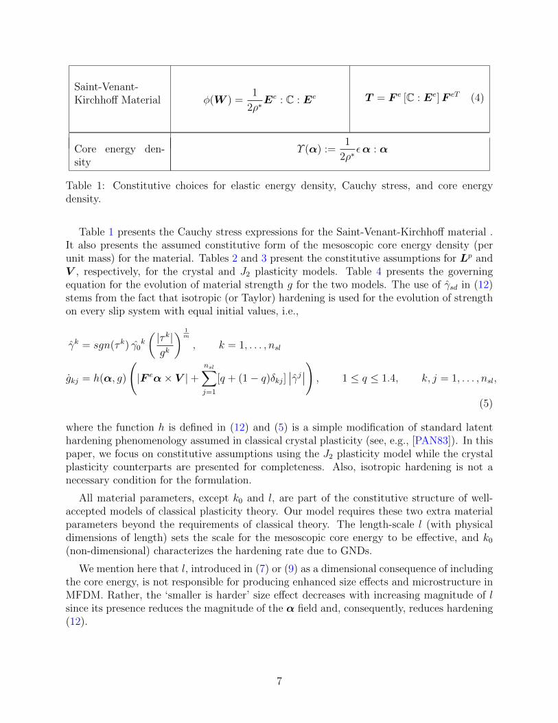
Table 1 presents the Cauchy stress expressions for the Saint-Venant-Kirchhoff material .It also presents the assumed constitutive form of the mesoscopic core energy density (perunit mass) for the material. Tables 2 and 3 present the constitutive assumptions for Lp andV , respectively, for the crystal and J2 plasticity models. Table 4 presents the governingequation for the evolution of material strength g for the two models. The use of γsd in (12)stems from the fact that isotropic (or Taylor) hardening is used for the evolution of strengthon every slip system with equal initial values, i.e.,

γk = sgn(τ k) γ0k

(|τ k|gk

) 1m

, k = 1, . . . , nsl

gkj = h(α, g)

(|F eα× V |+

nsl∑j=1

[q + (1− q)δkj]∣∣γj∣∣) , 1 ≤ q ≤ 1.4, k, j = 1, . . . , nsl,

(5)

where the function h is defined in (12) and (5) is a simple modification of standard latenthardening phenomenology assumed in classical crystal plasticity (see, e.g., [PAN83]). In thispaper, we focus on constitutive assumptions using the J2 plasticity model while the crystalplasticity counterparts are presented for completeness. Also, isotropic hardening is not anecessary condition for the formulation.

All material parameters, except k0 and l, are part of the constitutive structure of well-accepted models of classical plasticity theory. Our model requires these two extra materialparameters beyond the requirements of classical theory. The length-scale l (with physicaldimensions of length) sets the scale for the mesoscopic core energy to be effective, and k0(non-dimensional) characterizes the hardening rate due to GNDs.

We mention here that l, introduced in (7) or (9) as a dimensional consequence of includingthe core energy, is not responsible for producing enhanced size effects and microstructure inMFDM. Rather, the ‘smaller is harder’ size effect decreases with increasing magnitude of lsince its presence reduces the magnitude of the α field and, consequently, reduces hardening(12).

7

Lp = W

(nsl∑k

γkmk ⊗ nk)sym

(6)

Lp = Lp +

(l2

nsl

nsl∑k

|γk|

)curlα (7)

γk = sgn(τ k) γ0k

(|τ k|g

) 1m

(8)

Crystal plasticity

τ k = mk · Tnk; mk = F emk0; nk = F e−Tnk0

J2 plasticity

Lp = γWT′

|T ′ |; γ = γ0

(|T ′|√

2 g

) 1m

Lp = Lp + l2γ curlα (9)

Table 2: Constitutive choices for plastic strain rate due to SDs Lp.

T ′ij = Tij −Tmm

3δij; ai :=

1

3TmmεijkF

ejpαpk; ci := εijkT

′jrF

erpαpk

d = c−(c · a|a|

)a

|a|; γavg =

γ J2 plasticity1

nsl

∑nsl

k |γk| Crystal plasticity.

V = ζd

|d|; ζ =

(µ

g

)2

η2 b γavg (10)

Table 3: Constitutive choices for dislocation velocity V .

8

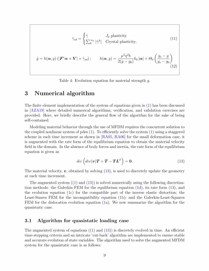
γsd =

γ J2 plasticity∑nsl

k |γk| Crystal plasticity.(11)

g = h(α, g) (|F eα× V |+ γsd) ; h(α, g) =µ2η2b

2(g − g0)k0 |α|+Θ0

(gs − ggs − g0

)(12)

Table 4: Evolution equation for material strength g.

3 Numerical algorithm

The finite element implementation of the system of equations given in (1) has been discussedin [AZA19] where detailed numerical algorithms, verification, and validation exercises areprovided. Here, we briefly describe the general flow of the algorithm for the sake of beingself-contained.

Modeling material behavior through the use of MFDM requires the concurrent solution tothe coupled nonlinear system of pdes (1). To efficiently solve the system (1) using a staggeredscheme in each time increment as shown in [RA05, RA06] for the small deformation case, itis augmented with the rate form of the equilibrium equation to obtain the material velocityfield in the domain. In the absence of body forces and inertia, the rate form of the equilibriumequation is given as

div(div(v)T + T − TLT

)= 0. (13)

The material velocity, v, obtained by solving (13), is used to discretely update the geometryat each time increment.

The augmented system ((1) and (13)) is solved numerically using the following discretiza-tion methods: the Galerkin FEM for the equilibrium equation (1d), its rate form (13), andthe evolution equation (1c) for the compatible part of the inverse elastic distortion; theLeast-Suares FEM for the incompatibility equation (1b); and the Galerkin-Least-SquaresFEM for the dislocation evolution equation (1a). We now summarize the algorithm for thequasistatic case.

3.1 Algorithm for quasistatic loading case

The augmented system of equations ((1) and (13)) is discretely evolved in time. An efficienttime-stepping criteria and an intricate ‘cut-back’ algorithm are implemented to ensure stableand accurate evolution of state variables. The algorithm used to solve the augmented MFDMsystem for the quasistatic case is as follows:

9

• Given the material parameters and initial conditions on α and the prescribed tractiont (most often vanishing), ECDD is used to obtain f , χ, and T on the configuration att = 0.

• Given the geometry and state variables (f t,χt,αt,V n,Lp, and gn) at time tn, ∆tn :=tn+1 − tn is then calculated based on the time stepping criteria explained in [AZA19,Sec. 4]. The following steps are used to evolve the system in a time increment [tn, tn+1]:

1. The rate form of the equilibrium equation (13) is solved on the configurationΩn toobtain the material velocity field vn. This velocity field vn is used to (discretely)evolve the geometry to obtain the configuration at time Ωn+1.

2. The dislocation evolution equation (1a) is solved on Ωn to obtain αn+1 on theconfiguration Ωn+1.

3. χn+1 on Ωn+1 is obtained by solving (1b) with αn+1 as data.

4. fn+1 is determined as follows:

(a) f is evolved from (1c) to obtain fn+1 on the configuration Ωn+1.

(b) In alternate increments, the equilibrium equation (1d) is solved on the config-uration Ωn+1 which is now posed as a traction boundary value problem (withrigid modes eliminated by kinematic constraints). The statically admissiblenodal (reaction) forces, on the part of the boundary with Dirichlet bound-ary conditions on material velocity, are computed following the discussion in[AZA19, Sec. 3.1.1].

5. Once the state at time tn+1 is accepted after checking through the cut-back crite-rion [AZA19, Sec. 4], the above algorithm is repeated to obtain the new state attn+2.

The fields obtained from Steps 3. and 4a. above suffice to define an approximation forthe stress field at tn+1, using the hyperelastic constitutive equation. However, this may notsatisfy (discrete) balance of forces at each time step (because the current geometry obtainedfrom the rate-form of equilibrium and the stress field under discussion need not necessarilybe ‘consistent’ with each other in the sense of discretely satisfying force balance on Ωn+1);therefore we periodically use the discrete equilibrium equation to correct for force balance(Step 4b. above) .

The algorithm above is described in greater detail in [Aro19, AZA19], and has beenimplemented in an MPI(Message Passing Interface)-accelerated C++ code utilizing variouscomprehensive state of the art libraries such as Deal.ii [ABD+17], P4est [BWG11], MUMPS[ADKL01], and PetSc [BAA+17] .

4 Results and discussion

We use the parallel computational framework of MFDM developed in [AZA19] to solve threefundamental problems in finite deformation dislocation mechanics and small-scale plasticity.

10

Before proceeding to discuss results, we mention some details pertaining to our calcula-tions. For all the results presented in this work, the input flux α(V · n) and curlα× n areassumed to be 0 on the boundary. Also, Lp is directly evaluated at the boundary to calcu-late Lp × n. All fields are interpolated using bilinear/trilinear elements in 2-d/3-d, unlessotherwise stated. The Burgers vector content of an area patch A with normal n is givenby bA =

∫Aαn dA, where α denotes the dislocation density field in the domain. When the

dislocation distribution α is localized in a cylinder around a space curve as its axis and thiscylinder threads the area patch A, then we denote its Burgers vector by b. It must be notedthat b is independent of any area patch A for which the intersection of the ‘core’ cylinderand the patch is entirely contained within the patch, this being a consequence of the factthat divα = 0. We refer to the magnitude of the Burgers vector, |b|, as the strength of thedislocation. We define a measure of magnitude of the GND density as [AA19]

ρg(x, t) :=|α(x, t)|

b.

All algorithms in this paper have been verified to reproduce classical plasticity solutionsfor imposed homogeneous deformation histories by comparison with solutions obtained byintegrating the evolution equation (14) for the elastic distortion tensor F e to determine theCauchy stress response for an imposed spatially homogeneous velocity gradient history, L:

F e = LF e − F eLpF e =: f(F e, g),

g = g(F e, g),(14)

where Lp is defined from Eq. (9) or (7) with l = 0, and g is given by (12) with k0 = 0.

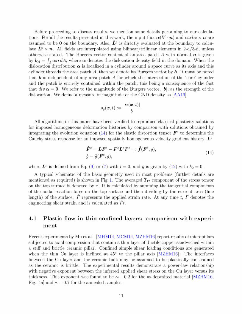
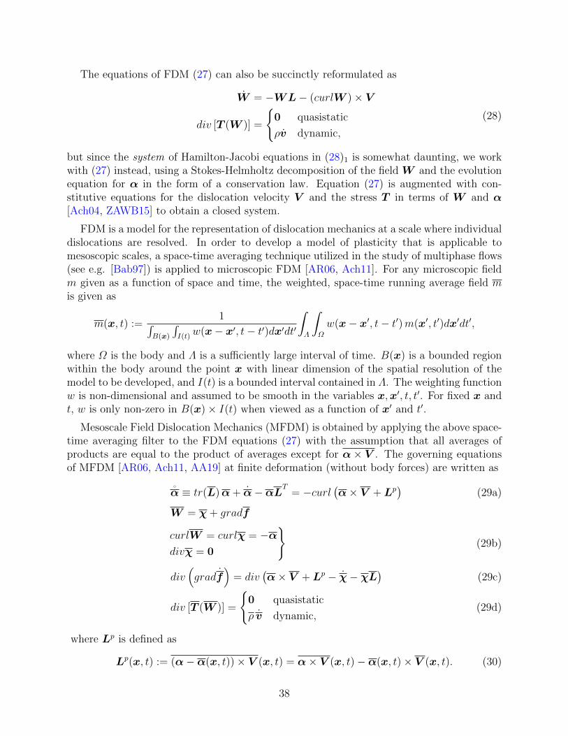
A typical schematic of the basic geometry used in most problems (further details arementioned as required) is shown in Fig. 1. The averaged T12 component of the stress tensoron the top surface is denoted by τ . It is calculated by summing the tangential componentsof the nodal reaction force on the top surface and then dividing by the current area (linelength) of the surface. Γ represents the applied strain rate. At any time t, Γ denotes theengineering shear strain and is calculated as Γ t.

4.1 Plastic flow in thin confined layers: comparison with experi-ment

Recent experiments by Mu et al. [MHM14, MCM14, MZHM16] report results of micropillarssubjected to axial compression that contain a thin layer of ductile copper sandwiched withina stiff and brittle ceramic pillar. Confined simple shear loading conditions are generatedwhen the thin Cu layer is inclined at 45 to the pillar axis [MZHM16]. The interfacesbetween the Cu layer and the ceramic bulk may be assumed to be plastically constrainedas the ceramic is brittle. The experimental results demonstrate a power-law relationshipwith negative exponent between the inferred applied shear stress on the Cu layer versus itsthickness. This exponent was found to be ∼ −0.2 for the as-deposited material [MZHM16,Fig. 4a] and ∼ −0.7 for the annealed samples.

11

𝑣" = $𝛤𝑦

𝒗𝟏 = 𝟎, 𝒗𝟐 = 𝟎

𝑦

𝑃 = (𝑥", 𝑥/)

𝑥"

𝑥/

Top surface

Right surface

Left surface

Bottom surface

𝑣/ = 0

Figure 1: Typical schematic of a rectangular body under shear loading.

As noted in [MZHM16, pp. 5–6] and by Hutchinson [Hut19], and posed as a fundamentalchallenge to all higher-order strain gradient plasticity theories which predict a size effect dueto interface constraints, such models inevitably predict a scaling exponent≤ −1, representinga much stiffer response than observed in experiment.

The situation above has prompted a further formulation of strain gradient plasticity[DO19] introducing a new fitting parameter and adapted to this single experiment, as wellas reformulations [KN19b] of existing SGP models wherein ad-hoc relaxation of boundaryconstraints dictated by the basic theory is suggested to accommodate the observed behaviorwith the justification that “there is a maximum value of the magnitude of the plastic straingradient at the layer boundaries that can be supported before plastic straining starts at theboundary.” Moreover, it is understood from the kinematics of dislocation motion that plas-tic shearing parallel to a boundary is not constrained by constrained plastic flow boundaryconditions [GN05] [AR06, Sec. 2.2.1].

In contrast, here (Sec. 4.1) we use the finite deformation J2 MFDM computational frame-work to model the constrained simple shear of a thin polycrystalline metallic strip withoutany adjustment to the basic model to accommodate this specific experiment. We focus onthe result for the as-deposited material and correspondingly use a reasonable value of theinitial yield stress to reflect the presence of an initial statistical dislocation density in thematerial.

The scaling exponent, denoted by β, is evaluated by assuming a power-law relationship(τ − g0g0

)= cHβ, (15)

where c is a scalar which is constant for a given strain and boundary conditions, and Hdenotes the film thickness. Moreover, since MFDM accounts for the finite deformation stressfields for the GNDs and their spatio-temporal evolution coupled to the underlying kinematics,we also present the microstructure evolution during the deformation.

12

Size (µm× µm) Mesh

5× .50 100× 10

5× .65 100× 13

5× .80 100× 16

5× 1.0 100× 20

Table 5: Mesh details for different domain sizes.

0.0 0.08 0.16 0.24 0.32 0.4

Γ

0.00.00.00.00.00.0

2.25

4.5

6.75

9.0

τ

g0

100× 10

100× 20

Error

100× 10

100× 20

Error0.0

2.0

4.0

6.0

8.0

Err

or%

a: H = 0.5µm

0.0 0.08 0.16 0.24 0.32 0.4

Γ

0.00.00.00.00.00.0

2.25

4.5

6.75

9.0

τ

g0

100× 20

100× 40

Error

100× 20

100× 40

Error0.0

3.5

7.0

10.5

14.0

Err

or%

b: H = 1µm

Figure 2: Convergence of stress-strain responses.

Parameter Value

γ0 0.001s−1

m 0.03

η1

3b 4.05A

g0 .0173 GPa

gs .161 GPa

Θ0 .3925 GPa

k0 20

l√

3× 0.1µm

E 62.78 GPa

ν .3647

Table 6: Parameter values used tomodel the effect of thickness on theflow stress of thin metal films.

13

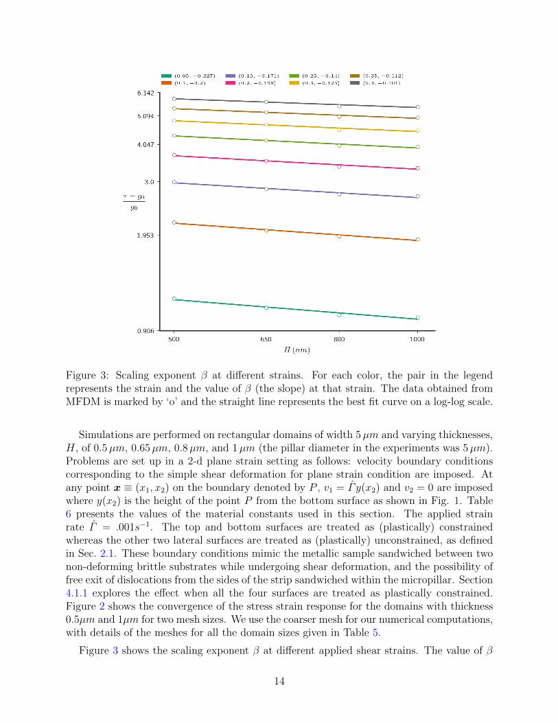
Figure 3: Scaling exponent β at different strains. For each color, the pair in the legendrepresents the strain and the value of β (the slope) at that strain. The data obtained fromMFDM is marked by ‘o’ and the straight line represents the best fit curve on a log-log scale.

Simulations are performed on rectangular domains of width 5µm and varying thicknesses,H, of 0.5µm, 0.65µm, 0.8µm, and 1µm (the pillar diameter in the experiments was 5µm).Problems are set up in a 2-d plane strain setting as follows: velocity boundary conditionscorresponding to the simple shear deformation for plane strain condition are imposed. Atany point x ≡ (x1, x2) on the boundary denoted by P , v1 = Γ y(x2) and v2 = 0 are imposedwhere y(x2) is the height of the point P from the bottom surface as shown in Fig. 1. Table6 presents the values of the material constants used in this section. The applied strainrate Γ = .001s−1. The top and bottom surfaces are treated as (plastically) constrainedwhereas the other two lateral surfaces are treated as (plastically) unconstrained, as definedin Sec. 2.1. These boundary conditions mimic the metallic sample sandwiched between twonon-deforming brittle substrates while undergoing shear deformation, and the possibility offree exit of dislocations from the sides of the strip sandwiched within the micropillar. Section4.1.1 explores the effect when all the four surfaces are treated as plastically constrained.Figure 2 shows the convergence of the stress strain response for the domains with thickness0.5µm and 1µm for two mesh sizes. We use the coarser mesh for our numerical computations,with details of the meshes for all the domain sizes given in Table 5.

Figure 3 shows the scaling exponent β at different applied shear strains. The value of β

14

predicted by MFDM is between 0 and −1 and very close to the value observed in experimentson the as-deposited samples in [MZHM16]. We predict a clear decreasing trend in the valuesof |β| with increasing strain. We note that the predicted values of β are a pure outcomeof the theory unlike [DO19] wherein the scaling exponent is exactly equal to the fractionalorder of the discrete plastic-strain derivatives embedded in their theory, but undeterminedby it.

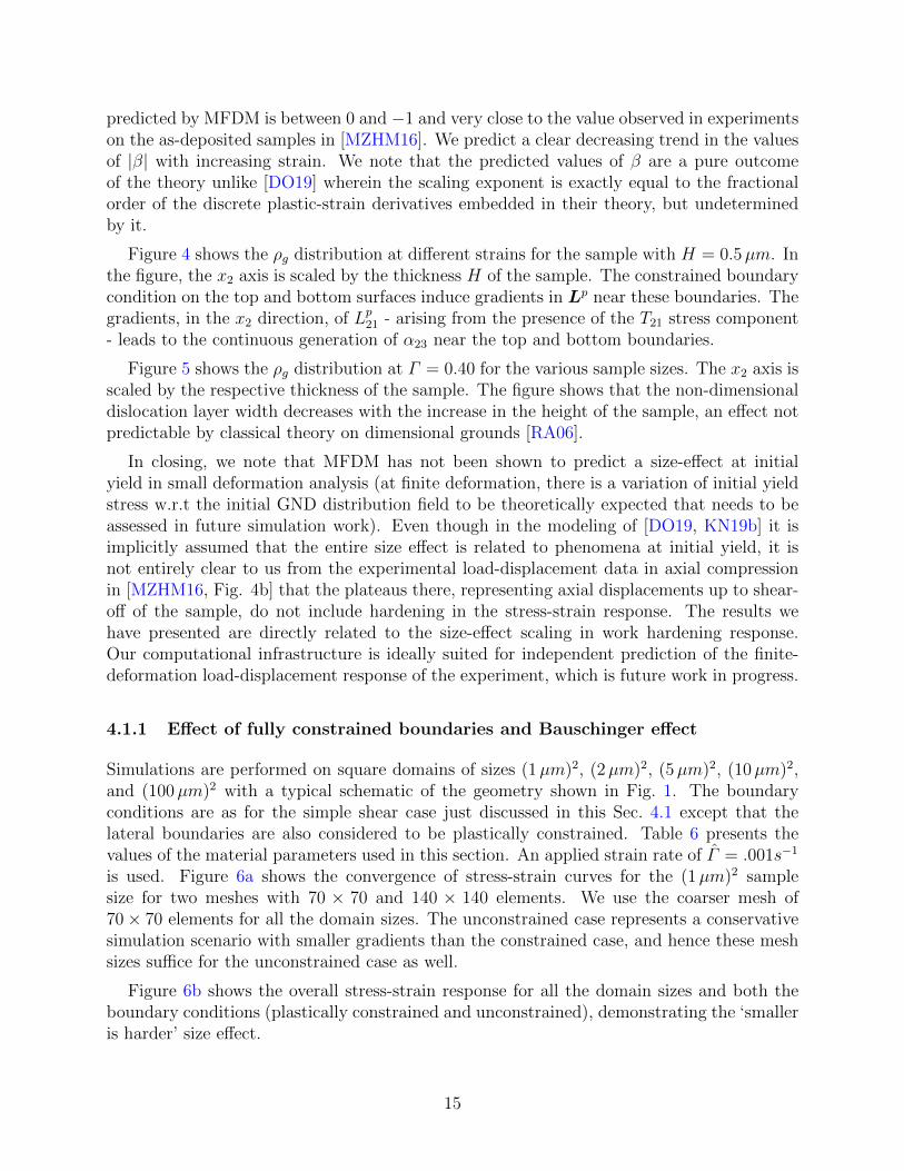
Figure 4 shows the ρg distribution at different strains for the sample with H = 0.5µm. Inthe figure, the x2 axis is scaled by the thickness H of the sample. The constrained boundarycondition on the top and bottom surfaces induce gradients in Lp near these boundaries. Thegradients, in the x2 direction, of Lp21 - arising from the presence of the T21 stress component- leads to the continuous generation of α23 near the top and bottom boundaries.

Figure 5 shows the ρg distribution at Γ = 0.40 for the various sample sizes. The x2 axis isscaled by the respective thickness of the sample. The figure shows that the non-dimensionaldislocation layer width decreases with the increase in the height of the sample, an effect notpredictable by classical theory on dimensional grounds [RA06].

In closing, we note that MFDM has not been shown to predict a size-effect at initialyield in small deformation analysis (at finite deformation, there is a variation of initial yieldstress w.r.t the initial GND distribution field to be theoretically expected that needs to beassessed in future simulation work). Even though in the modeling of [DO19, KN19b] it isimplicitly assumed that the entire size effect is related to phenomena at initial yield, it isnot entirely clear to us from the experimental load-displacement data in axial compressionin [MZHM16, Fig. 4b] that the plateaus there, representing axial displacements up to shear-off of the sample, do not include hardening in the stress-strain response. The results wehave presented are directly related to the size-effect scaling in work hardening response.Our computational infrastructure is ideally suited for independent prediction of the finite-deformation load-displacement response of the experiment, which is future work in progress.

4.1.1 Effect of fully constrained boundaries and Bauschinger effect

Simulations are performed on square domains of sizes (1µm)2, (2µm)2, (5µm)2, (10µm)2,and (100µm)2 with a typical schematic of the geometry shown in Fig. 1. The boundaryconditions are as for the simple shear case just discussed in this Sec. 4.1 except that thelateral boundaries are also considered to be plastically constrained. Table 6 presents thevalues of the material parameters used in this section. An applied strain rate of Γ = .001s−1

is used. Figure 6a shows the convergence of stress-strain curves for the (1µm)2 samplesize for two meshes with 70 × 70 and 140 × 140 elements. We use the coarser mesh of70× 70 elements for all the domain sizes. The unconstrained case represents a conservativesimulation scenario with smaller gradients than the constrained case, and hence these meshsizes suffice for the unconstrained case as well.

Figure 6b shows the overall stress-strain response for all the domain sizes and both theboundary conditions (plastically constrained and unconstrained), demonstrating the ‘smalleris harder’ size effect.

15

(a) (b)

(c) (d)

Figure 4: ρg(m−2) at different strains for the sample with H = 0.5µm.

16

(a) (b)

(c) (d)

Figure 5: ρg at 40% strain for different sample sizes. a) H = 0.5µm b) H = 0.65µm c)H = 0.8µm d) H = 1µm.

0.0 0.08 0.16 0.24 0.32 0.4

Γ

0.00.00.00.00.00.0

2.25

4.5

6.75

9.0

τ

g070× 70

70× 140

Error

70× 70

70× 140

Error

0.0

2.57

5.14

7.71

10.29

12.86

15.43

18.0

Err

or%

(a) Convergence of stress-strain re-sponse for the (1µm)2 domain.

0.0 0.08 0.16 0.24 0.32 0.4

Γ

0.00.0

1.8

3.6

5.4

7.2

9.0

τ

g0

(1µm)2 C

(1µm)2 U

(5µm)2 C

(5µm)2 U

(10µm)2 C

(10µm)2 U

(100µm)2 U

(1µm)2 C

(1µm)2 U

(5µm)2 C

(5µm)2 U

(10µm)2 C

(10µm)2 U

(100µm)2 U

(b) Size effect under simple shear. C: Constrained bound-aries U: Unconstrained boundaries.

17

Figure 7: Scaling exponent β at different strains. For each curve, the trio in the legendrepresents the strain followed by the values of the slope, β, from the left, of the two straightlines comprising the curve. The data obtained from MFDM is marked by ‘o’ and the straightportions of the curves represent the best fit lines of the data on a log-log scale.

Figure 7 presents the scaling exponent β at different strains. The values of β lie between0 and −1 with magnitudes less than the case studied in Figure 3. The data over the wholesize range does not fit a single power law expression; as shown, two power-laws appear toprovide a reasonable fit.

Figure 8a shows the stress strain plot for the (1µm)2 sample size with constrained bound-aries up to 60% strain and Figure 8b shows the ρg distribution at that strain. The loadingdirection is then reversed and the body starts unloading elastically. Fig. 8c shows the ρgdistribution in the domain at 59.17% strain when the averaged load on the top surface (τ)is close to 0. As the reverse loading continues, the body starts deforming plastically againaround 58.65% strain displaying a strong Bauschinger effect, presumably due to the internalstresses of the α distribution. Figure 8d show the ρg distribution at 58.65% strain when theplastic deformation initiates again.

Figure 9 shows the ρg distribution in the same problem at three different strains of 40%,45.46%, and 49.99% during the forward loading. There is considerable development of wall-like microstructure in the interior of the domain between 40%-50% strain. This interior

18

0.1 0.2 0.3 0.4 0.5 0.6

Γ

-11.1

-8.32

-5.55

-2.78

0.00.0

2.6

5.2

7.8

10.4

τ

g0

(1µm)2 C(1µm)2 C

(a) (b)

(c) (d)

Figure 8: a) Stress strain response for (1µm)2 fully constrained (C) sample demonstratingBauschinger effect. The green dotted line shows the elastic unloading curve. b) ρg distribu-tion at 60% strain c) ρg distribution at 0 averaged load on the top surface d) ρg distributionat 58.65% strain when plastic deformation starts again after the loading direction is reversed.

microstructure pattern formation roughly coincides with the ‘wavy’ signature in the stress-strain response beyond 40% strain in Fig. 8a.

4.2 Finite elastic fields in polygonization

We use finite deformation FDM to study the stress and energy density fields of a sequenceof dislocation distributions whose limit is a through-dislocation wall, as observed in thephysical process of polygonization [Gil55, Nab67]. After presenting our results, we makecontact with available mathematical work [MSZ15b, Gin19b] on the limit energy functionalsfor nonlinear elastic deformations with dislocations, show that the current state-of-the-artof mathematical work in this direction is inadequate for the problem of polygonization, anddiscuss our perspective on the problem.

We compute the stress field of a special sequence of dislocations, wherein the dislocationcores stack up to form a dislocation wall in the limit. The result is a tilt grain boundaryconsistent with a piecewise uniform finite rotation field resulting in zero-stresses in the do-

19

(a) (b)

(c)

Figure 9: ρg distribution in the domain at different strains around the onset of ‘waviness’ instress-strain curve Fig. 8a during loading.

20

main. Before analyzing the stress fields for the sequence of dislocation distributions, we firststudy the limiting case, i.e., a polygonized domain with two dislocation walls as shown inFig. 10. The height of the dislocation walls is chosen as 25k where k denotes the width ofthe walls.

25k

50k

x2

x1

θ0 θ0

Dislocation Wall

25k

Figure 10: Schematic layout of the polygonized domain.

x1

θ

θ0

−θ0

25k−25k

Figure 11: Variation of θ in thepolygonized domain for dislocationwalls centered at x1 = ±25k.

In the limiting case, the orientation of the lattice on one side of the wall differs fromthe other side by a rotation angle denoted by θ0. To construct the dislocation density fielddescribing the two walls in the domain for a given θ0, we first approximate this piecewiseconstant rotation angle field by a continuous field

θ(x) = −θ02

[tanh

(x1 + 25k

a k

)+ tanh

(x1 − 25k

a k

)], (16)

with the walls centered at x1 = ±25k, and a is a dimensionless scalar chosen to be 0.238which ensures that the widths of the dislocation walls are k. Figure 11 shows the variationof θ(x) along x1 in the polygonized domain. The corresponding elastic distortion F e is thengiven by the rotation tensor field

F e(x) =

cos(θ(x)) − sin(θ(x)) 0sin(θ(x)) cos(θ(x)) 0

0 0 1

, (17)

with the corresponding dislocation density field in the domain given by α = −curlW .

A non-uniform mesh, highly refined close to the dislocation walls, is used to discretizethe polygonized domain comprising an isotropic Saint-Venant-Kirchhoff elastic material withE = 200GPa and ν = 0.3. The stress fields are calculated for θ0 = 45 in a 2-d plane strainsetting. Since θ does not vary in the x2 direction

α13 = −ε312 (W )12,1 = cos(θ)dθ

dx; α23 = −ε312 (W )22,1 = sin(θ)

dθ

dx.

Thus, α23 ≈ 0 is a reasonable approximation for low-angle grain boundaries. The solution forthe nonlinear elastic stress field of the chosen F e field is of course trivial - it is 0 everywhere.However, the stress field of a progressively forming dislocation wall whose elastic distortion

21

(a) (b)

Figure 12: a) α13 b) α23 in the polygonized domain with θ0 = 45.

approaches a rotation tensor field everywhere is non-trivial, as we show in the following.Since the latter is our main interest, and the knowledge of the trivial solution does nothelp in solving the latter problem, we devise a unified strategy to solve the entire class ofproblems. This requires first to solve the ‘full-wall’ problem with the trivial solution by anon-trivial method that then finds crucial use in solving the full range of ‘sparse’ to ‘full’wall problems. In what follows, we first describe how the full-wall problem is dealt with.

With the dislocation density field and vanishing applied tractions specified, the ECDDsystem (2)-(3) is solved in the polygonized domain to determine the stress field. The nu-merical solution of the nonlinear ECDD problem requires a good initial guess. This guessis obtained by solving for f by using the Least-Squares finite element method with objec-tive functional 1

2

∫Ω||gradf + χ −W ||2 dV with W and χ specified. The specified data is

generated from W , the inverse elastic distortion field corresponding to the prescribed F e

field given by (17), and by solving for χ from the div-curl system (1b) with α = −curlWspecified. The weak form (to solve for f) is given by∫

Ω

gradf : gradδf dV =

∫Ω

(W − χ) : gradδf dV. (18)

f is fixed at one point in the domain to obtain a unique solution. Solving for f from theleast squares method implies (W −χ)n = (gradf)n holds weakly on the external boundary.

Figure 13 shows the distribution of the T12 stress component in the domain, with thedislocation density fields shown in Figure 12. As can be seen, the shear stresses are negligiblein the entire domain and further decrease upon refinement. To verify that the values of allthe components of the stress tensor T are negligible, we define two non-dimensional measuresof strain energy density in the domain as follows:

ψfd =1

2µEe : C : Ee; Ee =

1

2(F eTF e − I) (19)

ψsd =1

2µ(F e − I) : C : (F e − I). (20)

In the above, ψfd and ψsd denote the finite and small deformation non-dimensional strainenergy densities, respectively. Figure 14 shows the distribution of finite deformation strainenergy density ψfd in the domain. The negligible magnitude of the ψfd distribution in

22

Figure 13: T12 in the polygonized domain with θ0 = 45.

Figure 14: Finite deformation strain energydensity ψfd in the polygonized domain.

Figure 15: Small deformation strain energydensity ψsd in the polygonized domain. Forthe region where the normalized energy den-sity ψsd > 5× 10−4, the value is 0.4.

the body demonstrates that the body is stress-free. However, Figure 15 demonstrates thatthe small deformation theory predicts a non-zero strain energy density profile even when thevalues of the elastic distortion field is a rotation tensor everywhere. Moreover, the expressionfor the strain energy density for the small deformation (linear) theory is not invariant undersuperposed rigid body motions.

We now demonstrate the stress and energy density field paths induced by a sequence ofdislocation distributions, going from one core to a full wall, in a rectangular domain of size100k × 50k. The θ(x) corresponding to a dislocation wall centered at x1 = 0 is given by

θ(x) =θ02

[1− tanh

( x1a k

)], (21)

where θ0 is the rotation angle, equal to the difference in the orientations of the lattice acrossthe wall. Equation (17) gives the elastic distortion tensor field in the domain. The values ofa and θ0 are chosen to be same as in the previous section, i.e. 0.238 and 45, respectively. Asbefore, the negative curl of the inverse elastic distortion field gives the dislocation densitycomprising the full dislocation wall. The dislocation density field corresponding to a singlecore amounts to isolating the dislocation density distribution in a region of dimension k× kfrom the full wall, with value 0 everywhere else in the domain. The dislocation densitycorresponding to multiple cores in a wall configuration can then be prescribed by using thedislocation density field corresponding to the single core with a vertical shift and aligningthe so-obtained core with the previous ones. For any given number of dislocation cores inthe rectangular body, denoted by nc, the ECDD system is solved to obtain the stress fieldin the body. The chosen sequence of positions and number (of cores) for the α13 componentof the dislocation density is shown in Figure 16. α23 is similarly placed and its values are

23

Figure 16: Position of dislocation cores comprising the progressively developing dislocationwall.

accordingly assigned. The Burgers vector for a single dislocation core is computed to beb = .778k e1 − .322k e2. A uniform mesh of (0.1k)2 sized elements is used to discretize therectangular domain for all cases except for the case of nc = 50. For nc = 50, the mesh isfurther refined near the dislocation wall.

For the simulations with nc ≤ 30 the initial guess to the Newton-Raphson method is ob-tained from the small deformation equilibrium problem solved on the current configurationas discussed in [ZAP18, Aro19]; in solving problems of finite deformation dislocation fieldswith sparsely distributed individual dislocations, this is found to be essential. However, forthe simulations with nc ≥ 36, the initial guess is obtained by solving (18) (correspondingto a full dislocation wall), and this is also found to be essential to obtain a solution for thestress fields of these ‘dense’ distributions of individual dislocations. For nc = 35, the numer-ical solution did not converge with initial guess coming from either of the two approachesmentioned above. For nc = 32, a solution, using the initial guess from the small-deformationtheory, can be obtained. The same procedure does not succeed for nc = 33, 34.

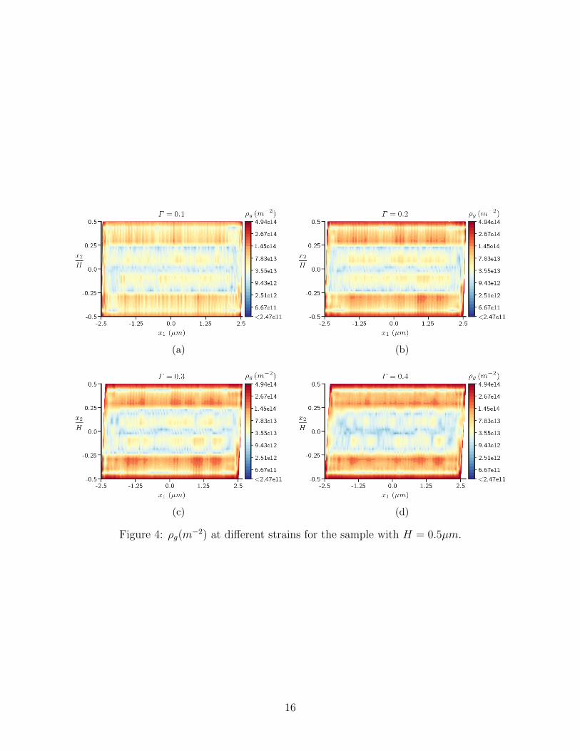
Figures 17 and 18 show the distribution of the T12 stress component and the finite de-formation strain energy density ψfd fields in the body for different number of dislocationcores. An interesting feature of our calculations displayed in Figures 17 and 18 is that thereis a drastic change in the stress and the strain energy distributions when the number of

24

Figure 17: T12 distribution in the domain for different number of dislocation cores. Thecolorbar for the cases nc < 50 is shown at the bottom.

25

Figure 18: ψfd distribution in the domain for different number of dislocation cores. Thecolorbar for the cases nc < 50 is shown at the bottom.

26

Figure 19: Mapping of e1 vector by the calculated elastic distortion field F e.

cores nc ≥ 36. The variation (for both T12 and ψfd) which was spread out in the entiredomain suddenly becomes localized near the wall and the boundary when nc ≥ 36. It isclear that when the number of (same sign) dislocations in the body increases from 0, thestress and energy have to increase. It is also clear that the full wall must represent a stressand energy-free configuration. Whether the transition between these behaviors has to be anabrupt ‘phase transition’ (w.r.t. the number of cores), as indicated by our calculations, is aninteresting question for further study. When θ0 is reduced, the magnitudes for the stress andenergy fields become less pronounced with the qualitative conclusions remaining the same.

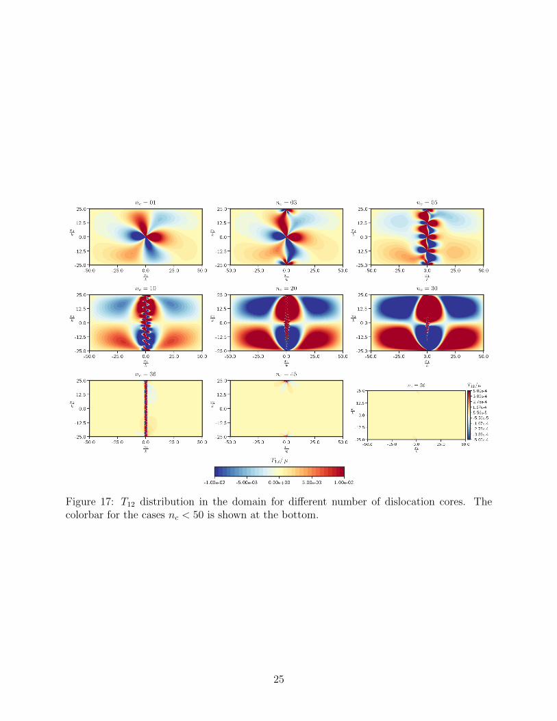
Figure 19 shows the image of the constant e1 vector field under mapping by the elasticdistortion field on the current configuration for the full dislocation wall. We can see thatthe lattice on the left of the dislocation wall is rigidly rotated w.r.t. the lattice on the rightby the prescribed misorientation angle θ0. We also calculate the change in volume (per unitlength of the domain in the e3 direction, i.e. the change in area) of the body due to thepresence of the dislocation wall as described in Sec. 4.3. The % change in volume evaluatesto 0 up to machine precision, a necessary condition for the elastic distortion field to be arotation tensor field (which is spatially inhomogeneous in this instance).

4.2.1 Contact with the mathematical literature

In closing this section, we make contact with the mathematical results of [MSZ15b, Gin19b].A summary of the main result of [MSZ15b] adequate for the present context is as follows:Given a frame-indifferent elastic energy density function W and ε a nondimensional measureof the magnitude of the Burgers vector of a dislocation proportional to a lattice constant ofa crystal,

1

ε2| log ε|2

∫Ω

W (F eε ) dV −→ 1

2

∫Ω

β : Cβ dV +

∫Ω

ϕ(Re,µ) dV, (22)

where F eε is a sequence of elastic distortions consistent with a corresponding sequence of

discrete dislocation distributions in the body given by µε through curlF eε = µε, µε → µ,

there exists a sequence of spatially constant rotation fields Reε → Re such that ReT

ε Feε −I →

β with |ReTε F

eε − I| = O(ε| log ε|), and curlβ = ReTµ, C is the standard linear elastic

moduli (with minor (and major) symmetries), ϕ is a function that is deduced, and all

27

Screw dislocation with Burgers vector magnitude bBody radius RCore radius ~ Interatomic spacing b

Figure 20: Physical length scales for a single dislocation in a finite body

arrows represent appropriate (scaled) convergences as ε → 0. Furthermore, an importanthypothesis, for this discussion, on the ‘well-separated’ness of admissible discrete dislocationdistributions is that for any two dislocations comprising µε located at x and y, |x−y| > 2ρε,where “ρε ε, with ρε → 0 as ε→ 0.” That the sequence of rotation tensors Re

ε with limitRe exists for the sequence F e

ε (consistent with admissible µε) is predicated on the assumptionthat the energy of the sequence as ε→ 0 is bounded, i.e.,

supε→0

1

ε2| log ε|2

∫Ω

W (F eε ) dV <∞. (23)

Clearly, for the case of polygonization involving a single dislocation wall as we haveconsidered, a representative sequence F e

ε would have to converge to a rotation field that isnot spatially uniform. Consequently, such a sequence would not be within the purview of theresult of [MSZ15b], since the β for this sequence is neither skew-symmetric nor 0 so that thefirst term on the RHS of (22) does not vanish whereas the limit of the LHS of (22) does forthis sequence. Thus, this failure has to be related to the assumptions behind the [MSZ15b]analysis. Since such hypotheses, and assumptions of the same ilk, are commonplace inthe mathematical literature on dislocations [GLP10, Gin19a, Gin19b, LL16] and has begunto find prominence in the mechanics/engineering literature as well [RSC16, RDOC18], wediscuss them here and provide our perspective on the matter.

First, we clarify an issue that is very rarely addressed in the literature (cf. [RSC16,RDOC18]), which, nevertheless, is crucial for understanding the physical setting of themathematical results. This relates to the use of a fixed, bounded configuration contain-ing dislocations whose strengths are assumed to scale with ε→ 0. With reference to Fig. 20,we first note that the total energy of the cylinder of length L with a single screw dislocationis given by E =

∫ L0

∫ 2π

0

∫ Rbµb2r−2 rdrdθdl, and with the definition ε = bR−1,

E

µ2πL= R2

(b

R

)2

| log ε|.

The energy content of the body can be interpreted in two different non-dimensional limitsas ε→ 0, corresponding to the expressions

E

µ2πLR2= ε2| log ε| and

E

µ2πLb2= | log ε|.

The first considers the body to be of fixed radius R with the interatomic spacing of thecrystal b → 0 in which case the limiting total energy of a dislocation in the body vanishes.

28

With this physical interpretation of ε→ 0, the ε2| log ε|2 scaling employed by [MSZ15b] maybe interpreted, but not necessarily, to correspond to a ‘weakly unbounded’ population ofdislocations in the body growing as | log ε| as ε→ 0 [GLP10, Gin19a, Gin19b] (we discuss adifferent physical interpretation of this ‘fixed body scaling’ in the next paragraph). We note,however, that for a physically realistic, non-degenerate scenario where a single dislocation ina body does not result in 0 internal stress and elastic strain energy regardless of its size, theinteratomic spacing of a crystal is a finite, well-defined physical length for a specific material,as are the dimensions of a body, so choosing ε = b

R→ 0 with R fixed does not appear to be

a viable proposition to us (when considering a fixed material).

On the other hand, keeping b fixed and sending R→∞ seems eminently reasonable (thelimit of a progressively large body of the same material), in which case the total energy of thebody containing the single dislocation diverges as | log ε| → ∞ as ε→ 0. We believe that itis this physically realistic scaling that should be employed in the analysis of dislocations andtheir distributions, with the minimum energy scale being supε→0

1b2| log ε|

∫ΩεW (F e

ε ) dV <∞(the domain depends on ε as it grows in size scaled by bε−1 and we refer to fields on thegrowing domains with an overhead ˜). By the nondimensionalization given by x = xε

bwith

the corresponding domain of fixed size represented by Ω, it can be seen that∫ΩεW (F e

ε ) dV =b2

ε2

∫ΩW (F e

ε ) dV , with F eε (x) = F e

ε (bε−1x), µε(x) = µε(bε−1x), curlF e

ε (x) = ε−1µε(x)1. Itis in this sense that we interpret all ‘fixed domain’ dislocation-related asymptotic resultswith discrete dislocation strengths tending to 0, noting, in particular, the large differencebetween

∫ΩW (F e

ε ) dV and the physical energy content∫ΩεW (F e

ε ) dV as ε→ 0.

Consider now a ‘full’ dislocation wall described by a piecewise constant rotation field (asconstructed in our computational example, but now with a sharp boundary) in a sequenceof square domains of size H × H, with H steadily increasing, representing a progressivelylarge domain containing a bicrystal. The magnitude of the Burgers vector of each individualdislocation in the wall is assumed to be b. Then the result of the case 1

ε= H

b 1 may be

approximated by the results of Hb→ ∞, b fixed. At least within the mathematical context

being considered, the entire sequence of domains has 0 elastic energy (i.e. the part comingfrom W ), which is certainly O of any of the energy bounds ε2| log ε| or ε2| log ε|2 as ε → 0.Moreover, it can be checked that, on the non-dimensional domain of fixed size, the strengthof the Burgers vector of individual dislocations indeed scales like εb, if b is the magnitudeof the Burgers vector of the dislocations on the physical sequence of domains. Why thendoes the elastic part of the limit energy in (22) fail to predict the energy content of such awall, a commonly observed dislocation configuration, well worthy of prediction? The answermust lie in the fact that the ‘full wall,’ while being a very low-energy configuration, cannotbe achieved as a limit configuration of the admissible dislocation sequences allowed by the[MSZ15b] analysis due to the ‘well-separated’ness assumption - indeed, it is, in a sense, an‘opposite’ limit that is considered in our computational example where the core dimensions

1It is presumably based on this correspondence between the non-dimensionalized problem on the fixeddomain and the growing domain problem that [MSZ15a, Gin20] state that “From the point of view of physicsit is more natural to fix the lattice spacing and to consider domains 1

εΩ of increasing size. Upon elasticityscaling both points of view are equivalent and fixing Ω rather than the lattice spacing is more convenientfor the analysis. Thus ε really is a dimensionless parameter of the order of lattice spacing divided by themacroscopic dimension of the body. For brevity we will nonetheless often refer to ε as the lattice spacing.”

29

remains fixed and the inter-core distances reduce to 0. An interesting feature of this specificexample is that the number of dislocations in a configuration (when the core radius tendsto 0) does not correlate, even roughly, with the total energy content of the configuration, asmight be expected based on energy scales related only to self-energy of single dislocations,an argument valid in relatively ‘dilute’ limits [GLP10, Gin19a, Gin19b]. Indeed, the definingenergetic feature of the ‘full wall’ is that the entire energy of the individual dislocations inthe wall gets screened by the ‘(nonquadratic) interaction energy’ between them resulting ina very low-energy state.

Unlike Equation (2.4), Proposition 4.3, and Theorem 4.6 of [MSZ15b], the GeneralizedRigidity Estimate (GRE) [MSZ15b, Theorem 3.3] does apply to the ‘full wall’ configurationunder discussion. It is instructive to understand the breakdown of that result in validating theelastic part of the limit functional in (22) for the specific example of the full dislocation wall.As mentioned earlier in conjunction with (22), for admissible sequences (µε,F

eε ) satisfying

the energy bound (23), |ReTε F

eε−I| is small so that a quadratic approximation of W estimates

it well and it is that quadratic approximation of W with argument β that appears in (22).For the ‘wall sequence’ (on the growing domains, and recalling that b

H=: ε) with constant

unit tangent to the wall in the the direction e2, |U eε − I| is small (actually 0), where U e

ε is

the right stretch tensor of the polar decomposition of F eε and the question becomes as to

whether the spatially non-uniform rotation tensor field of F eε can be approximated well by

a constant rotation Reε in the domain Ωε so that U e

ε can be well approximated by Reε

TF eε .

We are unable to deduce the necessary control on the point-wise values of Reε− F e

ε from theGRE, given here, for each fixed ε, by∣∣∣∣∣∣F e

ε − Reε

∣∣∣∣∣∣L2(Ωε;R2×2)

≤ C(Ωε)

(∣∣∣∣∣∣dist(F eε , SO(2)

)∣∣∣∣∣∣L2(Ωε)

+∣∣∣curl Fε∣∣∣ (Ωε)

)since, although the F e

ε is a rotation tensor field for this specific sequence taking exactly two

distinct values, say Reε1 6= Re

ε2, the various ingredients of the GRE in this specific exampleare given by ∣∣∣∣∣∣F e

ε − Reε

∣∣∣∣∣∣L2(Ωε;R2×2)

=H√

2

√∣∣∣Reε1–R

eε

∣∣∣2 +∣∣∣Re

ε2–Reε

∣∣∣2 6= 0∣∣∣∣∣∣dist(F eε , SO(2)

)∣∣∣∣∣∣L2(Ωε)

= 0∣∣∣curl Fε∣∣∣ (Ωε) = H∣∣∣(Re

ε1 − Reε2

)e2

∣∣∣ ,and the constant C(Ωε) depends on the domain; for the corresponding problem on the fixed-domain, the point-wise squared magnitude of the difference Re

ε−F eε is therefore bounded at

most by anO(1) quantity independent of ε (it is physically obvious that no theorem can provethat the rotation field of a high-angle, symmetric tilt boundary can be well-approximated bya constant rotation everywhere). In case such an approximation were to actually fail, then a‘quadratization’ of W (about 0) is not a good approximation for it, and the limit functionalin (22) cannot be the correct one for this wall sequence. Predictions of such a model would

30

be similar in spirit to what is shown, e.g., in Fig. 15. Interestingly, however, the limit elasticfunctional in (22) is invariant under superposed rigid deformations.

The above arguments also seem to suggest that for small enough energy scales a bettertarget for the elastic part of the limit functional is 1

2

∫Ω

(U e − I) : C(U e − I) dV , whereU eε → U e as ε→ 0, which is invariant under superposed rigid deformation as well as succeeds

for the case of the dislocation wall. However, it should be noted that in the presence of large‘infinities’ of dislocations of sufficient strength, control on the energy (and hence the elasticstrain field) does not control the rotation field, this being expected since such control is ahallmark of compatibility of deformations, as in (non)linear elasticity theory without linedefects.

Finally, in the context of energy scales of dislocation configurations for asymptotic anal-ysis, the highest energy scales that have been considered, to our knowledge, are

supε→0

1

ε

∫Ω

W (F eε ) dV <∞ [LL16] and sup

ε→0

∫Ω

W (F eε ) dV <∞ [RSC16, RDOC18]2;

in both cases, no limit energy functional is deduced as in the other references mentioned,and no (approximate) methods for computing stress fields of the dislocation distributionsare devised.

4.3 Volume change due to dislocations

A fundamental question that was asked by Toupin and Rivlin [TR60] concerns the change involume of a body when dislocations are introduced; linear elastic theory is not capable of cap-turing this volume change, due to the fact that the average value of each of the infinitesimalstrain components of a self-equilibrated stress field in a body vanishes. However, it has beenobserved experimentally that the volume of the body changes upon the introduction of dis-locations [Zen42] and the prediction by linear elastic theory (of no volume change) does notseem to be in agreement with experimental observations. Toupin and Rivlin [TR60] used asecond-order approximation of nonlinear elasticity to give explicit expressions for the changesin average dimensions of elastic bodies resulting from the introduction of dislocations.

Here, we use finite deformation FDM to capture this volume change. The problem is setup in a 2-d plane strain setting as follows: Edge dislocations are assumed to be present ina rectangular body of dimensions [−10b, 10b] × [−10b, 10b]. An edge dislocation, with corecentered at point p = (p1, p2), is modeled by prescribing a dislocation density of the form

α13(x1, x2) =

φ0 |x1 − p1| ≤ b

2and |x2 − p2| ≤ b

2

0 otherwise, αij = 0 if i 6= 1 and j 6= 3. (24)

The constant φ0 is evaluated by making the Burgers vector of the dislocation core equal tobe1, i.e.

∫Ωα13da = b. The external boundaries are assumed to be traction-free. The body

2To appreciate the difference between the energy scales implied by the various scalings considered here(constant, ε, ε2| log ε|, ε2| log ε|2), it is instructive to choose the value ε = 10−10 corresponding to anAngstrom scale interatomic spacing in a body of nominal dimension 1m.

31

(a) (b) (c) (d) (e)

(f) (g) (h) (i)

Figure 21: Figures a-e show the α distributions for the case when the total strength of alldislocations is positive: a) 1 core b) 2 cores c) 4 cores d) 6 cores e) 8 cores. Figures f-i showthe α distributions for the case when the total Burgers vector is zero: f) 2 cores g) 4 coresh) 6 cores i) 8 cores. The legend colorbar is common to all the plots.

is assumed to behave as an isotropic Saint-Venant-Kirchhoff elastic material with E = 200GPa and ν = 0.3.

The volume change is calculated as follows: The ECDD system (2)-(3) is solved on thecurrent configuration to obtain the inverse elastic distortion field for a given dislocationdensity in the domain. The % volume change is then calculated from (25) where Vref andVcurr denote the volume of the reference and the current configurations, respectively:

Vcurr =

∫Ω

dV ; Vref =

∫Ω

det(W ) dV (25a)

∆V = Vref − Vcurr ; %∆V =|∆V |Vcurr

× 100. (25b)

In the following, we present the volume change (per unit length along the e3 axis) approx-imation for two cases corresponding to the total Burgers vector of all the dislocations beinga) positive and b) zero. Table 7a shows the % change in the volume of the body consequentupon the introduction of multiple dislocations of the same sign, distributed in the body asshown in Figures 21a - 21e. Table 7b shows the % change in the volume of the body due tothe introduction of multiple pairs of dislocations, distributed in the body as shown in Figures21f - 21i, such that the total Burgers vector of all dislocations is 0. The configurations forzero resultant Burgers vector utilize positive and negative straight edge dislocation.

Tables 7a and 7b show that the change in volume upon introduction of dislocations asquantified by finite deformation FDM is very small for both the cases. Moreover, we seethat this volume change is not linear w.r.t the number of cores i.e., the change in volumein the presence of 6 dislocations is not the same as 3 times the change in volume when 2dislocations are present. The nonlinearity of the ECDD system and interaction among thedislocations cause the deviation from linear response to give smaller values.

32

Cores %∆V1 .10192 .20644 .30136 .39028 .6025

(a)

Cores %∆V2 .17934 .29386 .35238 .5873

(b)

Table 7: Volume change in body when the resultant strength of all the dislocations is a)positive b) zero.

This study suggests that for an isotropic Saint-Venant-Kirchhoff material, the volumechange calculated with nonlinear theory is very small and therefore the linear theory predic-tion of no volume change is a very good approximation.

4.4 Non-uniqueness of inverse deformation in classical finite elas-ticity with dislocations

Consider the case when a dislocation with Burgers vector b is assumed to be present in thebody. The solution to the ECDD system (2)-(3) on the current configuration Ω gives theinverse elastic distortion field W in the domain. It can be shown that if the dislocationcore is removed from the body and a cut is made that runs from the boundary of the coreto the external boundary of Ω to produce a simply connected body Ωs, then there exists adeformation y of this Ωs such that

gradsy = W , (26)

where W−1 =: F e and grads denotes the gradient on Ωs. The reference configuration is thenobtained by mapping this ‘hollowed and cut’ configuration Ωs by the field y. Moreover, thefield y has two important properties: i) the jump in the value of y (denoted by JyK) alongthe cut surface is equal to the Burgers vector b of the embedded dislocation in the originalbody Ω and, ii) JyK is independent of the cut surface chosen as well [ZA18].

Section 4.4.1 shows that the above topological properties are preserved in the frameworkof (computational) FDM. More interestingly, we are easily able to do similar calculations fora body containing multiple dislocations when the current configuration cannot be renderedsimply-connected by a single cut, as shown in Sec. 4.4.2 – in this case we show that the jumpin y is not constant along the boundary, corresponding to the cuts, of the simply-connecteddomain, in contrast to the single dislocation, single-cut case.

4.4.1 Inverse deformation for a single dislocation

We obtain non-unique reference configurations of a body Ω with a single dislocation withBurgers vector b = be1. The body Ω is made simply connected by removing the core and

33

(a) (b) (c)

(d) (e) (f)

Figure 22: Reference configurations when the cut surface is chosen at varying angles fromthe e1 axis: a) 0 b) 45 c) 135 f) 210 i) 270 j) 315. The Burgers vector is identical forall the cases, while the overall reference configurations are non-trivially different.

making a straight cut, at some angle from the e1 axis, that runs from the boundary of thecore to the external boundary. The field y on this simply connected configuration Ωs iscalculated by using the Least-Squares FEM. Figure 22 shows the reference configurations forthe cut surface chosen at varying angles w.r.t. the e1 axis.

The reference configurations self-penetrate when the cut makes an angle between 0 and180 with the e1 axis. When the angle lies between 180 and 360, the reference configurationsshow detachment. Also, the reference configurations shown in Figures 22b and 22c, and 22aand 22e are entirely different, even though the corresponding simply connected configurationsfor these cases are related by a rigid rotation of −/ + 90 about the e3 axis. This is aconsequence of the constraint that the (vectorial) jump in y has to remain constant alongthe cut surface. Moreover, this jump is exactly equal to the Burgers vector be1 of thedislocation in the original configuration Ω. The jump in the value of the field y is identicalfor all the cuts showing that the jump is independent of the cut surface, thus verifying theexpected topological property.

4.4.2 Inverse deformations for multiple dislocations

This section explores the possibility of obtaining non-unique reference configurations of abody with multiple dislocations. Figure 23 shows such a scenario when 4 dislocations areassumed to be present in the body and reference configurations are obtained by solving fory using the Least-Squares FEM for different simply connected configurations.

34

(a) (b) (c) (d)

(e) (f) (g) (h)

Figure 23: Non unique reference configurations (on the bottom) obtained for different simplyconnected configurations (on the top).

On the top of Figure 23, we show different simply connected configurations, each obtainedby making multiple cuts (shown in red) in Ω. The corresponding reference configurationsare shown on the bottom in Figure 23. As can be seen from these figures, the referenceconfiguration is non-unique - for a given self-equilibrated W - as it depends on the cutsmade in the body to make it simply connected. Moreover, even when the cut-configurationsdiffer by rigid rotations (for example 23a and 23d, and 23b and 23c), the correspondingreference configurations (23e and 23h, and 23f and 23g,) are entirely different. Anotherimportant thing to note here is that unlike the case of the single dislocation, the jump in yis not constant along the cut in the presence of multiple dislocations, but is constant alongthe cut between any two cores, in accord with the analytical values they should take in theseexamples of configurations with multiple cuts.

The above examples highlight an important feature of the ECDD formulation – if the dislo-cation stress problem for specified dislocation density is formulated classically, i.e., involvingonly an inverse deformation field y on the ‘deformed’ configuration with the dislocation con-sidered given, it is clear that there is massive non-uniqueness of solutions y for the samestress field corresponding to W 3; ECDD suffers from no such ambiguity and lends itself torobust computation.

3In the absence of dislocations this corresponds to the classical inverse problem of nonlinear elasticitywhere the deformed, stressed configuration is assumed given with specified traction boundary conditionsand enough kinematic constraints to prevent superposed rigid (inverse) deformation, and the question is todetermine the stress-free elastic reference by solving for the inverse deformation.

35

5 Conclusion

A partial differential equation based model of finite deformation plasticity coupled to dis-location mechanics has been presented, with no restriction on material and geometric non-linearities. The model fundamentally accounts for the stress field of arbitrary dislocationdistributions and melds elastic dislocation theory at finite deformation with J2 plasticity ina practical manner suitable for application. This paper along with [AA19, AZA19] forma trio that solves some key problems of current and classical significance in the fields ofplasticity and dislocation mechanics, utilizing a finite element based computational frame-work developed in [AZA19]. As well, Lauteri and Luckhaus [LL16] state “It is worthwhileto compare our result with the differential geometric description of dislocation structures,introduced by Kondo, Kroner and Bilby at al. (see [Kon64, Kro59, BBS55]) and also withΓ-limit results in the context of linear elasticity where implicitly or explicitly a volume den-sity of dislocations is assumed (see [GLP10]). It remains to be investigated if these modelsremain valid as averaged limits if on an intermediate scale there exists a Cosserat structureof micrograins.” - up to the intended meaning of “averaged limits” above, we believe thatwe have answered this latter question in the affirmative, albeit with a far-reaching extensionof the pioneering differential geometric works, going beyond simply kinematic considerationsat finite deformations. We believe that our work provides a practical pathway for exploringmany problems at the intersection of finite deformation plasticity and dislocation mechan-ics at realistic length and time scales. Further work will involve probing problems of shearlocalization in 2 and 3 dimensional bodies of rate-dependent and rate-independent mate-rials, among others. Finally, improving the constitutive assumptions inherent in Lp basedon averaging of dislocation dynamics at the individual defect scale remains a fundamentalpursuit.

Acknowledgments

This research was funded by the Army Research Office grant number ARO-W911NF-15-1-0239. This work also used the Extreme Science and Engineering Discovery Environment(XSEDE) [TCD+14], through generous XRAC grants of supercomputing resources, whichis supported by National Science Foundation grant number ACI-1548562. We gratefullyacknowledge the Pittsburgh Supercomputing Center (PSC), and Prof. Jorge Vinals and theMinnesota Supercomputing Institute (URL: http://www.msi.umn.edu) for providing com-puting resources that contributed to the research results reported within this paper. It is agreat pleasure to acknowledge insightful discussions with Janusz Ginster and Reza Pakzad.

Appendix A (Mesoscale) Field Dislocation Mechanics

(M)FDM

Significant portions of this section are common with [AA19, AZA19], papers developedconcurrently with this work. We include this material here for the sake of being self-contained

36

and since the theory being discussed is quite recent.

Field Dislocation Mechanics (FDM) was developed in [Ach01, Ach03, Ach04, Ach07] build-ing on the pioneering works of Kroner [Kro81], Willis [Wil67], Mura [Mur63], and Fox [Fox66].The theory utilizes a tensorial description of dislocation density [Nye53, BBS55], which isrelated to special gradients of the (inverse) elastic distortion field. The governing equationsof FDM at finite deformation are presented below:

α ≡ tr(L)α+ α−αLT = −curl (α× V ) (27a)

W = χ+ gradf ; F e := W−1

curlW = curlχ = −αdivχ = 0

(27b)

div(gradf

)= div (α× V − χ− χL) (27c)

div [T (W )] =

0 quasistatic

ρv dynamic.(27d)

Here, F e is the elastic distortion tensor, χ is the incompatible part of W , f is the plasticposition vector [AR06], gradf represents the compatible part of W , α is the dislocationdensity tensor, v represents the material velocity field, L = gradv is the velocity gradient,and T is the (symmetric) Cauchy stress tensor. The dislocation velocity, V , at any point isthe instantaneous velocity of the dislocation complex at that point relative to the material;at the microscopic scale, the dislocation complex at most points consists of single segmentwith well-defined line direction and Burgers vector. At the same scale, the mathematicalmodel assigns a single velocity to a dislocation junction, allowing for a systematic definitionof a thermodynamic driving force on a dislocation complex that consistently reduces towell-accepted notions when the complex is a single segment, and which does not precludedissociation of a junction on evolution.

The statement of dislocation density evolution (27a) is derived from the fact that therate of change of Burgers vector content of any arbitrary area patch has to be equal to theflux of dislocation lines into the area patch carrying with them their corresponding Burgersvectors. Equation (27b) is the fundamental statement of elastic incompatibility and relatesthe dislocation density field to the incompatible part of the inverse elastic distortion fieldW . It can be derived by considering the closure failure of the image of any closed loop inthe current configuration on mapping by W . Equation (27c) gives the evolution equationfor the compatible part of the inverse elastic distortion field. It can be shown to be relatedto the permanent deformation that arises due to dislocation motion [Ach04]. The field gradfcan also be viewed as the gradient of the inverse deformation for purely elastic deformations.Equation (27d) is the balance of linear momentum (in the absence of body forces). Balanceof mass is assumed to hold in standard form, and balance of angular momentum is satisfiedby adopting a symmetric stress tensor.

37

The equations of FDM (27) can also be succinctly reformulated as

W = −WL− (curlW )× V

div [T (W )] =

0 quasistatic

ρv dynamic,

(28)

but since the system of Hamilton-Jacobi equations in (28)1 is somewhat daunting, we workwith (27) instead, using a Stokes-Helmholtz decomposition of the field W and the evolutionequation for α in the form of a conservation law. Equation (27) is augmented with con-stitutive equations for the dislocation velocity V and the stress T in terms of W and α[Ach04, ZAWB15] to obtain a closed system.

FDM is a model for the representation of dislocation mechanics at a scale where individualdislocations are resolved. In order to develop a model of plasticity that is applicable tomesoscopic scales, a space-time averaging technique utilized in the study of multiphase flows(see e.g. [Bab97]) is applied to microscopic FDM [AR06, Ach11]. For any microscopic fieldm given as a function of space and time, the weighted, space-time running average field mis given as

m(x, t) :=1∫

B(x)

∫I(t)

w(x− x′, t− t′)dx′dt′

∫Λ

∫Ω

w(x− x′, t− t′)m(x′, t′)dx′dt′,

where Ω is the body and Λ is a sufficiently large interval of time. B(x) is a bounded regionwithin the body around the point x with linear dimension of the spatial resolution of themodel to be developed, and I(t) is a bounded interval contained in Λ. The weighting functionw is non-dimensional and assumed to be smooth in the variables x,x′, t, t′. For fixed x andt, w is only non-zero in B(x)× I(t) when viewed as a function of x′ and t′.

Mesoscale Field Dislocation Mechanics (MFDM) is obtained by applying the above space-time averaging filter to the FDM equations (27) with the assumption that all averages ofproducts are equal to the product of averages except for α× V . The governing equationsof MFDM [AR06, Ach11, AA19] at finite deformation (without body forces) are written as

α ≡ tr(L)α+ α−αLT = −curl(α× V +Lp

)(29a)

W = χ+ gradf

curlW = curlχ = −αdivχ = 0

(29b)

div(gradf

)= div

(α× V +Lp − χ− χL

)(29c)

div [T (W )] =

0 quasistatic

ρ v dynamic,(29d)

where Lp is defined as

Lp(x, t) := (α−α(x, t))× V (x, t) = α× V (x, t)−α(x, t)× V (x, t). (30)

38

The barred quantities in (29) are simply the weighted, space-time, running averages oftheir corresponding microscopic fields (defined in (27)). The field α is the Excess DislocationDensity (ED). The microscopic density of Statistical Dislocations (SD) at any point is definedas the difference between the microscopic dislocation density α and its averaged field α:

β(x,x′, t, t′) = α(x′, t′)−α(x, t),

which implies

ρt =√ρ2g + ρ2s

ρt(x, t) :=

√(|α|b

)2

(x, t) ; ρg(x, t) :=|α(x, t)|

b; ρs(x, t) :=

√(|β|b

)2

(x, t),

(31)

with b the magnitude of the Burgers vector of a dislocation in the material, ρt the totaldislocation density, ρg the magnitude of ED (commonly referred to as the geometrically nec-essary dislocation density), and ρs is, up to a scaling constant, the root-mean-squared SD.We refer to ρs as the scalar statistical dislocation density (ssd). It is important to note thatspatially unresolved dislocation loops below the scale of resolution of the averaged model donot contribute to the ED (α) on space time averaging of the microscopic dislocation density,due to sign cancellation. Thus, the magnitude of the ED is an inadequate approximationof the total dislocation density. Similarly, a consideration of ‘symmetric’ expansion of unre-solved dislocation loops shows that the plastic strain rate produced by SD, Lp (30), is notaccounted for in α×V , and thus the latter is not a good approximation of the total averagedplastic strain rate α× V .

In MFDM, closure assumptions are made for the field Lp and the evolution of ρs, asis standard in most, if not all, averaged versions of nonlinear microscopic models, whetherof real-space or kinetic theory type. As such, these closure assumptions can be improvedas necessary (and increasingly larger systems of such a hierarchy of nonlinear pde can beformally written down for MFDM). In this paper, we adopt simple and familiar closurestatements from (almost) classical crystal and J2 plasticity theories and present the finiteelement formulation for the model. Following the works of Kocks, Mecking, and co-workers[MK81, EM84] we describe the evolution of ρs through a statement, instead, of evolutionof material strength g described by (12); Lp is defined by (7) (or (9)) following standardassumptions of crystal/J2 plasticity theory and thermodynamics. A significant part of thetensorial structure of (7) and (9) can be justified by elementary averaging considerations ofdislocation motion on a family of slip planes under the action of their Peach-Koehler drivingforce [AC12].

Below, and in system (1) as well as the rest of the paper, we drop the overhead bars forconvenience in referring to averaged quantities.

As shown in [AZ15], (1a) and (1b) imply

W +WL = α× V +Lp (32)

up to the gradient of a vector field, which is re-written as

L = F eF e−1 + F e(α× V +Lp),

39

where F e := W−1. This can be interpreted as the decomposition of the velocity gradientinto an elastic part, given by F eF e−1, and a plastic part given by F e(α × V + Lp). Theplastic part is defined by the motion of dislocations, both resolved and unresolved, on thecurrent configuration and no notion of any pre-assigned reference configuration is needed.Of significance is also the fact that MFDM involves no notion of a plastic distortion tensorand yet produces (large) permanent deformation.

Appendix B A brief review of prior work

Here, we briefly review some of the vast literature on strain gradient plasticity theories. Anexhaustive review of the subject is beyond the scope of this paper.

Given the significance of an accurate prediction of size-effect for industries involved in themanufacturing of small scale electro-mechanical systems, and the need for a continuum scalemodel that enables a predictive study of dislocation mediated plastic deformation, severalextensions of conventional continuum models, differing in origin and mathematical structure,have been proposed that incorporate one or many in-built length scales [Aif84, AB96, AB00a,ATSB04, TCAS04, TAS05, AB00b, APBB04, EBG04, GBB06, KT08, RVdVG14, FH01,NH03, FMAH94, Gur02, YGVdG04, Gur08, GR14, MRR06, NR04, NT05, LNN19, PHG19].

One class of continuum models produce size-effects by modifying the hardening law to takeinto account the hardening due to the presence of incompatibility in elastic distortion [AB00a,BNVdG01, ATSB04, AB96, TCAS04, TAS05]. These elastic incompatibilities correspond to‘Geometrically Necessary Dislocations’ (GNDs) [Ash70]. The advantage of these ‘lower ordergradient’ theories is that the classical structure of the underlying incremental boundary-value-problem (bvp) with its natural boundary conditions remains unchanged, retaining allassociated results on the uniqueness of solutions to the bvp of incremental equilibrium forthe rate-independent (and rate-dependent) material [Hil58], as observed in [AS95]. This is incontrast with many strain gradient theories which involve higher order stresses or additionalboundary conditions.

The second class of models [FMAH94, FH01, NH03, Gud04] incorporate hardening ef-fects due to plastic strain gradients by defining measures of the effective plastic strain whichdepend on invariants of gradients of plastic strain. These extensions of the conventional the-ories involve higher order stresses and require additional boundary conditions on appropriatevariables.

The third class of models are based on the framework of Gurtin [Gur00, Gur02, Gur08,GR14]. In these models, the classical force balance is supplemented with a statement ofmicroscopic force balance, one for each slip system, which also form the nonlocal flow rulesof the theory when combined with thermodynamically consistent constitutive equations.

The fourth class of models [APBB04, GBB06, YGVdG04, KT08, MRR06, PHG19] aug-ment conventional elasto-plastic theories with additional equations that aim to model dislo-cation motion and evolution in the domain, resulting in plastic flow. This is in contrast withthe other three class of models wherein plastic flow results through constitutive assump-

40

tions without explicitly characterizing dislocation motion and evolution. All these models[APBB04, GBB06, KT08, Gur08, MRR06, PHG19] involve the prescription of boundaryconditions on scalar dislocation densities at grain boundaries in multi/poly-crystalline ag-gregates; this is an ambiguous, but necessary requirement, as slip system dislocation densitiesin different grains have different physical meanings due to the change in lattice orientationbetween the grains.

We now review some of the continuum models of strain gradient plasticity theory men-tioned above.

Arsenlis et al. [APBB04] developed a micromechanical model of single crystal plasticitythat incorporates a material length scale dependence in its framework. The authors devel-oped a set of pdes for the evolution of slip system dislocation densities, one for each system.This requires constitutive assumptions for dislocation velocity, cut-off radii for annihilation,and segment-length interaction matrices for each component and slip system. Evolutionequations including SSDs are also proposed. The framework is applied to predict size effectsin simple shear for thin films using constrained and quasi-free boundary conditions for anidealized crystalline geometry.

Geers et al. [GBB06] present a strain-gradient crystal plasticity theory that has additionalequations which govern the evolution of GNDs and SSDs in the domain. The back stressesdue to the presence of dislocations are accounted for by using analytical integral expressionsfor stress fields in an infinite medium. Aspects of modeling backstresses by such assumptionsare assessed in [Ach08].

Kuroda et al. [KT08] present a finite deformation higher order strain gradient crystalplasticity formulation without introducing higher order stresses. The conventional theory issupplemented by a length scale dependent back-stress which in-turn depends on the gradientsof scalar edge and screw GND densities whose evolution is governed by their respective pdes.Po et al. [PHG19] present a finite deformation continuum dislocation-based plasticity formu-lation to model dislocation microstructure that is observed in the wedge micro-indentationexperiment of [KSO+10].

A finite strain generalization of the strain gradient plasticity formulation of Fleck etal. [FH01] is proposed and implemented in a finite element framework by Niordson etal. [NR04, NT05]. Numerically, the formulation requires the equivalent plastic strain rate tobe one of the nodal variables which requires additional boundary conditions to be appliedat the boundary separating parts of the body loading elastically and plastically, along withboundary conditions in higher order stresses. The model is used to study necking underplane strain tension and compression [NT05], and size effects in plane strain necking of thinsheets [NR04].

[YVdGG04] propose a nonlocal version of crystal plasticity motivated by elementarystatistical-mechanics descriptions of collective behavior of dislocations [GB99, Gro97] wherein2 coupled pdes govern the evolution of the scalar dislocation density and GNDs. The modelis applied to study the shearing of a model composite material in single slip with con-strained boundary conditions [YVdGG04] and bending of a single-crystal strip in planestrain [YVdGG04]. The model and computational implementation is limited to single slip

41

deformations in 2-d problems.

Gurtin [Gur08] develops a finite deformation gradient theory of crystal plasticity involvingconfigurational microforce balances for each slipsystem [Gur02]. A central ingredient of thetheory involves inclusion of an additional term based on GND density in the free energy thatcharacterizes an energetic hardening mechanism associated with the accumulation of GNDs.

Rudraraju et al. [RVdVG14] present stress fields of dislocations using Toupin’s gradientelasticity theory [Tou62] at finite strains wherein the defects are represented by force dipoledistributions. The theory involves 4th order derivatives of displacement and therefore requiresthe use of isogeometric analysis [HCB05, CHB09] for its implementation. The representationof a complex network of line defects can be onerous by dipole forces. Moreover, it is notvery straightforward to postulate evolution of defects coupled to the underlying stress field,given its representation in the form of dipole forces.

A hybrid method to model dislocation core widths and their mutual interactions underquasi-static and dynamic loadings was developed in [Den04, Den07]. The approach involvesa combination of Pierls-Nabarro model and Galerkin methods. However, finite deformationframeworks for these approaches have not been demonstrated.

42

References

[AA19] R. Arora and A. Acharya. Dislocation pattern formation in finite deformationcrystal plasticity. International Journal of Solids and Structures, 184:114–135,2020, electronically published Jan., 2019.

[AB96] A. Acharya and J. L. Bassani. On non-local flow theories that preserve theclassical structure of incremental boundary value problems. In IUTAM Sym-posium on Micromechanics of Plasticity and Damage of Multiphase Materials,pages 3–9. Springer, 1996.

[AB00a] A. Acharya and J. L. Bassani. Lattice incompatibility and a gradient theory ofcrystal plasticity. Journal of the Mechanics and Physics of Solids, 48(8):1565–1595, 2000.

[AB00b] A. Acharya and A. J. Beaudoin. Grain-size effect in viscoplastic polycrystalsat moderate strains. Journal of Mechanics and Physics of Solids, 48(10):2213–2230, 2000.

[ABD+17] D. Arndt, W. Bangerth, D. Davydov, T. Heister, L. Heltai, M. Kronbichler,M. Maier, J-P. Pelteret, B. Turcksin, and D. Wells. The deal.II library, version8.5. Journal of Numerical Mathematics, 2017.

[AC12] A. Acharya and S. J. Chapman. Elementary observations on the averagingof dislocation mechanics: dislocation origin of aspects of anisotropic yield andplastic spin. Procedia IUTAM, 3:301–313, 2012.

[Ach01] A. Acharya. A model of crystal plasticity based on the theory of continuouslydistributed dislocations. Journal of Mechanics and Physics of Solids, 49(4):761–784, 2001.

[Ach03] A. Acharya. Driving forces and boundary conditions in continuum disloca-tion mechanics. Proceedings of the Royal Society of London A: Mathematical,Physical and Engineering Sciences, 459(2034):1343–1363, 2003.

[Ach04] A. Acharya. Constitutive analysis of finite deformation field dislocation me-chanics. Journal of Mechanics and Physics of Solids, 52(2):301–316, 2004.

[Ach07] A. Acharya. Jump condition for gnd evolution as a constraint on slip transmis-sion at grain boundaries. Philosophical magazine, 87(8-9):1349–1359, 2007.

[Ach08] A. Acharya. A counterpoint to Cermelli and Gurtin’s criteria for choosing the‘correct’ geometric dislocation tensor in finite plasticity. In IUTAM Symposiumon theoretical, computational and modeling aspects of inelastic media, pages99–105. Springer, 2008.

[Ach11] A. Acharya. Microcanonical entropy and mesoscale dislocation mechanics andplasticity. Journal of Elasticity, 104(1-2):23–44, 2011.

43

[ADKL01] P. R. Amestoy, I. S. Duff, J. Koster, and J.-Y. L’Excellent. A fully asynchronousmultifrontal solver using distributed dynamic scheduling. SIAM Journal onMatrix Analysis and Applications, 23(1):15–41, 2001.

[Aif84] E. C. Aifantis. On the microstructural origin of certain inelastic models. Journalof Engineering Materials and technology, 106(4):326–330, 1984.

[APBB04] A. Arsenlis, D. M. Parks, R. Becker, and V. V. Bulatov. On the evolution ofcrystallographic dislocation density in non-homogeneously deforming crystals.Journal of the Mechanics and Physics of Solids, 52(6):1213–1246, 2004.

[AR06] A. Acharya and A. Roy. Size effects and idealized dislocation microstructureat small scales: Predictions of a phenomenological model of Mesoscopic FieldDislocation Mechanics: Part I. Journal of Mechanics and Physics of Solids,54(8):1687–1710, 2006.

[Aro19] Rajat Arora. Computational Approximation of Mesoscale Field Dislocation Me-chanics at Finite Deformation. PhD thesis, Carnegie Mellon University, 2019.

[AS95] A. Acharya and T. G. Shawki. Thermodynamic restrictions on constitutiveequations for second-deformation-gradient inelastic behavior. Journal of theMechanics and Physics of Solids, 43(11):1751–1772, 1995.

[Ash70] M.F. Ashby. The deformation of plastically non-homogeneous materials. Philo-sophical Magazine, 21(170):399–424, 1970.

[ATSB04] A. Acharya, H. Tang, S. Saigal, and J. L. Bassani. On boundary conditions andplastic strain-gradient discontinuity in lower-order gradient plasticity. Journalof the Mechanics and Physics of Solids, 52(8):1793–1826, 2004.

[AZ15] A. Acharya and X. Zhang. From dislocation motion to an additive velocity gra-dient decomposition, and some simple models of dislocation dynamics. ChineseAnnals of Mathematics, Series B, 36(5):645–658, 2015.

[AZA19] R. Arora, X. Zhang, and A. Acharya. Finite element approximation of finitedeformation dislocation mechanics. Computer Methods in Applied Mechanicsand Engineering, 2019.

[BAA+17] S. Balay, S. Abhyankar, M. F. Adams, J. Brown, P. Brune, K. Buschelman,L. Dalcin, V. Eijkhout, W. D. Gropp, D. Kaushik, M.G. Knepley, D. A. May,L. C. McInnes, K. Rupp, B. F. Smith, S. Zampini, H. Zhang, and H. Zhang.PETSc Web page http://www.mcs.anl.gov/petsc, 2017.

[Bab97] M. Babic. Average balance equations for granular materials. InternationalJournal of Engineering Science, 35(5):523–548, 1997.

[BBS55] B. A. Bilby, R. Bullough, and E. Smith. Continuous distributions of disloca-tions: a new application of the methods of non-riemannian geometry. Proceed-ings of the Royal Society of London A: Mathematical, Physical and EngineeringSciences, 231(1185):263–273, 1955.

44

[BNVdG01] J. L. Bassani, A. Needleman, and E. Van der Giessen. Plastic flow in a compos-ite: a comparison of nonlocal continuum and discrete dislocation predictions.International Journal of Solids and Structures, 38(5):833–853, 2001.

[BWG11] C. Burstedde, L. C. Wilcox, and O. Ghattas. p4est: Scalable algorithms forparallel adaptive mesh refinement on forests of octrees. SIAM Journal on Sci-entific Computing, 33(3):1103–1133, 2011.

[CHB09] J. A. Cottrell, T. J. R. Hughes, and Y. Bazilevs. Isogeometric analysis: towardintegration of CAD and FEA. John Wiley & Sons, 2009.

[Den04] C. Denoual. Dynamic dislocation modeling by combining Peierls Nabarro andGalerkin methods. Physical Review B, 70(2):024106, 2004.

[Den07] C. Denoual. Modeling dislocation by coupling Peierls–Nabarro and element-freeGalerkin methods. Computer Methods in Applied Mechanics and Engineering,196(13-16):1915–1923, 2007.

[DNVdG03] V. S. Deshpande, A. Needleman, and E. Van der Giessen. Finite strain discretedislocation plasticity. Journal of the Mechanics and Physics of Solids, 51(11-12):2057–2083, 2003.

[DO19] C. F.O. Dahlberg and M. Ortiz. Fractional strain-gradient plasticity. EuropeanJournal of Mechanics-A/Solids, 75:348–354, 2019.

[EBG04] L.P. Evers, W.A.M. Brekelmans, and M.G.D. Geers. Non-local crystal plasticitymodel with intrinsic SSD and GND effects. Journal of the Mechanics andPhysics of Solids, 52(10):2379–2401, 2004.

[EM84] Y. Estrin and H. Mecking. A unified phenomenological description of work hard-ening and creep based on one-parameter models. Acta Metallurgica, 32(1):57–70, 1984.

[FH01] N. A. Fleck and J. W. Hutchinson. A reformulation of strain gradient plasticity.Journal of the Mechanics and Physics of Solids, 49(10):2245–2271, 2001.

[FMAH94] N. A. Fleck, G. M. Muller, M. F. Ashby, and J. W. Hutchinson. Strain gradientplasticity: Theory and experiment. Acta Metallurgica et Materialia, 42(2):475–487, 1994.

[Fox66] N. Fox. A continuum theory of dislocations for single crystals. IMA Journal ofApplied Mathematics, 2(4):285–298, 1966.

[GB99] I. Groma and P. Balogh. Investigation of dislocation pattern formation in a two-dimensional self-consistent field approximation. Acta Materialia, 47(13):3647–3654, 1999.

[GBB06] M. G. D. Geers, W. A. M. Brekelmans, and C. J. Bayley. Second-order crystalplasticity: internal stress effects and cyclic loading. Modelling and Simulationin Materials Science and Engineering, 15(1):S133, 2006.

45

[Gil55] John J Gilman. Structure and polygonization of bent zinc monocrystals. ActaMetallurgica, 3(3):277–288, 1955.

[Gin19a] J. Ginster. Plasticity as the Γ–limit of a two-dimensional dislocation energy:the critical regime without the assumption of well-separateness. Archive forRational Mechanics and Analysis, 233:1253—-1288, 2019.

[Gin19b] J. Ginster. Strain gradient plasticity as the Γ-limit of a nonlinear dislocation en-ergy with mixed growth. SIAM Journal of Mathematical Analysis, 51(4):3424–3464, 2019.

[Gin20] Janusz Ginster. Private communication, 2020.

[GLP10] A. Garroni, G. Leoni, and M. Ponsiglione. Gradient theory for plasticity viahomogenization of discrete dislocations. Journal of the European MathematicalSociety, 12(5):1231—-1266, 2010.

[GN05] M. E. Gurtin and A. Needleman. Boundary conditions in small-deformation,single-crystal plasticity that account for the burgers vector. Journal of theMechanics and Physics of Solids, 53(1):1–31, 2005.

[GR14] M. E. Gurtin and B. D. Reddy. Gradient single-crystal plasticity within aMises–Hill framework based on a new formulation of self-and latent-hardening.Journal of the Mechanics and Physics of Solids, 68:134–160, 2014.

[Gro97] I. Groma. Link between the microscopic and mesoscopic length-scale descriptionof the collective behavior of dislocations. Physical Review B, 56(10):5807, 1997.

[Gud04] P. Gudmundson. A unified treatment of strain gradient plasticity. Journal ofthe Mechanics and Physics of Solids, 52(6):1379–1406, 2004.

[Gur00] M. E. Gurtin. On the plasticity of single crystals: free energy, microforces,plastic-strain gradients. Journal of the Mechanics and Physics of Solids,48(5):989–1036, 2000.

[Gur02] M. E. Gurtin. A gradient theory of single-crystal viscoplasticity that accountsfor geometrically necessary dislocations. Journal of the Mechanics and Physicsof Solids, 50(1):5–32, 2002.

[Gur08] M. E. Gurtin. A finite-deformation, gradient theory of single-crystal plasticitywith free energy dependent on densities of geometrically necessary dislocations.International Journal of Plasticity, 24(4):702–725, 2008.

[HCB05] T. J. R. Hughes, J. A. Cottrell, and Y. Bazilevs. Isogeometric analysis: CAD,finite elements, NURBS, exact geometry and mesh refinement. Computer meth-ods in applied mechanics and engineering, 194(39-41):4135–4195, 2005.

[HH00] D. A. Hughes and N. Hansen. Microstructure and strength of nickel at largestrains. Acta Materialia, 48(11):2985–3004, 2000.

46

[HH12] F. J. Humphreys and M. Hatherly. Recrystallization and related annealingphenomena. Elsevier, 2012.

[Hil58] R. Hill. A general theory of uniqueness and stability in elastic-plastic solids.Journal of the Mechanics and Physics of Solids, 6(3):236–249, 1958.

[Hut19] J. W. Hutchinson. Private communication and presentation “A DISCUSSION,Status of basic strain gradient plasticity theory with respect to engineeringapplicability, 2018 IUTAM symposium on size effects,” Lyngby, Denmark, 2019.

[IRD15] N. Irani, J. J. C. Remmers, and V. S. Deshpande. Finite strain discrete dislo-cation plasticity in a total Lagrangian setting. Journal of the Mechanics andPhysics of Solids, 83:160–178, 2015.

[JW84] N. Y. Jin and A. T. Winter. Dislocation structures in cyclically deformed [001]copper crystals. Acta Metallurgica, 32(8):1173–1176, 1984.

[KN19a] M. Kuroda and A. Needleman. Nonuniform and localized deformation in singlecrystals under dynamic tensile loading. Journal of the Mechanics and Physicsof Solids, 125:347–359, 2019.

[KN19b] M. Kuroda and A. Needleman. A simple model for size effects in constrainedshear. Extreme Mechanics Letters, 33:100581, 2019.

[Kon64] K. Kondo. On the analytical and physical foundations of the theory of dis-locations and yielding by the differential geometry of continua. InternationalJournal of Engineering Science, 2(3):219–251, 1964.

[Kro59] E. Kroner. Allgemeine kontinuumstheorie der versetzungen und eigenspannun-gen. Archive for Rational Mechanics and Analysis, 4(1):273, 1959.

[Kro81] E. Kroner. Continuum theory of defects. In R. Balian, M. Kleman, and J.-P.Poirier, editors, Physics of Defects, Les Houches Summer School Proceedings,volume 35, pages 217–315. North-Holland, Amsterdam, 1981.

[KSO+10] J. W. Kysar, Y. Saito, M. S. Oztop, D. Lee, and W. T. Huh. Experimental lowerbounds on geometrically necessary dislocation density. International Journalof Plasticity, 26(8):1097–1123, 2010.

[KT08] M. Kuroda and V. Tvergaard. A finite deformation theory of higher-ordergradient crystal plasticity. Journal of the Mechanics and Physics of Solids,56(8):2573–2584, 2008.

[LL16] G. Lauteri and S. Luckhaus. An energy estimate for dislocation configurationsand the emergence of cosserat-type structures in metal plasticity. arXiv preprintarXiv:1608.06155, 2016.

[LNN19] J. Lynggaard, K. L. Nielsen, and C. F. Niordson. Finite strain analysis ofsize effects in wedge indentation into a face-centered cubic (fcc) single crystal.European Journal of Mechanics / A Solids, 76:193–207, 2019.

47

[MAH79] H. Mughrabi, F. U. Ackermann, and K. Herz. Persistent slipbands in fatiguedface-centered and body-centered cubic metals. In Fatigue mechanisms. ASTMInternational, 1979.

[MC95] Q. Ma and D. R. Clarke. Size dependent hardness of silver single crystals.Journal of Materials Research, 10(4):853–863, 1995.

[MCM14] Y. Mu, K. Chen, and W.J. Meng. Thickness dependence of flow stress of Cuthin films in confined shear plastic flow. MRS Communications, 4(3):129–133,2014.

[MHM14] Y. Mu, J. W. Hutchinson, and W. J. Meng. Micro-pillar measurements ofplasticity in confined Cu thin films. Extreme Mechanics Letters, 1:62–69, 2014.

[MHS81] H. Mughrabi, K. Herz, and X. Stark. Cyclic deformation and fatigue behaviourof α-iron mono-and polycrystals. International Journal of fracture, 17(2):193–220, 1981.

[MK81] H. Mecking and U. F. Kocks. Kinetics of flow and strain-hardening. ActaMetallurgica, 29(11):1865–1875, 1981.

[MRR06] A. Ma, F. Roters, and D. Raabe. A dislocation density based constitutive modelfor crystal plasticity FEM including geometrically necessary dislocations. ActaMaterialia, 54(8):2169–2179, 2006.

[MSZ15a] S. Muller, L. Scardia, and C. I. Zeppieri. Gradient theory for geometricallynonlinear plasticity via the homogenization of dislocations. In Analysis andComputation of Microstructure in Finite Plasticity, eds. S. Conti and K. Hackl,pages 175–204. Springer, 2015.

[MSZ15b] S. Muller, L. Scardia, and I. C. Zeppieri. Gradient theory for geometricallynonlinear plasticity via the homogenization of dislocations. Analysis and Com-putation of Microstructure in Finite Plasticity, 78:766–778, 2015.

[Mur63] T. Mura. Continuous distribution of moving dislocations. Philosophical Maga-zine, 8(89):843–857, 1963.

[MW76] H. Mughrabi and C. Wuthrich. Asymmetry of slip and shape changes duringcyclic deformation of α-iron single crystals. Philosophical Magazine, 33(6):963–984, 1976.

[MZHM16] Y. Mu, X. Zhang, J.W. Hutchinson, and W.J. Meng. Dependence of confinedplastic flow of polycrystalline Cu thin films on microstructure. MRS Commu-nications, 6(3):289–294, 2016.

[Nab67] F. R. N. Nabarro. Theory of crystal dislocations. 1967.

[NH03] C. F. Niordson and J. W. Hutchinson. Non-uniform plastic deformation of mi-cron scale objects. International journal for numerical methods in engineering,56(7):961–975, 2003.

48

[NR04] C. F. Niordson and P. Redanz. Size-effects in plane strain sheet-necking. Journalof the Mechanics and Physics of Solids, 52(11):2431–2454, 2004.

[NT05] C. F Niordson and V. Tvergaard. Instabilities in power law gradient hardeningmaterials. International Journal of Solids and Structures, 42(9-10):2559–2573,2005.

[NT19] C. F. Niordson and V. Tvergaard. A homogenized model for size-effects inporous metals. Journal of the Mechanics and Physics of Solids, 123:222–233,2019.

[Nye53] J. F. Nye. Some geometrical relations in dislocated crystals. Acta Metallurgica,1(2):153–162, 1953.

[PAN83] D. Peirce, R. J. Asaro, and A. Needleman. Material rate dependence andlocalized deformation in crystalline solids. Acta Metallurgica, 31(12):1951–1976,1983.

[PHG19] G. Po, Y. Huang, and N. Ghoniem. A continuum dislocation-based model ofwedge microindentation of single crystals. International Journal of Plasticity,114:72–86, 2019.

[RA05] A. Roy and A. Acharya. Finite element approximation of field dislocationmechanics. Journal of the Mechanics and Physics of Solids, 53(1):143–170,2005.

[RA06] A. Roy and A. Acharya. Size effects and idealized dislocation microstructureat small scales: predictions of a phenomenological model of Mesoscopic FieldDislocation Mechanics: Part II. Journal of the Mechanics and Physics of Solids,54(8):1711–1743, 2006.

[RDOC18] C. Reina, L. F. Djodom, M. Ortiz, and S. Conti. Kinematics of elasto-plasticity:Validity and limits of applicability of F = FeFp for general three-dimensionaldeformations. Journal of the Mechanics and Physics of Solids, 121:99–113,2018.

[Ree06] R. C. Reed. The Superalloys: Fundamentals and Applications. CambridgeUniversity Press, 2006.

[RSC16] C. Reina, A. Schlomerkemper, and S. Conti. Derivation of F = FeFp as thecontinuum limit of crystalline slip. Journal of the Mechanics and Physics ofSolids, 89:231–254, 2016.

[RVdVG14] S. Rudraraju, A. Van der Ven, and K. Garikipati. Three-dimensional isogeomet-ric solutions to general boundary value problems of toupin’s gradient elasticitytheory at finite strains. Computer Methods in Applied Mechanics and Engi-neering, 278:705–728, 2014.

49

[SWBM93] N. A. Stelmashenko, M. G. Walls, L. M. Brown, and Y. V. Milman. Microinden-tations on W and Mo oriented single crystals: an STM study. Acta Metallurgicaet Materialia, 41(10):2855–2865, 1993.

[TAS05] H. Tang, A. Acharya, and S. Saigal. Directional dependence of crack growthalong the interface of a bicrystal with symmetric tilt boundary in the presenceof gradient effects. Mechanics of materials, 37(5):593–606, 2005.

[TCAS04] H. Tang, Y. S. Choi, A. Acharya, and S. Saigal. Effects of latticeincompatibility-induced hardening on the fracture behavior of ductile singlecrystals. Journal of the Mechanics and Physics of Solids, 52(12):2841–2867,2004.

[TCD+14] J. Towns, T. Cockerill, M. Dahan, I. Foster, K. Gaither, A. Grimshaw, V. Ha-zlewood, S. Lathrop, D. Lifka, G. D. Peterson, R. Roskies, J. R. Scott, andN. Wilkins-Diehr. XSEDE: Accelerating scientific discovery. Computing inScience & Engineering, 16(5):62–74, Sept.-Oct. 2014.

[TCDH95] M. C. Theyssier, B. Chenal, J. H. Driver, and N. Hansen. Mosaic dislocationstructures in aluminium crystals deformed in multiple slip at 0.5 to 0.8 TM .Physica Status Solidi (a), 149(1):367–378, 1995.

[Tou62] R. A. Toupin. Elastic materials with couple-stresses. Archive for RationalMechanics and Analysis, 11(1):385–414, 1962.

[TR60] R. A. Toupin and R. S. Rivlin. Dimensional changes in crystals caused bydislocations. Journal of Mathematical Physics, 1(1):8–15, 1960.

[Wil67] J. R. Willis. Second-order effects of dislocations in anisotropic crystals. Inter-national Journal of Engineering Science, 5(2):171–190, 1967.

[YGVdG04] S. Yefimov, I. Groma, and E. Van der Giessen. A comparison of a statistical-mechanics based plasticity model with discrete dislocation plasticity calcula-tions. Journal of the Mechanics and Physics of Solids, 52(2):279–300, 2004.

[YVdGG04] S. Yefimov, E. Van der Giessen, and I. Groma. Bending of a single crystal:discrete dislocation and nonlocal crystal plasticity simulations. Modelling andSimulation in Materials Science and Engineering, 12(6):1069, 2004.

[ZA18] C. Zhang and A. Acharya. On the relevance of generalized disclinations in defectmechanics. Journal of the Mechanics and Physics of Solids, 119:188–223, 2018.

[ZAP18] C. Zhang, A. Acharya, and S. Puri. Finite element approximation of the fieldsof bulk and interfacial line defects. Journal of the Mechanics and Physics ofSolids, 114:258–302, 2018.

[ZAWB15] X. Zhang, A. Acharya, N. J. Walkington, and J. Bielak. A single theory for somequasi-static, supersonic, atomic, and tectonic scale applications of dislocations.Journal of the Mechanics and Physics of Solids, 84:145–195, 2015.

50

[Zen42] C. Zener. Theory of lattice expansion introduced by cold work. TransactionsOf The American Institute Of Mining And Metallurgical Engineers, 147, 1942.

51