Final Report

A Unified Approach to Concrete Mix Design Optimization for Durability Enhancement and

Life-Cycle Cost Optimization (Contract Number BC 380)

submitted to

Florida Department of Transportation Research Center 605 Suwannee Street

MS 30 Tallahassee, Florida 32399

submitted by

William H. Hartt, Jingak Nam, and Lianfang Li Center for Marine Materials

Department of Ocean Engineering Florida Atlantic University – Sea Tech Campus

101 North Beach Road Dania Beach, FL 33004

October 16, 2002

ii

EXECUTIVE SUMMARY

Concrete bridges in coastal locations, as are common in Florida, are susceptible to chloride

induced reinforcing steel corrosion and to resultant concrete cracking and spalling. Design

approaches adapted in the past decade by the Florida Department of Transportation to provide

enhanced corrosion resistance include 1) use of high performance concretes; that is, ones with a)

low water-to-cement ratio and b) pozzolanic and corrosion inhibiting admixtures, 2) 76 mm (3.0

in) and 102 mm (4.0 in) of cover over reinforcement for prestressed and cast-in place concretes,

respectively, and 3) elevation of substructure components above four meters (12 feet), where

feasible. At the same time, Florida concretes, for the most part, are formulated using native

aggregates, the coarse type of which is a relatively porous limestone (a more dense Alabama

limestone may be employed in the panhandle region of the State). As such, basic principles

suggest that the structure and properties of Florida coarse aggregates act against the overall

objective of achieving 1) relatively impermeable concretes and 2) the requisite longevity for

coastal bridges, which is now 75 years.

The present study was based upon prior micro-compositional analyses of cores taken from

the upper splash zone region of the Long Key Bridge which showed that chlorides were located in

the paste only and not in the coarse aggregate. Such a finding infers that the ingress path for this

species (chlorides) circumvented coarse aggregate particles such that these aggregates were of

benefit rather than being detrimental to durability enhancement. Accordingly, the possibility

exists that mix designs could be formulated where, by optimized grading and blending of coarse

and perhaps fine aggregates, enhanced diffusional path tortuosity and a reduced chloride ingress

rate could be affected. The objective of the present study was to more comprehensively

investigate the influence of native Florida limestone coarse aggregates in concrete upon chloride

diffusion and, based upon the results, propose mix designs that focus specific attention upon

aggregate properties such that corrosion related durability is enhanced.

To accomplish this objective, a series of mortar and concrete specimens were fabricated

and, subsequent to curing, exposed to cyclic ponding with a ten w/o NaCl solution. After

approximately one year, the exposures were terminated and chloride concentration was measured

as a function of depth below the exposed surface by a wet chemistry method. From this, the

effective diffusion coefficient was calculated. Mix design variables for the mortar specimens

included 1) water-to-cement ratio (0.38, 0.45, and 0.55), 2) type of silica sand (two different

iii

fineness moduli), and 3) sand-cement ratio. For the concrete specimens, all of which utilized

silica sand of the higher fineness modulus, the variables were 1) water-to-cement ratio (0.38,

0.45, and 0.52), 2) coarse aggregate type (porous Florida limestone (Southdown), dense Alabama

limestone (Vulcan), and Ohio quartz (Sidley)), 3) coarse aggregate-fine aggregate-cement ratio,

and 4) coarse aggregate grading (as-received, which did not conform to AASHTO M-43

(alternatively, ASTM C33) versus rescreened material that was regraded to within specification).

It was intended that results from these exposures would allow, first, comparison of the native

coarse aggregate with other products, including one has been reported to be particularly dense

and impermeably (the Ohio quartz) and, second, determination of the affect of mix design upon

chloride intrusion rate.

The results showed that the effective chloride diffusion coefficient, Deff, and the surface

chloride concentration, cs, are both important parameters with regard to intrusion rate. Also, Deff

for concrete specimens fabricated using the porous Florida coarse aggregate was only 16 percent

higher than with the Alabama limestone and 26 percent higher than with the Ohio quartz. Thus,

the porous Florida limestone performed comparably with dense, impermeable aggregates from

other regions of the country with regard to chloride ingress rate and corrosion related durability.

Also, concrete specimens prepared using the coarse aggregate that was rescreened and regraded

to within AASHTO M-43 (ASTM C33) specification had a lower Deff than did those prepared

using the as-received aggregate, although the difference may not be of practical significance.

With further mix design refinements, it may be possible to affect additional Deff reductions based

upon aggregate grading modification alone. It is recommended that, first, a statistically

significant determination be made of the fine and coarse aggregate gradings in concretes that are

being delivered to FDOT bridge construction sites and, second, research continue in order to

develop improved mix design formulations from the perspective of enhanced resistance to

chloride intrusion and reinforcement corrosion.

iv

TABLE OF CONTENTS page

INTRODUCTION ……………………………………………………………… 1

Overview of Concrete and Concrete Deterioration Processes ……………… 1

General ………………………………………………………………….. 1 Corrosion Mechanism …………………………………………………... 1 Representation of Corrosion Induced Concrete Deterioration ………….. 4

Analysis of Corrosion Initiation (Time-to-Corrosion) ………………………. 5

PROJECT BACKGROUND ……………………………………………………. 7 Chloride Distribution in Concrete …………………………………………… 7 Mix Design Considerations ………………………………………………….. 9

PROJECT OBJECTIVE ………………………………………………………….. 10

EXPERIMENTAL PROCEDURE ……………………………………………….. 11

Mortar Specimens ……………………………………………………………. 11 Concrete Specimens ………………………………………………………….. 11 Exposure Testing …………………………………………………………….. 15 Evaluation and Analysis ……………………………………………………… 19

RESULTS AND DISCUSSION …………………………………………………... 19

Silica Sand Sieve Analysis ……………………………………………………. 19 Coarse Aggregate Sieve Analysis …………………………………………….. 19 Coarse Aggregate Pore Size Analyses ………………………………………... 22 Mercury Porosimetry and Iowa Pore Index Test Results …………………….. 23 Chloride Analyses ……………………………………………………………. 25

Procedure Qualification ………………………………………………….. 25 Low Fineness Modulus Silica Sand Mortar Specimens …………………. 28 High Fineness Modulus Silica Sand FA Mortar Specimens …………….. 31

Concrete Block Specimens …………………………………………………… 31 Effect of Water-Cement Ratio …………………………………………… 31 Effect of Cement Content ………………………………………………... 33 Effect of Coarse Aggregate Type ……………………………………….. 36 Effect of Coarse Aggregate Gradation ………………………………….. 40

Scanning Electron Microscope (SEM) and Energy Dispersive X-Ray (EDX) Analyses …………………………………. 42 Significance of Surface Chloride Concentration …………………………….. 48

ACKNOWLEDGEMENT ……………………………………………………….. 51 CONCLUSIONS …………………………………………………………………. 51

v

TABLE OF CONTENTS (continued) page

RECOMMENDATIONS ………………………………………………………… 54 BIBLIOGRAPHY ……………………………………………………………….. 54

vi

LIST OF TABLES page

Table 1: Chloride analysis results for mortar and aggregate samples acquired from a concrete core as determined by wet chemistry ………. 8

Table 2: Chloride analysis results for mortar and aggregate areas of a

concrete core as determined by energy dispersive x-ray analysis …….. 8

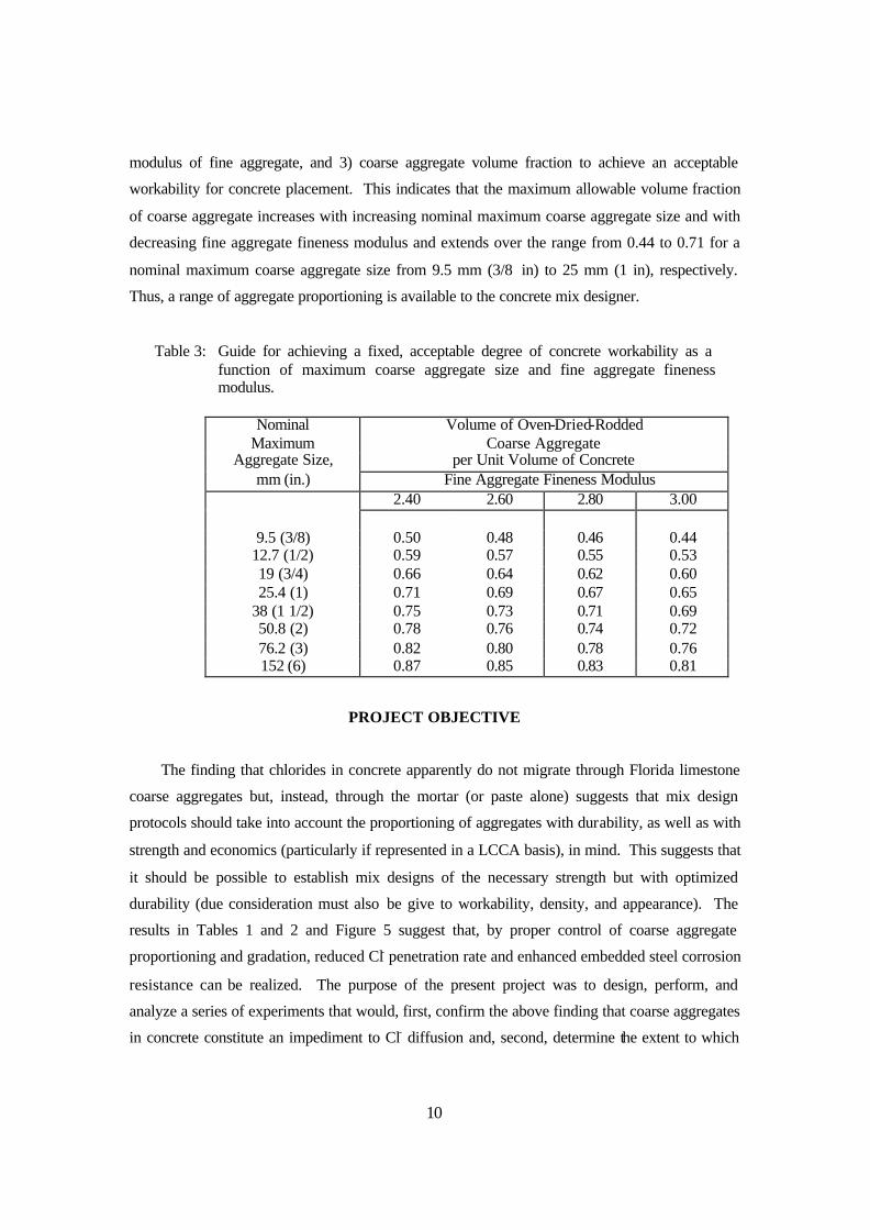
Table 3: Guide for achieving a fixed, acceptable degree of concrete workability as a function of maximum coarse aggregate size and fine aggregate fineness modulus ………………………………….. 10

Table 4: Material properties and mix design parameters for mortar

specimens prepared using low FM silica sand as the FA ……….. 13

Table 5: Material properties and mix design parameters for mortar specimens prepared using high FM silica sand as the FA ……………... 14

Table 6: Comparison of the present “ideal” CA proportioning with ASTM aggregate size #7 ………………………………………………. 15

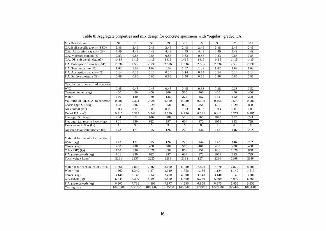
Table 7: Aggregate properties and mix design for concrete specimens

with “ideally” graded CA ……………………………………………… 16

Table 8 Aggregate properties and mix design for concrete specimens with “regular” graded CA ……………………………………………… 17

Table 9: Results of the Iowa Pore Index tests …………………………………… 25 Table 10: Chloride concentration data (kg/m3) for duplicate and

multiple Cl- analyses performed upon samples from Specimens L45-2 and L55-1 ………………………………………….. 27

Table 11: Chloride analysis results for the central and exterior

portion of sections acquired from Specimen L55-2 …………………… 28 Table 12: Chloride concentration data (kg/m3) of samples acquired at

different depths from mortar specimens with low FM silica sand FA …………………………………………………………... 29

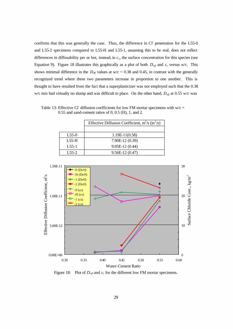
Table 13: Effective Cl- diffusion coefficients for low FM silica sand FA

mortar specimens with w/c = 0.55 and sand-cement ratios of 0, 0.5 (H), 1, and 2 ……………………………………………………… 30

Table 14: Chloride concentration data (kg/m3) for samples acquired at different depths of mortar specimens with high FM silica sand FA ………………………………………………………………… 31

vii

LIST OF TABLES (CONTINUED) page

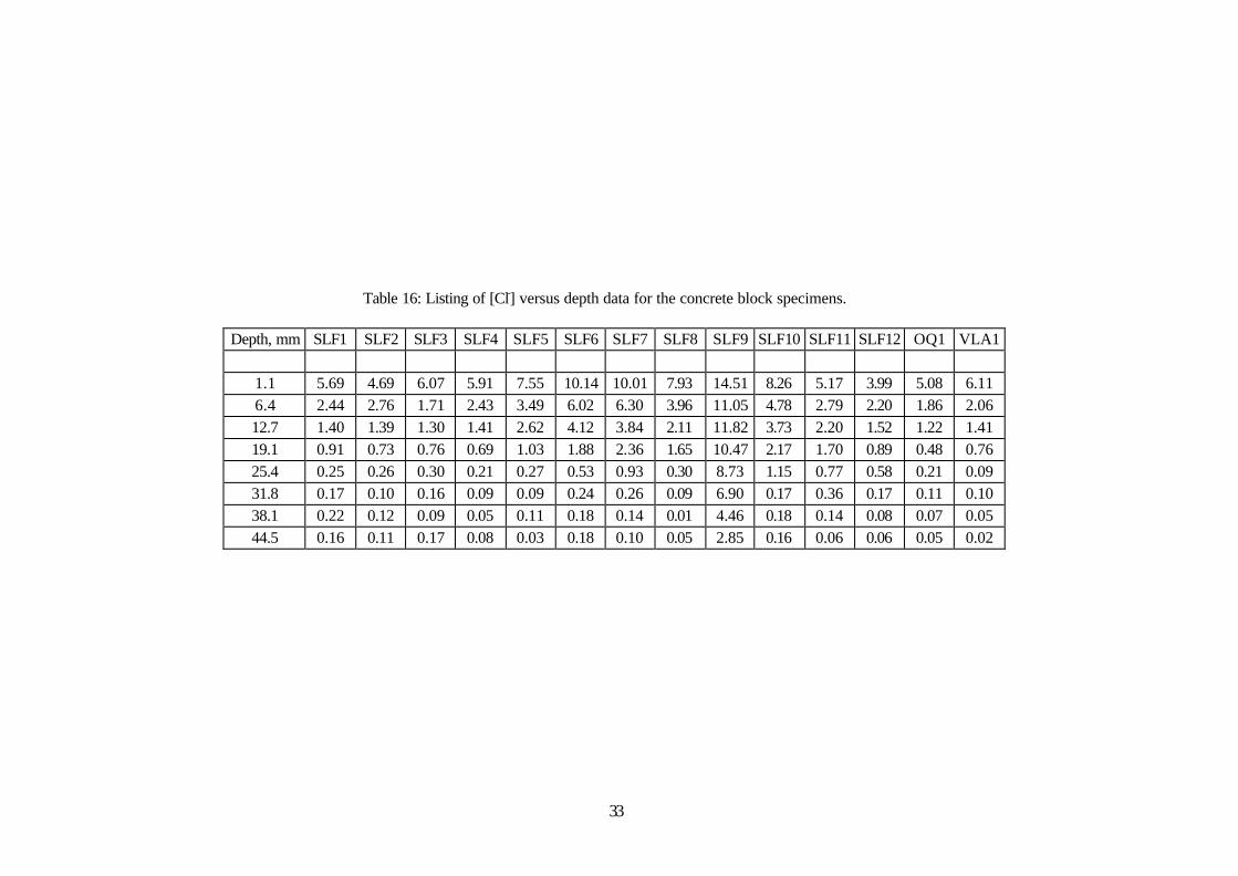
Table 15: Effective diffusion coefficient corresponding to the Cl- profiles in Figure 18 (m2/s (in2/y)) ……………………………………… 32 Table 16: Listing of [Cl-] versus depth data for the concrete block Specimens ……………………………………………………………… 35 Table 17: Effective diffusion coefficient data for the SLF CA mixes

with cement content 400 kg/m3 ………………………………………… 36 Table 18: Effective diffusion coefficient data for specimens of

different cement content ……………………………………………….. 39 Table 19: Effective diffusion coefficient data for specimens with

different coarse aggregate types ……………………………………….. 39 Table 20: Values for Deff for regular and ideal graded mix designs of

three w/c ……………………………………………………………….. 41 Table 21: Comparison of Times-to-Corrosion and required covers based

upon Deff results for the ideal and regular graded coarse aggregates ….. 42

viii

LIST OF FIGURES page

Figure 1: Schematic illustration of sea water migration and Cl- accumulation within a marine piping ………………………………… 4 Figure 2: Photograph of a cracked and spalled marine bridge piling …………… 4 Figure 3: Schematic illustration of the various steps in deterioration of reinforced concrete due to chloride induced corrosion ……………. 5 Figure 4: Schematic illustration of life cycle cost ……………………………… 6 Figure 5: Chloride concentration as a function of depth for mortar and coarse aggregate areas of a concrete core ……………………………… 9 Figure 6: Photograph of the three CA types …………………………………… 15 Figure 7: Photograph of mortar specimens under exposure testing …………… 18 Figure 8: Photograph of concrete block specimens under exposure testing …… 18 Figure 9: Grading curve for the high FM silica sand fine aggregate …………... 20 Figure 10: Grading curve for the regular and ideal SLF CA in comparison to the ASTM limits for size number 7 ……………………………….. 21 Figure 11: Plot of cumulative pore surface area versus pore size for samples of each of the three coarse aggregates …………………….... 24 Figure 12: Plot of cumulative pore volume versus pore size for samples of each of the three coarse aggregates ……………………………….. 24 Figure 13: Plot of cumulative pore volume versus pore size for coarse

aggregate samples from the previous study (13) in comparison to the present …………………………………………………………. 25 Figure 14: Results of Cl- analyses performed upon two samples of the same mortar powder acquired from Specimen L45-2 ……………….. 26

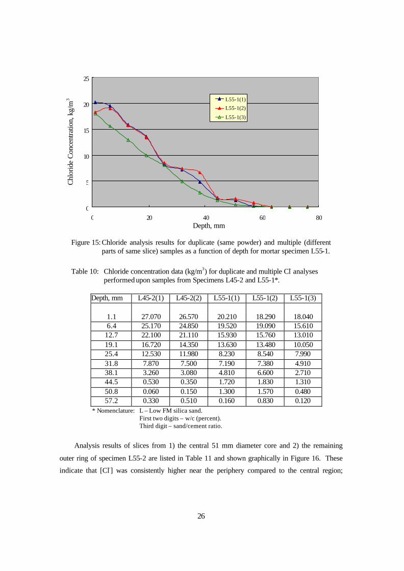
Figure 15: Chloride analysis results for duplicate (same powder) and

multiple (different parts of same slice) samples as a function of depth for mortar specimen L55-1 ………………………. 27

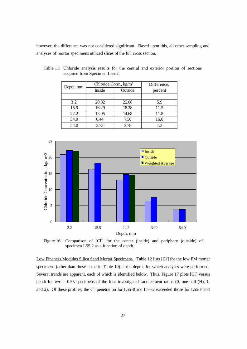
Figure 16 Comparison of [Cl-] for the center (inside) and

periphery (outside) of specimen L55-2 as a function of depth ……… 28 Figure 17: Chloride prof iles versus depth for low FM mortar specimens

with w/c = 0.55 and sand-cement ratios of 0, 0.5 (H), 1, and 2 …….. 29

ix

LIST OF FIGURES (continued) page

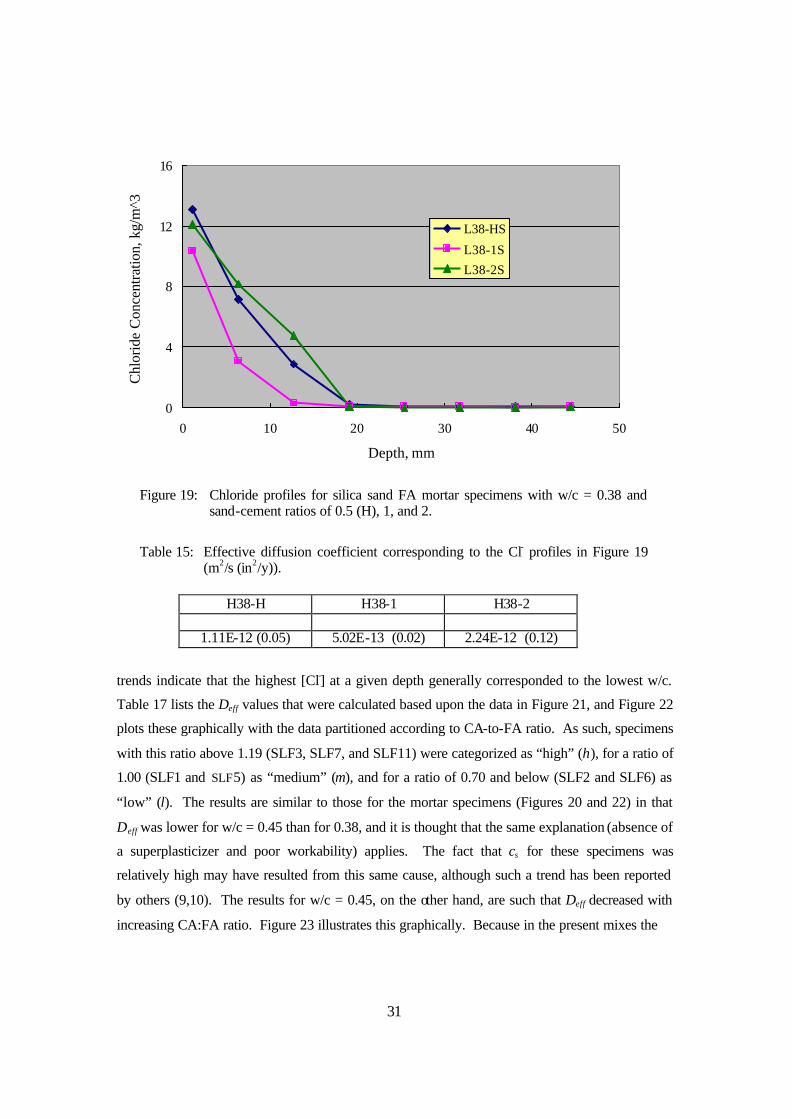
Figure 18: Plot of Deff and cs for the different low FM mortar specimens ……… 30 Figure 19: Chloride profiles for silica sand FA mortar specimens

with w/c = 0.38 and sand-cement ratios of 0.5 (H), 1, and 2 ……….. 32 Figure 20: Plot of Deff and cs as a function of w/c for the different silica sand FA mortar specimens ……………………………………. 33

Figure 21: Chloride profiles for “regular” (as-received) SLF coarse aggregate concrete specimens ………………………………………. 36

Figure 22: Effective diffusion coefficient as a function of w/c according

to high (h), medium (m), and low (l) CA to FA ratios ……………… 37 Figure 23: Plot of Deff versus volume fraction CA for concrete

specimens with w/c = 0.45 ………………………………………….. 37 Figure 24: Comparison of Deff values for all mix designs as a function

of water-cement ratio ………………………………………………… 38 Figure 25: Chloride profiles for specimens SLF1, SLF 9, and

SLF 10 with cement contents of 400, 300, and 500 kg/m3 , respectively ………………………………………………….. 38

Figure 26: Chloride profiles for concrete specimens with each

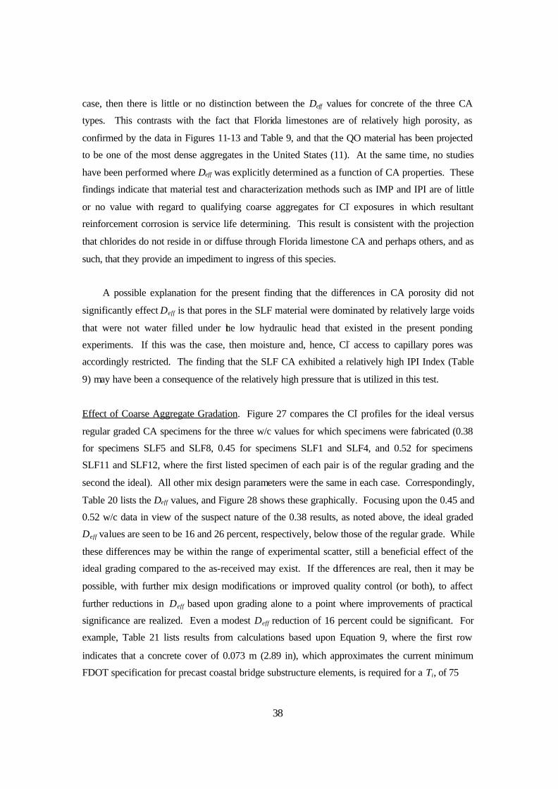
of the three coarse aggregate types …………………………………… 39 Figure 27: Chloride profiles for comparable concrete specimens

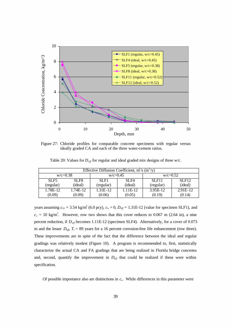
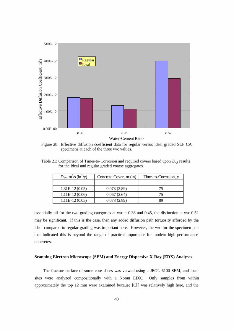
with regular versus ideally graded CA and each of the three water-cement ratios …………………………………………….. 41

Figure 28: Effective diffusion coefficient data for regular versus

ideal graded SLF CA specimens at each of the three w/c values ……. 42 Figure 29: EDX compositional analysis results for samples of the

three aggregate types within a mortar/concrete specimen …………… 43 Figure 30: Compositional analysis for a Ca-rich FA particle in a low FM

mortar specimen …………………………………………………….. 44 Figure 31: EDX compositional analysis results for cement paste areas

of specimens L45-2S (high FM silica sand FA) and L45-2 (low FM silica sand FA) ……………………………………… 44

x

LIST OF FIGURES (continued) page

Figure 32: Scanning electron micrograph (a) of specimen SLF7 showing CA and high FM silica sand particles and cement paste. Locations of EDX scans that traversed the span between the two aggregate particles are also illustrated and (b) analysis results …………………………………… 45

Figure 33: Schematic illustration of the competing affects of sand

content in mortar specimens upon Deff ……………………………….. 47 Figure 34: SEM micrograph of a FA particle and cement matrix f

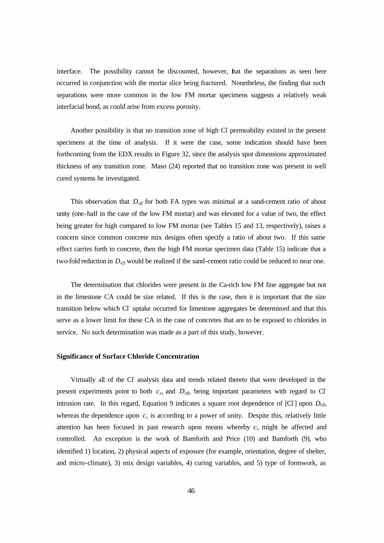
or specimen L45-2 …………………………………………………… 47 Figure 35 Representation of surface Cl- concentration on a cement

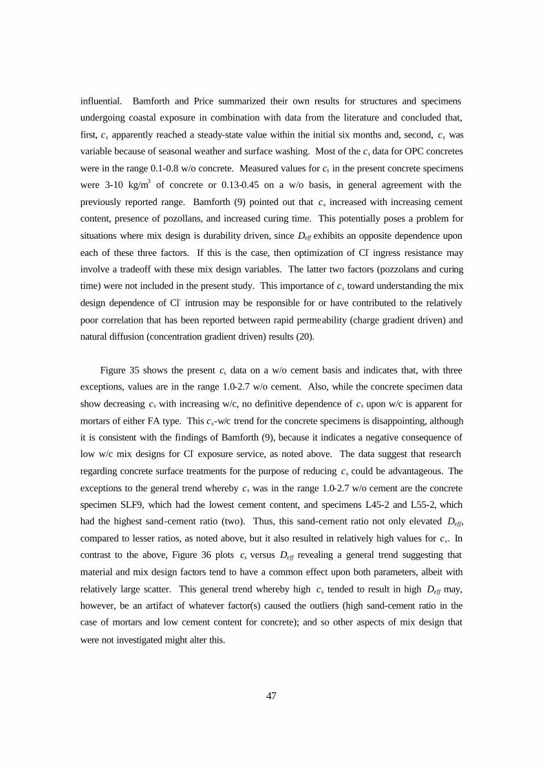
weight basis ………………………………………………………….. 50 Figure 36: Plot of surface chloride concentration versus effective

diffusion coefficient for mortar and concrete specimens …………….. 50

1

INTRODUCTION

Overview of Concrete and Concrete Deterioration Processes

General: While concrete has evolved to become the most widely used structural material in the

world, the fact that its capacity for plastic deformation and, hence, its ability to absorb

mechanically imparted energy is essentially nil imposes major practical service limitations. This

shortcoming is most commonly overcome by incorporation of steel reinforcement into those

locations in the concrete where tensile stresses are anticipated. Consequently, concerns regarding

performance must not only focus upon properties of the concrete per se but also of the embedded

steel and, in addition, the manner in which these two components interact. In this regard, steel

and concrete are in most aspects mutually compatible, as exemplified by the fact that the

coefficient of thermal expansion for each is approximately the same. Also, while boldly exposed

steel corrodes actively in most natural environments at a rate that requires use of extrinsic

corrosion control measures (for example, protective coatings for atmospheric exposures and

cathodic protection in submerged and buried situations), the relatively high pH of concrete pore

water (pH ≈ 13.0-13.8) promotes formation of a protective passive film such that corrosion rate is

negligible and decades of relatively low maintenance result.

Corrosion Mechanism: Disruption of the passive film upon embedded reinforcement and onset of

active corrosion can arise in conjunction with either of two causes: carbonation or chloride

intrusion (or a combination of the two). In the former case (carbonation), atmospheric carbon

dioxide (CO2) reacts with pore water alkali according to the generalized reaction,

( ) OHCaCOCOOHCa 2322 +→+ , (1

which consumes reserve alkalinity and reduces pore water pH to the 8-9 range, where steel is no

longer passive. For dense, high quality concrete (for example, high cement factor, low water -

cement ratio, and pozzolanic admixture) carbonation rates are typically on the order of one mm

per decade or less; and so loss of passivity from this cause within a normal design life is not

generally a concern. On the other hand, carbonation is often a problem for older structures; first,

because of age per se and, second, because earlier ge neration concretes were typically of

relatively poor quality (greater permeability) than more recent ones.

2

Chlorides, on the other hand, arise in conjunction with deicing activities upon northern

roadways or from coastal exposure. While this species (Cl-) has only a small influence on pore

water pH per se, concentrations as low as 0.6 kg/m3 (1.0 pcy) (concrete weight basis) have been

projected to compromise steel passivity. In actuality, it is probably not the concentration of

chlorides per se that governs loss of passivity but rather the ratio of chlorides to hydroxides

([Cl-]/[OH-]), since the latter species (OH-) acts as an inhibitor. This has been demonstrated by

aqueous solution experiments from which it is apparent that the Cl- threshold for loss of steel

passivity increased with increasing pH (1-6). On this basis, the relative amount of cement in the

concrete mix and cement alkalinity are likely to affect the onset of corrosion. Considerable

research effort has been focused upon identification of a chloride threshold; however, a unique

value for this parameter has remained illusive, presumably because of the role of cement,

concrete mix, environmental, potential, and reinforcement (composition and microstructure)

variables that are influential (7). Because Cl- and not carbonation induced loss of passivity is of

primary concern for bridge structures, subsequent focus in this report is upon this cause of

corrosion alone.

Once steel in concrete becomes active, either in conjunction with chlorides achieving the

threshold concentration or pore solution pH reduction from carbonation at the embedded steel

depth, then the classical anodic iron reaction,

−+ +→ 2eFeFe 2 , (2

and cathodic oxygen reaction,

−− →++ 2OH2eOHO21

22 , (3

occur at an accelerated rate. Despite the normally high alkalinity of concrete, acidification may

occur in the vicinity of anodic sites because of oxygen depletion and hydrolysis of ferrous ions.

Thus,

++ +→+ 2HFe(OH)O2HFe 222 . (4

3

The product H+ may be reduced and, along with O2 reduction at more remote cathodic sites,

further stimulate the anodic process. Irrespective of this, the net reaction is,

22

22 Fe(OH)2OHFeOHO21

Fe →+→++ −+ , (5

and, upon further oxidation,

3222 2Fe(OH)OHO21

2Fe(OH) →++ , (6

with,

O3HOFe2Fe(OH) 2323 +→ , (7

as drying takes place.

Interestingly, corrosion per se is seldom the cause of failure in reinforced concrete

components and structures. This arises because the final corrosion products (either ferric oxide or

hydroxide) have a specific volume that is several times greater than that of the reactant steel; and

their accumulation in the concrete pore space adjacent to anodic sites leads to development of

tensile hoop stresses about the steel which, in combination with the relatively low tensile strength

of concrete (typically 1-2 MPa), ultimately causes cracking and spalling.

Damage of this type has evolved to become a significant concern in the case of coastal

bridge sub-structures in Florida. Figure 1 illustrates the deterioration process schematically

where chlorides accumulate within the submerged zone from inward sea water migration and in

the atmospheric zone as a consequence of capillary flow, splash, and spray. The lack of dissolved

oxygen in the submerged zone precludes Reaction 2, and so corrosion is rarely a problem here.

However, ready availability of both Cl- in the splash zone and of O2 at contiguous, more elevated

locations results in this location (splash zone) being particularly susceptible to corrosion induced

damage. Figure 2 shows a photograph of a marine bridge piling that illustrates this.

4

Figure 1: Schematic illustration of sea water migration and Cl- accumulation within a marine piping.

Figure 2: Photograph of a cracked and spalled marine bridge piling.

Representation of Corrosion Induced Concrete Deterioration. Corrosion induced deterioration of

reinforced concrete can be modeled in terms of three component steps: 1) time for corrosion

initiation, 2) time, subsequent to corrosion initiation, for corrosion propagation (appearance of a

crack on the external concrete surface), and 3) time for surface cracks to develop into spalls that

Concrete

Pile

Zone of Maximum Chlorides

Evaporative Water Loss

Inward and Upward Sea Water Flux

Sea Water

5

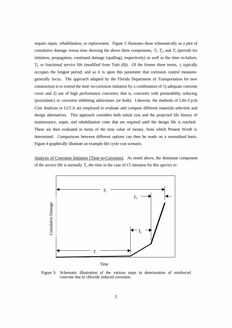
require repair, rehabilitation, or replacement. Figure 3 illustrates these schematically as a plot of

cumulative damage versus time showing the above three components, Ti, Tp, and Td (periods for

initiation, propagation, continued damage (spalling), respectively) as well as the time -to-failure,

Tf, or functional service life (modified from Tutti (8)). Of the former three terms, ti typically

occupies the longest period; and so it is upon this parameter that corrosion control measures

generally focus. The approach adapted by the Florida Department of Transportation for new

construction is to extend the time-to-corrosion initiation by a combination of 1) adequate concrete

cover and 2) use of high performance concretes; that is, concretes with permeability reducing

(pozzolanic) or corrosion inhibiting admixtures (or both). Likewise, the methods of Life-Cycle

Cost Analysis or LCCA are employed to evaluate and compare different materials selection and

design alternatives. This approach considers both initial cost and the projected life history of

maintenance, repair, and rehabilitation costs that are required until the design life is reached.

These are then evaluated in terms of the time value of money, from which Present Worth is

determined. Comparisons between different options can then be made on a normalized basis.

Figure 4 graphically illustrate an example life cycle cost scenario.

Analysis of Corrosion Initiation (Time-to-Corrosion). As noted above, the dominant component

of the service life is normally Ti, the time in the case of Cl- intrusion for this species to

Figure 3: Schematic illustration of the various steps in deterioration of reinforced concrete due to chloride induced corrosion.

Cum

ulat

ive

Dam

age

Time

Ti

Tf

Tp

Td

6

Figure 4: Schematic illustration of life cycle cost.

accumulate at the steel depth to the threshold concentration. The mechanism of this intrusion

invariably involves both capillary suction and diffusion; however, for situations where the depth

to which the former (capillary suction) occurs is relatively shallow compared to the reinforcement

cover, diffusion alone is normally considered. Analysis of the latter (diffusion) is accomplished

in terms of Fick’s second law or,

( ) ( )

∂

∂⋅

∂∂

=∂

∂x

tx,cD

xttx,c

, (8

where c(x,t) is the Cl- concentration at depth x beneath the exposed surface after exposure time t

and D is the diffusion coefficient. As Equation 8 is expressed, D is assumed to be independent of

concentration. The solution in the one-dimensional case is,

⋅−=

−−

tD2

xerf1

ccct)c(x,

os

o , (9

where

co is the initial or background Cl- concentration in the concrete, and

cs is the Cl- concentration on the exposed surface.

Initial Cost

End of Functional Service Life

(Bridge Replacement)

Rehabilitation

Annual Maintenance

Repair

Cos

t

Time

7

Assumptions involved in arriving at this solution are, first, cs and D are constant with time and,

second, the diffusion is “Fickian;” that is, there are no Cl- sources or sinks in the concrete. In

actuality, cs increases with exposure time, although steady-state values generally in the range 0.3-

0.7 (percent of concrete weight) have been projected to result after about six months (9). Factors

that effect cs have been projected to include type of exposure, mix design (cement content, in

particular), and curing conditions (10). Also, the diffusion coefficient that is calculated from

Equation 9 is termed an effective value, Deff, since it is weighted over the relevant exposure

period due, first, to the fact that cs may vary and, second, because of progressive cement

hydration. In addition, chemical and physical Cl- binding invariably occur to some degree such

that the concrete acts as a sink for this species and some fraction is no longer able to diffuse.

By the approach represented by Equation 9, c(x,t), co, and cs are measured experimentally

(normally by wet chemistry analysis) and Deff is calculated based upon knowledge of

reinforcement cover and exposure time. Experimental scatter and error may be minimized by

measuring c(x,t) at multiple depths and employing a curve-fitting algorithm to calculate Deff.

Also, if Deff is known from one sampling set, then cth, the Cl- threshold, can be determined by

measuring c(x,t) at the reinforcement depth (crd) at the time of corrosion initiation and solving

Equation 9 recognizing that for this situation, crd ≈ cth. In any case, the parameters that affect Cl-

intrusion rate are cs, and Deff, where the former is exposure dependent and the latter a material

property (actually, cs is also sensitive to material composition and microstructure and Deff is

affected by exposure conditions (relative humidity and time-of-wetness, for example).

The approach of employing pozzolanic and corrosion inhibiting admixtures that has been

adapted by the FDOT for enhancing concrete durability, as noted above, can be related to and

interpreted in terms of Equation 9. In this regard, Ca(NO2)2, in effect, increases cth, whereas

pozzolans (fly ash, silica fume, and blast furnace slag) reduce Deff. Surface [Cl-] may also be

affected.

PROJECT BACKGROUND

Chloride Distribution in Concrete

Results of a preliminary investigation in which the distribution of Cl- in and migration

through concrete cores from several bridges, including the Long Key Bridge in District 6, were

8

measured serve as the basis for the present research project. In this case, the core was acquired

from the pile cap (inverted) which was about one m above mean high tide. The analyses involved

two procedures; first, wet chemistry analysis of 1) micro-drilled powder and 2) chipped particles,

with the product being acquired from separate coarse aggregate and cement mortar areas and,

second, energy dispersive x-ray analysis (EDX), also upon individual coarse aggregate and

mortar areas. In both cases, the sample areas were on a fractured surface of the core at a given

depth below the exposed surface. EDX analyses were also performed as a function of depth

relative to this exposed surface. Table 1 presents the results from the wet chemistry analyses and

Table 2 for the EDX for the case of analyses at a particular depth. These indicate that the mortar-

to-aggregate chloride concentration ratio in the former case (wet chemistry analysis) was 9:1 and

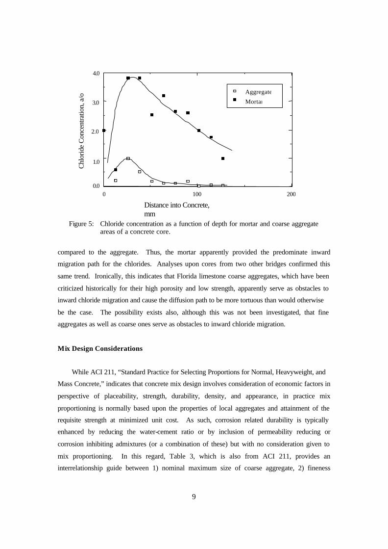
in the latter (EDX analyses) 9.8. Figure 5, on the other hand, plots chloride concentration, [Cl-],

versus distance into the concrete beneath the exposed surface, as determined by EDX. This also

indicates that, for any given depth, approximately ten times more chloride existed in the mortar

Table 1: Chloride analysis results for mortar and aggregate samples acquired from a concrete core as determined by wet chemistry.

Location Sampling Technique Chloride Conc.,* pcy (ppm) Mortar Drilling 7,055 (23.5) Aggregate Drilling 781 (2.6) Mortar Chipping 5,733 (19.1) Aggregate Chipping 634 (2.1) *Acid soluble determination. Table 2: Chloride analysis results for mortar and aggregate areas of a concrete core

as determined by energy dispersive x-ray analysis.

Sample Site Location Chloride Designation Type Concentration, a/o* 1 Aggregate 0.13 2 Aggregate 0 3 Aggregate 0 4 Aggregate 0.41 5 Aggregate 0.61 6 Paste 1.72 7 Paste 2.78 *a/o Atomic percent.

9

Figure 5: Chloride concentration as a function of depth for mortar and coarse aggregate

areas of a concrete core.

compared to the aggregate. Thus, the mortar apparently provided the predominate inward

migration path for the chlorides. Analyses upon cores from two other bridges confirmed this

same trend. Ironically, this indicates that Florida limestone coarse aggregates, which have been

criticized historically for their high porosity and low strength, apparently serve as obstacles to

inward chloride migration and cause the diffusion path to be more tortuous than would otherwise

be the case. The possibility exists also, although this was not been investigated, that fine

aggregates as well as coarse ones serve as obstacles to inward chloride migration.

Mix Design Considerations

While ACI 211, “Standard Practice for Selecting Proportions for Normal, Heavyweight, and

Mass Concrete,” indicates that concrete mix design involves consideration of economic factors in

perspective of placeability, strength, durability, density, and appearance, in practice mix

proportioning is normally based upon the properties of local aggregates and attainment of the

requisite strength at minimized unit cost. As such, corrosion related durability is typically

enhanced by reducing the water-cement ratio or by inclusion of permeability reducing or

corrosion inhibiting admixtures (or a combination of these) but with no consideration given to

mix proportioning. In this regard, Table 3, which is also from ACI 211, provides an

interrelationship guide between 1) nominal maximum size of coarse aggregate, 2) fineness

200 100 0 0.0

1.0

2.0

3.0

4.0

Aggregate

Mortar

Distance into Concrete, mm

Chl

orid

e C

once

ntra

tion,

a/o

10

modulus of fine aggregate, and 3) coarse aggregate volume fraction to achieve an acceptable

workability for concrete placement. This indicates that the maximum allowable volume fraction

of coarse aggregate increases with increasing nominal maximum coarse aggregate size and with

decreasing fine aggregate fineness modulus and extends over the range from 0.44 to 0.71 for a

nominal maximum coarse aggregate size from 9.5 mm (3/8 in) to 25 mm (1 in), respectively.

Thus, a range of aggregate proportioning is available to the concrete mix designer.

Table 3: Guide for achieving a fixed, acceptable degree of concrete workability as a function of maximum coarse aggregate size and fine aggregate fineness modulus.

Nominal

Maximum Volume of Oven-Dried-Rodded

Coarse Aggregate Aggregate Size, per Unit Volume of Concrete mm (in.) Fine Aggregate Fineness Modulus 2.40 2.60 2.80 3.00 9.5 (3/8) 0.50 0.48 0.46 0.44 12.7 (1/2) 0.59 0.57 0.55 0.53 19 (3/4) 0.66 0.64 0.62 0.60 25.4 (1) 0.71 0.69 0.67 0.65 38 (1 1/2) 0.75 0.73 0.71 0.69 50.8 (2) 0.78 0.76 0.74 0.72 76.2 (3) 0.82 0.80 0.78 0.76 152 (6) 0.87 0.85 0.83 0.81

PROJECT OBJECTIVE

The finding that chlorides in concrete apparently do not migrate through Florida limestone

coarse aggregates but, instead, through the mortar (or paste alone) suggests that mix design

protocols should take into account the proportioning of aggregates with durability, as well as with

strength and economics (particularly if represented in a LCCA basis), in mind. This suggests that

it should be possible to establish mix designs of the necessary strength but with optimized

durability (due consideration must also be give to workability, density, and appearance). The

results in Tables 1 and 2 and Figure 5 suggest that, by proper control of coarse aggregate

proportioning and gradation, reduced Cl- penetration rate and enhanced embedded steel corrosion

resistance can be realized. The purpose of the present project was to design, perform, and

analyze a series of experiments that would, first, confirm the above finding that coarse aggregates

in concrete constitute an impediment to Cl- diffusion and, second, determine the extent to which

11

this phenomenon, if confirmed, can be employed in concrete mix design to improve resistance to

reinforcement corrosion.

EXPERIMENTAL PROCEDURE

Mortar Specimens

Non-reinforced cylindrical mortar specimens 152 mm high by 76 mm in diameter of three

different water-to-cement ratios, w/c, (0.38, 0.45, and 0.55) with either “low” or “high” fineness

modulus (FM) silica sand fine aggregate (FA), and Type II cement were cast. Both sand types

were obtained bagged from a local retail supplier. For each w/c ratio, a sand-to-cement ratio of 0,

0.5, 1.0, and 2.0 was employed for a total of 24 different mix designs. Table 4 shows the mix

design parameters for the low FM fine aggregate cylinders and Table 5 for the high. Three

cylinders of each mix design were cast. Specimens were demolded after one day, placed in a 100

percent relative humidity chamber, and sprayed daily with deionized water during the first week

thereafter. The low FM mortar mix with w/c = 0.38 and sand-cement ratio two was too stiff to

place, and the paste only (no FA) with w/c = 0.38 and 0.45 developed cracks during curing and

were not exposed.

Concrete Specimens

Non-reinforced concrete block specimens 12.7 cm wide by 12.7 cm high by 20 cm long

were cast using ASTM Type II cement, silica sand with fineness modulus 2.94 (same material as

for the mortar specimens in Table 4), and coarse aggregate (CA) from each of three different

sources. These were Southdown porous limestone (Florida), Vulcan dense limestone (Alabama),

and Sidley quartz (Ohio); and are subsequently identified as SLF, VLA, and QO, respectively. It

was intended that these represent a relatively broad range of what is commercially available,

where the first (SLF) should be typical of what is employed in Florida, the second (VLA) being a

more dense material that may be employed in the Florida panhandle region, and the third (QO)

representing an extreme with regard to denseness and impermeability (11). In each case, the

coarse aggregate was obtained directly from the company in 55 gallon steel drums. Figure 6

shows a photograph of each of these three materials. Samples of each CA were characterized

12

Table 4: Material properties and mix design parameters for mortar specimens prepared using low FM silica sand as the FA.

Bulk specific gravity (SSD) 2.56 Total moisture (%) 9.65 Absorption capacity (%) 2.15 Surface moisture (%) 7.5 Fineness modules 2.47 Designation L38-2 L38-1 L38-H L38-0 L45-2 L45-1 L45-H L45-0 L55-2 L55-1 L55-H L55-0 w/c 0.38 0.38 0.38 0.38 0.45 0.45 0.45 0.45 0.55 0.55 0.55 0.55 Water (kg) 152 152 152 152 180 180 180 180 220 220 220 220 Cement (kg) 400 400 400 400 400 400 400 400 400 400 400 400 Air (%) 1 1 1 1 1 1 1 1 1 1 1 1 Sand/cement ratio 2.0 1.0 0.5 0.0 2.0 1.0 0.5 0.0 2.0 1.0 0.5 0.0 Masonry F.A SSD (kg) 800 400 200 0 800 400 200 0 800 400 200 0 Total Volume (m3) 0.595 0.437 0.358 0.279 0.623 0.465 0.386 0.307 0.663 0.505 0.426 0.347 Quantity for one m3 Water (kg) 256 348 425 545 289 387 466 586 332 436 517 634 Cement (kg) 673 916 1118 1434 642 861 1037 1303 604 792 939 1153 Fine aggr, SSD (kg) 1345 916 559 0 1285 861 518 0 1207 792 470 0 Fine aggr. wet (kg) 1446 984 601 0 1381 925 557 0 1298 852 505 0 Actual water 155 279 383 545 193 323 428 586 241 376 481 634 Total (kg/m3) 2274 2180 2101 1979 2216 2108 2021 1889 2143 2021 1925 1787 Vol of 3 cylinders +10% =2.30 liters Actual Mix Water (g) 424.1* 640.3 906.3* 1248.9 441.8 739.8 1006.9* 1344.1 553.5 862.8 1127.6* 1453.4 Cement (g) 1542.1 2099.2 2562.1 3286.7 1472.7 1972.8 2376.2 2986.9 1383.8 1816.4 2153.0 2642.6 Fine aggr. wet (g) 3246.1* 2256.7 1348.3* 0.0 3166.4 2120.7 1250.5* 0.0 2975.2 1952.7 1133* 0.0 Cast Date 07/13/00 07/14/00 07/13/00 07/11/00 07/14/00 07/14/00 07/13/00 07/11/00 07/11/00 07/14/00 07/13/00 07/11/00

* Mix design modified according to a FA surface moisture of 7.4.

13

using the Iowa Pore Index test and mercury porosimetry, the former being performed by the Iowa

DOT and the latter by Micromeritics, Inc. of Norcross, GA.

Table 5: Material properties and mix design parameters for mortar specimens prepared using high FM silica sand as the FA.

Bulk specific gravity (SSD) 2.600 2.536 2.536 2.536 2.536 Total moisture (%) 2.00 1.92 1.92 1.92 1.92 Absorption capacity(%) 0.14 Surface moisture (%) 1.86 1.92 1.92 1.92 1.92 Fineness modules 2.94 Designation L38-2S L38-1S L38-HS L45-2S L55-2S w/c 0.38 0.38 0.38 0.45 0.55 Water (kg) 152 152 152 180 220 Cement (Kg) 400 400 400 400 400 Air (%) 1 1 1 1 1 Sand/cement ratio 2.0 1.0 0.5 2.0 2.0 Masonry F.A SSD (kg) 800 400 200 800 800 Total Volume (m3) 0.590 0.438 0.359 0.626 0.666 Quantity for 1m3 Water (kg) 258 347 424 288 331 Cement (kg) 678 913 1115 639 601 Masonry F.A SSD (kg) 1356 913 558 1279 1202 Masonry F.A wet (kg) 1382 930 568 1303 1225 Actual water 233 329 413 263 307 Total (kg/m3) 2292 2172 2097 2206 2133 Vol of 3 cylinders +10% (l) 2.3 Actual Mix Water (g) 697.5 760.3 952.0 609.4 711.0 Cement (g) 2034.7 2099.1 2565.3 1470.6 1382.2 Masonry F.A wet (g) 4145.2 2136.4 1305.5 2993.5 2813.6 Cast Date 01/06/01 01/11/01 01/11/01 01/11/01 01/11/01

A portion of the as-received CA from each source was partitioned according to material

retained upon individual sieve sizes 19.1 mm (3/4 in.), 12.7 mm (1/2 in.), 9.5 mm (3/8 in.), 4.75

mm (No. 4), and 2.36 (No. 8). The CA was then re-proportioned as indicated by Table 6 to

achieve conformity with standard #7 CA (12). The resultant CA was termed “ideal” and was

employed in casting some of the concrete specimens. The remainder of the specimens were cast

using the as-received SLF CA (termed “regular”), subject to the material having passed a 12.7

14

Figure 6: Photograph of the three CA types.

Table 6: Comparison of the present “ideal” CA proportioning with ASTM aggregate size #7.

AASHTO #7, percent

Present Proportioning, percent

Pass 19 mm but retained on 12.7 mm 0-10 10

Pass 12.7 mm but retained on 9.5 mm 20-60 35

Pass 9.5 mm but retained on 4.75 mm (No. 4) 25-70 47

Pass 4.75 mm but retained on 2.36 mm (No. 8) 0-15 8 Retained on 2.36 mm 0-5 0

mm sieve. In addition to CA grading, mix design variables were 1) w/c (0.38, 0.45, and 0.52), 2)

cement content (300, 400, and 500 kg/m3), FA volume ratio (0.236 to 0.411), and 3) CA volume

ratio (0.580 (normal), 0.464 (low), and 0.696 (high)). Table 7 gives the mix design for the

“ideal” CA and Table 8 for the “regular.” The proportioning of the high FM silica sand was also

determined.

Exposure Testing

Approximately one week prior to the beginning of the exposures, specimens were removed

from the humidity chamber and allowed to dry in laboratory air. An 18 cm by 10 cm plexiglass

bath was then fasten to what had been the bottom 12.7 cm by 20 cm face (formed) of the concrete

SLF QO

15

Table 7: Aggregate properties and mix design for concrete specimens with “ideally” graded CA.

SLF Aggregate Type QO VLA S4 S8 S12 C.A. Bulk specific gravity (SSD) 2.62 2.73 2.45 2.45 2.45 C.A. Absorption capacity (%) 0.27 0.19 4.49 4.49 4.49 C.A. Moisture content (%) 0.05 0.02 0.83 0.83 0.83 C.A. OD Unit Weight (kg/m3) 1462 1491 1415 1415 1415 F.A. Bulk specific gravity (SSD) 2.536 2.536 2.536 2.536 2.536 F.A. Total moisture (%) 1.02 1.02 1.02 1.02 1.02 F.A. Absorption capacity (%) 0.14 0.14 0.14 0.14 0.14 F.A. Surface moisture (%) 0.88 0.88 0.88 0.88 0.88 W/C 0.45 0.45 0.45 0.38 0.52 Cement content (kg) 400 400 400 400 400 Water, kg 180 180 180 152 208 Vol. Ratio of OD C.A 0.58 0.58 0.58 0.58 0.58 Coarse Aggregate SSD (kg) 850 866 858 858 858 Air content (m3) 0.03 0.03 0.03 0.03 0.03 Vol of F.A (m3) 0.338 0.346 0.313 0.341 0.285 Fine aggregate SSD (kg) 858 877 794 865 723 Fine aggregate (as-received--wet) (kg) 866 884 801 872 729 Extra water in F.A (kg) 8 8 7 8 6 Adjusted total water needed (kg) 172 172 173 144 202 Material for one m3 of concrete (kg) water 172 172 173 144 202 cement 400 400 400 400 400 C.A. (SSD) 850 866 858 858 858 F.A. (as-received) 866 884 801 872 729 Total weight (kg/m3) 2289 2323 2231 2274 2188 Material for each batch (kg) water 1.380 1.378 1.362 1.136 1.613 cement 3.200 3.200 3.148 3.148 3.200 C.A. (SSD) 6.802 6.931 6.749 6.749 6.860 F.A. (as-received) 6.928 7.074 6.302 6.866 5.833 Casting date 10/30/00 10/30/00 10/20/00 10/23/00 10/31/00

block specimens and a polyethylene pipe section was similarly attached around the bottom

circumference of the mortar cylinders. These then became the upper face that was ponded during

the exposures. In addition, the circumferential surface of the cylinders and side faces of the

concrete block were coated with epoxy. Ponding commenced for the low FM mortar cylinders on

December 14, 2000 (160-163 days after casting). Exposure of the high FM mortar cylinders

began on June 14, 2001 (154-161 days after casting); and for the concrete blocks, SLF S1-S10 on

16

Table 8: Aggregate properties and mix design for concrete specimens with “regular” graded CA.

Mix Designation S1 S2 S3 S9 S10 S5 S6 S7 S11 C.A. Bulk specific gravity (SSD) 2.45 2.45 2.45 2.45 2.45 2.45 2.45 2.45 2.45 C.A. Absorption capacity (%) 4.49 4.49 4.49 4.49 4.49 4.49 4.49 4.49 4.49 C.A. Moisture content (%) 0.83 0.83 0.83 0.83 0.83 0.83 0.83 0.83 0.83 C.A. OD unit weight (kg/m3) 1415 1415 1415 1415 1415 1415 1415 1415 1415 F.A. Bulk specific gravity (SSD) 2.536 2.536 2.536 2.536 2.536 2.536 2.536 2.536 2.536 F.A. Total moisture (%) 1.02 1.02 1.02 1.02 1.02 1.02 1.02 1.02 1.02 F.A. Absorption capacity (%) 0.14 0.14 0.14 0.14 0.14 0.14 0.14 0.14 0.14 F.A. Surface moisture (%) 0.88 0.88 0.88 0.88 0.88 0.88 0.88 0.88 0.88 Calculation for one m3 of concrete W/C 0.45 0.45 0.45 0.45 0.45 0.38 0.38 0.38 0.52 Cement content (kg) 400 400 400 300 500 400 400 400 400 Water 180 180 180 135 225 152 152 152 208 Vol. ratio of OD C.A. to concrete 0.580 0.464 0.696 0.580 0.580 0.580 0.464 0.696 0.580 Coarse aggr. SSD (kg) 858 686 1029 858 858 858 686 1029 858 Air content (m3) 0.03 0.03 0.03 0.03 0.03 0.03 0.03 0.03 0.03 Vol of F.A. (m3) 0.313 0.383 0.243 0.390 0.236 0.341 0.411 0.271 0.285 Fine aggr. SSD (kg) 794 971 616 988 599 865 1042 687 723 Fine aggr. (as-received-wet) (kg) 801 980 622 997 604 872 1051 693 729 Extra water in F.A (kg) 7 9 5 9 5 8 9 6 6 Adjusted total water needed (kg) 173 171 175 126 220 144 143 146 202 Material for one m3 of concrete Water (kg) 173 171 175 126 220 144 143 146 202 Cement (kg) 400 400 400 300 500 400 400 400 400 C.A. (SSD) (kg) 858 686 1029 858 858 858 686 1029 858 F.A. (as-received) (kg) 801 980 622 997 604 872 1051 693 729 Total weight kg/m3 2231 2237 2225 2281 2182 2274 2280 2268 2188 Material for each batch of 7.87L 7.866 7.866 7.866 8.000 8.000 7.870 7.870 7.870 8.000 Water (kg) 1.362 1.349 1.374 1.010 1.758 1.136 1.124 1.149 1.613 Cement (kg) 3.148 3.148 3.148 2.400 4.000 3.148 3.148 3.148 3.200 C.A. (SSD) (kg) 6.749 5.399 8.099 6.860 6.860 6.749 5.399 8.099 6.860 F.A. (as-received) (kg) 6.302 7.711 4.892 7.977 4.835 6.866 8.275 5.456 5.833 Casting date 10/20/00 10/21/00 10/21/02 10/25/00 10/25/00 10/23/00 10/24/00 10/24/00 10/31/00

17

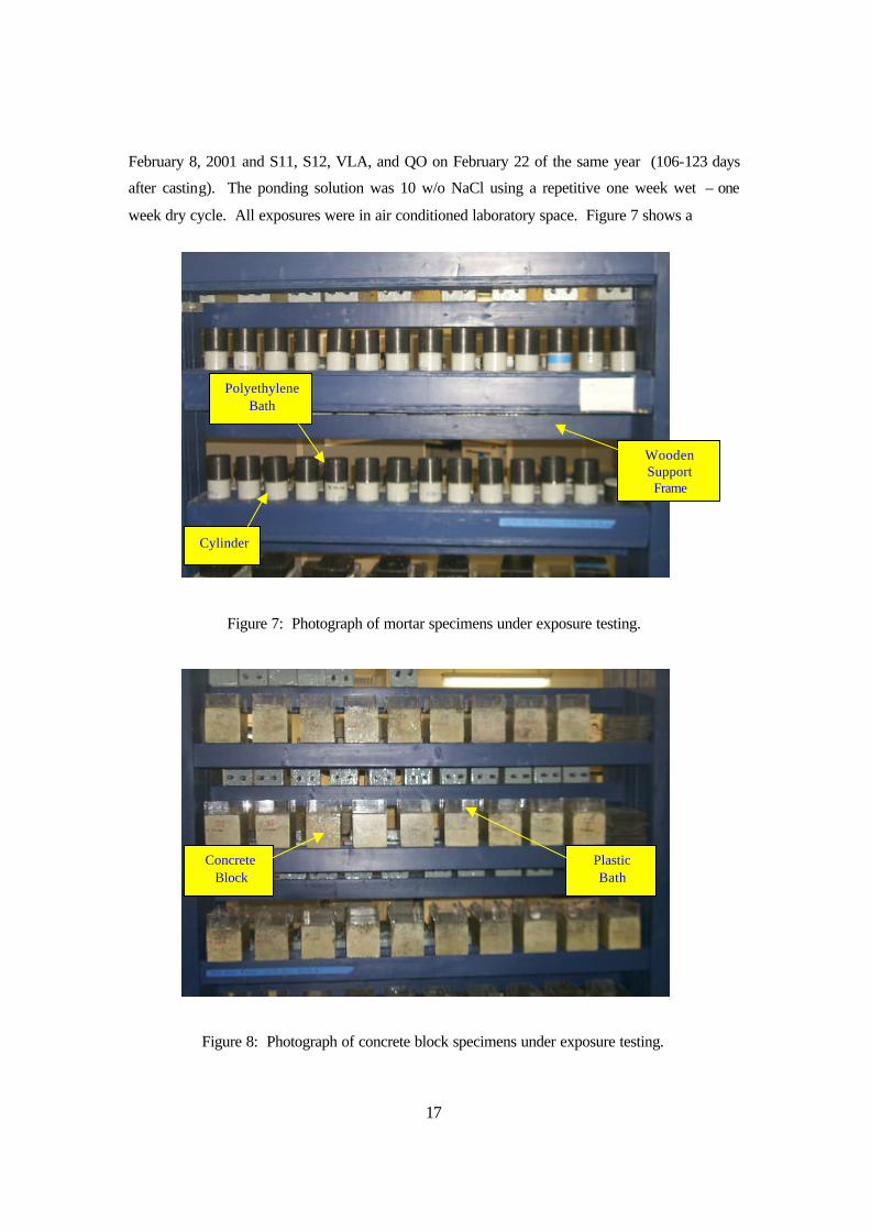
February 8, 2001 and S11, S12, VLA, and QO on February 22 of the same year (106-123 days

after casting). The ponding solution was 10 w/o NaCl using a repetitive one week wet – one

week dry cycle. All exposures were in air conditioned laboratory space. Figure 7 shows a

Figure 7: Photograph of mortar specimens under exposure testing.

Figure 8: Photograph of concrete block specimens under exposure testing.

Cylinder

Polyethylene Bath

Wooden Support Frame

Concrete Block

Plastic Bath

18

photograph of the mortar specimens under test and Figure 8 of the concrete.

Evaluation and Analysis

After the times indicated below, exposure of one of the three specimens of each mix design

was terminated with the other two remaining under test. Exposure of the low FM mortar

specimens was terminated on March 11, 2002 after 452 days exposure, the high FM silica sand

ones on May 7, 2002 after 327 days, and the concrete blocks on April 17, 2002 after 433 days.

Shortly thereafter, the specimens were analyzed for chloride concentration, [Cl-], as a function of

depth beneath the exposed surface. The protocol for the initial mortar specimen that was

analyzed involved extracting a central 51 mm (nominal) diameter core along the cylinder axis

from the exposed face. Both this and the remaining mortar ring were then sliced using a diamond

blade and the slices analyzed. The purpose of this was to determine if [Cl-] exhibited a radial

variation as a consequence of either confinement at the outer surfaces, which should promote

more rapid penetration at the specimen center, or ponding solution seepage at the epoxy-mortar

interface, which would preferentially promote ingress at the periphery. The [Cl-] difference

between the two zones was determined not to be significant, as shown later; and so subsequent

slicing involved the entire cylinder cross section. For the concrete blocks, a 51 mm diameter core

was taken from the center of the ponded area and sliced the same as for the mortar specimens. In

all cases, the slice closest to the exposed surface was three mm thick and subsequent ones six

mm. The slices were broken into fragments, ground to powder using a Scienceware Micro-Mill,

and analyzed for chlorides according to FDOT Test Method FM 5-516 (13). Values for cs and

Deff were then calculated by fitting the [Cl-] versus depth data using a least squares algorithm of

Equation 9 and assuming co = 0. It was considered that the lack of specimen multiplicity was

balanced by the fact that Cl- analyses were performed as a function of depth with the magnitude

of data scatter and material inhomogeniety being indicated by the extent to which the data

conformed to or departed from the general trend.

RESULTS AND DISCUSSION

Silica Sand Sieve Analysis

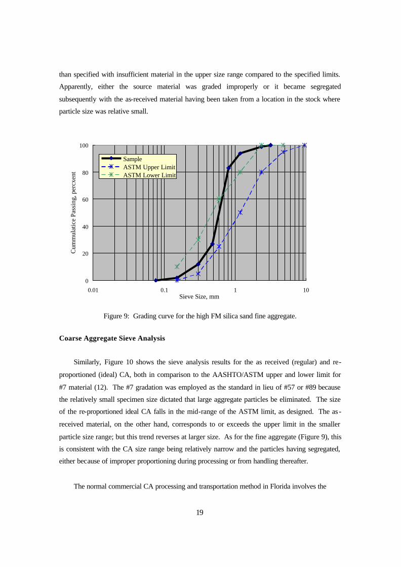
Figure 9 shows the sieve analysis result for the high FM silica sand in comparison to the

AASHTO/ASTM limits (12). This indicates that the particle size distribution was more narrow

19

than specified with insufficient material in the upper size range compared to the specified limits.

Apparently, either the source material was graded improperly or it became segregated

subsequently with the as-received material having been taken from a location in the stock where

particle size was relative small.

0

20

40

60

80

100

0.01 0.1 1 10Sieve Size, mm

Cum

mul

atic

e Pa

ssin

g, p

ercx

ent

SampleASTM Upper LimitASTM Lower Limit

Figure 9: Grading curve for the high FM silica sand fine aggregate.

Coarse Aggregate Sieve Analysis

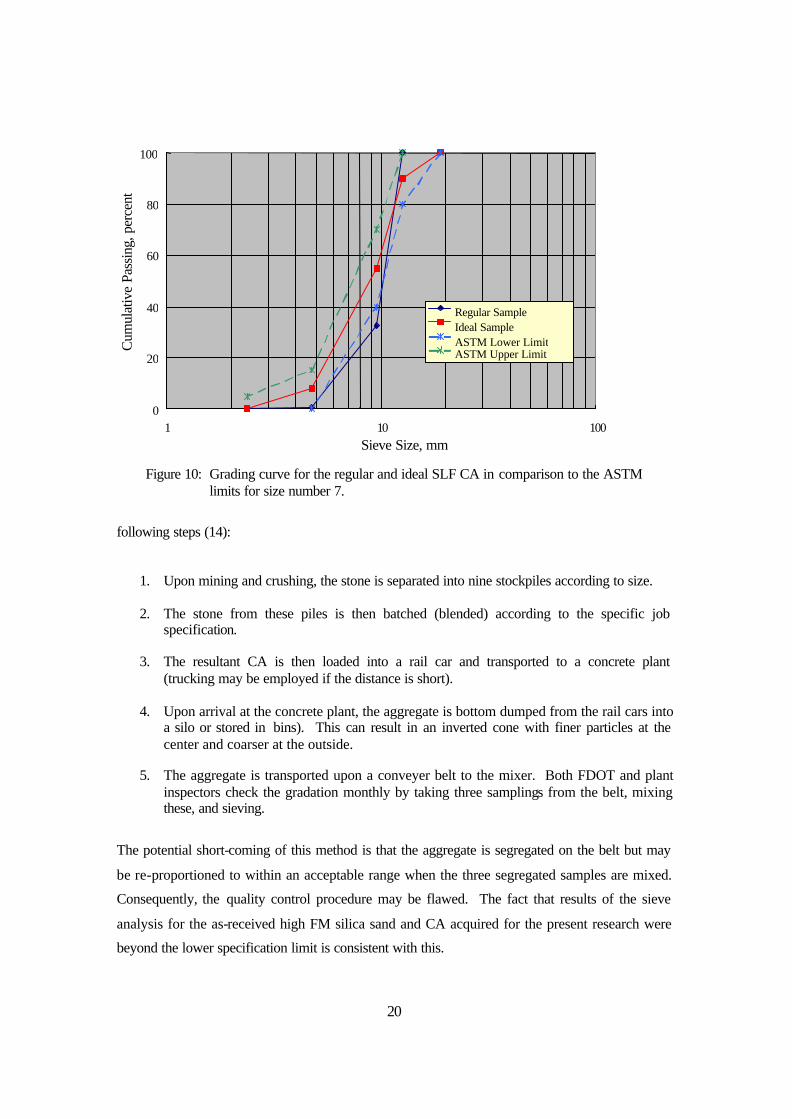
Similarly, Figure 10 shows the sieve analysis results for the as received (regular) and re-

proportioned (ideal) CA, both in comparison to the AASHTO/ASTM upper and lower limit for

#7 material (12). The #7 gradation was employed as the standard in lieu of #57 or #89 because

the relatively small specimen size dictated that large aggregate particles be eliminated. The size

of the re-proportioned ideal CA falls in the mid-range of the ASTM limit, as designed. The as -

received material, on the other hand, corresponds to or exceeds the upper limit in the smaller

particle size range; but this trend reverses at larger size. As for the fine aggregate (Figure 9), this

is consistent with the CA size range being relatively narrow and the particles having segregated,

either because of improper proportioning during processing or from handling thereafter.

The normal commercial CA processing and transportation method in Florida involves the

20

Figure 10: Grading curve for the regular and ideal SLF CA in comparison to the ASTM

limits for size number 7.

following steps (14):

1. Upon mining and crushing, the stone is separated into nine stockpiles according to size. 2. The stone from these piles is then batched (blended) according to the specific job

specification.

3. The resultant CA is then loaded into a rail car and transported to a concrete plant (trucking may be employed if the distance is short).

4. Upon arrival at the concrete plant, the aggregate is bottom dumped from the rail cars into

a silo or stored in bins). This can result in an inverted cone with finer particles at the center and coarser at the outside.

5. The aggregate is transported upon a conveyer belt to the mixer. Both FDOT and plant

inspectors check the gradation monthly by taking three samplings from the belt, mixing these, and sieving.

The potential short-coming of this method is that the aggregate is segregated on the belt but may

be re-proportioned to within an acceptable range when the three segregated samples are mixed.

Consequently, the quality control procedure may be flawed. The fact that results of the sieve

analysis for the as-received high FM silica sand and CA acquired for the present research were

beyond the lower specification limit is consistent with this.

Sieve Size, mm

Cum

ulat

ive

Pass

ing,

per

cent

100

0

20

40

60

80

1 10 100

Regular Sample Ideal Sample ASTM Lower LimitASTM Upper Limit

21

Coarse Aggregate Pore Size Analyses

Concrete permeability, as determined by properties of the cement, FA, and CA components

and the interfacial zone between these, is a fundamental property upon which durability depends.

In the most general sense, the term permeability expresses the relative ease with which a

particular species migrates through the medium of interest in response to a gradient in chemical

potential (most often reflected as a pressure or composition differential). In the latter case

(concentration gradient), the process is termed diffusion; and Equation 9 applies subject to the

transport being Fickian; that is, no sources or sinks for the diffusing species are present within the

medium volume of interest. Porosity, on the other hand, is the void-to-total volume ratio,

normally expressed as a percentage. Porosity and permeability may or may not be interrelated

depending upon the extent of pore interconnectivity. Thus, permeability of a material with a high

density of poorly interconnected pores may be low, while this parameter can be high in the case

of well interconnected pores, even when density for the latter is low.

The problem of characterizing transport through porous materials such as concrete is

complicated by the fact that there are multiple test methods and intrusion mechanisms; for

example, capillary suction, diffusion, and electro-osmosis, each of which can be sensitive to

exposure conditions. In general, the available tests methods provide a parameter that is in some

manner related to permeability, porosity, or to a combination of the two. The situation is

complicated further with attempts to relate a measured parameter that reflects permeability to a

form of durability such as freeze-thaw resistance or, in the present case, Cl- intrusion rate.

Intrusion mercury porosimetry (IMP) and the Iowa Pore Index (IPI) test have been

extensively employed for characterization of coarse aggregates. The former involves recording

the quantity of mercury that becomes injected into an aggregate sample as pressure is

incrementally increased. Because mercury does not wet most materials, including aggregates, the

record reflects progressive uptake by decreasing size pores; and from this, plots of cumulative

uptake versus pore diameter and pore surface area are generated. Thus, the pore size/area

distribution is determined. The IPI, on the other hand, pressurizes a sample using potable water

at 0.24 MPa (35 psi); and the water uptake after one and 14 minutes is recorded. The first of

these parameters (water uptake after one minute) is indicative of water being absorbed into

relatively large pores and, hence, of the volume fraction and interconnectivity of such pores. The

higher this water absorption (number), the easier it is for water to drain from the capillary pores,

22

which is important in the case of freeze-thaw resistance. The second number (14 minute water

uptake) indicates the quantity of water that enters the capillary pores. Durability has been

reported to be relatively low when the second number exceeds 25. However, the Iowa definition

of “durability” presumably pertains to or at least incorporates freeze-thaw resistance, which, of

course, is of little relevance in Florida. Thus, while good freeze -thaw resistance should be

associated with a high first number and low second, it can be reasoned that good resistance to

diffusion of a contaminating species such as chlorides should be realized when both numbers are

low.

Mercury Porosimetry and Iowa Pore Index Test Results

As a part of this research, the three CA types were characterized using both IMP and IPI

tests. Figures 11 and 12 show the IMP results as plots of cumulative pore area and volume versus

pore diameter, respectively, and indicate that the cumulative pore surface area and volume

profiles track each other only in a general sense. Steepness of a particular curve is indicative of

either the pore volume or surface area change within the applicable size range. Comparisons and

conclusions must take into account the logarithmic coordinates. With this in mind, the traces for

the SLF and VLA materials are generally similar, albeit with the cumulative volume and area for

the former exceeding that of the latter by about a factor of two. Pore volume for the QO

aggregate is less than for the SLF and VLA over the entire size range. The relative steepness of

the QO surface area -diameter record compared to the volume-diameter one is indicative of the

smallest pores in this material having a comparatively high surface area. This resulted in the

cumulative surface area of the QO and SLA aggregates being essentially the same, although the

pore volumes of the latter exceeded that of the former by a factor of about four.

A previous study (15) reported IMP determinations performed upon CA samples from six

quarries that are utilized in conjunction with Florida concrete bridge construction. Figure 13

presents the results from these determinations in comparison to the three CAs that were employed

in the present study. This indicates that the three present materials fall within the band

represented by the previous six. Of these, the Calera sample, which is a dense Alabama

limestone and, as such, should be comparable to the VLA, exhibited the least porosity, followed

by the QO material. The SLF, on the other hand, is of comparatively high pore volume.

23

0.001

0.01

0.1

1

10

0.001 0.01 0.1 1 10 100

Pore Diameter, µm

Cum

ulat

ive

Pore

Are

a, m

2/gm VLA

QO

SLF

Figure 11: Plot of cumulative pore surface area versus pore size for samples of each of

the three coarse aggregates.

0.001

0.01

0.1

0.001 0.01 0.1 1 10 100 1000

Pore Diameter, µm

Cum

ulat

ive

Pore

Vol

ume,

ml/g

VLA

QO

SLF

Figure 12: Plot of cumulative pore volume versus pore size for samples of each of the

three coarse aggregates.

24

0.00

0.02

0.04

0.06

0.08

0.10

0.12

0.001 0.01 0.1 1 10 100 1000

Pore Diameter, mm

Cum

ulat

ive

Pore

Vol

ume,

ml

VLAQOSLFCabbage GroveGulf HammockFt. MyersBrooksvilleMiami TarmacCalera

Figure 13: Plot of cumulative pore volume versus pore size for coarse aggregate samples

from the previous study (13) in comparison to the present.

Results from the IPI test (Table 9) indicate that relatively large quantities of water were

absorbed by the SLF aggregate at both measurement increments (one and 14 minutes) compared

to the other two materials, presumably indicating a high pore density/interconnectivity of both

large and capillary pores for the SLF. While this difference is consistent with the IMP results for

the QO aggregate, it is not for the VLA whose record generally tracked that of the SLF. This

may reflect the fact that the two tests are based upon different methods and parameters such that

an expectation of a one-to-one comparison is unrealistic. Also at issue is that IMP utilizes a

single CA particle, whereas the IPI employs a nine kg sample such that statistical variations are

more likely to be an issue for the former than the latter. Clearly, however, both tests indicate that

the SLF aggregate has a more developed pore structure compared to the other two materials.

Table 9: Results of the Iowa Pore Index tests. Aggregate Type Aggregate Designation Iowa Pore Index Southdown Fla. Limestone SLF 208/44 Vulcan Alabama Limestone VLA 0/2 Sidley Ohio Quartz QO 12/2

25

Chloride Analyses

Procedure Qualification. The FDOT Cl- analysis method (13) has been established for several

decades such that sufficient experience has been gained to qualify it as acceptably accurate. With

this in mind, emphasis was placed here upon sample consistency and representativeness. In this

regard, Figure 14 shows [Cl-] as a function of depth for duplicate analyses performed upon

samples of the same powder that was obtained from individual mortar slices of Specimen L45-2.

Here, the average normalized difference between the duplicate samples was 5.4 percent.

Similarly, Figure 15 shows analysis results for specimen L55-1, where data for samples 1 and 2

are for two samples of the same powder (same procedure as for specimen L45-2 (Figure 14)) and

those for sample 3 are for powder from a different portion of the same mortar slice. In the former

case (L55-1(1) and L55-1(2)), the average normalized difference is 7.4 percent (in making both

this and the L45-2 calculation only samples to a depth of 38 mm were considered). For samples

L55-1(2) and L55-1(3), on the other hand, the normalized difference is 28.6 percent. In the case

of duplicate analyses, the difference in results should reflect accuracy of the procedure alone,

whereas for the multiple analyses the difference reflects both this and the heterogeneous nature of

the mortar. Table 10 lists the data in Figures 14 and 15 in tabular form.

0

5

10

15

20

25

30

0 10 20 30 40 50 60 70 80 90

Depth, mm

Chl

orid

e C

once

ntra

tion,

kg/

m^3

L45-2-1st'

L45-2-2nd

Figure 14: Results of Cl- analyses performed upon two samples of the same mortar

powder acquired from Specimen L45-2.

26

Figure 15: Chloride analysis results for duplicate (same powder) and multiple (different

parts of same slice) samples as a function of depth for mortar specimen L55-1.

Table 10: Chloride concentration data (kg/m3) for duplicate and multiple Cl- analyses performed upon samples from Specimens L45-2 and L55-1*.

Depth, mm L45-2(1) L45-2(2) L55-1(1) L55-1(2) L55-1(3) 1.1 27.070 26.570 20.210 18.290 18.040 6.4 25.170 24.850 19.520 19.090 15.610 12.7 22.100 21.110 15.930 15.760 13.010 19.1 16.720 14.350 13.630 13.480 10.050 25.4 12.530 11.980 8.230 8.540 7.990 31.8 7.870 7.500 7.190 7.380 4.910 38.1 3.260 3.080 4.810 6.600 2.710 44.5 0.530 0.350 1.720 1.830 1.310 50.8 0.060 0.150 1.300 1.570 0.480 57.2 0.330 0.510 0.160 0.830 0.120

* Nomenclature: L – Low FM silica sand. First two digits – w/c (percent). Third digit – sand/cement ratio.

Analysis results of slices from 1) the central 51 mm diameter core and 2) the remaining

outer ring of specimen L55-2 are listed in Table 11 and shown graphically in Figure 16. These

indicate that [Cl-] was consistently higher near the periphery compared to the central region;

Depth, mm

Chl

orid

e C

once

ntra

tion,

kg/

m3

0

5

10

15

20

25

0 20 40 60 80

L55-1(1) L55-1(2) L55-1(3)

27

however, the difference was not considered significant. Based upon this, all other sampling and

analyses of mortar specimens utilized slices of the full cross section.

Table 11: Chloride analysis results for the central and exterior portion of sections acquired from Specimen L55-2.

Chloride Conc., kg/m3 Difference,

Depth, mm Inside Outside percent

3.2 20.82 22.08 5.9 15.9 16.29 18.28 11.5 22.2 13.05 14.68 11.8 34.9 6.44 7.56 16.0 54.0 3.73 3.78 1.3

0

5

10

15

20

25

3.2 15.9 22.2 34.9 54.0Depth, mm

Chl

orid

e C

once

ntra

tion,

kg/

m^3

InsideOutsideWeighted Average

Figure 16 Comparison of [Cl-] for the center (inside) and periphery (outside) of

specimen L55-2 as a function of depth.

Low Fineness Modulus Silica Sand Mortar Specimens. Table 12 lists [Cl-] for the low FM mortar

specimens (other than those listed in Table 10) at the depths for which analyses were performed.

Several trends are apparent, each of which is identified below. Thus, Figure 17 plots [Cl-] versus

depth for w/c = 0.55 specimens of the four investigated sand-cement ratios (0, one-half (H), 1,

and 2). Of these profiles, the Cl- penetration for L55-0 and L55-2 exceeded those for L55-H and

28

L55-1 by a depth average of 13 percent. Considering the variation that was apparent in Figure

15, however, this difference may not be statistically significant.

Interestingly, the four profile slopes in Figure 17 are approximately the same, meaning that

the Deff values should also be similar. Table 13 lists Deff for each of these four mix designs and

Table 12: Chloride concentration data (kg/m3) of samples acquired at different depths from mortar specimens with low FM silica sand.

Depth, mm L38-H L38-1 L45-H L45-1 L55-0 L55-H L55-2 1.1 22.910 18.860 17.800 20.950 21.210 19.760 22.460 6.4 15.120 12.980 13.660 13.930 20.780 16.630 21.590 12.7 10.470 9.070 11.270 10.420 17.630 14.240 18.150 19.1 4.230 3.410 6.020 5.850 14.030 9.550 14.960 25.4 0.430 0.280 2.570 2.560 11.110 7.750 11.370 31.8 0.050 0.040 0.520 0.620 8.170 3.930 7.570 38.1 0.000 0.010 0.000 0.060 3.290 1.810 3.800 44.5 0.090 0.000 0.050 0.120 1.820 0.480 1.420 50.8 - 0.000 0.040 0.110 0.290 0.040 0.340 57.2 - 0.000 0.030 0.040 0.260 0.040 0.170

Nomenclature: L – Low FM silica sand. First two digits – w/c (percent). Third digit – sand/cement ratio.

Figure 17: Chloride profiles versus depth for low FM mortar specimens with w/c = 0.55

and sand-cement ratios of 0, 0.5 (H), 1, and 2.

Chl

orid

e C

once

ntra

tion,

kg/

m3

0

5

10

15

20

25

0 10 20 30 40 50 60 70

L55-0 L55-H L55-1 L55-2

29

confirms that this was generally the case. Thus, the difference in Cl- penetration for the L55-0

and L55-2 specimens compared to L55-H and L55-1, assuming this to be real, does not reflect

differences in diffusability per se but, instead, in cs, the surface concentration for this species (see

Equation 9). Figure 18 illustrates this graphically as a plot of both Deff and cs versus w/c. This

shows minimal difference in the Deff values at w/c = 0.38 and 0.45, in contrast with the generally

recognized trend where these two parameters increase in proportion to one another. This is

thought to have resulted from the fact that a superplasticizer was not employed such that the 0.38

w/c mix had virtually no slump and was difficult to place. On the other hand, Deff at 0.55 w/c was

Table 13: Effective Cl- diffusion coefficients for low FM mortar specimens with w/c = 0.55 and sand-cement ratios of 0, 0.5 (H), 1, and 2.

Effective Diffusion Coefficient, m2/s (in2/y) L55-0 1.19E-11(0.58) L55-H 7.90E-12 (0.39) L55-1 9.05E-12 (0.44) L55-2 9.56E-12 (0.47)

Figure 18: Plot of Deff and cs for the different low FM mortar specimens.

0.00E+00

5.00E-12

1.00E-11

1.50E-11

0.30 0.35 0.40 0.45 0.50 0.55 0.60

Water-Cement Ratio

Effe

ctiv

e D

iffus

ion

Coe

ffic

ient

, m2 /s

0

10

20

30

Surf

ace

Chl

orid

e C

onc.

, kg/

m2

-0 (Deff) -H (Deff) -1 (Deff) -2 (Deff)

-0 (cs)-H (cs)-1 (cs)-2 (cs)

30

almost one order of magnitude greater than for 0.45. There is no clear indication that cs was

significantly affected by w/c.

High Fineness Modulus Silica Sand FA Mortar Specimens. Table 14 lists [Cl-] for the mortar

specimens with high FM silica sand fine aggregate at the depths for which samples were

acquired. Of these, Figure 19 plots [Cl-] versus depth for w/c = 0.38 specimens of the three

investigated sand-cement ratios (one-half (H), 1, and 2). Correspondingly, Table 15 lists the Deff

value for these three profiles and indicates that this parameter was lowest for the H38-1 mix

specimen. Figure 20 plots Deff and cs versus w/c for all specimens that were analyzed. Here, the

Deff data for the 0.38 w/c specimens are subject to the same concern expressed above for the low

FM ones. This aside, the limited results indicate the Deff was minimum for the one-to-one sand-

cement mix and was greatest at w/c = 0.55. There are insufficient data to disclose any

dependence of cs upon w/c.

Table 14: Chloride concentration data (kg/m3) for samples acquired at different depths of low FM silica sand mortar specimens.

Depth, mm H38-H H38-1 H38-2 H45-2 H55-2 1.143 13.07 10.36 12.12 16.98 15.72 6.35 7.15 3.06 8.18 8.79 12.90 12.7 2.86 0.31 4.73 5.83 9.05 19.05 0.18 0.09 0.09 1.43 6.30 25.4 0.07 0.08 0.00 0.07 2.74 31.75 0.07 0.08 0.02 0.01 0.63 38.1 0.05 0.04 0.00 0.01 0.41 44.45 0.07 0.06 0.04 0.00 0.31 50.8 - - - - - 57.15 - - - - -

Concrete Block Specimens

Effect of Water-Cement Ratio. Table 16 lists [Cl-] data for all concrete block specimens as a

function of depth below the exposed surface. Correspondingly, Figure 21 plots these data for

specimens with the SLF CA of regular (as-received) grading and a cement content of 400 kg/m3,

with the representation being in terms of both w/c and FA:CA:cement ratio (see Table 7). The

31

0

4

8

12

16

0 10 20 30 40 50

Depth, mm

Chl

orid

e C

once

ntra

tion,

kg/

m^3

L38-HS

L38-1SL38-2S

Figure 19: Chloride profiles for silica sand FA mortar specimens with w/c = 0.38 and

sand-cement ratios of 0.5 (H), 1, and 2.

Table 15: Effective diffusion coefficient corresponding to the Cl- profiles in Figure 19 (m2/s (in2/y)).

H38-H H38-1 H38-2 1.11E-12 (0.05) 5.02E-13 (0.02) 2.24E-12 (0.12)

trends indicate that the highest [Cl-] at a given depth generally corresponded to the lowest w/c.

Table 17 lists the Deff values that were calculated based upon the data in Figure 21, and Figure 22

plots these graphically with the data partitioned according to CA-to-FA ratio. As such, specimens

with this ratio above 1.19 (SLF3, SLF7, and SLF11) were categorized as “high” (h), for a ratio of

1.00 (SLF1 and SLF5) as “medium” (m), and for a ratio of 0.70 and below (SLF2 and SLF6) as

“low” (l). The results are similar to those for the mortar specimens (Figures 20 and 22) in that

Deff was lower for w/c = 0.45 than for 0.38, and it is thought that the same explanation (absence of

a superplasticizer and poor workability) applies. The fact that cs for these specimens was

relatively high may have resulted from this same cause, although such a trend has been reported

by others (9,10). The results for w/c = 0.45, on the other hand, are such that Deff decreased with

increasing CA:FA ratio. Figure 23 illustrates this graphically. Because in the present mixes the

32

Figure 20: Plot of Deff and cs as a function of w/c for the different silica sand FA mortar specimens.

CA:FA ratio was directly proportional to the CA volume fraction, the w/c = 0.45 results are

consistent with the premise that coarse aggregates provide an impediment to Cl- ingress.

Figure 24 plots Deff versus w/c for all mortar specimens and specimens with the SLF CA of

the regular grading. With the reversal of the normal Deff-w/c trend for concrete specimens with

w/c = 0.38 and 0.45 aside, the data generally conform to a common trend of progressively

increasing Deff with increasing w/c. The major exception is SLF9 (w/c = 0.45 and Deff = 1.81E-

11) which had a relatively low cement content (300 kg/m3). Also at issue is one or more of the

seven low FM mortar specimens with w/c of either 0.45 or 0.55. For these cases where Deff was

relatively high, the sand-cement ratio was either zero (paste specimen) or two.

Effect of Cement Content. Figure 25 shows Cl- profiles for specimens SLF9, SLF1, and SLF10

for which the cement contents were 300, 400, and 500 kg/m3 , respectively (w/c ratio was constant

at 0.45). These data indicate that the mix with the lowest cement content clearly exhibited the

highest [Cl-] at a given depth. This was followed by the 500 kg/m3 cement mix, with the 400

kg/m3 one having the lowest Cl- penetration. Table 18 lists the Deff values that correspond to

Water-Cement Ratio

0.00E+00

2.00E-12

4.00E-12

6.00E-12

8.00E-12

1.00E-11

0.30 0.35 0.40 0.45 0.50 0.55 0.60

Effe

ctiv

e D

iffus

ion

Coe

ffic

ient

, m2 /s

0

5

10

15

20

Surf

ace

Chl

orid

e C

onc.

, kg/

m3

-H-1-2-H (cs)-1 (cs)-2 (cs)

33

Table 16: Listing of [Cl-] versus depth data for the concrete block specimens. Depth, mm SLF1 SLF2 SLF3 SLF4 SLF5 SLF6 SLF7 SLF8 SLF9 SLF10 SLF11 SLF12 OQ1 VLA1 1.1 5.69 4.69 6.07 5.91 7.55 10.14 10.01 7.93 14.51 8.26 5.17 3.99 5.08 6.11 6.4 2.44 2.76 1.71 2.43 3.49 6.02 6.30 3.96 11.05 4.78 2.79 2.20 1.86 2.06 12.7 1.40 1.39 1.30 1.41 2.62 4.12 3.84 2.11 11.82 3.73 2.20 1.52 1.22 1.41 19.1 0.91 0.73 0.76 0.69 1.03 1.88 2.36 1.65 10.47 2.17 1.70 0.89 0.48 0.76 25.4 0.25 0.26 0.30 0.21 0.27 0.53 0.93 0.30 8.73 1.15 0.77 0.58 0.21 0.09 31.8 0.17 0.10 0.16 0.09 0.09 0.24 0.26 0.09 6.90 0.17 0.36 0.17 0.11 0.10 38.1 0.22 0.12 0.09 0.05 0.11 0.18 0.14 0.01 4.46 0.18 0.14 0.08 0.07 0.05 44.5 0.16 0.11 0.17 0.08 0.03 0.18 0.10 0.05 2.85 0.16 0.06 0.06 0.05 0.02

34

0

2

4

6

8

10

12

0 10 20 30 40 50

Depth, mm

Chl

orid

e C

once

ntra

tion,

kg/

m^3

SLF1 (w/c=0.45;FA/CA/C=2.00/2.00.100)

SLF2 (w/c=0.45;FA/CA/C=2.45/1.72/1.00)

SLF3 (w/c=0.45;FA/CA/C=1.54/2.57/1.00)

SLF5 (w/c=0.38;FA/CA/C=2.16/2.17.1.00)

SLF6 (w/c=0.38;FA/CA/C=2.60/1.70/1.00)

SLF7 (w/c=0.38(FA/CA/C=1.70/2.60/1.00)

SLF11 (w/c=0.52;FA/CA/C=1.81/2.15/1.00)

Figure 21: Chloride profiles for “regular” (as-received) SLF coarse aggregate concrete

specimens.

Table 17: Effective diffusion coefficient data for the SLF CA mixes with cement content 400 kg/m3.

w/c FA/CA/C Specimen No. Effective Diffusion Coefficient, m2/s (in2/y) 2.16/2.15/1.00 SLF5 1.78E-12 (0.09) 0.38 2.60/1.70/1.00 SLF6 2.50E-12 (0.12) 1.70/2.60/1.00 SLF7 2.81E-12 (0.14) 2.00/2.00/1.00 SLF1 1.31E-12 (0.06) 0.45 2.45/1.72/1.00 SLF2 1.90E-12 (0.09) 1.54/2.57/1.00 SLF3 5.33E-13 (0.03) 0.52 1.81/2.15/1.00 SLF11 3.95E-12 (0.19)

these data and shows that this parameter was lowest for the 400 kg/m3 mix (specimen SLF1),

although the difference between it and the 500 kg/m3 specimen (SLF10) may be within the range

of expected scatter. Again, the variation in cs was predominantly responsible for the differences

in [Cl-] at a given depth.

Effect of Coarse Aggregate Type. Figure 26 presents [Cl-] profiles for specimens with each of

35

Figure 22: Effective diffusion coefficient as a function of w/c according to high (h), medium (m), and low (l) CA to FA ratios.

Figure 23: Plot of Deff versus volume fraction CA for concrete specimens with w/c = 0.45.

0.00E+00

1.00E-12

2.00E-12

3.00E-12

4.00E-12

5.00E-12

0.35 0.40 0.45 0.50 0.55 Water-Cement Ratio

Effe

ctiv

e D

iffus

ion

Coe

ffic

ient

, m2 /s

hm l

0.00E+00

5.00E-13

1.00E-12

1.50E-12

2.00E-12

0.40 0.50 0.60 0.70 0.80

CA Volume Fraction

Effe

ctiv

e D

iffus

ion

Coe

ffic

ient

, m2 /s

36

Figure 24: Comparison of Deff values for all mix designs as a function of water-cement ratio.

0

4

8

12

16

0 10 20 30 40 50

Depth, mm

Chl

orid

e C

once

ntra

tion,

kg/

m^3 SLF1

SLF9

SLF10

Figure 25: Chloride profiles for specimens SLF1, SLF 9, and SLF 10 with cement

contents of 400, 300, and 500 kg/m3, respectively.

0.00E+00

5.00E-12

1.00E-11

1.50E-11

2.00E-11

0.30 0.40 0.50 0.60

Water-Cement Ratio

Effe

ctiv

e D

iffus

ion

Coe

ffic

ient

, m2 /s

Low FM FAHigh FM FAConcrete

37

Table 18: Effective diffusion coefficient data for specimens of different cement content. Specimen No. S9 (300 kg/m3) S1 (400 kg/m3) S10 (500 kg/m3) Deff 1.81E-11 (0.88) 3.34E-12 (0.06) 4.52E-12 (0.17)

0

2

4

6

8

0 10 20 30 40 50Depth, mm

Chl

orid

e C

once

ntra

tion,

kg/

m^3

SLF4

QO1VLA1

Figure 26: Chloride profiles for concrete specimens with each of the three coarse

aggregate types.

the three types of CA, all other mix design factors being the same1. With perhaps the exception

of a lower cs for the QO material, the profiles essentially superimpose. Correspondingly, Table

19 lists the Deff values that were calculated for each of these three specimens and shows that this

parameter was 16 percent higher than for the SLF compared to VLA CA mix and 26 percent

higher than for the QO. Such differences may be within the range of normal scatter. If this is the

Table 19: Effective diffusion coefficient data for specimens with different coarse aggregate types.

Specimen No. SLF4 QO1 VLA1 Deff 1.11E-12 (0.05) 9.28E-13 (0.05) 8.19E-13 (0.04)

1 These three mix designs (S4, VLA, and QO) were based upon ideally graded CA rather than regular (as-received).

38

case, then there is little or no distinction between the Deff values for concrete of the three CA

types. This contrasts with the fact that Florida limestones are of relatively high porosity, as

confirmed by the data in Figures 11-13 and Table 9, and that the QO material has been projected

to be one of the most dense aggregates in the United States (11). At the same time, no studies

have been performed where Deff was explicitly determined as a function of CA properties. These

findings indicate that material test and characterization methods such as IMP and IPI are of little

or no value with regard to qualifying coarse aggregates for Cl- exposures in which resultant

reinforcement corrosion is service life determining. This result is consistent with the projection

that chlorides do not reside in or diffuse through Florida limestone CA and perhaps others, and as

such, that they provide an impediment to ingress of this species.

A possible explanation for the present finding that the differences in CA porosity did not

significantly effect Deff is that pores in the SLF material were dominated by relatively large voids

that were not water filled under the low hydraulic head that existed in the present ponding

experiments. If this was the case, then moisture and, hence, Cl- access to capillary pores was

accordingly restricted. The finding that the SLF CA exhibited a relatively high IPI Index (Table

9) may have been a consequence of the relatively high pressure that is utilized in this test.

Effect of Coarse Aggregate Gradation. Figure 27 compares the Cl- profiles for the ideal versus

regular graded CA specimens for the three w/c values for which specimens were fabricated (0.38

for specimens SLF5 and SLF8, 0.45 for specimens SLF1 and SLF4, and 0.52 for specimens

SLF11 and SLF12, where the first listed specimen of each pair is of the regular grading and the

second the ideal). All other mix design parameters were the same in each case. Correspondingly,

Table 20 lists the Deff values, and Figure 28 shows these graphically. Focusing upon the 0.45 and

0.52 w/c data in view of the suspect nature of the 0.38 results, as noted above, the ideal graded

Deff values are seen to be 16 and 26 percent, respectively, below those of the regular grade. While

these differences may be within the range of experimental scatter, still a beneficial effect of the

ideal grading compared to the as-received may exist. If the differences are real, then it may be

possible, with further mix design modifications or improved quality control (or both), to affect

further reductions in Deff based upon grading alone to a point where improvements of practical

significance are realized. Even a modest Deff reduction of 16 percent could be significant. For

example, Table 21 lists results from calculations based upon Equation 9, where the first row

indicates that a concrete cover of 0.073 m (2.89 in), which approximates the current minimum

FDOT specification for precast coastal bridge substructure elements, is required for a Ti, of 75

39

0

2

4

6

8

10

0 10 20 30 40 50Depth, mm

Chl

orid

e C

once

ntra

tion,

kg/

m^3

SLF1 (regular, w/c=0.45)

SLF4 (ideal, w/c=0.45)SLF5 (regular, w/c=0.38)SLF8 (ideal, w/c=0.38)

SLF11 (regular, w/c=0.52)SLF12 (ideal, w/c=0.52)

Figure 27: Chloride profiles for comparable concrete specimens with regular versus

ideally graded CA and each of the three water-cement ratios.

Table 20: Values for Deff for regular and ideal graded mix designs of three w/c. Effective Diffusion Coefficient, m2/s (in2/y) w/c=0.38 w/c=0.45 w/c=0.52

SLF5

(regular) SLF8 (ideal)

SLF1 (regular)

SLF4 (ideal)

SLF11 (regular)

SLF12 (ideal)

1.78E-12 (0.09)

1.74E-12 (0.09)

1.31E-12 (0.06)

1.11E-12 (0.05)

3.95E-12 (0.19)

2.91E-12 (0.14)

years assuming cth = 3.54 kg/m3 (6.0 pcy), co = 0, Deff = 1.31E-12 (value for specimen SLF1), and

cs = 10 kg/m3. However, row two shows that this cover reduces to 0.067 m (2.64 in), a nine

percent reduction, if Deff becomes 1.11E-12 (specimen SLF4). Alternatively, for a cover of 0.073

m and the lesser Deff, Ti = 89 years for a 16 percent corrosion-free life enhancement (row three).

These improvements are in spite of the fact that the difference between the ideal and regular

gradings was relatively modest (Figure 10). A program is recommended to, first, statistically

characterize the actual CA and FA gradings that are being realized in Florida bridge concretes

and, second, quantify the improvement in Deff that could be realized if these were within

specification.

Of possible importance also are distinctions in cs. While differences in this parameter were

40

Figure 28: Effective diffusion coefficient data for regular versus ideal graded SLF CA specimens at each of the three w/c values.

Table 21: Comparison of Times-to-Corrosion and required covers based upon Deff results for the ideal and regular graded coarse aggregates.

Deff, m

2/s (in2/y) Concrete Cover, m (in) Time-to-Corrosion, y 1.31E-12 (0.05) 0.073 (2.89) 75 1.11E-12 (0.06) 0.067 (2.64) 75 1.11E-12 (0.05) 0.073 (2.89) 89

essentially nil for the two grading categories at w/c = 0.38 and 0.45, the distinction at w/c 0.52

may be significant. If this is the case, then any added diffusion path tortuosity afforded by the

ideal compared to regular grading was important here. However, the w/c for the specimen pair

that indicated this is beyond the range of practical importance for modern high performance

concretes.

Scanning Electron Microscope (SEM) and Energy Dispersive X-Ray (EDX) Analyses

The fracture surface of some core slices was viewed using a JEOL 6100 SEM, and local

sites were analyzed compositionally with a Noran EDX. Only samples from within

approximately the top 12 mm were examined because [Cl-] was relatively high here, and the

0.00E+00

1.00E-12

2.00E-12

3.00E-12

4.00E-12

5.00E-12

0.38 0.45 0.52 Water-Cement Ratio

Effe

ctiv

e D

iffus

ion

Coe

ffic

ient

, m2 /s

Regular Ideal

41

sensitivity/accuracy of EDX at concentrations below approximately one percent, as generally

existed at greater depths, can be poor.

Figure 29 shows the composition for individual particles of each of the three predominant

aggregate types (SLF and high and low FM silica sand). Thus, this CA was comprised

predominantly of Ca with minor amounts of Mg, S, and Fe. Both silica sands, on the other hand,

were mostly Si but with some Ca. Further analysis indicated that approximately 80 percent of the

low FM fine aggregate was silica-rich, presumably as SiO2, and the remainder Ca-rich (CaCO3).

Composition of the silica sand in both FA types (high and low FM) was essentially the same.

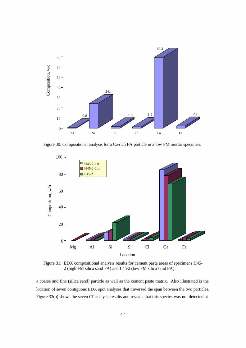
Figure 30 shows the analysis results for a low FM particle that was Ca rich, presumably a

limestone fine. Note, however, that while no Cl- was detected for the CA or high FM silica sand,

including Si-rich FA in the exposed masonry sand specimens, this species was present in the Ca

rich FA. This trend, where Cl- was present in the Ca rich FA particles, may have been

responsible for the relatively high cs of this species exhibited by mortar specimens that utilized

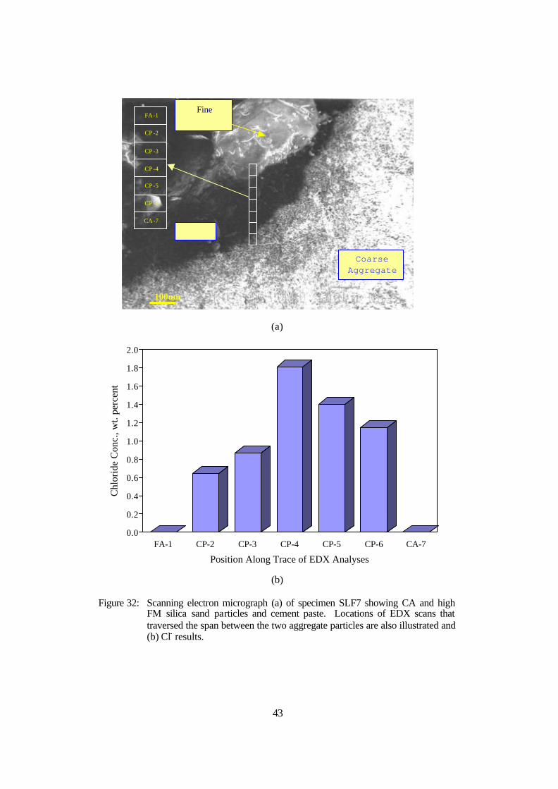
this material. Likewise, Figure 31 shows analysis results for the paste area of specimens of both

FA types. This indicates Ca, and to a lesser extent Si, were the major components here with

minor concentrations of Mg, Al, Fe, and S, as well as Cl-.

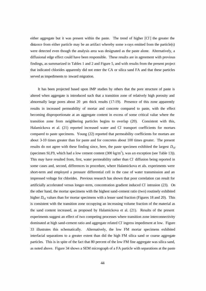
Figure 32(a) is an electron micrograph of a fracture face from specimen SLF7 showing both

0

20

40

60

80

100

Com

posi

tion,

wt.

perc

ent

Mg Al Si S Cl Ca Fe

Element

Coarse Aggregate

High FM Fine Aggr.Low FM Fine Aggr.

Figure 29: EDX compositional analysis results for samples of the three aggregate types

within a mortar/concrete specimen.

42

Figure 30: Compositional analysis for a Ca-rich FA particle in a low FM mortar specimen.

Figure 31: EDX compositional analysis results for cement paste areas of specimens H45-2 (high FM silica sand FA) and L45-2 (low FM silica sand FA).

a coarse and fine (silica sand) particle as well as the cement paste matrix. Also illustrated is the

location of seven contiguous EDX spot analyses that traversed the span between the two particles.

Figure 32(b) shows the seven Cl- analysis results and reveals that this species was not detected at

Com

posi

tion,

w/o

0.8

24.4

1.8 1.5

69.3

2.2

0

10

20

30

40

50

60

70

Al Si S Cl Ca Fe

Com

posi

tion,

w/o

0

20

40

60

80

100

Mg Al Si S Cl Ca Fe

Location

H45-2-1st H45-2-2nd L45-2

43

(a)

0.0

0.2

0.4

0.6

0.8

1.0

1.2

1.4

1.6

1.8

2.0

Chl

orid

e C

onc.

, wt.

perc

ent

FA-1 CP-2 CP-3 CP-4 CP-5 CP-6 CA-7

Position Along Trace of EDX Analyses

(b)

Figure 32: Scanning electron micrograph (a) of specimen SLF7 showing CA and high FM silica sand particles and cement paste. Locations of EDX scans that traversed the span between the two aggregate particles are also illustrated and (b) Cl- results.

FA-1

CP -2

CP -3

CP -4

CP -5

CP -6

CA-7

Fine

Aggregat

Coarse Aggregate

100um

Paste

44

either aggregate but it was present within the paste. The trend of higher [Cl-] the greater the

distance from either particle may be an artifact whereby some x-rays emitted from the particle(s)

were detected even though the analysis area was designated as the paste alone. Alternatively, a

diffusional edge effect could have been responsible. These results are in agreement with previous

findings, as summarized in Tables 1 and 2 and Figure 5, and with results from the present project

that indicated chlorides apparently did not enter the CA or silica sand FA and that these particles

served as impediments to inward migration.

It has been projected based upon IMP studies by others that the pore structure of paste is

altered when aggregate is introduced such that a transition zone of relatively high porosity and

abnormally large pores about 20 µm thick results (17-19). Presence of this zone apparently

results in increased permeability of mortar and concrete compared to paste, with the effect

becoming disproportionate at an aggregate content in excess of some critical value where the

transition zone from neighboring particles begins to overlap (20). Consistent with this,

Halamickova et al. (21) reported increased water and Cl- transport coefficients for mortars

compared to paste specimens. Young (22) reported that permeability coefficients for mortars are

about 3-10 times greater than for paste and for concretes about 100 times greater. The present

results do not agree with these finding since, here, the paste specimen exhibited the largest Deff

(specimen SLF9, which had a low cement content (300 kg/m3), was an exception (see Table 13)).

This may have resulted from, first, water permeability rather than Cl- diffusion being reported in

some cases and, second, differences in procedure, where Halamickova et als. experiments were

short-term and employed a pressure differential cell in the case of water transmission and an

impressed voltage for chlorides. Previous research has shown that poor correlation can result for

artificially accelerated versus longer-term, concentration gradient induced Cl- intrusion (23). On

the other hand, the mortar specimens with the highest sand-cement ratio (two) routinely exhibited

higher Deff values than for mortar specimens with a lesser sand fraction (Figures 18 and 20). This

is consistent with the transition zone occupying an increasing volume fraction of the material as

the sand content increased, as proposed by Halamickova et al. (21). Results of the present

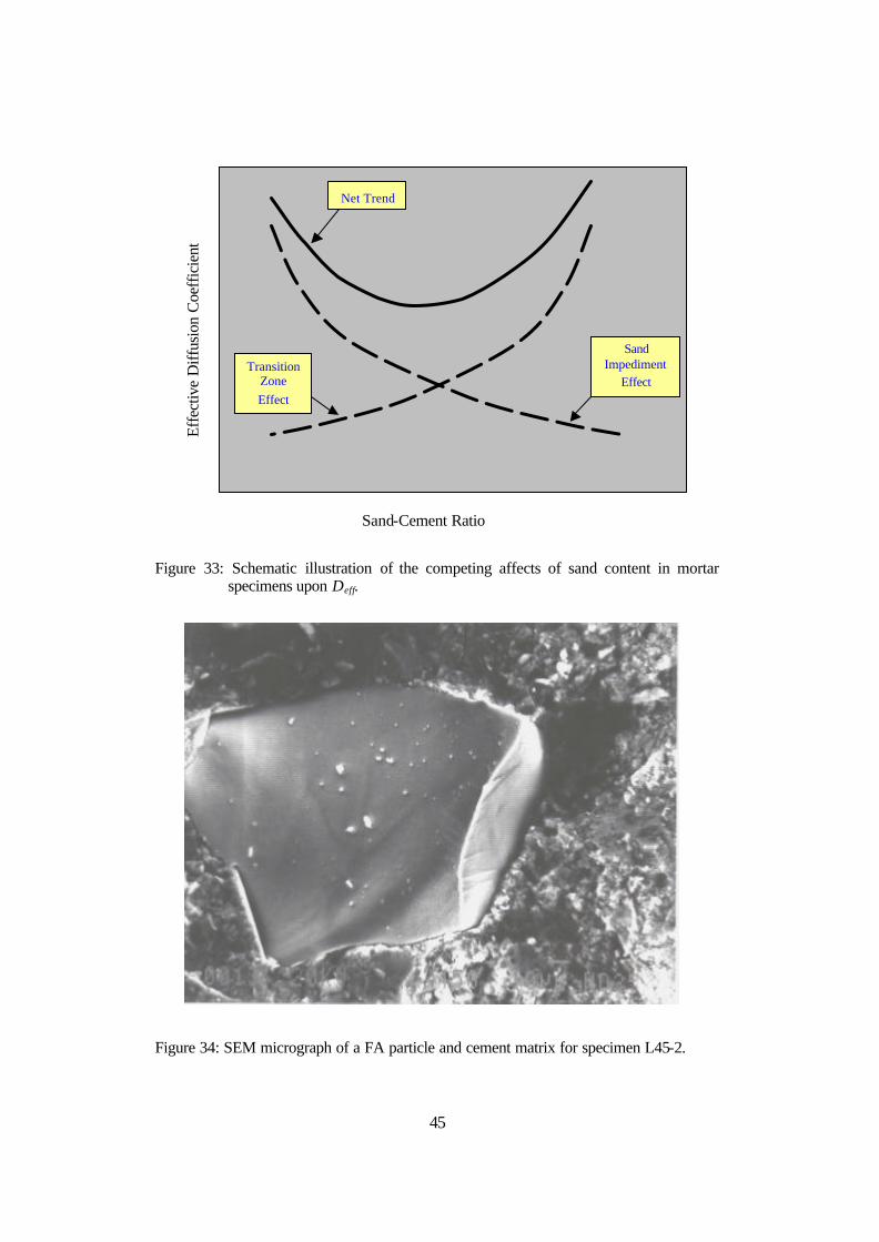
experiments suggest an effect of two competing processes where transition zone interconnectivity

dominated at high sand-cement ratio and aggregate related Cl- ingress impediment at low. Figure

33 illustrates this schematically. Alternatively, the low FM mortar specimens exhibited

interfacial separations to a greater extent than did the high FM silica sand or coarse aggregate

particles. This is in spite of the fact that 80 percent of the low FM fine aggregate was silica sand,

as noted above. Figure 34 shows a SEM micrograph of a FA particle with separations at the paste

45

Figure 33: Schematic illustration of the competing affects of sand content in mortar specimens upon Deff.

Figure 34: SEM micrograph of a FA particle and cement matrix for specimen L45-2.

Effe

ctiv

e D

iffus

ion

Coe

ffic

ient

Sand-Cement Ratio

Sand Impediment

Effect Transition

Zone Effect

Net Trend

46

interface. The possibility cannot be discounted, however, that the separations as seen here

occurred in conjunction with the mortar slice being fractured. Nonetheless, the finding that such

separations were more common in the low FM mortar specimens suggests a relatively weak

interfacial bond, as could arise from excess porosity.

Another possibility is that no transition zone of high Cl- permeability existed in the present

specimens at the time of analysis. If it were the case, some indication should have been

forthcoming from the EDX results in Figure 32, since the analysis spot dimensions approximated

thickness of any transition zone. Maso (24) reported that no transition zone was present in well

cured systems he investigated.

This observation that Deff for both FA types was minimal at a sand-cement ratio of about

unity (one-half in the case of the low FM mortar) and was elevated for a value of two, the effect

being greater for high compared to low FM mortar (see Tables 15 and 13, respectively), raises a

concern since common concrete mix designs often specify a ratio of about two. If this same

effect carries forth to concrete, then the high FM mortar specimen data (Table 15) indicate that a

two-fold reduction in Deff would be realized if the sand-cement ratio could be reduced to near one.

The determination that chlorides were present in the Ca-rich low FM fine aggregate but not

in the limestone CA could be size related. If this is the case, then it is important that the size

transition below which Cl- uptake occurred for limestone aggregates be determined and that this

serve as a lower limit for these CA in the case of concretes that are to be exposed to chlorides in

service. No such determination was made as a part of this study, however.

Significance of Surface Chloride Concentration

Virtually all of the Cl- analysis data and trends related thereto that were developed in the

present experiments point to both cs, and Deff, being important parameters with regard to Cl-

intrusion rate. In this regard, Equation 9 indicates a square root dependence of [Cl-] upon Deff,

whereas the dependence upon cs is according to a power of unity. Despite this, relatively little

attention has been focused in past research upon means whereby cs might be affected and

controlled. An exception is the work of Bamforth and Price (10) and Bamforth (9), who

identified 1) location, 2) physical aspects of exposure (for example, orientation, degree of shelter,

and micro-climate), 3) mix design variables, 4) curing variables, and 5) type of formwork, as

47

influential. Bamforth and Price summarized their own results for structures and specimens

undergoing coastal exposure in combination with data from the literature and concluded that,

first, cs apparently reached a steady-state value within the initial six months and, second, cs was

variable because of seasonal weather and surface washing. Most of the cs data for OPC concretes

were in the range 0.1-0.8 w/o concrete. Measured values for cs in the present concrete specimens

were 3-10 kg/m3 of concrete or 0.13-0.45 on a w/o basis, in general agreement with the

previously reported range. Bamforth (9) pointed out that cs increased with increasing cement

content, presence of pozollans, and increased curing time. This potentially poses a problem for

situations where mix design is durability driven, since Deff exhibits an opposite dependence upon

each of these three factors. If this is the case, then optimization of Cl- ingress resistance may

involve a tradeoff with these mix design variables. The latter two factors (pozzolans and curing

time) were not included in the present study. This importance of cs toward understanding the mix

design dependence of Cl- intrusion may be responsible for or have contributed to the relatively

poor correlation that has been reported between rapid permeability (charge gradient driven) and

natural diffusion (concentration gradient driven) results (20).

Figure 35 shows the present cs data on a w/o cement basis and indicates that, with three

exceptions, values are in the range 1.0-2.7 w/o cement. Also, while the concrete specimen data

show decreasing cs with increasing w/c, no definitive dependence of cs upon w/c is apparent for

mortars of either FA type. This cs-w/c trend for the concrete specimens is disappointing, although

it is consistent with the findings of Bamforth (9), because it indicates a negative consequence of

low w/c mix designs for Cl- exposure service, as noted above. The data suggest that research

regarding concrete surface treatments for the purpose of reducing cs could be advantageous. The

exceptions to the general trend whereby cs was in the range 1.0-2.7 w/o cement are the concrete

specimen SLF9, which had the lowest cement content, and specimens L45-2 and L55-2, which

had the highest sand-cement ratio (two). Thus, this sand-cement ratio not only elevated Deff,

compared to lesser ratios, as noted above, but it also resulted in relatively high values for cs. In

contrast to the above, Figure 36 plots cs versus Deff revealing a general trend suggesting that

material and mix design factors tend to have a common effect upon both parameters, albeit with

relatively large scatter. This general trend whereby high cs tended to result in high Deff may,

however, be an artifact of whatever factor(s) caused the outliers (high sand-cement ratio in the

case of mortars and low cement content for concrete); and so other aspects of mix design that

were not investigated might alter this.

48

Figure 35: Representation of surface Cl- concentration on a cement weight basis.

Figure 36: Plot of surface chloride concentration versus effective diffusion coefficient for mortar and concrete specimens.

0

1

2

3

4

5

0 1 2 3 4

Surf

ace

Chl

orid

e C

once

ntra

tion,

w/o

of

ConcreteLow FM Silica Sand FA High FM Silica Sand FA

0.38 0.45 0.55 Water-Cement Ratio

0.0

1.0

2.0

3.0

4.0

5.0

6.0

1.00E-13 1.00E-12 1.00E-11 1.00E-10

Effective Diffusion Coefficient, m2/s

Surf

ace

Chl

orid

e C

onc.

, w/o

cem

ent Concrete

Low FM Silica Sand FA High FM Silica Sand FA

49

ACKNOWLEDGEMENT

The authors express gratitude to Mr. George Jones for assistance with the experiments.

CONCLUSIONS

Mortar specimens with silica sand of either of two fineness moduli and concrete specimens

were cyclically wet-dry ponded with a ten w/o NaCl solution for approximately one year. Mix

design variables included 1) water-cement ratio (0.38, 0.45, and 0.52 (concrete specimens) or

0.55 (mortar specimens), 2) sand-cement ratio in the case of mortar specimens and fine

aggregate -coarse aggregate-cement ratio for concrete ones, 3) coarse aggregate type (porous

Florida limestone (SLF), dense Alabama limestone (VLA), and Ohio quartz (QO)), 4) coarse

aggregate grading (as-received, which was not within specification, and rescreened and regraded

(ideal), which was). The following conclusions were reached.

1. The effective chloride diffusion coefficient, Deff, and the surface chloride concentration, cs,

are both important parameters that affect the rate of chloride ingress and occurrence of

reinforcing steel corrosion and concrete cracking and spalling. Both parameters varied with

mix design.

2. Surface chloride concentration and Deff generally increased for the three specimen types in the

following order: concrete, high fineness modulus silica sand mortar, and low fineness

modulus silica sand mortar.

3. The Deff of mortar specimens was relatively low for the two intermediate sand-cement ratios

(0.5 and 1.0) and high for the two extremes (0 and 2.0). If this same trend applies to

concretes as well, then the mortar portion within concretes may be of relatively high chloride

permeability, since concretes are often designed with a sand-cement ratio of about two. This

trend, where Deff was relatively high at a sand-cement ratio of zero and two and low at 0.5 and

one, suggests two competing processes where, first, interconnectivity of a relatively porous

paste transition zone adjacent to aggregate particles, as has been reported from previous

research, was increasingly important with increasing sand-cement ratio and dominated at the

highest value (two) and, second, aggregate related chloride ingress impediment was

controlling in the lower sand-cement ratio range.

50

4. The Deff for specimens with water-cement ratio 0.38 was either about the same (mortar

specimens) or higher (concrete specimens) than for a ratio of 0.45. This is thought to have

resulted because a superplasticizer was not included in the mix design such that these

materials were stiff and difficult to place. Specimens with water-cement ratio 0.52 (concrete)

and 0.55 (mortar) invariably exhibited a higher Deff than for a ratio of 0.45. On this basis,

data for the 0.38 water-cement ratio specimens is considered suspect.

5. For concrete specimens with water-cement ratio 0.45, Deff increased in proportion to the

coarse aggregate -to-fine aggregate ratio, which was also in proportion to the volume fraction

of coarse aggregate.

6. The surface chloride concentration for the present specimens was generally in the range 1.0-

2.7 w/o cement (3-10 kg/m3 of concrete or 0.13-0.45 on a w/o basis) in general agreement

with the previously reported range.

7. The Iowa Pore Index for the SLF coa rse aggregate was 208/44, whereas the Indices for the

VLA and QO were 0/2 and 12/2, respectively. According to accepted interpretation of data

from this test, the SLF aggregate had well interconnected macro- and capillary pores and

should exhibit poor durability. The opposite is true for the VLA and QO aggregates.

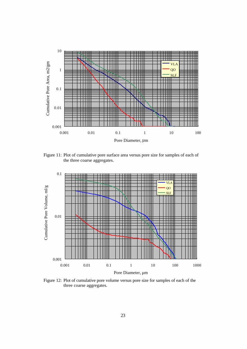
8. Results from intrusion mercury porosimetry tests indicated that the SLF aggregate had the

greatest cumulative concentration of pores and largest pore surface area. The VLA aggregate

had the greatest cumulative pore volume and surface area for relatively large pores, but these

parameters moderated in the capillary size range. Cumulative pore volume was lowest for the

QO aggregate; however, its cumulative pore surface area was approximately the same as for

the VLA. A disproportionate fraction of the QO material pore surface area was in the

smallest pore size range (less than 0.01 µm diameter).

9. The Deff for the concrete specimen fabricated using the SLF coarse aggregate was 16 and 26

percent higher than for the VLA and QO aggregates, respectively. This difference is

considered modest in view of the highly porous nature of the SLF material and the fact that

the QO is one of the densest aggregates in the United States. Apparently, coarse aggregate

pore structure is not a significant factor where concrete durability and service life are

controlled by chloride induced reinforcement corrosion. This finding suggests that the Iowa

51

Pore Index and mercury porosimetry results are not useful for qualifying or characterizing

coarse aggregates for such service.

10. The relatively high cs and Deff values for the low fineness modulus mortar specimens

compared to those for the high could have resulted from Cl- absorption by some of the Ca-

rich fine aggregate particles that were present. Alternatively, the smaller fine aggregate

particles may have provided less of an impediment to Cl- diffusion than the larger ones.

11. Grading of the as-received high fineness modulus fine aggregate and the as-received SLF

coarse aggregate did not conform to specification in that the particle size range in both cases

was too narrow with an absence of larger size particles. Concrete specimens fabricated using

these aggregates resulted in a higher Deff than ones for which the coarse aggregate was

rescreened and then regraded to within specification. For a water-cement ratio of 0.45, this

difference was by 16 percent.

12. The finding that aggregate grading did not conform to specification is thought to have

resulted from the materials handling procedure which involves the following steps:

a. Upon mining and crushing, the stone is separated into nine stockpiles according to size. b. The stone from these piles is then batched (blended) according to the specific job

specification.

c. The resultant CA is then loaded into a rail car and transported to a concrete plant.

d. Upon arrival at the concrete plant, the aggregate is bottom dumped into a silo. This results in an inverted cone with finer particles at the center and coarser at the outside.

e. The aggregate is transported upon a conveyer belt to the mixer. Both FDOT and plant

inspectors check the gradation every two-three months by taking three samplings from the belt at three different times, mixing these, and sieving.

The potential short-coming of this method is that the aggregate is segregated on the belt but

may be re-proportioned to within specification when the three segregated samples are mixed.

Consequently, the quality control procedure may be flawed.

13. Scanning electron microscopy and energy dispersive x-ray analysis of cores acquired from

the chloride exposed specimens indicated that concentration of this species (chlorides) in the

52

SLF coarse aggregate and high fineness modulus silica sand fine aggregate was below the

detection limit of the instrumentation. Chlorides were detected in the low fineness modulus

sand particles that were Ca-rich. This confirms the previous projection that chlorides migrate

through the cement paste only with the aggregates serving as an impediment to this transport

and is consistent with the finding that, first, Deff for specimens of each of the three coarse

aggregate types was generally the same and, second, some Deff reduction was affected by

specification compared to non-specification graded coarse aggregate.

RECOMMENDATIONS

Based upon the results of this research, the following are recommended:

1. A statistically significant survey of fine and coarse aggregate grading that is being realized in

Florida bridge construction should be performed. This could be accomplished by sampling

fresh concrete at construction sites about the State, washing the material, and screening. By

comparison of these gradings with results of this research, it should be possible to estimate

the Deff improvement that could be realized if the aggregate grading was within specification.

2. It was determined that chlorides were present in the Ca-rich fine aggregate particles, whereas

this species was absent in the coarse aggregate. Apparently, the propensity for chlorides to be

present in Florida limestone aggregates is size dependent. The size or size range at with this

transition occurs should be determined.

3. Studies of mix design improvements that can be affected based upon fine and coarse

aggregate gradings should be continued.

BIBLIOGRAPHY

1. Hausmann, D.A., Materials Protection, Vol. 6(10), 1967, p. 23. 2. Gouda, V.K., British Corrosion Journal, Vol. 5, 1970, p. 198. 3. Hausmann, D.A., Materials Performance, Vol. 37(10), 1998, p. 64. 4. Breit, W., Mater. Corrosion, Vol. 49, 1998, p. 539.

53

5. Charvin, S., Hartt, W.H., and Lee, S. K., “Influence of Permeability Reducing and Corrosion Inhibiting Admixtures in concrete upon Initiation of Salt Induced Embedded Steel Corrosion,” paper no. 00802 presented at CORROSION/00, March 26-31, 2000, Orlando.

6. Li, L. and Sagüés, A.A., Corrosion, Vol. 57, 2001, p. 19. 7. Glass, G.K. and Buenfeld, N.R., “Chloride Threshold Levels for Corrosion Induced

Deterioration of Steel in Concrete,” paper no. 3 presented at RILEM International Workshop on Chloride penetration into Concrete, Oct. 15-18, 1995, Saint Rémy-les-Chevreuse.

8. Tutti, K., Corrosion of Steel in Concrete, Report No. Fo 4, Swedish Cement and Concrete

Research Institute, Stockholm, 1982. 9. Bamforth, P.B., “Definition of Exposure Classes and Concrete Mix Requirements for

Chloride Contaminated Environments,” Corrosion of Reinforcement in Concrete , Eds: Page, C.L., Treadaway, K.W.J., and Bamforth, P.B., Soc. Chem. Ind., London, 1996, p. 176.

10. Bamforth, P.B. and Price, W.F., “Factors Influencing Chloride Ingress into Marine

Structures,” Concrete 2000 , Eds: Dhir, R.K. and Jones, M.R., E&FN Spon, London, 1993, p. 1105.

11. Thompson, N.G. and Lankard, D.L., “Improved Concretes for Corrosion Resistance,” Report

No. FHWA-RD-96-207, Federal Highway Administration, 1997. 12. “Specification for Concrete Aggregates,” ASTMC33-01, Annual Book of Standards,

American Society for Testing and Materials, 100 Barr Harbor Drive, West Conshohocken, PA 19428.

13. “Florida Method of Test for Determining Low-Levels of Chloride in Concrete and Raw

Materials,” Designation FM 5-516, Florida Department of Transportation, Tallahassee, FL, Sept., 1994.

14. Mr. Jerry Haught, Rinker Materials Corporation, West Palm Beach, FL, personal

communication. 15. Eades, J.L., McClellan, G.H., and Fountain, K.B., “Evaluation of Soundness Tests on Florida

Aggregates”, Final Report, FDOT Contract B-8354 (WPI 0510682), March, 1997. 16. Bamforth, P.B. and Pocock, D.C., “Minimizing the Risk of Chloride Induced Corrosion by

Selection of Concreting Materials,” Corrosion of Reinforcement in Concrete, Ed: Page, C.L., Treadaway, K.W.J., and Bamforth, P.B., Soc. Chemical Ind., London, 1990.

17. Diederichs, V., Hinrichsmeyer, K., and Schneider, U., “Analysis of Thermal, Hydrothermal,

and Mechanical Stresses of Concrete by Mercury-Porosimetry and Nitrogen-Sorption,” Proceedings, RILEM/CNR International Symposium of Principles and Applications of Pore Structural Characterization, Milan, April, 1983.

18. Winslow, D.N., The Pore Structure and Surface Area of Hydrated Portland Cement Paste,” in

Characterization and Performance Prediction of Cement and Concrete , Ed. J.F. Young, Engr. Foundation, New York, 1984, p. 105.

54

19. Winslow, D.N. and Liu, D., Cement and Concrete Research, Vol. 20, 1990, p. 227. 20. Winslow, D.N. Cohen, M.D., Bentz, D.P., Snyder, K.A., and Garboczi, E.J.., Cement and

Concrete Research, Vol. 24, 1994, p. 25. 21. Halamickova, P., Detwiler, R.J., Bentz, D.P., and Garboczi, E.J., Cement and Concrete

Research, Vol. 25, 1995, p. 790. 22. Young, J.F., “A Review of the Pore Structure of Cement Paste and Concrete and Its Influence

on Permeability,” in Permeability of Concrete , Eds. D. Whiting and A. Walitt, ACI SP-108, American Concrete Institute, 1988, p. 1.

23. Andrade, C., Sanjuán, M.A., Recuero, A., and Río, O., Cement and Concrete Research, Vol.

24, 1994, p. 1214. 24. Maso, J. C., “The Bond between Aggregates and Hydrated Cement Pastes,” Proceedings,

Seventh International Conference on the Chemistry of Cement, Vol. 1, Paris, 1980, p. VII-1.