A unified Petrov–Galerkin spectral method for fractional PDEs€¦ · Petrov–Galerkin (DPG) and...

$Page 1: A unified Petrov–Galerkin spectral method for fractional PDEs€¦ · Petrov–Galerkin (DPG) and a discontinuous Galerkin (DG) method for the hyperbolic time- and space-fractional$
Available online at www.sciencedirect.com

ScienceDirect

Comput. Methods Appl. Mech. Engrg. 283 (2015) 1545–1569www.elsevier.com/locate/cma

A unified Petrov–Galerkin spectral method for fractional PDEs

Mohsen Zayernouri, Mark Ainsworth, George Em Karniadakis∗

Division of Applied Mathematics, Brown University, 182 George Street, Providence, RI 02912, USA

Received 3 January 2014; received in revised form 29 October 2014; accepted 31 October 2014Available online 7 November 2014

Abstract

Existing numerical methods for fractional PDEs suffer from low accuracy and inefficiency in dealing with three-dimensionalproblems or with long-time integrations. We develop a unified and spectrally accurate Petrov–Galerkin (PG) spectral methodfor a weak formulation of the general linear Fractional Partial Differential Equations (FPDEs) of the form 0 D2τ

t u +d

j=1 c j

[a j D2µ jx j u ] + γ u = f , where 2τ , µ j ∈ (0, 1), in a (1 + d)-dimensional space–time domain subject to Dirichlet initial and

boundary conditions. We perform the stability analysis (in 1-D) and the corresponding convergence study of the scheme (in multi-D). The unified PG spectral method applies to the entire family of linear hyperbolic-, parabolic- and elli ptic-like equations.We develop the PG method based on a new spectral theory for fractional Sturm–Liouville problems (FSLPs), recently introducedin Zayernouri and Karniadakis (2013). Specifically, we employ the eigenfunctions of the FSLP of first kind (FSLP-I), called Ja-cobi poly-fractonomials, as temporal/spatial bases. Next, we construct a different space for test functions from poly-fractonomialeigenfunctions of the FSLP of second kind (FSLP-II). Besides the high-order spatial accuracy of the PG method, we demon-strate its efficiency and spectral accuracy in time-integration schemes for solving time-dependent FPDEs as well, rather thanemploying algebraically accurate traditional methods, especially when 2τ = 1. Finally, we formulate a general fast linear solverbased on the eigenpairs of the corresponding temporal and spatial mass matrices with respect to the stiffness matrices, whichreduces the computational cost drastically. We demonstrate that this framework can reduce to hyperbolic FPDEs such as time-and space-fractional advection (TSFA), parabolic FPDEs such as time- and space-fractional diffusion (TSFD) model, and ellipticFPDEs such as fractional Helmholtz/Poisson equations with the same ease and cost. Several numerical tests confirm the efficiencyand spectral convergence of the unified PG spectral method for the aforementioned families of FPDEs. Moreover, we demon-strate the computational efficiency of the new approach in higher-dimensions e.g., (1 + 3), (1 + 5) and (1 + 9)-dimensionalproblems.c⃝ 2014 Elsevier B.V. All rights reserved.

Keywords: Jacobi poly-fractonomial; Fractional basis/test functions; Unified fast FPDE solver; Spectral convergence

1. Introduction

The calculus of fractional differentiation and fractional integration generalizes the notion of the standard integer-order calculus to any real-valued order [1,2]. Over the last decades, it has been shown that fractional differential

∗ Corresponding author. Fax: +1 401 863 2722.E-mail address: george [email protected] (G.E. Karniadakis).

http://dx.doi.org/10.1016/j.cma.2014.10.0510045-7825/ c⃝ 2014 Elsevier B.V. All rights reserved.

http://crossmark.crossref.org/dialog/?doi=10.1016/j.cma.2014.10.051&domain=pdf

http://www.elsevier.com/locate/cma

http://dx.doi.org/10.1016/j.cma.2014.10.051

http://www.elsevier.com/locate/cma

mailto:[email protected]

http://dx.doi.org/10.1016/j.cma.2014.10.051

1546 M. Zayernouri et al. / Comput. Methods Appl. Mech. Engrg. 283 (2015) 1545–1569

operators appear as attractive and potentially powerful modeling tools in many areas such as viscoelastic materials[3,4], porous or fractured media [5], fluid mechanics [6–8], bioengineering [9], and anomalous diffusion (non-Markovian) processes [10,11]. In these applications, fractional partial differential equations (FPDEs) appear of differ-ent type such as time- and/or space-fractional diffusion equation of parabolic nature [12], time- and/or space fractionaladvection, advection–diffusion and Burger’s equations of hyperbolic character [13,14], also elliptic FPDEs as the sta-tionary space-fractional diffusion problems [15].

Existing numerical schemes for FPDEs suffer mainly from low accuracy and computational inefficiency in dealingwith three-dimensional problems or with long-time integrations. Recently, a variety of numerical methods, originallydeveloped for integer-order PDEs (see e.g., [16–19]), have been extended to FPDEs. Such an extension is neithertrivial nor straightforward. For instance, there is a lot of work done in developing Finite-Difference Methods (FDM)for FPDEs. Lubich [20,21] introduced the idea of discretized fractional calculus and later Sanz-Serna [22] presenteda first-order FDM algorithm for partial integro-differential equations. Since then, many works have aimed at improv-ing the convergence rates of FDM schemes e.g., in time to (∆t)2−α or (∆t)3+α, α ∈ (0, 1) (see e.g.[23–26]). Theimplementation of such FDM approaches is relatively easy. However, the bottleneck in the FDM approach is that theconvergence is algebraic and the accuracy is limited. Moreover, we observe that the heavy cost and memory storagein computing the long-range history in two- and three-dimensional problems makes FDM schemes computationallyinefficient. In fact, FDM is essentially a local approach which has been employed to approximate non-local fractionalderivatives. This fact would suggest that global schemes, such as spectral methods (SM), are more consistent/adaptedto the nature of FPDEs.

Sugimoto [14] employed Fourier SM in fractional Burgers’ equation, and later Blank [27] adopted a spline-basedcollocation method for a class of FODEs. This approach was later employed by Rawashdeh [28] for solving fractionalintegro-differential equations. Li and Xu [29,30] developed a space–time spectral method for a time-fractionaldiffusion equation with spectral convergence, which was based on the early work of Fix and Roop [31]. Later on,Khader [32] proposed a Chebyshev collocation method for a space-fractional diffusion equation; also Piret and Hanertdeveloped a radial basis function method for fractional diffusion equations [33]. Moreover, a Chebyshev spectralmethod [34], a Legendre spectral method [35], and an adaptive pseudospectral method [36] were proposed for solvingfractional boundary value problems. In addition, generalized Laguerre spectral algorithms and Legendre spectralGalerkin method were developed by Baleanu et al. [37] and by Bhrawy and Alghamdia [38] for fractional initialvalue problems, respectively. The main challenge in these spectral methods is that the corresponding stiffness andmass matrices are non-symmetric, dense and they gradually become ill-conditioned when the fractional order tends tosmall values. Hence, carrying out long-time and/or adaptive integration using such SM schemes becomes intractable.To this end, Xu and Hesthaven [39] developed a stable multi-domain spectral penalty method for fractional partialdifferential equations. In all the aforementioned studies, the standard integer-ordered (polynomial) basis functionshave been utilized.

Recently, Zayernouri and Karniadakis [40,41] developed spectrally accurate Petrov–Galerkin spectral and spectralelement methods for non-delay and delay fractional differential equations, where they employed a new family offractional bases, called Jacobi poly-fractonomials. They introduced these poly-fractonomials as the eigenfunctions offractional Sturm–Liouville problems in [42], explicitly given as

(1)Pα,β,µn (ξ) = (1 + ξ)−β+µ−1 Pα−µ+1,−β+µ−1

n−1 (ξ), ξ ∈ [−1, 1], (1)

with µ ∈ (0, 1),−1 ≤ α < 2 − µ, and −1 ≤ β < µ − 1, which are representing the eigenfunctions of the singularFSLP of first kind (SFSLP-I), and

(2)Pα,β,µn (ξ) = (1 − ξ)−α+µ−1 P−α+µ−1, β−µ+1

n−1 (ξ), ξ ∈ [−1, 1], (2)

where −1 < α < µ − 1 and −1 < β < 2 − µ, and µ ∈ (0, 1), denoting the eigenfunctions of the singularFSLP of second kind (SFSLP-II). Moreover, Zayernouri and Karniadakis developed a space–time discontinuousPetrov–Galerkin (DPG) and a discontinuous Galerkin (DG) method for the hyperbolic time- and space-fractionaladvection equation in [43]. This approach was shown to be also applicable to problems of integer order timederivatives. In addition, they employed the aforementioned Jacobi poly-fractonomial bases to introduce a newclass of fractional Lagrange interpolants for developing an efficient and spectrally accurate Fractional SpectralCollocation Method (FSCM) in [44] for a variety of FODEs and FPDEs including multi-term FPDEs and the nonlinear

M. Zayernouri et al. / Comput. Methods Appl. Mech. Engrg. 283 (2015) 1545–1569 1547

space-fractional Burgers’ equation. Recently, the FSCM scheme has been further generalized to FPDEs of variableorder in [45], in where the associate fractional order(s) can vary in the computational domain Ω . However, like allprevious spectral methods, applying these schemes to higher-dimensional problems remains a great challenge.

In this paper, we develop a unified and spectrally accurate Petrov–Galerkin (PG) spectral method for the generalFPDEs of the following weak form

(0 Dτt u, t Dτ

T v)Ω +

dj=1

c j (a j Dµ jx j u, x j Dµ j

b jv)Ω + γ (u, v)Ω = ( f, v)Ω ,

where 2τ, µ j ∈ (0, 1), in a (1 + d)-dimensional space–time domain subject to Dirichlet initial and boundary condi-

tions. Such a weak form is equivalent to the strong form 0 D2τt u +

dj=1 cx j a j D2µ j

x j u + γ u = f , when u possessesenough smoothness. This method applies equally-well to the entire family of linear fractional hyperbolic, parabolicand elli ptic equations with the same ease. The main feature of this PG spectral methods is the global discretizationof the temporal term, in addition to the spatial derivatives, rather than utilizing traditional low-order time-integrationmethods. We essentially develop our PG method based on a new spectral theory for fractional Sturm–Liouville prob-lems (FSLPs) [42]. Specifically, we employ the eigenfunctions of the FSLP of first kind (FSLP-I), called Jacobi poly-fractonomials, as temporal/spatial bases. Next, we construct a different space for test functions from poly-fractonomialeigenfunctions of the FSLP of second kind (FSLP-II). We show that this choice of basis and test functions leads toa stable bilinear form; moreover, we perform the corresponding error analysis. In the present method, all the afore-mentioned matrices are constructed exactly and efficiently. Moreover, we formulate a new general fast linear solverbased on the eigenpairs of the corresponding temporal and spatial mass matrices with respect to the stiffness matri-ces, which significantly reduces the computational cost in higher-dimensional problems e.g., (1 + 3), (1 + 5) and(1 + 9)-dimensional FPDEs.

The organization of the paper is as follows: in Section 2, we introduce the notation and some preliminaries fromfractional calculus. In Section 3, we present the mathematical formulation of the Petrov–Galerkin spectral methodin a (1 + d)-dimensional hypercube where we define the basis and test function spaces separately. We additionallyobtain the general Lyapunov equation, for which we formulate a closed-form solution in terms of the generalizedeigensolutions. In Section 4, we reduce this general framework to the special well-known (i) hyperbolic, (ii) parabolicFPDEs, and (iii) elliptic FPDEs. We furthermore employ our PG method and the fast solver to even higher dimensional(10-D) problems to demonstrate the robustness and applicability of the scheme. In addition, we introduce our schemeas a spectrally accurate time-integrator method when the FPDE of interest is integer-order in time. We end the paperwith a summary and discussion in Section 5. In the Appendix, we present the properties of the stiffness and massmatrices and provide efficient quadrature rules to compute them exactly.

2. Preliminaries on fractional calculus

We first provide some definitions from fractional calculus. Following [2], for a univariate function g(x) ∈ Cn[a, b],

we denote by a Dνx g(x) the left-sided Riemann–Liouville fractional derivative of order ν, when n−1 ≤ ν < n, defined

as

a Dνx g(x) =

1Γ (n − ν)

dn

dxn

x

a

g(s)

(x − s)ν+1−nds, x ∈ [a, b], (3)

where Γ represents the Euler gamma function, and as ν → n, the global operator a Dνx → dn/dxn , recovering

the local nth order derivative with respect to x . We also denote by x Dνb g(x) the corresponding right-sided

Riemann–Liouville fractional derivative of order ν, defined as

b Dνx g(x) =

1Γ (n − ν)

(−1)ndn

dxn

b

x

g(s)

(s − x)ν+1−nds, x ∈ [a, b]. (4)

Similarly, as ν → n, the right-sided fractional derivative tends to the standard nth local one. The correspondingleft- and right-sided fractional derivative of Caputo type can be also defined as (3) and (4), but with the order ofintegration and differentiation exchanged. However, these two sets of Riemann–Liouville and Caputo definitions are


closely linked. By virtue of (3) and (4), we can define the corresponding partial fractional-derivative of a bivariatefunction.

Finally, we recall a useful property of the Riemann–Liouville fractional derivatives. Assume that 0 < p < 1 and0 < q < 1 and g(xL) = 0 x > xL , then

xL D p+qx g(x) =

xL D p

x

xL Dqx

g(x) =

xL Dqx

xL D px

g(x). (5)

3. Mathematical formulation of Petrov–Galerkin spectral method

Let u : Rd+1→ R, for some positive integer d. For u ∈ U (see e.g., (10)), we consider the following general weak

form in Ω = [0, T ] × [a1, b1] × [a2, b2] × · · · × [ad , bd ] as

(0 Dτt u, t Dτ

T v)Ω +

dj=1


b jv)Ω + γ (u, v)Ω = ( f, v)Ω , ∀v ∈ V, (6)

where γ, c j are constant, 2τ, µ j ∈ (0, 1), j = 1, 2, . . . , d , subject to the following homogeneous Dirichlet initial andboundary conditions

u|t=0 = 0, τ ∈ (0, 1/2), (7)

u|x j =a j = 0, µ j ∈ (0, 1/2), j = 1, 2, . . . , d

u|x j =a j = u|x j =b j = 0, µ j ∈ (1/2, 1), j = 1, 2, . . . , d.

We note that the variational form (6) is equivalent to the following linear FPDE of order 2τ in time and 2µ j in the j thspatial dimension, j = 1, 2, . . . , d,

0 D2τt u(t, x1, x2, . . . , xd)+

dj=1

c j [ a j D2µ jx j u(t, x1, x2, . . . , xd) ] + γ u(t, x1, x2, . . . , xd)

= f (t, x1, x2, . . . , xd), (8)

when solution u is smooth enough.We define the solution space U as

U :=

u : Ω → R | u ∈ C(Ω), ∥u∥U < ∞, and u|t=0 = u|x j =a j = 0

, (9)

if µ j ∈ (0, 1/2) and

U :=

u : Ω → R | u ∈ C(Ω), ∥u∥U < ∞, s.t. u|t=0 = u|x j =a j = u|x j =b j = 0

(10)

when µ j ∈ (1/2, 1), in which

∥u∥U =

∥0 Dτ

t u∥2+

dj=1

∥a j Dµ jx j u∥

2+ ∥u∥

21/2

. (11)

Correspondingly, we define the test space V as

V :=

v : Ω → R | ∥v∥V < ∞, s.t. v|t=T = v|x j =b j = 0

, (12)

when µ j ∈ (0, 1), in which

∥v∥V =

∥t Dτ

T v∥2+

dj=1

∥x j Dµ jb jv∥2

+ ∥v∥21/2

, (13)


where by [31,46], we can show that U and V are Hilbert spaces, moreover, the associated norms ∥ · ∥U and ∥ · ∥V areequivalent. Now, let a : U × V → R be a bilinear form, defined as

a(u, v) = (0 Dτt u, t Dτ

T v)Ω +

dj=1


b jv)Ω + γ (u, v)Ω . (14)

Moreover, let L ∈ V ∗, the dual space of V , be a continuous linear functional defined as

L(v) = ( f, v), ∀v ∈ V . (15)

Now, the problem is to find u ∈ U such that

a(u, v) = L(v), ∀v ∈ V . (16)

Next, we define UN ⊂ U and VN ⊂ V to be finite dimensional subspaces of U and V with dim(UN ) = dim(VN ) = N .Now, our PG spectral method reads as: find uN ∈ UN such that

a(uN , vN ) = L(vN ), ∀vN ∈ VN . (17)

By representing uN as a linear combination of points/elements in UN i.e., the corresponding (1 + d)-dimensionalspace–time basis functions, the finite-dimensional problem (17) leads to a linear system known as Lyapunov matrixequation. For instance, if d = 1, i.e., 1-D in time and 1-D in space, we obtain the corresponding Lyapunov equationin the space–time domain [0, T ] × [a1, b1] as

Sτ U MTµ1

+ Mτ U STµ1

= F, (18)

in which U is the matrix of unknown coefficients, Sτ and Mτ denote, respectively, the temporal stiffness and massmatrices; similarly, Sµ1 and Mµ1 , represent the spatial stiffness and mass matrices, and F is the corresponding loadmatrix.

In general, numerical solutions to such a linear system, originating from a fractional differential operator, becomeexcessively expensive since the corresponding mass and stiffness matrices usually turn out to be full and non-symmetric. Moreover, we note that the size of the above linear system grows as the product of the degrees offreedom in each dimension. To address this problem in this paper, we present a new class of basis and test functionsyielding stiffness matrices, which are either diagonal or tridiagonal. Similarly, by introducing proper quadraturerules, we compute exactly the corresponding mass matrices, which are symmetric. Such useful properties allow usto subsequently develop a general fast linear solver for (18) with a substantially reduced computational cost. To thisend, we first introduce the corresponding finite-dimensional spaces of basis UN and test functions VN in our PGframework.

3.1. Space of basis functions (UN )

We develop a PG spectral method for (8), subject to homogeneous Dirichlet initial and boundary conditions. Weconstruct the basis function space as the space of some temporal and spatial functions to globally treat the time-dimension in addition to the spatial-dimensions. To this end, the new eigensolutions, introduced in [42], yield newsets of basis and test functions, properly suited for our Petrov–Galerkin framework. We represent the solution in theentire space–time computational domain Ω in terms of specially chosen basis functions, constructed as the tensorproduct of the eigenfunctions in the following manner. Let

(1)Pµn (ξ) = (1 + ξ)µ P−µ,µ

n−1 (ξ), n = 1, 2, . . . x ∈ [−1, 1], (19)

denote the eigenfunctions of the regular FSLP of first kind (RFSLP-I), corresponding to the case where α = β = −1.We construct our basis for the spatial discretization using the univariate poly-fractonomials defined by

φ µm ( ξ ) = σm

(1)P µ

m ( ξ ), m = 1, 2, . . . , µ ∈ (0, 1/2],

(1)P µm ( ξ )− ϵ µm

(1)P µm−1( ξ ), m = 2, 3, . . . µ ∈ (1/2, 1),

(20)


where σm = 2+(−1)m and theµ-dependent coefficient ϵµm j = (m−1−µ)/(m−1). The definition reflects the fact thatif µ ≤ 1/2 then only one boundary condition needs to be presented, whereas if µ > 1/2 then two endpoint conditionsare prescribed. Naturally, for the temporal basis functions only initial conditions are prescribed and as a consequencethe basis functions for the temporal discretization are constructed using the univariate poly-fractonomials

ψ τn (η) = σn

(1)P τn ( η ), τ ∈ (0, 1), (21)

for n ≥ ⌈2τ⌉. With these notations established, we define the space–time trial space to be

UN = spanψ τ

n η(t)

dj=1

φµx jm j ξ j

(x j ) : n = 1, . . . ,N , m j = ⌈σ j⌉, . . . ,M j

, (22)

where η(t) = 2t/T − 1 and ξ j (s) = 2 s−a jb j −a j

− 1. The construction of the univariate functions ensures that UN ⊂ U ,

since φ µm (−1) = 0, for all µ ∈ (0, 1), also φ µm (1) = 0, for all µ ∈ (1/2, 1). Then, we shall approximate the solutionto (8) in terms of a linear combination of elements in UN , whose bases satisfy exactly the homogeneous initial andboundary condition in Ω .

3.2. Space of test functions (VN )

Let the poly-fractonomials

(2)P µk (ξ) = (1 − ξ)µ P µ,−µ

k−1 (ξ), k = 1, 2, . . . , ξ ∈ [−1, 1], (23)

denote the eigenfunctions of the regular FSLP of second kind (RFSLP-II), corresponding to the case α = β = −1 in(2). Next, we construct our spatial test functions using the univariate poly-fractonomials defined by

Φ µk (ξ) = σk

(2)P µ

k ( ξ ), k = 1, 2, . . . µ ∈ (0, 1/2],(2)P µ

k (ξ)+ ϵµk(2)P µ

k−1(ξ), k = 2, 3, . . . µ ∈ (1/2, 1),(24)

where σk = 2 (−1)k + 1. Next, we define the temporal test functions using the univariate poly-fractonomials

Ψ τr (η) = σr

(2)P τr ( η ), τ ∈ (0, 1), (25)

for all r ≥ ⌈2τ⌉. With these notations established, we define the space–time test space to be

VN = span

Ψ τr η

(t)

dj=1

Φµ jk j

ξ j

(x j ) : r = 1, . . . ,N , k j = ⌈σ j⌉, . . . ,M j

. (26)

Having defined the space of trial and test functions, we can now define the corresponding temporal/spatial stiffnessand mass matrices.

Remark 3.1. We show later that the choice of σm in (20) and (21), also σk in (24) and (25), leads to the constructionof symmetric spatial/temporal mass and stiffness matrices. We will exploit this property to formulate a general fastlinear solver for the resulting linear system.

3.3. Stability and convergence analysis

The following theorems provide the stability analysis of the scheme when the pair of UN ⊂ U and VN ⊂ V aregiven as in (22) and (26), respectively. We first consider the discrete stability of the method for one-dimensional case.

Theorem 3.2. The Petrov–Galerkin spectral method for the problem

−1 D2µx u(x) = f (x), ∀x ∈ [−1, 1], (27)

u(−1) = 0, if 0 < µ < 1/2,

u(±1) = 0, if 1/2 < µ < 1


is stable, i.e., the discrete inf - sup condition

supvN ∈VN

a(uN , vN )

∥vN ∥V≥ β∥uN ∥U , ∀uN ∈ UN ⊂ U, (28)

holds with β = 1.

Proof. We note that in the absence of the time-derivative and since γ = 0, the corresponding norm defined onU (see Eq. (11)) just reduces to ∥u∥U = ∥−1 Dµ

x u∥. While ∥−1 Dµx u∥ has been traditionally treated as a semi-

norm in the literature (e.g., see [47,29]), one can easily show that it satisfies all the properties of a norm since theRiemann–Liouville fractional derivative of a constant is non-zero. Correspondingly, in this one-dimensional setting,∥v∥V = ∥x Dµ

1 v∥.

Case (I) 0 < µ < 1/2: we represent uN as

uN (x) =

Nn=1

un(1 + x)µP−µ,µn−1 (x), (29)

and choose vN to be the following linear combination of elements in VN as

vN (x) =

Nk=1

uk(1 − x)µPµ,−µk−1 (x), (30)

in which we employ the same coefficients uk as in (29). Hence, we obtain

a(uN , vN ) =

1

−1−1 Dµ

x uN x Dµ1 vN dt

=

Nn=1

un

Nk=1

uk

1

−1−1 Dµ

x [(1 + x)µP−µ,µn−1 (x)], x Dµ

1 [(1 − x)µPµ,−µk−1 (x)] dt

=

Nn=1

unΓ (n + µ)

Γ (n)

Nk=1

ukΓ (k + µ)

Γ (k)

1

−1Pn−1(x)Pk−1(x) dt

=

Nn=1

u2n

Γ (n + µ)

Γ (n)

2 2n + 12

= ∥x Dµ1 vN ∥

2L2([−1,1])

= ∥vN ∥2V , (31)

supvN ∈VN

a(uN , vN )

∥vN ∥V= ∥uN ∥U , ∀uN ∈ UN , (32)

which means that the stability is guaranteed for β = 1.

Case (II) 1/2 < µ < 1: we expand uN this time as

uN (x) =

Nn=1

un

(1 + x)µP−µ,µ

n−1 (x)− ϵµn (1 + x)µP−µ,µn−2 (x)

, (33)

and choose vN to be the following linear combination of elements in VN as

vN (x) =

Nk=1

uk

(1 − x)µPµ,−µk−1 (x)+ ϵ

µk (1 − x)µPµ,−µk−2 (x)

, (34)

where the coefficients uk are the same as the ones in (33). Hence, it is easy to again show that

a(uN , vN ) =

Nn=1

u2n

Γ (n + µ)

Γ (n)

2 2n + 12

(1 − ϵµn I1≤n≤N−1)

= ∥x Dµ1 vN ∥

2L2([−1,1])

= ∥vN ∥2V . (35)


Remark 3.3. We performed the discrete stability analysis for the 1-D case. The multi-D case is more involved andwe will address it in a separate paper in future.

Theorem 3.4 (Projection Error). In the weak form (17), let ∥0 Dr+τt u∥L2(Ω) < ∞ and ∥−1 Dr+µ j

x j u∥L2(Ω) < ∞ forall j = 1, 2, . . . , d, for some integer r ≥ 1. Moreover, let uN denote the projection of the exact solution u.Then,

∥u − uN ∥2U ≤ C N−2r

∥0 Dr+τ

t u∥2L2(Ω) +

dj=1

∥−1 Dr+µ jx j u∥

2L2(Ω)

.

Proof. We first consider the one-dimensional problem (27). We expand the exact solution u, when 2µ ∈ (0, 1), interms of the following infinite series of Jacobi poly-fractonomials

u(x) =

∞n=1

un(1 + x)µP−µ,µn−1 (x). (36)

Here, we would like to bound ∥u − uN ∥U in terms of higher-order derivative. We first note that

−1 Dr+µx u(x) =

dr

dxr [−1 Dµx u(x)] =

∞n=1

unΓ (n + µ)

Γ (n)dr

dxr [Pn−1(x)],

where

dr

dxr [Pn−1(x)] =

(n − 1 + r)!

2r(n − 1)!Pr,r

n−1−r (x), r ≤ n,

0, r > n.

Hence,

−1 Dr+µx u(x) =

∞n=r

unΓ (n + µ)

Γ (n)(n − 1 + r)!

2r(n − 1)!Pr,r

n−1−r (x).

Therefore,

∥(1 − x)r/2(1 + x)r/2−1 Dr+µx u(x)∥2

=

1

−1(1 − x)r (1 + x)r

∞n=r

unΓ (n + µ)

Γ (n)(n − 1 + r)!

2r(n − 1)!Pr,r

n−1−r (x)2

=

∞n=r

un

Γ (n + µ)

Γ (n)(n − 1 + r)!

2r(n − 1)!

2 1

−1(1 − x)r (1 + x)r Pr,r

n−1−r (x)Pr,rn−1−r (x)dx

=

∞n=r

un

Γ (n + µ)

Γ (n)(n − 1 + r)!

2r(n − 1)!

2 22r+1 ((n − 1)!)2

(n − 1 − r)!(n − 1 + r)!

=

∞n=r

un

Γ (n + µ)

Γ (n)

2 22n + 1

(n − 1 + r)!

(n − 1 − r)!.

We also note that (n−1+r)!(n−1−r)! is minimized when n = N + 1. Hence,

∥u − uN ∥2U =

∞n=N+1

un

Γ (n + µ)

Γ (n)

2

≤

∞n=N+1

un

Γ (n + µ)

Γ (n)

2 (n − 1 + r)!

(n − 1 − r)!

(N − r)!

(N + r)!

=(N − r)!

(N + r)!

∞n=N+1

un

Γ (n + µ)

Γ (n)

2 (n − 1 + r)!

(n − 1 − r)!,


=(N − r)!

(N + r)!∥(1 − x)r/2(1 + x)r/2−1 Dr+µ

x u(x)∥2

≤(N − r)!

(N + r)!∥−1 Dr+µ

x u(x)∥2

≤ c N−2r∥−1 Dr+µ

x u(x)∥2, (37)

where r ≥ 1 and 2µ ∈ (0, 1). Similar steps are done for the case 2µ ∈ (1, 2) to obtain (37) noting that in either case,µ remains between 0 and 1.

Next, we consider the following two-dimensional problem in Ω = [−1, 1] × [−1, 1]:

−1 D2µxx u(x, y)+ −1 D2µy

y u(x, y) = f (x, y), ∀(x, y) ∈ Ω , (38)

u(−1, y) = u(x,−1) = 0, if 0 < µx , µy < 1/2,

whose corresponding weak form is given by

(−1 Dµxx u, x Dµx

1 v)Ω + (−1 Dµyy u, y Dµy

1 v)Ω = ( f, v)Ω . (39)

We represent the exact solution u when 2µx , 2µy ∈ (0, 1), in terms of the following infinite series of tensor productJacobi poly-fractonomials as

u(x, y) =

∞n=1

∞m=1

unm(1 + x)µx P−µx ,µxn−1 (x) (1 + y)µy P

−µy ,µym−1 (y). (40)

Hence,

−1 Dr+µxx u =

∞n=1

∞m=1

unmΓ (n + µx )

Γ (n)(n − 1 + r)!

2r(n − 1)!Pr,r

n−1−r (x) (1 + y)µy P−µy ,µym−1 (y) (41)

−1 Dr+µyy u =

∞n=1

∞m=1

unm(1 + x)µx P−µx ,µxn−1 (x)

Γ (m + µy)

Γ (m)(m − 1 + r)!

2r(m − 1)!Pr,r

m−1−r (y). (42)

Moreover, taking w1(x) = (1 − x)r/2(1 + x)r/2 and w2(y) = (1 − y)−µy/2(1 + y)−µy/2, we have

∥w1(x) w2(y)−1 Dr+µxx u∥

2L2(Ω)

=

∞n=1

∞m=1

unm

Γ (n + µx )

Γ (n)(n − 1 + r)!

2r(n − 1)!

2·

+1

−1(1 − x)r (1 + x)r [Pr,r

n−1−r (x)]2dx

·

+1

−1(1 − y)−µy (1 + y)µy [P

−µy ,µym−1 (y)]2dy

=

∞n=1

∞m=1

unm

Γ (n + µx )

Γ (n)

2 22n + 1

·(n − 1 + r)!

(n − 1 − r)!

22m − 1

Γ (m − µy)Γ (m + µy)

(m − 1)!Γ (m).

Similarly,

∥w1(y) w2(x)−1 Dr+µyy u∥

2L2(Ω)

=

∞n=1

∞m=1

unm

Γ (m + µx )

Γ (m)

2 22n − 1

Γ (n − µx )Γ (n + µx )

(n − 1)!Γ (n)2

2m + 1(m − 1 + r)!

(m − 1 − r)!.

We note that u(x, y) can be decomposed into four contributions as

u =

Nn=1

Nm=1

+

Nn=1

∞m=N+1

+

∞n=N+1

Nm=1

+

∞n=N+1

∞m=N+1

unm Pµx

n (x)Pµym (y),


or equivalently,

u − uN =

Nn=1

∞m=N+1

+

∞n=N+1

Nm=1

+

∞n=N+1

∞m=N+1

unm Pµx

n (x)Pµym (y).

Next, we aim to bound ∥u − uN ∥U in terms of higher-order derivative as

∥u − uN ∥2U ≤

Nn=1

∞m=N+1

unm Pµxn (x)Pµy

m (y)

2

U

+

∞n=N+1

Nm=1

unm Pµxn (x)Pµy

m (y)

2

U

+

∞n=N+1

∞m=N+1

unm Pµxn (x)Pµy

m (y)

2

U

, (43)

in which we note the symmetry between the first two terms on the right-hand side. Let us consider the second termfirst: ∞

n=N+1

Nm=1

unm Pµxn (x)Pµy

m (y)

2

U

=

−1 Dµxx

∞n=N+1

Nm=1

unm Pµxn (x)Pµy

m (y)2

L2(Ω)

+

−1 Dµyy

∞n=N+1

Nm=1

unm Pµxn (x)Pµy

m (y)2

L2(Ω), (44)

where−1 Dµxx

∞n=N+1

Nm=1

unm Pµxn (x)Pµy

m (y)2

L2(Ω)=

≤

1

−1

1

−1w2(y)

∞n=N+1

Nm=1

unmΓ (n + µx )

Γ (n)Pn−1(x)Pµy

m (y)2

≤

∞n=N+1

Nm=1

unm

Γ (n + µx )

Γ (n)

2 22n + 1

22m − 1


(m − 1)!Γ (m)

≤(N − r)!

(N + r)!

∞n=N+1

Nm=1

unm

Γ (n + µx )

Γ (n)

2 22n + 1

(n − 1 + r)!

(n − 1 − r)!

22m − 1


(m − 1)!Γ (m)

≤(N − r)!

(N + r)!∥−1 D1+µx

x u∥2L2(Ω)

≤ cN−2r∥−1 D1+µx

x u∥2L2(Ω).

Following similar steps, we obtain−1 Dµyy

∞n=N+1

Nm=1

unm Pµxn (x)Pµy

m (y)2

L2(Ω)≤ cN−2r

∥−1 Dr+µyy u∥

2L2(Ω).

Therefore, we obtain the following estimate for the second term on the right-hand side of (43) ∞n=N+1

Nm=1

unm Pµxn (x)Pµy

m (y)

2

U

≤ cN−2r∥−1 Dr+µx

x u∥2L2(Ω) + ∥−1 Dr+µy

y u∥2L2(Ω)

. (45)

Moreover, by symmetry, we have the following results for the first term on the right-hand side of (43): Nn=1

∞m=N+1

unm Pµxn (x)Pµy

m (y)

2

U

≤ C N−2r∥−1 Dr+µx

x u∥2L2(Ω) + ∥−1 Dr+µy

y u∥2L2(Ω)

. (46)


It is easy to check that ∥

∞

n=N+1

∞

m=N+1 unm Pµxn (x)Pµy

m (y)∥2U can be bounded by the first two terms on the

right-hand side, hence, by substituting (45) and (46) into (43), we finally obtain the following estimate

∥u − uN ∥2U ≤ C N−2r

∥−1 Dr+µx

x u∥2L2(Ω) + ∥−1 Dr+µy

y u∥2L2(Ω)

. (47)

Such an error estimate can be isotropically tensor producted up for higher-dimensional problems to get the followingestimate

∥u − uN ∥2U ≤ C N−2r

∥0 Dr+τ

t u∥2L2(Ω) +

dj=1

∥−1 Dr+µ jx j u∥

2L2(Ω)

, (48)

in which N denotes the number of terms in the expansion in all (d + 1) dimensions.

Remark 3.5. Since the inf–sup condition holds (see Theorem 3.2), by the Banach–Necas–Babuska theorem [48], theerror in the numerical scheme is less than or equal to a constant times the projection error. Choosing the projectionuN in Theorem 3.4, we conclude the spectral accuracy of the scheme.

3.4. Implementation of PG spectral method

We now seek the solution to (8) in terms of a linear combination of elements in the space UN of the form

uN (x, t) =

Nn=⌈2τ⌉

M1m1=⌈2µ1⌉

· · ·

Mdmd=⌈2µd⌉

un,m1,...,md

ψ τ

n (t)d

j=1

φµ jm j (x j )

(49)

in Ω . Next, we require the corresponding residual

RN (t, x1, . . . , xd) = 0 D2τt

uN

+

dj=1

c j a j D2µ jx j

uN

+ γ uN − f (50)

to be L2-orthogonal to the elements in vN ∈ VN , which leads to the finite-dimensional variational form given in

(17). Specifically, by choosing vN = Ψ µtr (t)

dj=1 Φ

µx jk j

(x j ), when r = ⌈2τ⌉, . . . ,N and k j = ⌈2µ j⌉, . . . ,M j , weobtain

Nn=⌈2τ⌉

M1m1=⌈2µ1⌉

· · ·

Mdmd=⌈2µd⌉

un,m1,...,md

Sτ r,n Mµ1k1,m1 · · · Mµd kd ,md

+

dj=1

c j [ Mτ r,n Mµ1k1,m1 · · · Sµ j k j ,m j · · · Mµd kd ,md ]

+ γ Mτ r,n Mµ1k1,m1 · · · Mµd kd ,md

= Fr,k1,...,kd , (51)

where Sτ and Mτ denote, respectively, the temporal stiffness and mass matrices, whose entries are defined as

Sτ r,n =

T

00 Dτ

t

ψτn η

(t)t Dτ

T

Ψ τ

r η(t) dt,

and

Mτ r,n =

T

0

Ψ τ

r η(t)

ψτn η

(t) dt.

Moreover, Sµ j and Mµ j , j = 1, 2, . . . , d , are the corresponding spatial stiffness and mass matrices

Sµ j k j ,m j =

b j

a j

a j Dµ jx j

φµ jm j ξ j

(x j ) x j Dµ j

b j

Φµ jk j

ξ j

(x j ) dx j ,


and

Mµ j k j ,m j =

b j

a j

Φµ jk j

ξ j

(x j )

φµ jm j ξ j

(x j ) dx j ,

respectively, to be exactly computed in the Appendix. Moreover, Fr,k1,...,kd isΩ

f (t, x1, . . . , xd)Ψ τ

r η(t)

dj=1

Φµ jk j

ξ j

(x j ) dΩ . (52)

Assuming that all the aforementioned stiffness and mass matrices are symmetric, we can render the linear system (51)as the following general Lyapunov equation

Sτ ⊗ Mµ1 ⊗ Mµ2 · · · ⊗ Mµd +

dj=1

c j [ Mτ ⊗ Mµ1 ⊗ · · · ⊗ Mµ j−1 ⊗ Sµ j ⊗ Mµ j+1 · · · ⊗ Mµd ]

+ γ Mτ ⊗ Mµ1 ⊗ Mµ2 · · · ⊗ Mµd

U = F, (53)

in which ⊗ represents the Kronecker product, F denotes the multi-dimensional load matrix whose entries given in(52), and U is the corresponding multi-dimensional matrix of unknown coefficients whose entries are un,m1,...,md .

In the Appendix, we investigate the properties of the aforementioned matrices in addition to presenting efficientways of deriving the stiffness matrices explicitly and computing the mass matrices exactly through proper quadraturerules.

3.5. A new fast FPDE solver

So far, we have formulated a suitable Petrov–Galerkin variational framework for the general (1 + d)-dimensionalFPDE, given in (8), by choosing proper basis and test functions. The main advantage of such framework is that we canexplicitly obtain the corresponding stiffness matrices to be symmetric diagonal/tridiagonal, and moreover, to exactlycompute the mass matrices, which we showed to be symmetric. The following result better highlights the benefit ofthis scheme, where we formulate a closed-form solution for the Lyapunov system (53) in terms of the generalizedeigensolutions that can be computed very efficiently.

Theorem 3.6. Let eµ jm j , λ

µ jm j

M jm j =⌈2µ j ⌉

be the set of general eigensolutions of the spatial mass matrix Mµ j with

respect to the stiffness matrix Sµ j . Moreover, let us assume that e τn , λτn

Nn=⌈2τ⌉ are the set of general eigensolutions

of the temporal mass matrix Mτ with respect to the stiffness matrix Sτ . (I) if d > 1, then the multi-dimensional matrixof unknown solution U is explicitly obtained as

U =

Nn=⌈2τ⌉

M1m1=⌈2µ1⌉

· · ·

Mdmd=⌈2µd⌉

κn,m1,...,md e τn ⊗ eµ1m1

⊗ · · · ⊗ eµdmd, (54)

where the unknown κn,m1,...,md are given by

κn,m1,...,md =( e τn eµ1

m1 · · · eµdmd )F

(e τ Tn Sτ e τn )

dj=1(eµT

jm j Sµ j e

µ jm j )

Λn,m1,...,md

(55)

in which the numerator represents the standard multi-dimensional inner product, and Λn,m1,...,md are obtained interms of the eigenvalues of all mass matrices as

Λn,m1,...,md =

(1 + γ λτn)

dj=1

λµ jm j + λτn

dj=1

c j

ds=1,s= j

λµsms

.


(II) If d = 1, then the two-dimensional matrix of the unknown solution U is obtained as

U =

Nn=⌈2τ⌉

M1m1=⌈2µ1⌉

κn,m1 e τn eµT

1m1 ,

where κn,m1 is explicitly obtained as

κn,m1 =e τ

T

n F eµ1m1

(e τ Tn Sτ e τn )(e

µ1T

m1 Sµ1 eµ1m1 )

λµ1m1−1 + c1 λτn + γ λτnλ

µ1m1

.Proof. Let us consider the following generalized eigenvalue problems

Mµ j eµ jm j = λ

µ jm j Sµ j e

µ jm j , m j = ⌈2µ j⌉, . . . ,M j , j = 1, 2, . . . , d, (56)

Mτ e τn = λτn Sτ e τn , n = ⌈2τ⌉, 2, . . . ,N . (57)

We aim to represent the unknown coefficient matrix U in the expansion (49) in terms of the spatial and temporaleigenvectors as

U =

Nn=⌈2τ⌉

M1m1=⌈2µ1⌉

· · ·

Mdmd=⌈2µd⌉

κn,m1,...,md e τn ⊗ eµ1m1

⊗ · · · ⊗ eµdmd, (58)

where the unknown κn,m1,...,md are obtained as follows. We first take the multi-dimensional inner product ofe τq eµ1

p1 · · · eµdpd on both sides of the Lyapunov equation (53) to obtain

( e τq eµ1p1

eµ2p2

· · · eµdpd)

Sτ ⊗ Mµ1 ⊗ · · · ⊗ Mµd

+

dj=1

c j [Mτ ⊗ Mµ1 ⊗ · · · ⊗ Mµ j−1 ⊗ Sµ j ⊗ Mµ j+1 · · · ⊗ Mµd ]

+ γ Mτ ⊗ Mµ1 ⊗ · · · ⊗ Mµd

U = ( e τq eµ1

p1· · · eµd

pd)F.

Next, we substitute (58) and re-arrange the terms to obtain

Nn=⌈2τ⌉

M1m1=⌈2µ1⌉

· · ·

Mdmd=⌈2µd⌉

κn,m1,...,md

e τ

T

q Sτ e τn eµT

jp1 Mµ1 e

µ jm1 · · · e

µTj

pd Mµd eµ jmd

+

dj=1

c j e τT

q Mτ e τn eµT

jp1 Mµ1 e

µ jm1 · · · e

µTj

p j Sµ j eµ jm j e

µTj+1

p j+1 Mµ j+1 eµ j+1m j+1 e

µTj

pd Mµd eµ jmd

+ γ e τT

q Mτ e τn eµT

jp1 Mµ1 e

µ jm1 e

µTj

p2 Mµ2 eµ jm2 · · · e

µTj

pd Mµd eµ jmd

= ( e τq eµ1

p1eµ2

p2· · · eµd

pd)F,

where we recall that Mµ j eµ jm j = (λ

µ jm j Sµ j e

µ jm j ) and Mτ e τn = (λτn Sτ e τn ). Hence,

Nn=⌈2τ⌉

M1m1=⌈2µ1⌉

· · ·

Mdmd=⌈2µd⌉

κn,m1,...,md

e τ

T

q Sτ e τn eµT

jp1 (λ

µ1m1

Sµ1 eµ1m1) e

µTj

p2 (λµ2m2

Sµ2 eµ2m2) · · · (λµd

mdSµd eµd

md)

+

dj=1

c j e τT

q (λτn Sτ e τn ) eµT

jp1 (λ

µ1m1

Sµ1 eµ1m1)

· · · eµT

jp j Sµ j e

µ jm j e

µTj+1

p j+1 (λµ j +1m j+1 Sµ j+1 e

µ j+1m j+1 ) · · · e

µTj

pd (λµdmd

Sµd eµdmd)

+ γ e τT

q (λτn Sτ e τn ) eµT

jp1 (λ

µ1m1

Sµ1 eµ1m1) e

µTj

p2 (λµ2m2

Sµ2 eµ2m2) · · · (λµd

mdSµd eµd

md)

= ( e τq eµ1p1

eµ2p2

· · · eµdpd)F


or alternatively,

Nn=⌈2τ⌉

M1m1=⌈2µ1⌉

· · ·

Mdmd=⌈2µd⌉

κn,m1,...,md (eτ T

q Sτ e τn )(eµT

jp1 Sµ1 eµ1

m1) · · · (e

µTd

pd Sµd eµdmd)

×

(1 + γ λτn)

dj=1

λµ jm j + λτn

dj=1

c j

ds=1,s= j

λµsms

= ( e τq eµ1

p1eµ2

p2· · · eµd

pd)F,

and since the spatial and temporal stiffness matrices Sµ j and Sτ are diagonal (see Appendix), then (e τT

q Sτ e τn ) = 0 if

q = n, also (eµT

jp j Sµ j e

µ jm j ) = 0, if p j = m j , which completes the proof for the case d > 1. Following similar steps for

the two-dimensional problem in the t–µ1 domain, it is easy to see that if d = 1, the relationship for κ can be derivedas

κq,p1 =e τ

T

q F eµ1p1

(e τ Tq Sτ e τq )(e

µ1T

p1 Sµ1 eµ1p1 )

λµ1p + cµ1 λ

τq + γ λτqλ

µ1p

. (59)

Remark 3.7. If µ j = µ = τ and M j = M, j = 1, 2, . . . , d , then the complexity of the calculations of (56) and(57) reduces to two linear generalized eigenproblems for space and time. Moreover, if µ = τ and M = N , then weonly need to solve a single one-dimensional eigenproblem Mµeq = λq Sµeq once.

Remark 3.8. For time-independent (steady-state) problems, where the time-fractional derivative vanishes in (8),the same general framework holds. For such problems, the time-dependent basis and test functions in UN and VNconsequently vanish, and we construct the d-dimensional basis space U N in Ω = [a1, b1] × · · · × [ad , bd ] as

U N = span d

j=1

φµ jm j ξ j

(x j ) : m j = ⌈2µ j⌉, . . . ,M j

, (60)

where we seek the solution in terms of elements in the space U N of the form

uN (µ1, . . . , µd) =

M1m1=⌈2µ1⌉

· · ·

Mdmd=⌈2µd⌉

um1,...,md

dj=1

φµ jm j ξ j

(x j ) (61)

and test the problem against the elements in

V N = span d

j=1

Φµ jk j

ξ j

(x j ) : k j = ⌈2µ j⌉, . . . ,M j

. (62)

Subsequently, we obtain a similar Lyapunov equation as in (53) where Mτ no longer appears, however, Mµ j and Sµ j

possess all the properties presented in Theorems A.1 and A.3 in the Appendix.

Lemma 3.9. If d > 1, in the absence of the fractional time-derivative in (8), i.e., when Sτ vanishes, we obtain thematrix of unknown solution U in (61) as

U =

M1m1=⌈2µ1⌉

· · ·

Mdmd=⌈2µd⌉

κm1,...,md eµ1m1

⊗ · · · ⊗ eµdmd,

where the unknown κm1,...,md is given by

κm1,...,md =( eµ1

m1 · · · eµdmd )F d

j=1(eµT

jm j Sµ j e

µ jm j )

γ

dj=1

λµ jm j +

dj=1

c j

ds=1,s= j

λµsms

. (63)

Proof. It follows the proof in Theorem 3.6.


3.6. Computational considerations

In Theorem 3.6, we assume that the eigenvectors and eigenvalues of each mass matrix with respect to thecorresponding stiffness matrices are known. Therefore, employing the PG spectral method in a (1 + d)-dimensionalproblem when (1 + d) ≥ 2 leads to efficient computations. Otherwise, the computational cost of the eigensolver,which is O(N 3) in practice, becomes dominant. As we shall demonstrate, this approach appears to be even morebeneficial as (1 + d) increases. In fact, the cost of the fast FPDE solver is associated with the following two steps:(i) the computation of κn,m1,...,md in (55), and (ii) the cost of representing U in (54). In what follows, we show that thecomputational complexity of mathematical operations in our PG spectral method is O(N 2+d), the dimension of thespace–time domain Ω , and if we assume N = M1 = · · · = Md .

Step (i): In order to compute the (1 + d)-dimensional array κ in (55), we need to first calculate the numerator

( e τq eµ1p1

· · · eµdpd)F =

Ni=⌈2τ⌉

M1s1=⌈2µ1⌉

· · ·

Mdsd=⌈2µd⌉

e τq i eµ1p1

s1 · · · eµdpd

sd Fi,s1,...,sd , (64)

for which naive computations for all the entries lead to a computational complexity O(N 2(1+d)) that can be intractablewhen d increases. Alternatively, by performing sum-factorization (see [19]), the operation counts can be reduced toO(N 2+d), including the time-dimension in our calculations. Following this technique we re-write the inner-productas

( e τq eµ1p1

· · · eµdpd)F

=

Ni=⌈2τ⌉

e τq i

M1s1=⌈2µ1⌉

eµ1p1

s1 · · ·

Md−1sd−1=⌈2µd−1⌉

eµd−1pd−1 sd−1

Mdsd=⌈2µd⌉

eµdpd

sd Fi,s1,...,sd , (65)

in which we separately obtain the inner-most sum as

F di,s1,...,sd−1,pd

=

Mdsd=⌈2µd⌉

eµdpd

sd Fi,s1,...,sd , (66)

and similarly we write the second inner-most sum as

F d−1i,s1,...,sd−2,pd−1,pd

=

Md−1sd−1=⌈2µd−1⌉

eµd−1pd−1 sd−1 F d

i,s1,...,sd−1,pd. (67)

Finally, we recursively obtain

F 1i,p1,...,pd

=

M1s1=⌈2µ1⌉

eµ1p1

s1 F 2i,p1,p2,...,pd

. (68)

We note that the operation count in computing the entries of F ji,s1,...,s j−1,p j ,...,pd

in each recursion is O(N 2+d). Now,by substituting (68) back into (65), we obtain the whole inner-product as

( e τq eµ1p1

· · · eµdpd)F =

Ni=⌈2τ⌉

e τq i F 1i,p1,...,pd

, (69)

which is again of complexity O(N 2+d). We observe that the total computational complexity of evaluating the innerproduct is O(N 2+d). Moreover, the operation count for computing the denumerator in (55) and for each entry ofκn,m1,...,md is O(N ). This is true since the stiffness matrix is either diagonal or tridiagonal due to the choice of ourpoly-fractonomial bases. Hence, the total complexity for computing the denumerator is again O(N 2+d). We recallthat we have already included the time-dimension into account, i.e., the space–time domain Ω ⊂ R1+d . Hence, κ in(55) is obtained with cost O(N 2+d).


Step (ii): In the computation of (54), we observe that sum-factorization technique helps to reduce the complexity toO(N 2+d).

4. Special FPDEs and numerical tests

In Section 3, we introduced general (1 + d)-dimensional linear FPDEs, for which we developed a generalPetrov–Galerkin spectral method in addition to the general fast solver. Here, we reduce this general framework tothe special well-known (i) hyperbolic FPDEs such as the fractional advection equation, (ii) parabolic FPDEs such asthe fractional sub-diffusion problems, and (iii) elliptic FPDEs such as the fractional Helmholtz/Poisson equations. Inthe following numerical examples, we carry out the spatial/temporal p-refinement test via fixing correspondingly thetemporal/spatial expansion order fixed at 15.

4.1. Hyperbolic FPDEs

We consider the following hyperbolic FPDE

0 D2τt u(t, x)+ cx [−1 D2µ

x u(t, x) ] = f (t, x), (t, x) ∈ [0, T ] × [−1, 1], (70)

subject to u(x, 0) = 0 and u(−1, t) = 0 when τ, µ ∈ (0, 1/2]. In this case, the FPDE (70) appears as Time- andSpace-Fractional Advection (TSFA) equation, where we set cx = 1. We then seek the solution to (70) in terms of alinear combination of elements in UN , now consisting of only two dimensions, i.e., time t and space x , of the form

uN (t, x) =

Nn=⌈2τ⌉

Mm=⌈2µ⌉

un,m

ψ τ

n η(t)

φ µm ξ

(x). (71)

Next, we obtain the corresponding linear system of the Lyapunov equation after carrying out the Kronecker productas

Sτ U Mµ + Mτ U Sµ = F, (72)

where we represent the unknown coefficient matrix U in terms of the spatial and temporal eigenvectors as

U =

Nq=⌈2τ⌉

Mp=⌈2µ⌉

κq,p e τq eµT

p , (73)

for which κq,p is followed by (59) setting γ = 0 as

κq,p =e τ

T

q F eµp

( e τ Tq Sτ e τq ) · (eµ

T

p Sµ eµp ) · (c1 λτq + λµp). (74)

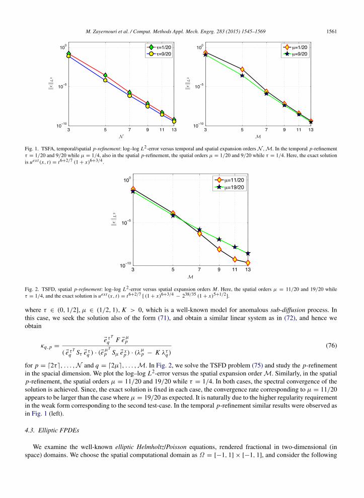
In Fig. 1, we examine the TSFA problem (70) and study the p-refinement in both the temporal (left) and thespatial (right) dimensions. To demonstrate the spectral convergence of the PG spectral method, we plot the log–logL2-error versus temporal and spatial expansion orders N ,M. In the temporal p-refinement τ = 1/20 and 9/20 whileµ = 1/4; also in the spatial p-refinement, the spatial orders µ = 1/20 and 9/20 while τ = 1/4. In this test, we setthe simulation time to T = 1, while the exact solution is uext (x, t) = t6+2/7 (1 + x)6+3/4.

4.2. Parabolic FPDEs

First, we consider the following parabolic Time- and Space-Fractional Diffusion (TSFD) equation

0 D2τt u(x, t) = K −1 D2µ

x u(x, t)+ f (x, t), (x, t) ∈ [0, T ] × [−1, 1], (75)

u(x, 0) = 0,

u(±1, t) = 0,


Fig. 1. TSFA, temporal/spatial p-refinement: log–log L2-error versus temporal and spatial expansion orders N ,M. In the temporal p-refinementτ = 1/20 and 9/20 while µ = 1/4, also in the spatial p-refinement, the spatial orders µ = 1/20 and 9/20 while τ = 1/4. Here, the exact solutionis uext (x, t) = t6+2/7 (1 + x)6+3/4.

Fig. 2. TSFD, spatial p-refinement: log–log L2-error versus spatial expansion orders M . Here, the spatial orders µ = 11/20 and 19/20 whileτ = 1/4, and the exact solution is uext (x, t) = t6+2/7

[ (1 + x)6+3/4− 238/35 (1 + x)5+1/2

].

where τ ∈ (0, 1/2], µ ∈ (1/2, 1), K > 0, which is a well-known model for anomalous sub-diffusion process. Inthis case, we seek the solution also of the form (71), and obtain a similar linear system as in (72), and hence weobtain

κq,p =e τ

T

q F eµp

( e τ Tq Sτ e τq ) · (eµ

T

p Sµ e xp ) · (λ

µp − K λτq)

(76)

for p = ⌈2τ⌉, . . . ,N and q = ⌈2µ⌉, . . . ,M. In Fig. 2, we solve the TSFD problem (75) and study the p-refinementin the spacial dimension. We plot the log–log L2-error versus the spatial expansion order M. Similarly, in the spatialp-refinement, the spatial orders µ = 11/20 and 19/20 while τ = 1/4. In both cases, the spectral convergence of thesolution is achieved. Since, the exact solution is fixed in each case, the convergence rate corresponding to µ = 11/20appears to be larger than the case where µ = 19/20 as expected. It is naturally due to the higher regularity requirementin the weak form corresponding to the second test-case. In the temporal p-refinement similar results were observed asin Fig. 1 (left).

4.3. Elliptic FPDEs

We examine the well-known elliptic Helmholtz/Poisson equations, rendered fractional in two-dimensional (inspace) domains. We choose the spatial computational domain as Ω = [−1, 1] × [−1, 1], and consider the following


Fig. 3. Space-fractional Helmholtz problem with γ = 1, spatial p-refinement in x-dimension: log–log L2-error versus spatial expansion ordersMx1 . Here, the spatial orders are µ1 = 11/20 and 19/20 while µ2 = 15/20, is kept constant. The exact solution is uext (x1, x2) =

[ (1 + x1)6+3/4

− 25/4 (1 + x1)5+1/2

][ (1 + x2)6+4/9

− 273/63 (1 + x2)5+2/7

]. A similar convergence curve is achieved in the p-refinementperformed in the y-dimension, also for the case of γ = 0.

problem

−1 D2µ1x1

u(x1, x2)+ −1 D2µ2x2

u(x1, x2)+ γ u(x1, x2) = f (x1, x2), in Ω , (77)

u(x1, x2) = 0, on ∂Ω

where γ > 0, µ1, µ2 ∈ (1/2, 1), which reduces to the Space-Fractional Poisson equation when γ = 0. Here, wepresent a general scheme in addition to a linear fast solver for both problems.

We then seek the solution to (77) in terms of a linear combination of elements in UN in absence of the time-basis,consisting of only two dimensions of the form

uN (x1, x2) =

M1m1=2

M2m2=2

um1,m2

φ µ1

m1 ξ1

(x1)

φ µ2

m2 ξ2

(x2), (78)

for which we represent the unknown coefficient matrix U in terms of the spatial eigenvectors as

U =

M1p1=2

M2p2=2

κp1,p2 eµ1p1

eµ2T

p2, (79)

where

κp1,p2 =eµ1

T

p1 G eµ2p2

(eµ1T

p1 Sµ1 eµ1p1 ) · ( eµ2

T

p2 Sµ2 eµ2p2 ) · ( λ

µ1p1 + λ

µ2p2 + γ λ

µ1p1 λ

x2p2 )

. (80)

In Fig. 3, we solve the fractional Helmholtz problem (77) and study the p-refinement in the spacial x1-dimension.To demonstrate the spectral convergence of the fast FPDE solver, we plot the log–log L2-error versus the spatial ex-pansion order Mx1 . The spatial ordersµ1 = 11/20 and 19/20 whileµ2 = 15/20. Similar to the spatial p-convergencein Fig. 2, the convergence rate corresponding to µ1 = 11/20 appears to be larger than the case where µ2 = 19/20.We observe a similar p-refinement in the x2-dimension as well.

4.4. Higher-dimensional FPDEs

Next, we employ our PG method and the fast solver in even higher dimensional problems to exhibit the generalityand efficiency of the scheme. In Table 1, the convergence results and CPU time of the unified PG spectral method


Table 1Convergence study and CPU time of the unified PG spectral method employed in the time- and

space-fractional advection equation (TSFA) 0 D2τt u +

dj=1 [−1 D

2µ jx j u] = f , where 2τ = 2µ j =

1/2, j = 1, 2, . . . , d , subject to homogeneous Dirichlet boundary conditions in four-dimensional(4-D), six-dimensional (6-D), and ten-dimensional (10-D) space–time hypercube domains, whereD = 1+d . The error is measured by the essential norm ∥ϵ∥L∞ = ∥u−uext

∥L∞/∥uext∥L∞ , which

is normalized by the essential norm of the exact solution uext (t, x) = [td

j=1(1 + x j )]2+2/5,

where t ∈ [0, 1] and x ∈ [−1, 1]d . The CPU time (seconds) is obtained on a Intel (Xeon X5550)

2.67 GHz processor. In each step, we uniformly increase the bases order by one in all dimensions.

N = M1 = · · · = Md ∥ϵ∥L∞ CPU Time (s)

4-D TSFA2 0.576869 0.0063333 0.034706 0.0159974 0.003990 0.0419945 0.0009071 0.105984

6-D TSFA2 0.741056 0.0147483 0.055171 0.1343134 0.006578 0.8212085 0.001525 3.546791

10-D TSFA2 0.903357 0.2889563 0.095305 18.453204 0.0119229 370.1 (≈6 min)5 0.0028102 3332.4 (≈55 min)

in higher-dimensional problems are examined. Particularly, we employ this scheme to solve the time- and space-fractional advection equation (TSFA)

0 D2τt u + −1 D2µ1

x1u + −1 D2µ2

x2u + · · · + −1 D2µd

xdu = f,

where 2τ = 2µ j = 1/2, subject to homogeneous Dirichlet boundary conditions in a four-dimensional (4-D), six-dimensional (6-D), and ten-dimensional (10-D) space–time hypercube domains. The error is measured by the essentialnorm ∥ϵ∥L∞ = ∥u − uext

∥L∞/∥uext∥L∞ , which is stronger than the L2-norm and is normalized by the essential norm

of the exact solution uext (t, x) = [td

j=1(1 + x j )]2+2/5 for the sake of consistency. The CPU time (seconds) is

measured on a single core Intel (Xeon X5550) 2.67 GHz processor. In each step of the p-refinement, we uniformlyincrease the bases order by one in all dimensions. All the computations are performed in Mathematica 8. Thesesimulations highlight that the unified PG spectral method is efficient even for a 10-D problem run on a PC in less thanan hour!

4.5. Time-integration when 2τ = 1

We recall that our unified PG spectral method works equally well when the temporal time-derivative order 2τ = 1.In general, a first-order in time PDE/FPDE reads

∂u

∂t= F(u; t, x1, . . . , xd), (81)

where the operator F(u; t, x1, . . . , xd) is given as

F(u; t, x1, . . . , xd) = f (t, x1, . . . , xd)−

dj=1

c j [ a j D2µ jx j u ] + γ u,

in view of (8). Here, we regard the PG method as an alternative scheme for spectrally accurate time-integrationfor a general F(u; t, x1, . . . , xd), rather than utilizing existing algebraically accurate methods, including multi-step


Table 2

Time-Integration when 2τ = 1: ∂u/∂t +3

j=1 [−1 D2µ jx j u] = f in Ω ⊂ R1+3, where t ∈ [0, 1]

and x j ∈ [−1, 1], j = 1, 2, 3. Here, we set µ j = 1/2 to fully recover the standard time-dependentadvection equation in three-dimensional spatial domain. However, in general µ j ∈ (0, 1). The erroris measured by the essential norm ∥ϵ∥L∞ = ∥u − uext

∥L∞/∥uext∥L∞ , which is normalized by

the essential norm of the exact solution is uext (t, x) = [t3

j=1(1 + x j )]6+2/5. The CPU time

(seconds) is obtained on a Intel (Xeon X5550) 2.67 GHz processor. In each step, we uniformlyincrease the bases order by one in all dimensions.

N = M1 = M2 = M3 ∥ϵ∥L∞ CPU Time (s)

Integer-order time-integration3 0.6225970 0.0519925 0.0336570 0.3529477 1.34 × 10−5 1.97379 1.06 × 10−7 3.7894

11 3.52 × 10−9 9.736513 2.54 × 10−10 21.472

methods such as the Adams family and stiffly-stable schemes, also multi-stage approaches such as the Runge–Kuttamethod.

The idea of employing the PG spectral method when 2τ = 1 is simply based on the useful property (5) by which afull first-order derivative d/dt can be decomposed into a product of the sequential ( 1

2 )th order derivatives 0 D1/2t 0 D1/2

t ,a result that is not valid in the standard (integer-order) calculus. Hence, by virtue of the fractional integration-by-parts,such a decomposition artificially induces non-locality to the temporal term in the corresponding weak form. Therefore,it provides an appropriate framework for global (spectral) treatment of the temporal term using our unified PG spectralmethod. To this end, we carry out the time-integration when 2τ = 1 in the following FPDE

∂u/∂t +

3j=1

−1 D2µ jx j u = f

in Ω ⊂ R1+3, where in general µ j ∈ (0, 1). Here, we set µ j = 1/2 for simplicity, which recovers the standardtime-dependent advection equation in three-dimensional spatial domain.

In Table 2, we again measure the error by the normalized essential norm, where the exact solution is uext (t, x) =

[t3

j=1(1 + x j )]6+2/5, where t ∈ [0, 1] and x j ∈ [−1, 1], j = 1, 2, 3. Similar to the previous case, the CPU time

(seconds) is obtained on a single-core Intel (Xeon X5550) 2.67 GHz processor, where we uniformly increase the basesorder by one in all dimensions in each step. In these simulations, we globally treat the time-axis in addition to otherspatial dimensions. The CPU time and the spectral convergence strongly highlight the efficiency of our approach,where a 4-D problem (i.e., 1-D in time and 3-D in space) can be highly accurately solved in a fraction of minute!

5. Summary and discussion

We developed a unified and spectrally accurate Petrov–Galerkin (PG) spectral method for a weak formulation of

the general linear FPDE of the form 0 D2τt u+

dj=1 cx j [ a j D2µ j

x j u ]+γ u = f, τ, µ j ∈ (0, 1), in a (1+d)-dimensionalspace–time domain subject to Dirichlet initial and boundary conditions. We demonstrated that this scheme performswell for the whole family of linear hyperbolic-, parabolic- and elli ptic-like equations with the same ease. Wedeveloped our PG method based on a new spectral theory for fractional Sturm–Liouville problems (FSLPs), recentlyintroduced in [42]. In the present method, all the aforementioned matrices are constructed exactly and efficiently. Weadditionally performed the stability analysis (in 1-D) and the corresponding convergence study of the scheme (in multi-D). Moreover, we formulated a new general fast linear solver based on the eigenpairs of the corresponding temporaland spatial mass matrices with respect to the stiffness matrices, which significantly reduces the computational cost inhigher-dimensional problems e.g., (1 + 3), (1 + 5) and (1 + 9)-dimensional FPDEs.

In the p-refinement tests performed in the aforementioned problems, we kept the fractional order to be the middle-value (either 1/2 or 3/2) in the fixed direction, and we examined some limit fractional orders in the other direction.


However, we numerically observe that if the fixed fractional order is taken to be closer to the limit values (i.e., either0 or 1), the mode of spectral convergence remains unchanged but we achieve a different rate of convergence to beverified in our future theoretical analysis.

Alternating Direction Implicit (ADI) methods (see e.g., [49]) are another way of solving space-fractional FPDEsin higher dimensional problems. In this approach, a one-dimensional space-fractional FPDE solver with a low-order (finite-difference) time integrator can be employed to solve 2-D or 3-D problems. However, we note that ADInaturally cannot treat time- and space-fractional FPDEs. Moreover, the temporal rate of convergence in this approachis algebraic in contrast to the high accuracy in the spatial discretizations. Hence, the computational complexity of thisapproach becomes exceedingly large in higher-dimensional FPDEs.

In practice, the enforcement of periodic boundary conditions to FPDEs is not possible since it is not clear howto define history (memory) for a periodic function. Moreover, we note that Riemann–Liouville fractional derivativesin time/space only allow us to impose homogeneous initial/boundary conditions to the corresponding FPDEs to bewell-posed. However, we note that our PG spectral method is also applicable in such problems in the followingmanner. When inhomogeneous Dirichlet conditions are enforced, the corresponding derivatives are usually replacedby Caputo fractional derivatives. We illustrate such a treatment in the following model problem posed subject to aninhomogeneous initial condition:

C0 D2τ

t u = −1 D2µx u + f (x, t), (82)

u(x, 0) = g(x),

u(±1, t) = 0,

in which 2µ ∈ (1, 2), g(x) ∈ C0([−1, 1]), and C0 D2τ

t (·) denotes the Caputo fractional derivative of order 2τ ∈ (0, 1),which is defined via interchanging the order of differentiation and integration in (3), see e.g., [2]. Now, we defineU (x, t) = u(x, t) − g(x), and taking into account that C

0 D2τt g(x) ≡ 0. Then, by substituting u = U + g into (82)

and noting that C0 D2τ

t U = 0 D2τt U due to the homogeneity of U (x, 0), we obtain the transformed problem as

0 D2τt U = −1 D2µ

x U + f (x, t), (83)

U (x, 0) = 0,

U (±1, t) = 0,

in which f (x, t) = f (x, t)+ −1 D2µx g(x). Therefore, we can treat such inhomogeneous conditions by our unified PG

spectral method through homogenizing the problem and modifying the forcing term on the right-hand side. The sameapproach applies to inhomogeneous boundary conditions.

Although the proposed unified PG method enjoys the high accuracy of the discretization in time and space inaddition to its efficiency in solving higher-dimensional problems, treating FPDEs in complex geometries still remainsa great challenge to be addressed in our future works. Moreover, special care should be taken when the FPDE of theinterest is associated with variable coefficients and/or non-linearity. In [44], we have employed the fractional basesto construct a new class of fractional Lagrange interpolants i.e., fractional nodal rather than modal basis functionspresented here, to develop efficient and spectrally accurate collocation methods for a variety of FODEs and FPDEsincluding non-linear space-fractional Burgers’ equation.

Acknowledgments

This work was supported by the Collaboratory on Mathematics for Mesoscopic Modeling of Materials (CM4) atPNNL funded by the Department of Energy Grant #: DE-SC0009247, by OSD/MURI Grant #: FA9550-09-1-0613and by NSF/DMS Grant #: DMS-1216437.

Appendix

Theorem A.1. The temporal stiffness matrix Sτ corresponding to the time-fractional order τ ∈ (0, 1) is a diagonalN × N matrix, whose entries are explicitly given as

Sτ n,n = σn σn

Γ (n + τ)

Γ (n)

2 2T

2τ−1 22n − 1

, n = 1, 2, . . . , N .


Proof. By the PG projection, the (r, n)th entry of the stiffness matrix, r, n = 1, 2, . . . ,N , is defined as

Sτ r,n =

T

0t Dτ

T

Ψ τ

r η(t)0 Dτ

t

ψτn η

(t) dt. (84)

Following [42], we obtain the Riemann–Liouville left-sided time-fractional derivative of the temporal basis as

0 Dτt

ψτn η

(t) = σn

2T

τ Γ (n + τ)

Γ (n)Pn−1( 2t/T − 1 ), (85)

where Pn−1( 2t/T − 1 ) represents the (n − 1)th order Legendre polynomial in t ∈ [0, T ]. Also, we obtain the right-sided time-fractional derivative of the temporal basis again following [42] as

t DτT

Ψ τ

r η(t) = σr

2T

τ Γ (r + τ)

Γ (r)Pr−1( 2t/T − 1 ). (86)

Now, by plugging (85) and (86) into (84), we obtain

Sτ r,n = σr σnΓ (r + τ)

Γ (r)Γ (n + τ)

Γ (n)

2T

2τ T

0Pr−1(x(t)) Pn−1(x(t)) dt

= σr σnΓ (r + τ)

Γ (r)Γ (n + τ)

Γ (n)

2T

2τ−1 1

−1Pr−1(x) Pn−1(x) dx

= σr σnΓ (r + τ)

Γ (r)Γ (n + τ)

Γ (n)

2T

2τ−1 22n − 1

δrn, (87)

by the orthogonality of the Legendre polynomials, where δrn is the Kronecker delta functions.

Theorem A.2. (I) If µ j ∈ (0, 1/2], the spatial stiffness matrix Sµ j is a diagonal M j × M j matrix, whose entriesare explicitly given as

Sµ j k,k = σk σk

Γ (k + µ j )

Γ (k)

2 2L j

2µ j −1 22k − 1

, k = 1, 2, . . . ,M j .

(II) If µ j ∈ (1/2, 1), Sµ j is a symmetric tridiagonal (M j − 1)× (M j − 1) with entries, explicitly given as

Sµ j k,m = bk am

Γ (k + µ j )

Γ (k)

2 2L j

2µ j −1 22k − 1

δk,m − ϵ

µ jm δk,m−1

+ ϵ

µ jk bk am

Γ (k − 1 + µ j )

Γ (k − 1)

2 2L j

2µ j −1 22k − 3

δk−1,m − ϵ

µ jm δk−1,m−1

,

k,m = 2, 3, . . . ,M j and L j = b j − a j .

Proof. The first part, when µ j ∈ (0, 1/2] is similar to the proof in Theorem A.1, however, carried out on the interval

[a j , b j ] rather than [0, T ]. Here, the µ j th order left-sided Riemann–Liouville fractional derivative ofφµ jm j ξ j

(x j )

is given following [42] as

a j D µ jx j

φµ jm ξ j

(x j ) =

Bµ jm Pm−1

ξ(x j )

, µ j ∈ (0, 1/2],

Bµ jm Pm−1

ξ(x j )

− C

µ jm Pm−2

ξ(x j )

, µ j ∈ (1/2, 1),

(88)

for m = ⌈2µ j⌉, . . . ,M j in the j th spatial dimension, where the coefficient Bµ jm j = σm (2/L j )

2µ j Γ (m + µ j )/Γ (m)and C

µ jm = σm (2/L j )

2µ j ϵµ jm Γ (m − 1 + µ j )/Γ (m − 1); in addition, the µ j th order left-sided Riemann–Liouville

fractional derivative ofΦµ jm ξ j

(x j ) is obtained as

x j D µ jb j

Φµ jm ξ j

(x j ) =

Bµ jk Pk−1

ξ(x j )

, µ j ∈ (0, 1/2],

Bµ jk Pk−1

ξ(x j )

− Cµ j

k Pk−2

ξ(x j )

, µ j ∈ (1/2, 1),

(89)


for k = ⌈2µ j⌉, . . . ,M j in the j th spatial dimension, in which we set the coefficient Bµ jk = σk (2/L j )

2µ j Γ (k +

µ j )/Γ (k) and Cµ jk = σk (2/L j )

2µ j ϵµ jk Γ (k − 1 + µ j )/Γ (k − 1).

For the second part, when µ j ∈ (1/2, 1), the (k,m)th entry of Sµ j is

Sµ j k,m =

b j

a j

x j Dµ jb j

Φµ jk ξ j

(x j )a j Dµ j

x j

φµ jm ξ j

(x j )dx j .

Next, by virtue of (88) and (89), also by an affine mapping from [a j , b j ] to the standard interval [−1, 1], we obtain

Sµ j k,m =

L j

2

1

−1

Bµ jm Pm−1( ξ j )− C

µ jm Pm−2( ξ j )

Bµ j

k Pk−1( ξ j )− Cµ jk Pk−2( ξ j )

dξ j .

Hence, by the orthogonality of the Legendre polynomials we obtain

Sµ j k,m =

L j

2

Bµ jm Bµ j

k2

2k − 1δk,m − C

µ jm Bµ j

k2

2k − 1δk,m−1

+ Bµ jm Cµ j

k2

2k − 3δk−1,m − C

µ jm Cµ j

k2

2k − 3δk−1,m−1

,

which completes the proof, while the symmetry of the stiffness matrix can be easily checked.

Theorem A.3. The temporal and the spatial mass matrices Mτ as well as Mµ j are symmetric. Moreover, theirentries can be computed exactly by employing a Gauss–Lobatto–Jacobi (GLJ) rule with respect to the weight function(1 − ξ)α(1 + ξ)α, ξ ∈ [−1, 1], where α = τ/2 in the temporal and α = µ j for the spatial case.

Proof. The entries of Mτ in our PG spectral method are defined as

Mτ r,n =

T

0

Ψ τ

r η(t)

ψµt

m η(t)dt,

which be computed exactly as

Mτ r,n = σr σn

2T

τ T

0tτ (T − t)τ Pτ,−τr−1 ( η(t) ) P−τ, τ

n−1 ( η(t) ) dt

= σr σnT

2

1

−1(1 − η)τ (1 + η)τ Pτ,−τr−1 (η) P−τ, τ

n−1 (η)dη

= σr σnT

2

Qq=1

wq Pτ,−τr−1 (ηq)P−τ, τn−1 (ηq), (90)

in which Q ≥ N + 2 represents the minimum number of GLJ quadrature points ηqQq=1, associated with the weigh

function (1 − η)τ (1 + η)τ , for exact quadrature, and wqQq=1 are the corresponding quadrature weights. From the

exact discrete rule, recalling the definition of σn and σr , employing the property of the Jacobi polynomials wherePα,βn (−x) = (−1)n Pβ,αn (x), moreover, noting that ηq

Qq=1 and wq

Qq=1 are symmetric with respect to the reference

point, it is easy to show that Mτ r,n = Mτ n,r .The spatial mass matrix Mµ j , when µ j ∈ (0, 1/2], is also M j × M j , whose entries are computed similarly as

Mµ j k,m = σk σmL j

2

Qq=1

wq Pµ j ,−µ jk−1 (ξq)P

−µ j , µ jm−1 (ξq), (91)

in which Q ≥ M j + 2 represents the minimum number of GLJ quadrature points ξqQq=1, associated with the weigh

function (1 − ξ)µ j (1 + ξ)µ j , for exact quadrature. We can also show that Mµ j is symmetric and that the GJL rule isexact when Q ≥ M j + 2.


Finally, when µ j ∈ (1/2, 1), the spatial mass matrix Mµ j , becomes (M j − 1) × (M j − 1), whose entries arecomputed exactly as

Mµ j k,m =

b j

a j

Φµ j /2k ξ

(x j )

φµ j /2m ξ

(x j )dx j

= σk j σm j

1

−1

(2)P µ jk j( ξ(x j ) )

(1)P µxm ( ξ(x j ) ) dx j

− ϵµxm

1

−1

(2)P µ jk j( ξ(x j ) )

(1)P µ jm j −1( ξ(x j ) ) dx j

+ ϵµxk

1

−1

(2)P µ jk j −1( ξ(x j ) )

(1)P µ jm j ( ξ(x j ) ) dx j

− ϵµ jk jϵµ jm j

1

−1

(2)P µ jk j −1( ξ(x j ) )

(1)P µ jm j −1( ξ(x j ) )dx j

,

where we note that all the above integrations share the same weight function by construction. Hence, we obtain

Mµ j k,m = σk j σm j

L j

2

1

−1(1 − ξ)µ j (1 + ξ)µ j

Pµ j ,−µ jk−1 (ξ) P

−µ j , µ jm−1 (ξ)

− ϵµxm P

µ j ,−µ jk−1 (ξ) P

−µ j , µ jm−2 (ξ)+ ϵ

µxk P

µ j ,−µ jk−2 (ξ) P

−µ j , µ jm−1 (ξ)

− ϵµ jk jϵµ jm j P

µ j ,−µ jk−2 (ξ) P

−µ j , µ jm−2 (ξ)

dx j

which leads to the following exact GLJ rule

Mµ j k,m = σk jσm j

L j

2

Qq=1

wq

Pµ j ,−µ jk−1 (ξq) P

−µ j , µ jm−1 (ξq)− ϵµx

m Pµ j ,−µ jk−1 (ξq) P

−µ j , µ jm−2 (ξq)

+ ϵµxk P

µ j ,−µ jk−2 (ξq) P

−µ j , µ jm−1 (ξq)− ϵ

µ jk jϵµ jm j P

µ j ,−µ jk−2 (ξq) P

−µ j , µ jm−2 (ξq)

, (92)

which is also exact when Q ≥ M j + 2, and the same argument on the symmetry of the matrix applies here.

References

[1] K.S. Miller, B. Ross, An Introduction to the Fractional Calculus and Fractional Differential Equations, John Wiley and Sons, Inc., New York,NY, 1993.

[2] I. Podlubny, Fractional Differential Equations, Academic Press, San Diego, CA, USA, 1999.[3] B.J. West, M. Bologna, P. Grigolini, Physics of Fractal Operators, Springer Verlag, New York, NY, 2003.[4] F. Mainardi, Fractional Calculus and Waves in Linear Viscoelasticity: An Introduction to Mathematical Models, Imperial College Press, 2010.[5] D.A. Benson, S.W. Wheatcraft, M.M. Meerschaert, Application of a fractional advection–dispersion equation, Water Resour. Res. 36 (6)

(2000) 1403–1412.[6] W. Chester, Resonant oscillations in closed tubes, J. Fluid Mech. 18 (1) (1964) 44–64.[7] J.J. Keller, Propagation of simple non-linear waves in gas filled tubes with friction, Z. Angew. Math. Phys. 32 (2) (1981) 170–181.[8] N. Sugimoto, T. Kakutani, Generalized Burgers’ equation for nonlinear viscoelastic waves, Wave Motion 7 (5) (1985) 447–458.[9] R.L. Magin, Fractional Calculus in Bioengineering, Begell House Inc., Redding, CT, 2006.

[10] J.P. Bouchaud, A. Georges, Anomalous diffusion in disordered media: statistical mechanisms, models and physical applications, Phys. Rep.195 (4) (1990) 127–293.

[11] R. Metzler, J. Klafter, The random walk’s guide to anomalous diffusion: a fractional dynamics approach, Phys. Rep. 339 (1) (2000) 1–77.[12] R. Klages, G. Radons, I.M. Sokolov, Anomalous Transport: Foundations and Applications, Wiley-VCH, 2008.[13] B. Henry, S. Wearne, Fractional reaction–diffusion, Physica A 276 (3) (2000) 448–455.[14] N. Sugimoto, Burgers equation with a fractional derivative; hereditary effects on nonlinear acoustic waves, J. Fluid Mech. 225 (631–653)

(1991) 4.[15] G. Autuori, P. Pucci, Elliptic problems involving the fractional Laplacian in RN, J. Differential Equations 255 (8) (2013) 2340–2362.[16] B. Gustafsson, H.O. Kreiss, J. Oliger, Time Dependent Problems and Difference Methods, Vol. 67, Wiley, New York, 1995.[17] J.S. Hesthaven, S. Gottlieb, D. Gottlieb, Spectral Methods for Time-dependent Problems, Vol. 21, Cambridge University Press, 2007.[18] O.C. Zienkiewicz, R.L. Taylor, J.Z. Zhu, The Finite Element Method: its Basis and Fundamentals, Butterworth-Heinemann, 2005.[19] G.E. Karniadakis, S.J. Sherwin, Spectral/HP Element Methods for CFD, second ed., Oxford University Press, 2005.

http://refhub.elsevier.com/S0045-7825(14)00421-6/sbref1




















[20] C. Lubich, On the stability of linear multistep methods for Volterra convolution equations, IMA J. Numer. Anal. 3 (4) (1983) 439–465.[21] C. Lubich, Discretized fractional calculus, SIAM J. Math. Anal. 17 (3) (1986) 704–719.[22] J.M. Sanz-Serna, A numerical method for a partial integro-differential equation, SIAM J. Numer. Anal. 25 (2) (1988) 319–327.[23] T. Langlands, B. Henry, The accuracy and stability of an implicit solution method for the fractional diffusion equation, J. Comput. Phys. 205

(2) (2005) 719–736.[24] Z. Sun, X. Wu, A fully discrete difference scheme for a diffusion-wave system, Appl. Numer. Math. 56 (2) (2006) 193–209.[25] Y. Lin, C. Xu, Finite difference/spectral approximations for the time-fractional diffusion equation, J. Comput. Phys. 225 (2) (2007) 1533–1552.[26] J. Cao, C. Xu, A high order schema for the numerical solution of the fractional ordinary differential equations, J. Comput. Phys. 238 (1)

(2013) 154–168.[27] L. Blank, Numerical treatment of differential equations of fractional order, Citeseer (1996).[28] E.A. Rawashdeh, Numerical solution of fractional integro-differential equations by collocation method, Appl. Math. Comput. 176 (1) (2006)

1–6.[29] X. Li, C. Xu, A space–time spectral method for the time fractional diffusion equation, SIAM J. Numer. Anal. 47 (3) (2009) 2108–2131.[30] X. Li, C. Xu, Existence and uniqueness of the weak solution of the space–time fractional diffusion equation and a spectral method

approximation, Commun. Comput. Phys. 8 (5) (2010) 1016.[31] G.J. Fix, J.P. Roop, Least squares finite-element solution of a fractional order two-point boundary value problem, Comput. Math. Appl. 48 (7)

(2004) 1017–1033.[32] M.M. Khader, On the numerical solutions for the fractional diffusion equation, Commun. Nonlinear Sci. Numer. Simul. 16 (6) (2011)

2535–2542.[33] C. Piret, E. Hanert, A radial basis functions method for fractional diffusion equations, J. Comput. Phys. (2012) 71–81.[34] E. Doha, A. Bhrawy, S. Ezz-Eldien, A Chebyshev spectral method based on operational matrix for initial and boundary value problems of

fractional order, Comput. Math. Appl. 62 (5) (2011) 2364–2373.[35] A.H. Bhrawy, M.M. Al-Shomrani, A shifted Legendre spectral method for fractional-order multi-point boundary value problems, Adv.

Difference Equ. 2012 (1) (2012) 1–19.[36] M. Maleki, I. Hashim, M.T. Kajani, S. Abbasbandy, An adaptive pseudospectral method for fractional order boundary value problems,

in: Abstract and Applied Analysis, vol. 2012, Hindawi Publishing Corporation, 2012.[37] D. Baleanu, A. Bhrawy, T. Taha, Two efficient generalized Laguerre spectral algorithms for fractional initial value problems, in: Abstract and

Applied Analysis, vol. 2013, Hindawi Publishing Corporation, 2013.[38] A. Bhrawy, M. Alghamdia, A New Legendre spectral Galerkin and pseudo-spectral approximations for fractional initial value problems, 2013.[39] Q. Xu, J. Hesthaven, Stable multi-domain spectral penalty methods for fractional partial differential equations, J. Comput. Phys. 257 (2014)

241–258.[40] M. Zayernouri, G.E. Karniadakis, Exponentially accurate spectral and spectral element methods for fractional ODEs, J. Comput. Phys. 257

(2014) 460–480.[41] M. Zayernouri, W. Cao, Z. Zhang, G.E. Karniadakis, Spectral and discontinuous spectral element methods for fractional delay equations,

SIAM J. Sci. Comput. 36 (6) (2014) B904–B929.[42] M. Zayernouri, G.E. Karniadakis, Fractional Sturm–Liouville eigen-problems: theory and numerical approximation, J. Comput. Phys. 252

(2013) 495–517.[43] M. Zayernouri, G.E. Karniadakis, Discontinuous spectral element methods for time- and space-fractional advection equations, SIAM J. Sci.

Comput. 36 (4) (2014) B684–B707.[44] M. Zayernouri, G.E. Karniadakis, Fractional spectral collocation method, SIAM J. Sci. Comput. 36 (1) (2014) A40–A62.[45] M. Zayernouri, G.E. Karniadakis, Fractional spectral collocation methods for linear and nonlinear variable order FPDEs, J. Comput. Phys.

(2014). A special issue on FPDEs, in press.[46] J.P. Roop, Variational solution of the fractional advection–dispersion equation (Ph.D. dissertation), Clemson University, Department of

Mathematical Sciences, 2004.[47] J.P. Roop, Computational aspects of FEM approximation of fractional advection dispersion equations on bounded domains in R2, J. Comput.

Appl. Math. 193 (1) (2006) 243–268.[48] A. Ern, Theory and Practice of Finite Elements, Vol. 159, Springer, 2004.[49] G.E. Karniadakis, R.M. Kirby II, Parallel Scientific Computing in C++ and MPI: a Seamless Approach to Parallel Algorithms and their

Implementation, Cambridge University Press, 2003.






























Date post:	01-May-2020
Category:	Documents
Upload:	others
View:	6 times
Download:	0 times

A unified Petrov–Galerkin spectral method for fractional PDEs€¦ · Petrov–Galerkin (DPG) and...

Documents