A Unified Theory of Bond andCurrency Markets

Andrey Ermolov

Columbia Business School

April 24, 2014

1 / 41

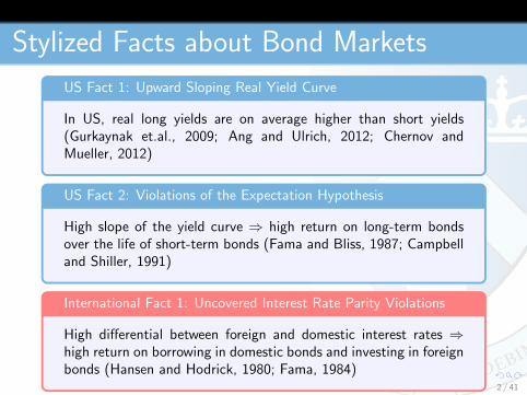
Stylized Facts about Bond Markets

US Fact 1: Upward Sloping Real Yield Curve

In US, real long yields are on average higher than short yields(Gurkaynak et.al., 2009; Ang and Ulrich, 2012; Chernov andMueller, 2012)

US Fact 2: Violations of the Expectation Hypothesis

High slope of the yield curve ⇒ high return on long-term bondsover the life of short-term bonds (Fama and Bliss, 1987; Campbelland Shiller, 1991)

International Fact 1: Uncovered Interest Rate Parity Violations

High differential between foreign and domestic interest rates ⇒high return on borrowing in domestic bonds and investing in foreignbonds (Hansen and Hodrick, 1980; Fama, 1984)

2 / 41

Bermuda Triangle of The TheoreticalBond Markets Literature

US and international bond markets closely integrated,but theoretically difficult to explain them jointly

This paper tries to address this task3 / 41

Agenda

Model

Solutions to the puzzles

Empirical eividence

Calibration

4 / 41

Agenda

ModelSolutions to the puzzles

Empirical evidence

Calibration

5 / 41

Model: Overview

Only real sector

Key components:

Habit utility

Heteroskedastic consumption growth

Contribution: applying model to jointly

explain US and international term

structure6 / 41

Model: Utility

Representative agent

Habit utility: E0

∑∞t=0 β

t (CtHt)1−γ

1−γ

Risk-aversion γ (always assumed >1)

Ct - consumption

Ht - habit: exogeneous standard of living

7 / 41

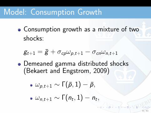
Model: Consumption Growth

Consumption growth as a mixture of two

shocks:

gt+1 = g + σcpωp,t+1 − σcnωn,t+1

Demeaned gamma distributed shocks(Bekaert and Engstrom, 2009)

ωp,t+1 ∼ Γ(p, 1)− p,

ωn,t+1 ∼ Γ(nt, 1)− nt,

8 / 41

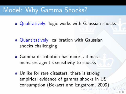
Model: Why Gamma Shocks?

Qualitatively: logic works with Gaussian shocks

Quantitatively: calibration with Gaussianshocks challenging

Gamma distribution has more tail mass:increases agent’s sensitivity to shocks

Unlike for rare disasters, there is strongempirical evidence of gamma shocks in USconsumption (Bekaert and Engstrom, 2009)

9 / 41

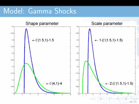
Model: Gamma Shocks

10 / 41

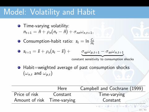
Model: Volatility and Habit

Time-varying volatility:nt+1 = n + ρn(nt − n) + σnnωn,t+1,

Consumption-habit ratio: st = ln Ct

Ht

st+1 = s + ρs(st − s) + σspωp,t+1 − σsnωn,t+1︸ ︷︷ ︸constant sensitivity to consumption shocks

Habit=weighted average of past consumption shocks(ωn,t and ωp,t)

Here Campbell and Cochrane (1999)Price of risk Constant Time-varyingAmount of risk Time-varying Constant

11 / 41

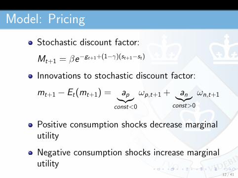
Model: Pricing

Stochastic discount factor:

Mt+1 = βe−gt+1+(1−γ)(st+1−st)

Innovations to stochastic discount factor:

mt+1− Et(mt+1) = ap︸︷︷︸const<0

ωp,t+1 + an︸︷︷︸const>0

ωn,t+1

Positive consumption shocks decrease marginalutility

Negative consumption shocks increase marginalutility

12 / 41

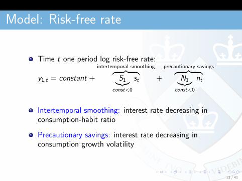
Model: Risk-free rate

Time t one period log risk-free rate:

y1,t = constant +

intertemporal smoothing︷ ︸︸ ︷S1︸︷︷︸

const<0

st +

precautionary savings︷ ︸︸ ︷N1︸︷︷︸

const<0

nt

Intertemporal smoothing: interest rate decreasing inconsumption-habit ratio

Precautionary savings: interest rate decreasing inconsumption growth volatility

13 / 41

Agenda

Model

Solutions to the puzzlesEmpirical evidence

Calibration

14 / 41

Solutions to The Puzzles: Setup 1/3

Time t = 0, 1, 2

At time 0: 1 and 2 period zero-coupon bonds:prices P1,t , P2,t

Yields: y1,t = − lnP1,t and y2,t = −12 lnP2,t

Return on holding 2 period bond over 1 period:R2,t→t+1 =

P1,t+1

P2,t

Taking logs: r2,t→t+1 = −y1,t+1 + 2y2,t

15 / 41

Solutions to The Puzzles: Setup 2/3

Rearranging and taking expectations:y2,t − y1,t︸ ︷︷ ︸

yield curve slope

= 12 Et(y1,t+1 − y1,t)︸ ︷︷ ︸

expected short rate change

+ 12 Et(r2,t→t+1 − y1,t)︸ ︷︷ ︸

risk premium

Holding 2 period bond over 1 period is not risk-free: subject toshort rate risk ⇒ risk premium

Et(r2,t→t+1 − y1,t) ≈ −covt(mt+1, r2,t→t+1) = covt(mt+1, y1,t+1)

16 / 41

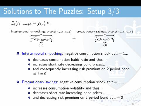
Solutions to The Puzzles: Setup 3/3

Et(r2,t→t+1 − y1,t) ≈intertemporal smoothing, ∝covt(mt+1,st+1)︷ ︸︸ ︷

−S1σsnannt︸ ︷︷ ︸>0

+

precautionary savings, ∝covt(mt+1,nt+1)︷ ︸︸ ︷N1σnnannt︸ ︷︷ ︸

<0

Intertemporal smoothing: negative consumption shock at t = 1...

decreases consumption-habit ratio and thus...increases short rate decreasing bond prices...and consequently increasing risk premium on 2 period bondat t = 0

Precautionary savings: negative consumption shock at t = 1...

increases consumption volatility and thus...decreases short rate increasing bond prices...and decreasing risk premium on 2 period bond at t = 0

17 / 41

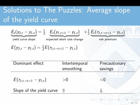
Solutions to The Puzzles: Average slopeof the yield curve

Et(y2,t − y1,t)︸ ︷︷ ︸yield curve slope

= 12

Et(y1,t+1 − y1,t)︸ ︷︷ ︸expected short rate change

+ 12Et(r2,t→t+1 − y1,t)︸ ︷︷ ︸

risk premium

E (y2,t − y1,t) = 12E (r2,t→t+1 − y1,t)

Dominant effect Intertemporalsmoothing

Precautionarysavings

E (r2,t→t+1 − y1,t) >0 <0

Slope of the yield curve ⇑ ⇓

18 / 41

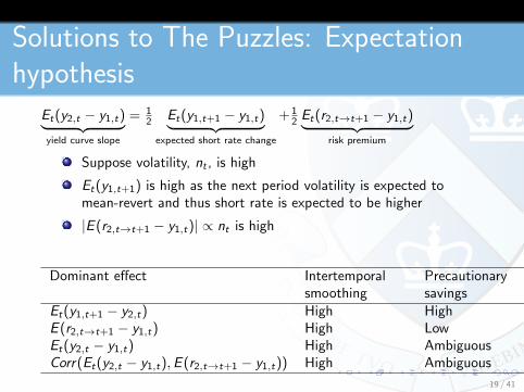
Solutions to The Puzzles: Expectationhypothesis

Et(y2,t − y1,t)︸ ︷︷ ︸yield curve slope

= 12 Et(y1,t+1 − y1,t)︸ ︷︷ ︸

expected short rate change

+ 12 Et(r2,t→t+1 − y1,t)︸ ︷︷ ︸

risk premium

Suppose volatility, nt , is high

Et(y1,t+1) is high as the next period volatility is expected tomean-revert and thus short rate is expected to be higher

|E (r2,t→t+1 − y1,t)| ∝ nt is high

Dominant effect Intertemporalsmoothing

Precautionarysavings

Et(y1,t+1 − y2,t) High HighE (r2,t→t+1 − y1,t) High LowEt(y2,t − y1,t) High AmbiguousCorr(Et(y2,t − y1,t),E (r2,t→t+1 − y1,t)) High Ambiguous

19 / 41

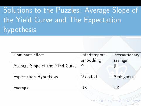
Solutions to the Puzzles: Average Slope ofthe Yield Curve and The Expectationhypothesis

Dominant effect Intertemporalsmoothing

Precautionarysavings

Average Slope of the Yield Curve ⇑ ⇓

Expectation Hypothesis Violated Ambiguous

Example US UK

20 / 41

Solutions to the Puzzles: Longer Horizons

Depending on the parameters, intertemporalsmoothing and precautionary savings will havedifferent strengths at different horizons

Consequently, the yield curve can be upward-or downward-sloping, hump- or U-shaped

Similarly, expectation hypothesis can beviolated at some horizons and not violated atothers

21 / 41

Solutions to The Puzzles: InternationalSetup 1/3

2 symmetric and independent countries: H andL

Each country has its own good

Complete markets=marginal utilities are equalacross countries

No trading frictions or arbitrage opportunities

Exchange rate: Q = H country goodsL country good

22 / 41

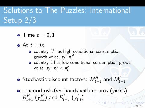
Solutions to The Puzzles: InternationalSetup 2/3

Time t = 0, 1

At t = 0:country H has high conditional consumptiongrowth volatility: nHtcountry L has low conditional consumption growthvolatility: nLt < nHt

Stochastic discount factors: MHt+1 and ML

t+1

1 period risk-free bonds with returns (yields)RHt+1 (yH1,t) and RL

t+1 (yL1,t)

23 / 41

Solutions to The Puzzles: InternationalSetup 3/3

Country L Euler Et(MLt+1R

Lt+1) = 1

Country H Euler for investing in country Lbond Et(M

Ht+1

Qt+1

QtRLt+1) = 1

Complete markets ⇒ unique SDF ⇒ML

t+1 = MHt+1

Qt+1

Qt

Change in log-exchange rate:qt+1 − qt = mL

t+1 −mHt+1

24 / 41

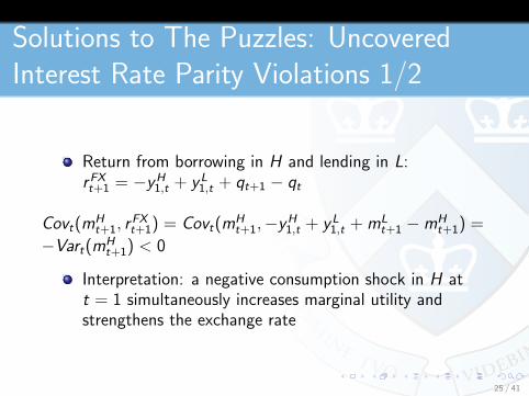
Solutions to The Puzzles: UncoveredInterest Rate Parity Violations 1/2

Return from borrowing in H and lending in L:rFXt+1 = −yH

1,t + yL1,t + qt+1 − qt

Covt(mHt+1, r

FXt+1) = Covt(m

Ht+1,−yH

1,t + yL1,t + mL

t+1 −mHt+1) =

−Vart(mHt+1) < 0

Interpretation: a negative consumption shock in H att = 1 simultaneously increases marginal utility andstrengthens the exchange rate

25 / 41

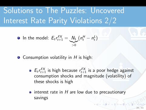
Solutions to The Puzzles: UncoveredInterest Rate Parity Violations 2/2

In the model: EtrFXt+1 = N1︸︷︷︸

>0

(nHt − nLt )

Consumption volatility in H is high:

EtrFXt+1 is high because rFXt+1 is a poor hedge against

consumption shocks and magnitude (volatility) ofthese shocks is high

interest rate in H are low due to precautionarysavings

26 / 41

Agenda

Puzzles

Model

Solutions to the puzzles

Empirical evidenceCalibration

27 / 41

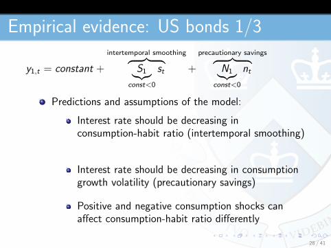
Empirical evidence: US bonds 1/3

y1,t = constant +

intertemporal smoothing︷ ︸︸ ︷S1︸︷︷︸

const<0

st +

precautionary savings︷ ︸︸ ︷N1︸︷︷︸

const<0

nt

Predictions and assumptions of the model:

Interest rate should be decreasing inconsumption-habit ratio (intertemporal smoothing)

Interest rate should be decreasing in consumptiongrowth volatility (precautionary savings)

Positive and negative consumption shocks canaffect consumption-habit ratio differently

28 / 41

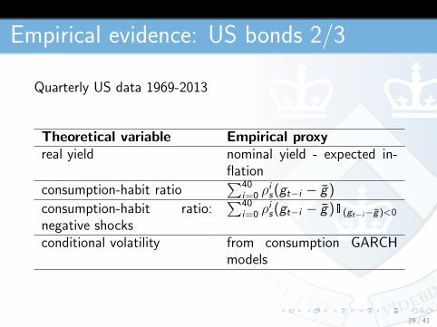
Empirical evidence: US bonds 2/3

Quarterly US data 1969-2013

Theoretical variable Empirical proxyreal yield nominal yield - expected in-

flation

consumption-habit ratio∑40

i=0 ρis(gt−i − g)

consumption-habit ratio:negative shocks

∑40i=0 ρ

is(gt−i − g)1(gt−i−g)<0

conditional volatility from consumption GARCHmodels

29 / 41

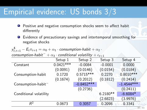
Empirical evidence: US bonds 3/3

Positive and negative consumption shocks seem to affect habitdifferently

Evidence of precautionary savings and intertemporal smoothing fornegative shocks

y$t,t+1 − Etπt+1 = α0 + α1 · consumption-habit + α2 ·consumption-habit− + α3 · conditional volatility + εt+1

Setup 1 Setup 2 Setup 3 Setup 4Constant 0.0421*** -0.0084 -0.0001 0.0000

(0.0091) (0.0146) (0.0154) (0.0184)Consumption-habit 0.1720 0.5715*** 0.2270 0.8010***

(0.1674) (0.2012) (0.1812) (0.2414)Consumption-habit− -0.8452*** -1.4544***

(0.2736) (0.2411)Conditional volatility 6.2180** -6.6084*

(2.6823) (3.9976)R2 0.0673 0.3057 0.2098 0.3341

30 / 41

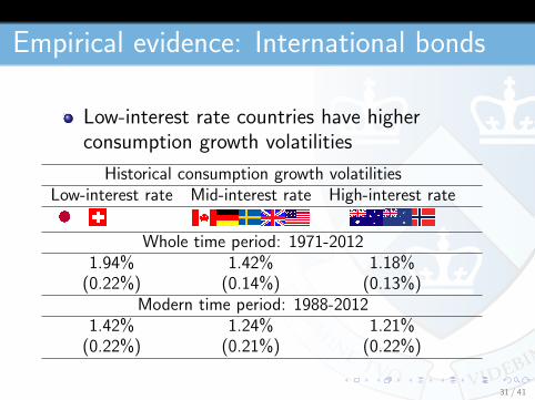
Empirical evidence: International bonds

Low-interest rate countries have higherconsumption growth volatilities

Historical consumption growth volatilitiesLow-interest rate Mid-interest rate High-interest rate

Whole time period: 1971-20121.94% 1.42% 1.18%

(0.22%) (0.14%) (0.13%)Modern time period: 1988-2012

1.42% 1.24% 1.21%(0.22%) (0.21%) (0.22%)

31 / 41

Agenda

Puzzles

Model

Solutions to the puzzles

Empirical evidence

Calibration

32 / 41

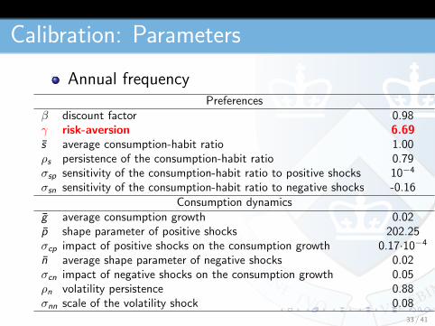
Calibration: Parameters

Annual frequencyPreferences

β discount factor 0.98γ risk-aversion 6.69s average consumption-habit ratio 1.00ρs persistence of the consumption-habit ratio 0.79σsp sensitivity of the consumption-habit ratio to positive shocks 10−4

σsn sensitivity of the consumption-habit ratio to negative shocks -0.16Consumption dynamics

g average consumption growth 0.02p shape parameter of positive shocks 202.25σcp impact of positive shocks on the consumption growth 0.17·10−4

n average shape parameter of negative shocks 0.02σcn impact of negative shocks on the consumption growth 0.05ρn volatility persistence 0.88σnn scale of the volatility shock 0.08

33 / 41

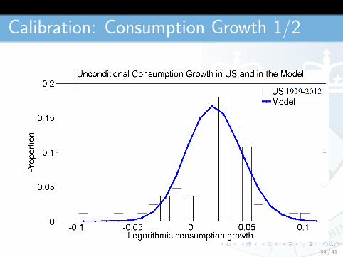
Calibration: Consumption Growth 1/2

34 / 41

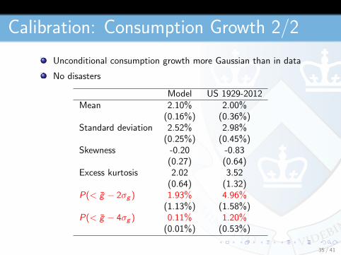
Calibration: Consumption Growth 2/2

Unconditional consumption growth more Gaussian than in data

No disasters

Model US 1929-2012Mean 2.10% 2.00%

(0.16%) (0.36%)Standard deviation 2.52% 2.98%

(0.25%) (0.45%)Skewness -0.20 -0.83

(0.27) (0.64)Excess kurtosis 2.02 3.52

(0.64) (1.32)P(< g − 2σg ) 1.93% 4.96%

(1.13%) (1.58%)P(< g − 4σg ) 0.11% 1.20%

(0.01%) (0.53%)

35 / 41

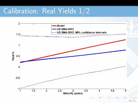
Calibration: Real Yields 1/2

36 / 41

Calibration: Real Yields 2/2

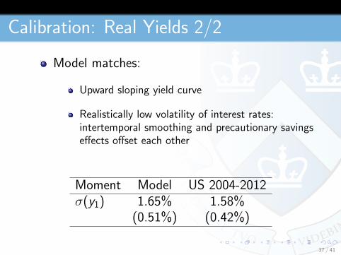
Model matches:

Upward sloping yield curve

Realistically low volatility of interest rates:intertemporal smoothing and precautionary savingseffects offset each other

Moment Model US 2004-2012σ(y1) 1.65% 1.58%

(0.51%) (0.42%)

37 / 41

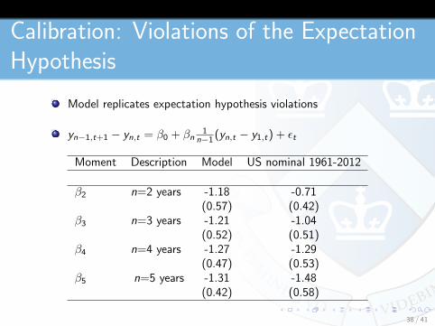
Calibration: Violations of the ExpectationHypothesis

Model replicates expectation hypothesis violations

yn−1,t+1 − yn,t = β0 + βn1

n−1 (yn,t − y1,t) + εt

Moment Description Model US nominal 1961-2012

β2 n=2 years -1.18 -0.71(0.57) (0.42)

β3 n=3 years -1.21 -1.04(0.52) (0.51)

β4 n=4 years -1.27 -1.29(0.47) (0.53)

β5 n=5 years -1.31 -1.48(0.42) (0.58)

38 / 41

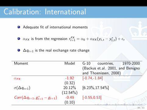
Calibration: International

Adequate fit of international moments

αFX is from the regression rFXt+1 = α0 + αFX (y1,t − y∗1,t) + εt

∆qt+1 is the real exchange rate change

Moment Model G-10 countries, 1970-2000(Backus et.al. 2001, and Benignoand Thoenissen, 2008)

αFX -1.92 [-0.74,-1.84](0.32)

σ(∆qt+1) 20.12% [6.23%,17.54%](12.54%)

Corr(∆qt+1, g∗t+1 − gt+1) -0.49 [-0.55,0.53]

(0.10)39 / 41

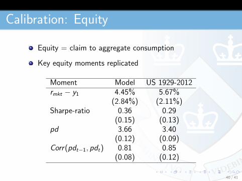
Calibration: Equity

Equity = claim to aggregate consumption

Key equity moments replicated

Moment Model US 1929-2012rmkt − y1 4.45% 5.67%

(2.84%) (2.11%)Sharpe-ratio 0.36 0.29

(0.15) (0.13)pd 3.66 3.40

(0.12) (0.09)Corr(pdt−1, pdt) 0.81 0.85

(0.08) (0.12)

40 / 41

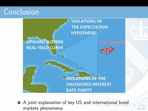
Conclusion

A joint explanation of key US and international bondmarkets phenomena 41 / 41