Page 1
JOTA manuscript No.(will be inserted by the editor)
A Unifying Approach to Robust Convex Infinite
Optimization Duality
Nguyen Dinh · Miguel Angel Goberna ·
Marco Antonio Lopez · Michel Volle
Received: date / Accepted: date
Communicated by Radu Ioan Bot
Abstract This paper considers an uncertain convex optimization problem,
posed in a locally convex decision space with an arbitrary number of un-
Nguyen Dinh
International University, Vietnam National University - HCM City
Chi Minh city, Vietnam; [email protected]
Miguel Angel Goberna
Department of Mathematics, University of Alicante
Alicante, Spain; [email protected]
Marco Antonio Lopez, Corresponding author
Department of Mathematics, University of Alicante
Alicante, Spain; [email protected] ; and
CIAO, Federation University, Ballarat, Australia
Michel Volle
Avignon University
LMA EA2151, Avignon, France; [email protected]
Page 2
2 Nguyen Dinh et al.
certain constraints. To this problem, where the uncertainty only affects the
constraints, we associate a robust (pessimistic) counterpart and several dual
problems. The paper provides corresponding dual variational principles for
the robust counterpart in terms of the closed convexity of different associated
cones.
Keywords Robust convex optimization · Lagrange duality · strong duality ·
robust strong duality · uniform robust strong duality · robust reverse strong
duality.
AMS subject classification 90C25, 46N10, 90C31
1 Introduction
Robust optimization has recently emerged as a useful methodology in the
treatment of uncertain optimization problems. In this paper we consider a
convex optimization problem posed in a locally convex decision space with an
arbitrary number of uncertain constraints. Following the robust approach, we
associate to this uncertain problem a deterministic one called robust coun-
terpart ensuring the feasibility of all possible decisions for any conceivable
scenario. To this problem we associate five different robust dual problems, two
of them already known (the Lagrange dual and the optimistic dual problems),
the remaining three dual problems being apparently new in the literature.
The paper provides robust strong duality theorems for the five duality
pairs guaranteeing the zero-duality gap with attainment of the dual optimal
value which are expressed in terms of the closedness of suitable sets regarding
Page 3
A Unifying Approach to Robust Convex Infinite Optimization Duality 3
the vertical axis. It also provides corresponding stable robust strong duality
theorems guaranteeing robust strong duality for arbitrary linear continuous
perturbations of the objective function which are expressed in terms of the
closedness and convexity of the above sets. Moreover, the paper gives uniform
strong duality theorems guaranteeing the same for the larger class of pertur-
bations of the objective function formed by the proper, lower semicontinuous,
and convex functions which are continuous at some robust feasible solution,
this time expressed in terms of the closedness and convexity of the so-called
robust moment cones. The mentioned duality theorems are specialized in a
non-trivial way to uncertain linear optimization problems, obtaining results
which are new even for deterministic problems (with singleton uncertainty
sets).
We also give reverse strong duality theorems guaranteeing the zero-duality
gap together with the solvability of the primal problem which are expressed in
terms of the weak-inf-local compactness of certain Lagrange function for par-
ticular multipliers, recession conditions on the intersection of sublevel sets of
the data functions, and the closedness of certain set associated to the problem
regarding the vertical axis.
The mentioned duality theorems are finally applied to a given convex opti-
mization problem with uncertain objective function and (possibly) uncertain
constraints by reformulating it as a convex optimization problem with deter-
ministic objective function and uncertain constraints.
Page 4
4 Nguyen Dinh et al.
2 Background
This paper deals with uncertain convex optimization problems of the form
(P )
{infx∈X{f(x) s.t. gt(x, ut) ≤ 0, ∀t ∈ T}
}(ut)t∈T∈
∏t∈T
Ut
, (1)
where X is a locally convex Hausdorff topological space (in brief, lcHtvs),
T is a possibly infinite index set, and f and gt(·, ut), t ∈ T , ut ∈ Ut, are
convex functions defined on X. We assume that f is deterministic, while the
uncertainty falls on the constraints in the sense that ut is not deterministic and
belongs to an uncertainty set Ut ⊂ Zt, a lcHtvs depending on t. Additionally,
we assume that the functions gt are real-valued, i.e., gt : X × Ut → R.
The objective of the paper is to provide duality principles for the robust
counterpart of (P ), which is known to be the problem that all the uncertain
inequality constraints are satisfied, namely:
(RP ) infx∈X{f(x) s.t. gt(x, ut) ≤ 0, ∀t ∈ T, ∀ut ∈ Ut} . (2)
In the formulation of (P ) and (RP ) we used the notation in [1]. As asserted
in [2, p. 472], ‘since duality has been shown to play a key role in the tractability
of robust optimization, it is natural to ask how duality and robust optimization
are connected’. The reaction of the researchers to this question, implicitly
posed in 2009 by the seminal paper of Beck and Ben-Tal [3], has been to
expand the literature on robust duality in two opposite directions:
1. Generalization: getting duality theorems under assumptions, which are as
weak as possible for very general robust optimization problems in order to
Page 5
A Unifying Approach to Robust Convex Infinite Optimization Duality 5
gain a better understanding of the robust duality phenomena.
2. Specialization: getting duality theorems for particular types of uncertain
optimization problems in order to ensure the computational tractability of
both pessimistic (primal) and optimistic (dual) problems.
Different dual problems can be associated with (RP ). Let us denote by
(RD) one of these dual problems, which are generically called robust du-
als. Robust zero duality gap means the coincidence of their optimal values,
i.e., inf(RP ) = sup(RD). If, additionally, the dual optimal value sup(RD)
is attained, then it is said that robust strong duality holds, i.e., inf(RP ) =
max(RD). Analogously, when the primal optimal value inf(RP ) is attained, it
is said that reverse robust strong duality occurs, i.e., min(RP ) = sup(RD). Fi-
nally, if both problems are solvable and their values coincide, then we say that
robust total duality holds, i.e., min(RP ) = max(RD). These desirable proper-
ties are said to be stable when they are preserved under arbitrary continuous
linear perturbations of the objective function f.
With few exceptions (as [4] and [5]), almost any paper on robust duality
considers the constraints as a source of uncertainty, in few cases together
with the objective function ([3,6]). Most published papers deal with uncertain
optimization problems as (1), not necessarily convex.
Defining the uncertainty set
U :=∏t∈T
Ut,
and G : X × U −→ RT such that G (x, u) := (gt (x, ut))t∈T ∈ RT , for any
x ∈ X and u ∈ U, one can reformulate the robust counterpart of (P ) in (2) as
Page 6
6 Nguyen Dinh et al.
the cone constrained problem
(RP ) infx∈X
f(x) s.t. −G (x, u) ∈ C, ∀u ∈ U,
where C = RT+ is the positive cone in the product space RT . Conversely, the
robust counterpart of any uncertain cone constrained problem can be refor-
mulated as an uncertain inequality constrained problem of the form
(RP ) infx∈X
f(x) s.t. 〈λ,G (x, u)〉 ≤ 0, ∀λ ∈ C ′,∀u ∈ U,
where C ′ denotes the dual cone to a given closed and convex cone C contained
in some lcHtvs.
The works published up to now on robust duality can primarily be classified
by the type of constraints of the given uncertain problem, either inequality
constraints or conic constraints. Other criteria are the nature of the objective
function and the constraints (either ordinary or conic functions).
Table 1 presents a summary of the existing literature on robust optimiza-
tion problems with uncertain inequality constraints. In almost all references,
which are chronologically ordered, the number of variables is finite. We say
that a function is co/co when it is the quotient of a convex function by a
positive concave function, it is max/co/co when it is the maximum of finitely
many co/co functions, it is sos/co/po when it is sum-of-squares, and it is lo-
cally C1 when it is continuously differentiable on some open set. The codes for
the last column, informing about the nature of the duality theorems contained
in each paper, are as follows: ”zero-gap” stands for the results guaranteeing
Page 7
A Unifying Approach to Robust Convex Infinite Optimization Duality 7
robust zero duality gap, ”strong” means robust strong duality, and ”total” for
robust zero duality gap with attainment of both problems.
Table 1
Refs. f gt (·, ut) T Ut Dual problem Ths.
[3] convex convex finite compact convex Lagrange zero-gap
[7] convex convex finite compact Lagrange strong
[8] co/co convex finite compact convex Wolfe total
[9] locally C1 locally C1 finite compact convex Lagrange strong
[10] linear affine infinite arbitrary Lagrange strong
[11] max/co/co convex finite compact convex Lagrange strong
[12] convex convex finite arbitrary in Rq Lagrange zero-gap
[6] quasiconvex convex finite arbitrary in Rq surrogate strong
[13] linear affine finite compact convex Dantzig robust
[14] sos/co/po polynomial finite finite Lagrange total
[15] ‖·‖2 quadratic finite ellipsoids Lagrange total
The meager literature on robust optimization problems with uncertain cone
constraints is compared in Table 2. In all references, the decision space X is
a lcHtvs, G is C−convex (equivalent to the convexity of gt for all t ∈ T
in the case of inequality constraints) and the feasible set is the convex set
F = {x ∈ S : −G (x, u) ∈ C, ∀u ∈ U} , where S ⊂ X is a given convex set. A
function is said to be DC when it is the difference of two convex functions. The
setting of this paper is intermediate between those of the two types of works
reported in Tables 1, and 2 as the decision space X here is infinite dimensional,
but we prefer inequality constraints to conic ones as we try to investigate
Page 8
8 Nguyen Dinh et al.
Table 2
Reference f Dual problem Theorems
[4] convex Lagrange strong
[16] convex Lagrange total
[17] co/co Wolfe total
[18] convex Lagrange stable zero-gap
[19] DC, convex Fenchel, Lagrange stable strong
[20] convex Lagrange stable strong
the dependence of the duality principles from several cones associated with
the constraint functions (more precisely, from the epigraphs of the conjugate
functions of gt(., ut), t ∈ T, ut ∈ Ut). Indeed, we associate with the robust
counterpart (RP ) a convex, infinite optimization parametric problem
(RPx∗) infx∈X{f(x)− 〈x∗, x〉 s.t. gt(x, ut) ≤ 0, ∀t ∈ T, ∀ut ∈ Ut} ,
where 〈x∗, x〉 denotes the duality product of x ∈ X by x∗ ∈ X∗ (the topological
dual of X, whose null vector we denote by 0X∗). Obviously, (RP0X∗ ) coincides
with (RP ), so that we have embedded (RP ) into the parametric problem.
Let us give a simple example of robust infinite optimization problem.
Example 2.1 Let X be the Hilbert space L2 := L2 ([0, 1]) . We denote by ‖·‖
the L2-norm and consider the unit closed ball B := {x ∈ L2 : ‖x‖ ≤ 1}.
Given a ∈ L2 and two families of positive numbers, {αt}t∈T and {βt}t∈T , we
consider the uncertain linear problem
(P )
{infx∈L2
{∫ 1
0
a (s)x (s) ds s.t.
∫ 1
0
ut (s)x (s) ds ≤ βt, t ∈ T}}
(ut)t∈T∈∏
t∈TαtB
.
Page 9
A Unifying Approach to Robust Convex Infinite Optimization Duality 9
The feasible set of the robust counterpart (RP ) of (P ) is
{x ∈ L2 :
∫ 1
0ut (s)x (s) ds ≤ βt, ∀t ∈ T, ∀ut ∈ αtB
}=
{x ∈ L2 : sup
‖ut‖≤αt
∫ 1
0ut (s)x (s) ≤ βt, ∀t ∈ T
}={x ∈ L2 : αt ‖x‖ ≤ βt, ∀t ∈ T
},
and we have
(RP ) infx∈L2
∫ 1
0
a (s)x (s) ds s.t. ‖x‖ ≤ inft∈T
βtαt,
equivalently,
(RP ) − supx∈L2
∫ 1
0
a (s) (−x (s))ds s.t. ‖x‖ ≤ inft∈T
βtαt,
and so, inf(RP ) = −‖a‖ inft∈Tβt
αt.
Appealing to the standard notation of convex analysis recalled in Section 2,
we introduce the following moment cones, whose subindexes are the initials of
the five robust dual problems, that we introduce in next section:
MO :=⋃
u=(ut)t∈T∈Uconv cone
{{(0X∗ , 1)} ∪
( ⋃t∈T
epi (gt(·, ut))∗)}
,
MC := conv cone
{{(0X∗ , 1)} ∪
( ⋃u∈U
⋃t∈T
epi (gt(·, ut))∗)}
,
MW :=⋃
u=u(t)t∈T∈Ucl conv cone
{ ⋃t∈T
epi(gt(., ut))∗},
MLh:= conv cone
{{(0X∗ , 1)} ∪
( ⋃t∈T
cl conv⋃
ut∈Ut
epi(gt(., ut))∗
)},
MLk:= conv cone
{{(0X∗ , 1)} ∪
( ⋃u∈U
cl conv⋃t∈T
epi(gt(., ut))∗)}
.
Page 10
10 Nguyen Dinh et al.
The conesMO andMC are called robust moment cone and robust characteristic
cone in [10], respectively. The above five cones have the same w∗-closed and
convex cone hull, clMC , which determines the feasible set F of (RP ) as, F 6= ∅
if and only if (0X∗ , 1) /∈ clMC [21, Theorem 3.1], in which case, by [21,
Theorem 4.1] and the separation theorem,
F ={x ∈ X : 〈v∗, x〉 ≤ α, ∀ (v∗, α) ∈MC
}. (3)
The cone cl(MC) can be called robust reference cone following the linear semi-
infinite programming terminology [22].
The paper is organized as follows. Section 3 introduces the necessary con-
cepts and notations, and yields the basic results to be used later. Section 4
establishes and characterizes various dual variational principles for (RPx∗) in
terms of w∗-closed convexity of MO and MW , or in terms of w∗-closedness of
MC , MLh, and MLk
. Section 5 is devoted to uniform robust strong duality
(i.e., the fulfilment of robust duality for arbitrary convex objective functions),
robust duality for convex problems with linear objective function, the par-
ticular case of robust linear optimization and, finally, robust reverse strong
duality. The last section is focused on the general uncertain problem, where
the constraints and the objective functions are all uncertain. Our approach
consists in rewriting such problem in one of the types studied previously, i.e.,
with deterministic objective function, and applying the results obtained in the
first part of the paper.
Page 11
A Unifying Approach to Robust Convex Infinite Optimization Duality 11
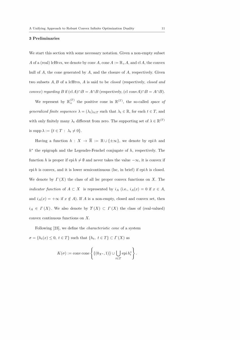
3 Preliminaries
We start this section with some necessary notation. Given a non-empty subset
A of a (real) lcHtvs, we denote by convA, coneA := R+A, and clA, the convex
hull of A, the cone generated by A, and the closure of A, respectively. Given
two subsets A,B of a lcHtvs, A is said to be closed (respectively, closed and
convex ) regarding B if (clA)∩B = A∩B (respectively, (cl convA)∩B = A∩B).
We represent by R(T )+ the positive cone in R(T ), the so-called space of
generalized finite sequences λ = (λt)t∈T such that λt ∈ R, for each t ∈ T, and
with only finitely many λt different from zero. The supporting set of λ ∈ R(T )
is suppλ := {t ∈ T : λt 6= 0}.
Having a function h : X → R := R ∪ {±∞}, we denote by epih and
h∗ the epigraph and the Legendre-Fenchel conjugate of h, respectively. The
function h is proper if epih 6= ∅ and never takes the value −∞, it is convex if
epih is convex, and it is lower semicontinuous (lsc, in brief) if epih is closed.
We denote by Γ (X) the class of all lsc proper convex functions on X. The
indicator function of A ⊂ X is represented by iA (i.e., iA(x) = 0 if x ∈ A,
and iA(x) = +∞ if x /∈ A). If A is a non-empty, closed and convex set, then
iA ∈ Γ (X) . We also denote by Υ (X) ⊂ Γ (X) the class of (real-valued)
convex continuous functions on X.
Following [23], we define the characteristic cone of a system
σ = {ht(x) ≤ 0, t ∈ T} such that {ht, t ∈ T} ⊂ Γ (X) as
K(σ) := conv cone
{{(0X∗ , 1)} ∪
⋃t∈T
epih∗t
}.
Page 12
12 Nguyen Dinh et al.
Concerning the data in the robust counterpart problem (RPx∗) introduced in
(2), we assume that, for each t ∈ T , Ut is an arbitrary subset of the lcHtvs Zt.
Along all the paper we will assume that
f ∈ Γ (X)
gt(·, ut) ∈ Υ (X) , ∀t ∈ T, ∀ut ∈ Ut,
∃x ∈ dom f : gt(x, ut) ≤ 0, ∀t ∈ T, ∀ut ∈ Ut.
(4)
If we denote by
U := {(t, ut) : t ∈ T, ut ∈ Ut}
the disjoint union of the sets Ut, t ∈ T , then the robust counterpart to the
uncertain problem (Px∗) can be rewritten as
(RPx∗) infx∈X{f(x)− 〈x∗, x〉 s.t. gt(x, ut) ≤ 0, ∀(t, ut) ∈ U} ,
whose feasible set F is represented by the (possibly) infinite convex system of
constraints σ := {gt(x, ut) ≤ 0, (t, ut) ∈ U}.
Throughout the paper we assume that F ∩ dom f 6= ∅, and so
inf(RPx∗) < +∞. Given u = (ut)t∈T ∈∏t∈T Ut = U , let us consider the
convex infinite problem
(Pux∗) infx∈X{f(x)− 〈x∗, x〉} s.t. gt(x, ut) ≤ 0, ∀t ∈ T,
whose feasible set Fu and constraint inequality system σu are independent of
x∗, and whose characteristic cone Ku := K (σu) can be expressed as
Ku = conv cone
{{(0X∗ , 1)} ∪
( ⋃t∈T
epi (gt(·, ut))∗)}
= R+{(0X∗ , 1)} ∪
⋃λ∈R(T )
+
∑t∈T
λt epi (gt(·, ut))∗ .
Page 13
A Unifying Approach to Robust Convex Infinite Optimization Duality 13
Since the functions gt(·, ut) are convex we have that, by Moreau-Rockafellar
formula and from the continuity assumption in (4) (entailing the w∗- closedness
of∑t∈T
epi (λtgt(·, ut))∗), we get
epi
(∑t∈T
λtgt(·, ut)
)∗=
∑t∈T
λt epi (gt(·, ut))∗ , if λ = (λt)t∈T 6= 0T ,
R+{(0X∗ , 1)}, else.
Hence,
Ku =⋃
λ∈R(T )+
epi
(∑t∈T
λtgt(·, ut)
)∗. (5)
By analogy (up to the sign) with [10], on uncertain linear semi-infinite case
(the terminology being a bit different in [7] for robust convex programming),
we have defined the robust moment cone (non-convex in general) by
MO :=⋃u∈U
Ku, (6)
and the robust characteristic cone as
MC := convMO.
Proposition 3.1 MC coincides with the characteristic cone K(σ) of the con-
vex system σ.
Page 14
14 Nguyen Dinh et al.
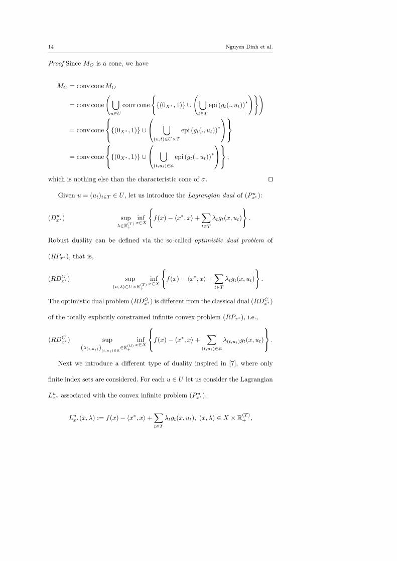
Proof Since MO is a cone, we have
MC = conv coneMO
= conv cone
(⋃u∈U
conv cone
{{(0X∗ , 1)} ∪
(⋃t∈T
epi (gt(., ut))∗
)})
= conv cone
{(0X∗ , 1)} ∪
⋃(u,t)∈U×T
epi (gt(., ut))∗
= conv cone
{(0X∗ , 1)} ∪
⋃(t,ut)∈U
epi (gt(., ut))∗
,
which is nothing else than the characteristic cone of σ. ut
Given u = (ut)t∈T ∈ U , let us introduce the Lagrangian dual of (Pux∗):
(Dux∗) sup
λ∈R(T )+
infx∈X
{f(x)− 〈x∗, x〉+
∑t∈T
λtgt(x, ut)
}.
Robust duality can be defined via the so-called optimistic dual problem of
(RPx∗), that is,
(RDOx∗) sup
(u,λ)∈U×R(T )+
infx∈X
{f(x)− 〈x∗, x〉+
∑t∈T
λtgt(x, ut)
}.
The optimistic dual problem (RDOx∗) is different from the classical dual (RDC
x∗)
of the totally explicitly constrained infinite convex problem (RPx∗), i.e.,
(RDCx∗) sup
(λ(t,ut))(t,ut)∈U∈R(U)
+
infx∈X
f(x)− 〈x∗, x〉+∑
(t,ut)∈U
λ(t,ut)gt(x, ut)
.
Next we introduce a different type of duality inspired in [7], where only
finite index sets are considered. For each u ∈ U let us consider the Lagrangian
Lux∗ associated with the convex infinite problem (Pux∗),
Lux∗(x, λ) := f(x)− 〈x∗, x〉+∑t∈T
λtgt(x, ut), (x, λ) ∈ X × R(T )+ ,
Page 15
A Unifying Approach to Robust Convex Infinite Optimization Duality 15
and define the robust Lagrangian L : X × R(T )+ → R by Lx∗ := supu∈U L
ux∗ .
One has
supλ∈R(T )
+
Lx∗(x, λ) = f(x)− 〈x∗, x〉+ iF (x), ∀x ∈ X,
and, consequently, (RPx∗) can be rewritten as
(RPx∗) infx∈X
supλ∈R(T )
+
Lx∗(x, λ).
The associated Lagrangian robust dual problem is defined by
(RDLhx∗ ) sup
λ∈R(T )+
infx∈X
supu∈U
{f(x)− 〈x∗, x〉+
∑t∈T
λtgt(x, ut)
}.
Let us give a clarifying interpretation of this Lagrangian robust dual. We start
by defining, for each t ∈ T, the function
ht := suput∈Ut
gt(·, ut),
which brings together the uncertain constraints gt(x, ut) ≤ 0, ut ∈ Ut, giving,
for each t ∈ T, the worse possible constraint. Observe that ht ∈ Γ (X), and it
is continuous (and belongs to Υ (X)) if Ut is a compact subset of Zt and the
function gt : X × Ut → R is continuous for all t ∈ T . Moreover
supu∈U
∑t∈T
λtgt(x, ut) =∑t∈T
λtht(x), ∀(x, λ) ∈ X × R(T )+ ,
and (RDLhx∗ ) can be written as
(RDLhx∗ ) sup
λ∈R(T )+
infx∈X
{f(x)− 〈x∗, x〉+
∑t∈T
λtht(x)
};
in other words (RDLhx∗ ) is the classical dual of the partially and explicitly
constrained infinite convex problem
(RPLhx∗ ) inf
x∈X{f(x)−〈x∗, x〉 s.t. ht(x) ≤ 0, ∀t ∈ T}.
Page 16
16 Nguyen Dinh et al.
In a similar way, for each u = (ut)t∈T ∈ U , we can define the function
ku := supt∈T
gt(·, ut),
which is a proper function thanks to (4), bringing together the constraints
gt(x, ut) ≤ 0, t ∈ T , for each u ∈ U . So, ku ∈ Γ (X), and it is continuous (and
belongs to Υ (X)) if T is a compact topological space and the function
(x, t) ∈ X × T 7→ gt(x, ut) is continuous, ∀u = (ut)t∈T ∈ U.
Then, the problem (RPx∗) can be rewritten as the partially and explicitly
constrained infinite convex problem
(RPLkx∗ ) inf
x∈X{f(x)−〈x∗, x〉 s.t. ku(x) ≤ 0, ∀u ∈ U},
and we consider its classical dual
(RDLkx∗ ) sup
λ∈R(U)+
infx∈X
{f(x)− 〈x∗, x〉+
∑u∈U
λuku(x)
}.
The problem (RDLkx∗ ) constitutes another kind of Lagrangian robust dual prob-
lem of (RPx∗). It is absolutely obvious that
inf(RPx∗) = inf(RPLhx∗ ) = inf(RPLk
x∗ ).
Let us explore next the relationship among the optimal values of the different
duals introduced above.
Proposition 3.2 For every x∗ ∈ X∗ and i ∈ {Lh, Lk} , one has
sup(RDOx∗) ≤
supu∈U
inf(Pux∗)
sup(RDCx∗) ≤ sup(RDi
x∗)
≤ inf(RPx∗). (7)
Page 17
A Unifying Approach to Robust Convex Infinite Optimization Duality 17
Proof • For each (u, λ) ∈ U × R(T )+ one has
∑t∈T λtgt(·, ut) ≤ iFu
and
infX
{f − 〈x∗, ·〉+
∑t∈T
λtgt(·, ut)
}≤ inf
Fu
(f − 〈x∗, ·〉) = inf(Pux∗).
Taking the supremum over (u, λ) ∈ U×R(T )+ we get sup(RDO
x∗)≤ supu∈U
inf(Pux∗).
• If (u, λ) ∈ U × R(T )+ , let us define
λ(t,ut) :=
λt, if ut = ut,
0, if ut 6= ut.
We have (λ(t,ut))(t,ut)∈U ∈ R(U)+ , and
∑t∈T
λtgt(·, ut) =∑
(t,ut)∈Uλ(t,ut)gt(·, ut). It
easily follows that sup(RDOx∗) ≤ sup(RDC
x∗).
• Besides, since for each u ∈ U , the feasible set Fu of (Pux∗) contains the feasible
set F of (RPx∗), we have supu∈U
inf(Pux∗) ≤ inf(RPx∗).
• We now prove that sup(RDCx∗) ≤ sup(RDLh
x∗ ). If λ ∈ R(U)+ then we will show
that
infx∈X
f(x)− 〈x∗, x〉+∑
(t,ut)∈U
λ(t,ut)gt(x, ut)
≤ sup(RDLhx∗ ).
For each t ∈ T , define λt :=∑
(t,ut)∈suppλλ(t,ut). Then, λ := (λt)t∈T belongs to
R(T )+ and we have, for each x ∈ X,
∑(t,ut)∈U
λ(t,ut)gt(x, ut) ≤∑
(t,ut)∈U
λ(t,ut)ht(x) =∑t∈T
λtht(x).
It follows that
infx∈X
f(x)− 〈x∗, x〉+∑
(t,ut)∈U
λ(t,ut)gt(x, ut)
≤ infx∈X
{f(x)− 〈x∗, x〉+
∑t∈T
λtht(x)
}≤ sup(RDLh
x∗ ).
Page 18
18 Nguyen Dinh et al.
• We also have that sup(RDCx∗) ≤ sup(RDLk
x∗ ). If λ ∈ R(U)+ then we will see
that
infx∈X
f(x)− 〈x∗, x〉+∑
(t,ut)∈U
λ(t,ut)gt(x, ut)
≤ sup(RDLkx∗ ).
For each u = (ut)t∈T ∈ U , define λu :=∑
(t,ut)∈suppλλ(t,ut). Then, λ := (λu)u∈U
belongs to R(U)+ and we have, for each x ∈ X,
∑(t,ut)∈U
λ(t,ut)gt(x, ut) ≤∑
(t,ut)∈U
λ(t,ut)ku(x) =∑u∈U
λuku(x).
It follows that
infx∈X
f(x)− 〈x∗, x〉+∑
(t,ut)∈U
λ(t,ut)gt(x, ut)
≤ infx∈X
{f(x)− 〈x∗, x〉+
∑u∈U
λuku(x)
}≤ sup(RDLk
x∗ ).
• It is easy to see that sup(LRDix∗) ≤ inf(RPx∗), i ∈ {Lh, Lk} , and the proof
is complete. ut
We illustrate next the case when T is a singleton, U is a compact topological
space and g : X × U → R is such that g(., u) is continuous and convex for
each u ∈ U and g(x, .) is upper semicontinuous for each x ∈ X. We thus have
(RDOx∗) sup
λ≥0supu∈U
[infx∈X{f(x)− 〈x∗, x〉+ λg(x, u)}
],
(RDCx∗) = (RDLk
x∗ ) supλ∈R(U)
+
[infx∈X
{f(x)− 〈x∗, x〉+
∑u∈U
λug(x, u)
}],
(RDLhx∗ ) sup
λ≥0
[infx∈X{f(x)− 〈x∗, x〉+ λh(x)}
],
where h(x) = maxu∈U g(x, u).
Page 19
A Unifying Approach to Robust Convex Infinite Optimization Duality 19
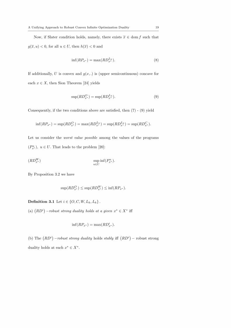
Now, if Slater condition holds, namely, there exists x ∈ dom f such that
g(x, u) < 0, for all u ∈ U, then h(x) < 0 and
inf(RPx∗) = max(RDLhx∗ ). (8)
If additionally, U is convex and g(x, .) is (upper semicontinuous) concave for
each x ∈ X, then Sion Theorem [24] yields
sup(RDOx∗) = sup(RDLh
x∗ ). (9)
Consequently, if the two conditions above are satisfied, then (7) - (9) yield
inf(RPx∗) = sup(RDOx∗) = max(RDLh
x∗ ) = sup(RDLkx∗ ) = sup(RDC
x∗).
Let us consider the worst value possible among the values of the programs
(Pux∗), u ∈ U . That leads to the problem [20]:
(RDWx∗) sup
u∈Uinf(Pux∗).
By Proposition 3.2 we have
sup(RDOx∗) ≤ sup(RDW
x∗) ≤ inf(RPx∗).
Definition 3.1 Let i ∈ {O,C,W,Lh, Lk} .
(a)(RDi
)−robust strong duality holds at a given x∗ ∈ X∗ iff
inf(RPx∗) = max(RDix∗).
(b) The(RDi
)−robust strong duality holds stably iff
(RDi
)− robust strong
duality holds at each x∗ ∈ X∗.
Page 20
20 Nguyen Dinh et al.
(c) The(RDi
)−robust strong duality holds uniformly iff
(RDi
)−robust strong
duality holds at x∗ = 0X∗ for any function f in the family
F := {f ∈ Γ (X) : f is continuous at some point of F} .
(Observe that f ∈F entails f − 〈x∗, .〉 ∈F , ∀x∗ ∈ X∗).
From the proof of Proposition 3.2 it is clearly that optimistic robust strong
duality entails classical robust strong duality, Lagrangian robust strong duality
of both types and worst-value robust strong duality. Robust strong duality of
the types defined in (a) and (b) in Definition 3.1 will be studied in next section
(Section 4), while the last one and some more complements will be given in
Section 5.
We conclude this section by the following note: For the sake of simplicity,
in the case when x∗ = 0X∗ the robust dual problems (RDi0X∗
) will be denoted,
respectively, by (RDi), i ∈ {O,C,W,Lh, Lk}.
4 The Main Results
In this section, we will study common duality principles between (RPx∗)
and the dual problems (RDi), i ∈ {O,C,W,Lh, Lk}. For this, let us as-
sociate the mentioned dual problems with the functions ϕi : X∗ −→ R,
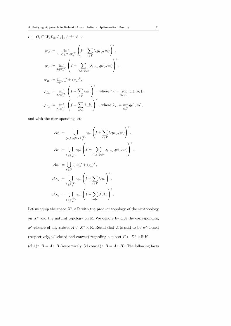
Page 21
A Unifying Approach to Robust Convex Infinite Optimization Duality 21
i ∈ {O,C,W,Lh, Lk} , defined as
ϕO := inf(u,λ)∈U×R(T )
+
(f +
∑t∈T
λtgt(., ut)
)∗,
ϕC := infλ∈R(U)
+
f +∑
(t,ut)∈U
λ(t,ut)gt(., ut)
∗ ,ϕW := inf
u∈U(f + iFu
)∗,
ϕLh:= inf
λ∈R(T )+
(f +
∑t∈T
λtht
)∗, where ht := sup
ut∈Ut
gt(., ut),
ϕLk:= inf
λ∈R(U)+
(f +
∑u∈U
λuku
)∗, where ku := sup
t∈Tgt(., ut),
and with the corresponding sets
AO :=⋃
(u,λ)∈U×R(T )+
epi
(f +
∑t∈T
λtgt(., ut)
)∗,
AC :=⋃
λ∈R(U)+
epi
f +∑
(t,ut)∈U
λ(t,ut)gt(., ut)
∗ ,AW :=
⋃u∈U
epi (f + iFu)∗,
ALh:=
⋃λ∈R(T )
+
epi
(f +
∑t∈T
λtht
)∗,
ALk:=
⋃λ∈R(U)
+
epi
(f +
∑u∈U
λuku
)∗.
Let us equip the space X∗ ×R with the product topology of the w∗-topology
on X∗ and the natural topology on R. We denote by clA the corresponding
w∗-closure of any subset A ⊂ X∗ × R. Recall that A is said to be w∗-closed
(respectively, w∗-closed and convex) regarding a subset B ⊂ X∗ × R if
(clA)∩B = A∩B (respectively, (cl convA)∩B = A∩B). The following facts
Page 22
22 Nguyen Dinh et al.
can easily be checked (the convexity of the sets and functions below can be
proved by a similar reasoning to the one followed in Lemma 3.1 in [25]):
Ai ⊂ epiϕi ⊂ cl(Ai), i ∈ {O,C,W,Lh, Lk} ,
AC ,ALh, and ALk
are convex sets,
ϕC , ϕLh, and ϕLk
are convex functions.
(10)
Let us give some equivalent expressions of the sets Ai, i ∈ {O,C,W,Lh, Lk} ,
respectively in terms of the robust moment cones with the same indexes and
the characteristic cones Ku, u ∈ U .
Proposition 4.1 (a) One has
AO = epi f∗ +MO, AC = epi f∗ +MC , AW =⋃u∈U
cl (epi f∗ +Ku) .
(b) If f ∈ F , then AW = epi f∗ +⋃u∈U cl (Ku) = epi f∗ +MW .
(c) If ht ∈ Υ (X) , ∀t ∈ T, then ALh= epi f∗ +MLh
.
(d) If ku ∈ Υ (X) , ∀ u ∈ U, then ALk= epi f∗ +MLk
.
Proof (a) By Moreau-Rockafellar formula (as∑t∈T λtgt(·, ut) are continuous),
AO =⋃
(u,λ)∈U×R(T )+
(epi f∗ + epi
(∑t∈T
λtgt(·, ut)
)∗)
= epi f∗ +⋃
(u,λ)∈U×R(T )+
epi
(∑t∈T
λtgt(·, ut)
)∗
= epi f∗ +⋃u∈U
Ku = epi f∗ +MO.
Page 23
A Unifying Approach to Robust Convex Infinite Optimization Duality 23
AC :=⋃
λ∈R(U)+
epi f∗ + epi
∑(t,ut)∈U
λ(t,ut)gt(·, ut)
∗= epi f∗ +
⋃λ∈R(U)
+
epi
∑(t,ut)∈U
λ(t,ut)gt(·, ut)
∗ = epi f∗ +MC .
In order to have an explicit expression of AW , let us observe that for all
u = (ut)t∈T ∈ U, iFu= sup
λ∈R(T )+
∑t∈T λtgt(·, ut). Since Fu 6= ∅,
epi i∗Fu= cl conv
⋃λ∈R(T )
+
epi∑t∈T
λtgt(., ut)∗
= cl conv(Ku) = cl(Ku)
(as Ku is convex), and then
AW =⋃u∈U
cl(epi f∗ + epi i∗Fu
)=⋃u∈U
cl (epi f∗ + cl(Ku))=⋃u∈U
cl (epi f∗ +Ku) .
(b) Since f ∈ F , we have
epi(f + iFu)∗ = epi f∗ + epi i∗Fu= epi f∗ + cl(Ku), ∀u ∈ U.
We now observe that
cl(Ku) = cl conv cone
(⋃t∈T
epi(gt(., ut))∗
), ∀u ∈ U. (11)
By the very definition of Ku, the inclusion ⊃ in (11) is obvious. Conversely,
let us first check that (0X∗ , 1) ∈ cl cone (epi(gt(., ut))∗) for any t ∈ T . Pick
(x∗, r) ∈ epi(gt(., ut))∗. For each n ≥ 1 we have 1
n (x∗, r+n) ∈ cone epi(gt(., ut))∗,
and (0X∗ , 1) = limn→∞
1n (x∗, r + n) ∈ cl cone (epi(gt(., ut))
∗). Now it is clearly
that (0X∗ , 1) belongs to the right-hand side of (11). By definition of Ku it
Page 24
24 Nguyen Dinh et al.
follows that Ku is contained in the right-hand side of (11), which is closed.
Finally, we get that (11) holds. We thus have
AW =⋃u∈U
(epi f∗ + clKu) = epi f∗ +⋃u∈U
clKu
= epi f∗ +⋃u∈U
{cl conv cone
(⋃t∈T
epi(gt(., ut))∗
)}= epi f∗ +MW .
(c) For each λ ∈ R(T )+ one has
∑t∈T
λtht ∈ Υ (X) and, by this,
epi
(f +
∑t∈T
λtht
)∗= epi f∗ + epi
(∑t∈T
λtht
)∗.
We thus have,
ALh= epi f∗ +
⋃λ∈R(T )
+
epi
(∑t∈T
λtht
)∗.
Since ht ∈ Υ (X) for all t ∈ T , one has, for each λ ∈ R(T )+ :
epi
(∑t∈T
λtht
)∗=
∑t∈T
λt epih∗t , if λ = (λt)t∈T 6= 0T ,
{0X∗} × R+, else.
Therefore,
⋃λ∈R(T )
+
epi
(∑t∈T
λtht
)∗
= R+{(0X∗ , 1)} ∪
⋃λ∈R(T )
+
∑t∈T
λt epih∗t
= conv cone
{{(0X∗ , 1)} ∪
(⋃t∈T
epih∗t
)}
= conv cone
{{(0X∗ , 1)} ∪
(⋃t∈T
cl conv⋃
ut∈Ut
epi(gt(., ut))∗
)},
and the proof of (c) is complete.
(d) The proof is similar to that of (c). ut
Page 25
A Unifying Approach to Robust Convex Infinite Optimization Duality 25
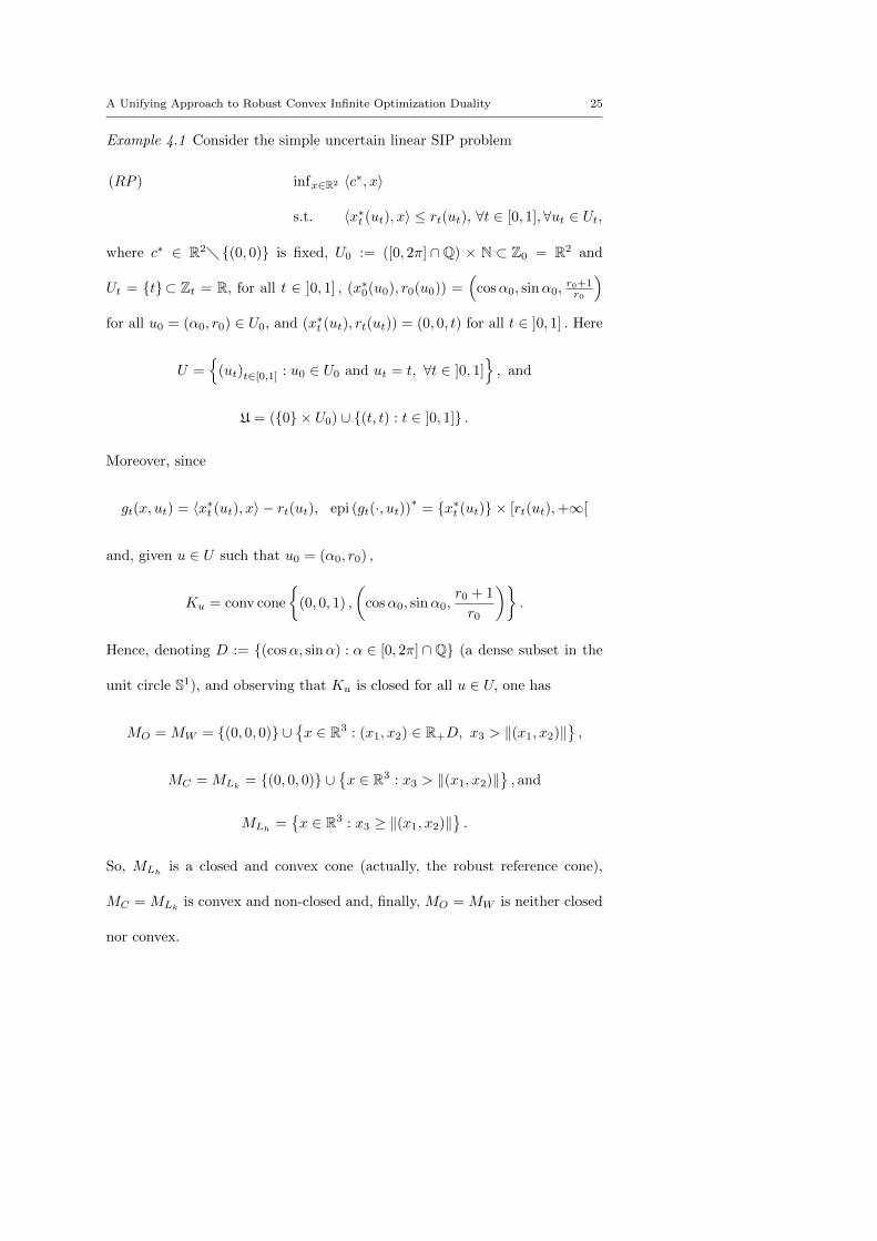
Example 4.1 Consider the simple uncertain linear SIP problem
(RP ) infx∈R2 〈c∗, x〉
s.t. 〈x∗t (ut), x〉 ≤ rt(ut), ∀t ∈ [0, 1],∀ut ∈ Ut,
where c∗ ∈ R2� {(0, 0)} is fixed, U0 := ([0, 2π] ∩Q) × N ⊂ Z0 = R2 and
Ut = {t}⊂ Zt = R, for all t ∈ ]0, 1] , (x∗0(u0), r0(u0)) =(
cosα0, sinα0,r0+1r0
)for all u0 = (α0, r0) ∈ U0, and (x∗t (ut), rt(ut)) = (0, 0, t) for all t ∈ ]0, 1] . Here
U ={
(ut)t∈[0,1] : u0 ∈ U0 and ut = t, ∀t ∈ ]0, 1]}, and
U = ({0} × U0) ∪ {(t, t) : t ∈ ]0, 1]} .
Moreover, since
gt(x, ut) = 〈x∗t (ut), x〉 − rt(ut), epi (gt(·, ut))∗ = {x∗t (ut)} × [rt(ut),+∞[
and, given u ∈ U such that u0 = (α0, r0) ,
Ku = conv cone
{(0, 0, 1) ,
(cosα0, sinα0,
r0 + 1
r0
)}.
Hence, denoting D := {(cosα, sinα) : α ∈ [0, 2π] ∩Q} (a dense subset in the
unit circle S1), and observing that Ku is closed for all u ∈ U, one has
MO = MW = {(0, 0, 0)} ∪{x ∈ R3 : (x1, x2) ∈ R+D, x3 > ‖(x1, x2)‖
},
MC = MLk= {(0, 0, 0)} ∪
{x ∈ R3 : x3 > ‖(x1, x2)‖
}, and
MLh={x ∈ R3 : x3 ≥ ‖(x1, x2)‖
}.
So, MLhis a closed and convex cone (actually, the robust reference cone),
MC = MLkis convex and non-closed and, finally, MO = MW is neither closed
nor convex.
Page 26
26 Nguyen Dinh et al.
The functions ht are continuous for all t ∈ [0, 1] as, given x ∈ R2, ht (x) = −t
if t > 0, while
h0 (x) = sup{
(cosα0)x1 + (sinα0)x2 − r0+1r0
: α0 ∈ [0, 2π] ∩Q, r0 ∈ N}
= sup {(cosα0)x1 + (sinα0)x2 − 1 : α0 ∈ [0, 2π]} = ‖x‖ − 1.
Similarly, the functions ku are continuous for all u = (ut)t∈[0,1] ∈ U as, given
x ∈ R2,
ku (x) = supt∈T (〈x∗t (ut), x〉 − rt(ut))
= max{
(cosα0)x1 + (sinα0)x2 − r0+1r0
, 0}
is the maximum of two affine functions. It is obvious that
F = {x ∈ R2 : ‖x‖ ≤ 1}, inf(RP ) = −‖c∗‖, and epi (〈c∗, x〉)∗ = {c∗} × R+.
We conclude that Ai = Mi + (c∗1, c∗2, 0) , i ∈ {O,C,W,Lh, Lk} , which have
the same topological and convexity properties as the corresponding moment
cones.
Now we proceed by introducing the function p := f + iF . It holds that
infx∈X{p− 〈x∗, ·〉} = inf(RPx∗) and p ∈ Γ (X) (entailing p = p∗∗).
The two propositions below are mere consequences of Proposition 3.2, as
p∗(x∗) = − inf(RPx∗),
ϕi(x∗) = − sup(RDi
x∗), ∀i ∈ {O,C,W,Lh, Lk} .
Proposition 4.2 For every x∗ ∈ X∗ and i ∈ {Lh, Lk} one has
p∗(x∗) ≤ϕW (x∗)
ϕi(x∗) ≤ ϕC(x∗)
≤ ϕO(x∗).
Page 27
A Unifying Approach to Robust Convex Infinite Optimization Duality 27
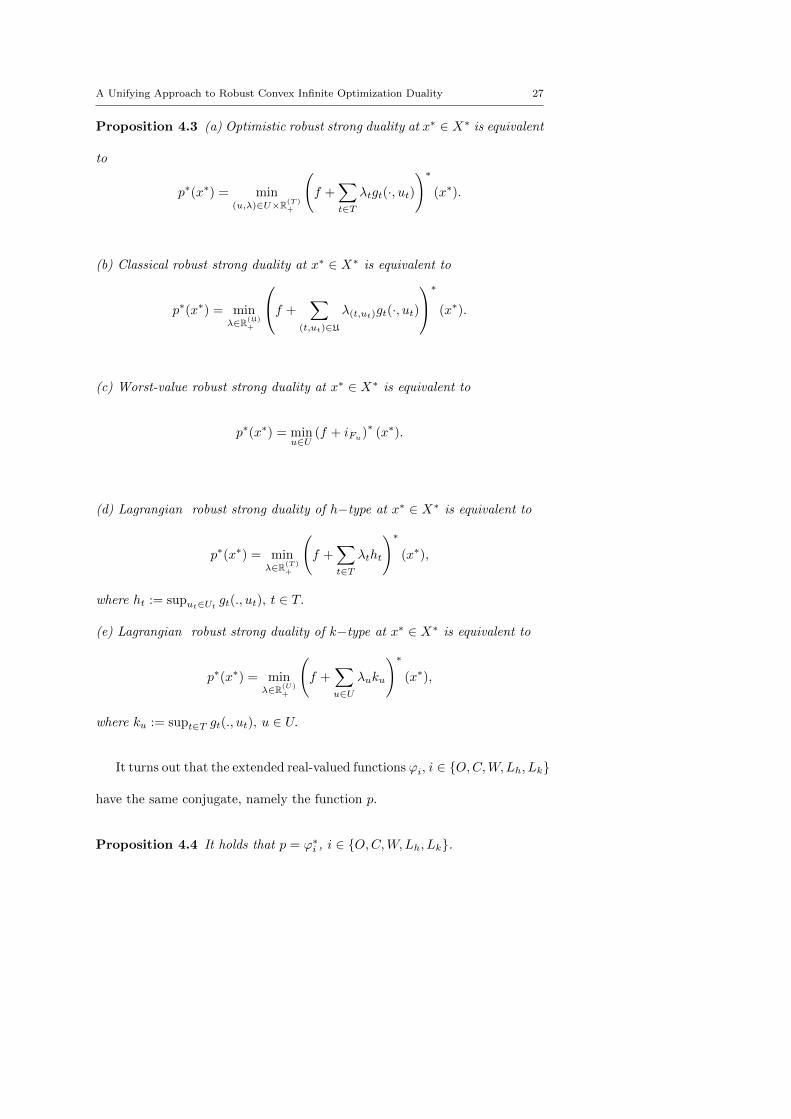
Proposition 4.3 (a) Optimistic robust strong duality at x∗ ∈ X∗ is equivalent
to
p∗(x∗) = min(u,λ)∈U×R(T )
+
(f +
∑t∈T
λtgt(·, ut)
)∗(x∗).
(b) Classical robust strong duality at x∗ ∈ X∗ is equivalent to
p∗(x∗) = minλ∈R(U)
+
f +∑
(t,ut)∈U
λ(t,ut)gt(·, ut)
∗ (x∗).
(c) Worst-value robust strong duality at x∗ ∈ X∗ is equivalent to
p∗(x∗) = minu∈U
(f + iFu)∗
(x∗).
(d) Lagrangian robust strong duality of h−type at x∗ ∈ X∗ is equivalent to
p∗(x∗) = minλ∈R(T )
+
(f +
∑t∈T
λtht
)∗(x∗),
where ht := suput∈Utgt(., ut), t ∈ T.
(e) Lagrangian robust strong duality of k−type at x∗ ∈ X∗ is equivalent to
p∗(x∗) = minλ∈R(U)
+
(f +
∑u∈U
λuku
)∗(x∗),
where ku := supt∈T gt(., ut), u ∈ U.
It turns out that the extended real-valued functions ϕi, i ∈ {O,C,W,Lh, Lk}
have the same conjugate, namely the function p.
Proposition 4.4 It holds that p = ϕ∗i , i ∈ {O,C,W,Lh, Lk}.
Page 28
28 Nguyen Dinh et al.
Proof By Proposition 4.2 it suffices to check that p = ϕ∗O. Now
ϕ∗O =
(inf
(u,λ)∈U×R(T )+
(f +∑t∈T
λtgt(., ut)
)∗)∗= sup
(u,λ)∈U×R(T )+
(f +
∑t∈T
λtgt(., ut)
)∗∗
= sup(u,λ)∈U×R(T )
+
(f +
∑t∈T
λtgt(., ut)
)= f + sup
(u,λ)∈U×R(T )+
(∑t∈T
λtgt(., ut)
)
= f + supu∈U
supλ∈R(T )
+
(∑t∈T
λtgt(., ut)
)= f + sup
u∈UiFu
= f + iF = p. ut
Proposition 4.5 One has
epi p∗ = cl conv(epi f∗ +MO) = cl (epi f∗ +MC)
= cl conv
(⋃u∈U
cl (epi f∗ +Ku)
)= cl conv
(epi f∗ +
⋃u∈U
Ku
),
or, equivalently,
epi p∗ = cl conv(AO) = cl(AC) = cl conv(AW ).
If ht ∈ Υ (X) for all t ∈ T (resp. ku ∈ Υ (X) for all u ∈ U), then we have
additionally
epi p∗ = cl(ALh) (respectively, epi p∗ = cl(ALk
)).
Proof By (10) we have cl conv(Ai) = cl conv(epiϕi), i ∈ {O,W} , and
cl(Ai) = cl (epi ϕi), i ∈ {C,Lh, Lk} . Since dom p 6= ∅, Proposition 4.4 and
Proposition 4.1 give
epi p∗ = epiϕ∗∗i = cl conv(epiϕi) = cl conv(Ai), i ∈ {O,W} .
epi p∗ = epiϕ∗∗C = cl (epi ϕC) = cl(AC).
Page 29
A Unifying Approach to Robust Convex Infinite Optimization Duality 29
The rest of equations in the first statement follow from Proposition 4.1.
If ht ∈ Υ (X) for all t ∈ T, then
epi p∗ = epiϕ∗∗Lh= cl (epi ϕLh
) = cl(ALh).
The last statement, involving ALk, holds similarly. ut
We are now in a position to establish the duality principles corresponding
to the dual problems (RDix∗), i ∈ {O,C,W,Lh, Lk}. In the special cases, these
duality principles lead to characterizations of robust and robust stable strong
duality between (RP ) and (RDix∗), i ∈ {O,C,W,Lh, Lk}. The theorems below
extend, complete and unify some results in the literature; in particular, some
results concerning optimistic robust duality in [4, 6–10, 13–15, 19, 20, 26], etc.,
classical robust duality in [10], Lagrangian robust duality of type Lh in [7],
etc.
Theorem 4.1 (Robust strong duality at a point) Let i ∈ {O,C,W,Lh, Lk}
be such that ht ∈ Υ (X) for all t ∈ T when i = Lh, and that ku ∈ Υ (X) for
all u ∈ U when i = Lk. Then, given x∗ ∈ X∗,(RDi
)−robust strong duality
holds at x∗ if and only if Ai is w∗-closed and convex regarding {x∗} × R for
i ∈ {O,W}, and w∗-closed regarding {x∗} × R for i ∈ {C,Lh, Lk}.
Proof We discuss the five possible cases.
• Case i = O: By Proposition 4.5 we have
({x∗}×R)∩ cl conv(AO) = ({x∗}×R)∩ epi p∗ = {x∗}×{r ∈ R : p∗(x∗) ≤ r}.
(12)
Page 30
30 Nguyen Dinh et al.
Let us begin with the case that p∗(x∗) = +∞. By (12) we have
({x∗}×R)∩cl conv(AO) = ∅ and, hence, AO is w∗-closed and convex regarding
{x∗} × R. By Proposition 4.2 we have ϕO(x∗) = +∞, and
infx∈F{f(x)− 〈x∗, x〉} = −p∗(x∗) = −∞ = −ϕO(x∗) =
= max(u,λ)∈U×R(T )
+
infx∈X
{f(x)− 〈x∗, x〉+
∑t∈T
λtgt(x, ut)
},
the maximum being attained at each (u, λ) ∈ U × R(T )+ . So, if p∗(x∗) = +∞,
then both statements in Theorem 4.1 are true.
Consider now that p∗(x∗) 6= +∞. Since dom p 6= ∅, we get p∗(x∗) ∈ R. By
Proposition 4.5 we have (x∗, p∗(x∗)) ∈ cl conv(AO).
Assume first thatAO is w∗-closed and convex regarding {x∗}×R. We then have
(x∗, p∗(x∗)) ∈ AO, and by the definition of AO, there exists (u, λ) ∈ U ×R(T )+
such that
(x∗, p∗(x∗)) ∈ epi
(f +
∑t∈T
λtgt(., ut)
)∗. (13)
Now, combining the definition of ϕO with (13) and Proposition 4.2, one gets
ϕO(x∗) ≤
(f +
∑t∈T
λtgt(., ut)
)∗(x∗) ≤ p∗(x∗) ≤ ϕO(x∗).
It follows that
p∗(x∗) =
(f +
∑t∈T
λtgt(., ut)
)∗(x∗) = min
(u,λ)∈U×R(T )+
(f +
∑t∈T
λtgt(., ut)
)∗(x∗),
and, taking Proposition 4.3(a) into account, optimistic robust strong duality
holds at x∗.
Conversely, assume that optimistic robust strong duality holds at x∗, and let
(x∗, r) ∈ cl conv(AO) = epi p∗. One has to check that (x∗, r) ∈ AO. As the
Page 31
A Unifying Approach to Robust Convex Infinite Optimization Duality 31
optimistic robust strong duality holds at x∗, there exists (u, λ) ∈ U × R(T )+
such that(f +
∑t∈T λtgt(., ut)
)∗(x∗) = p∗(x∗) ≤ r (see Proposition 4.3(a)),
showing that (x∗, r) ∈ epi(f +
∑t∈T λtgt(., ut)
)∗ ⊂ AO.
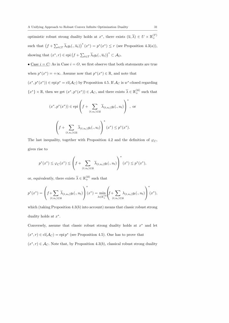
• Case i = C: As in Case i = O, we first observe that both statements are true
when p∗(x∗) = +∞. Assume now that p∗(x∗) ∈ R, and note that
(x∗, p∗(x∗)) ∈ epi p∗ = cl(AC) by Proposition 4.5. If AC is w∗-closed regarding
{x∗} × R, then we get (x∗, p∗(x∗)) ∈ AC , and there exists λ ∈ R(U)+ such that
(x∗, p∗(x∗)) ∈ epi
f +∑
(t,ut)∈U
λ(t,ut)gt(., ut)
∗ , or
f +∑
(t,ut)∈U
λ(t,ut)gt(., ut)
∗ (x∗) ≤ p∗(x∗).
The last inequality, together with Proposition 4.2 and the definition of ϕC ,
gives rise to
p∗(x∗) ≤ ϕC(x∗) ≤
f +∑
(t,ut)∈U
λ(t,ut)gt(., ut)
∗ (x∗) ≤ p∗(x∗),
or, equivalently, there exists λ ∈ R(U)+ such that
p∗(x∗) =
f+∑
(t,ut)∈U
λ(t,ut)gt(., ut)
∗(x∗) = minλ∈R(U)
+
f+∑
(t,ut)∈U
λ(t,ut)gt(., ut)
∗(x∗),which (taking Proposition 4.3(b) into account) means that classic robust strong
duality holds at x∗.
Conversely, assume that classic robust strong duality holds at x∗ and let
(x∗, r) ∈ cl(AC) = epi p∗ (see Proposition 4.5). One has to prove that
(x∗, r) ∈ AC . Note that, by Proposition 4.3(b), classical robust strong duality
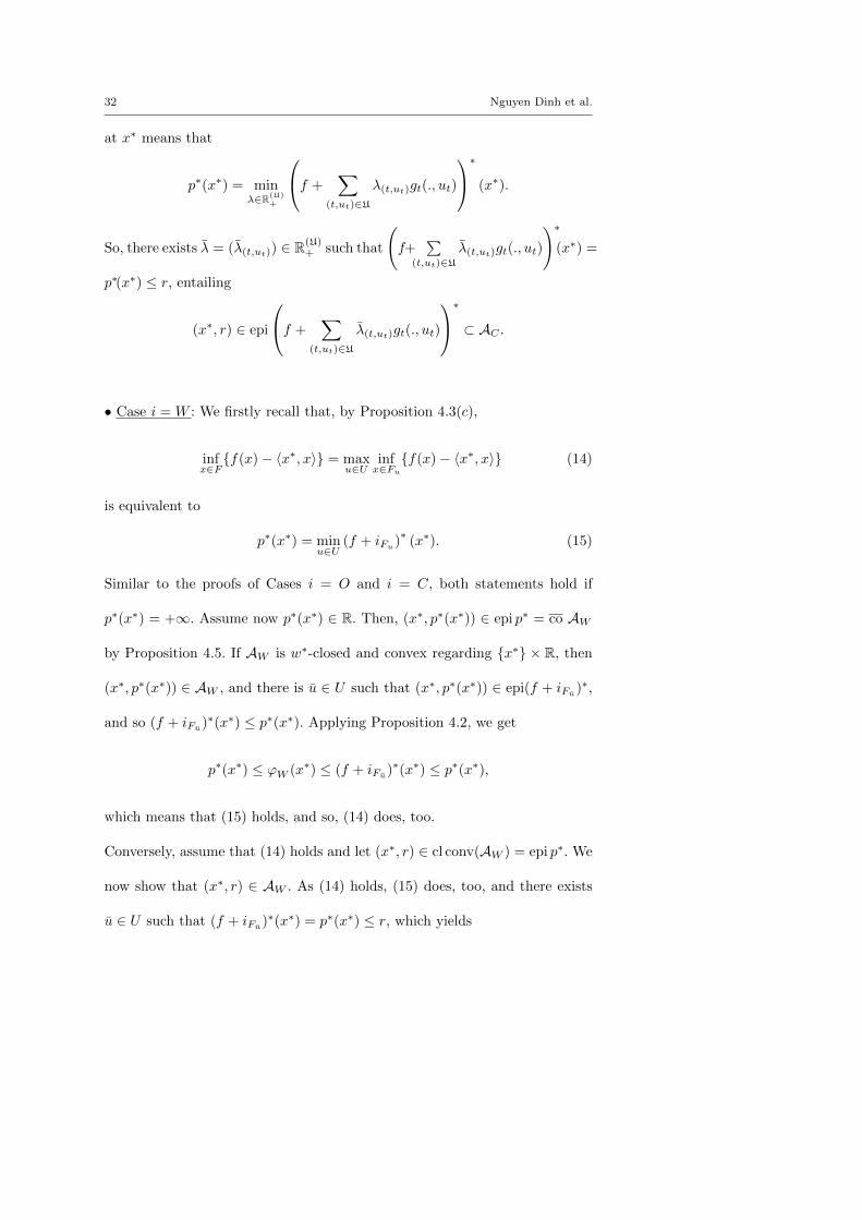
Page 32
32 Nguyen Dinh et al.
at x∗ means that
p∗(x∗) = minλ∈R(U)
+
f +∑
(t,ut)∈U
λ(t,ut)gt(., ut)
∗ (x∗).
So, there exists λ = (λ(t,ut)) ∈ R(U)+ such that
(f+
∑(t,ut)∈U
λ(t,ut)gt(., ut)
)∗(x∗) =
p∗(x∗) ≤ r, entailing
(x∗, r) ∈ epi
f +∑
(t,ut)∈U
λ(t,ut)gt(., ut)
∗ ⊂ AC .
• Case i = W : We firstly recall that, by Proposition 4.3(c),
infx∈F{f(x)− 〈x∗, x〉} = max
u∈Uinfx∈Fu
{f(x)− 〈x∗, x〉} (14)
is equivalent to
p∗(x∗) = minu∈U
(f + iFu)∗
(x∗). (15)
Similar to the proofs of Cases i = O and i = C, both statements hold if
p∗(x∗) = +∞. Assume now p∗(x∗) ∈ R. Then, (x∗, p∗(x∗)) ∈ epi p∗ = co AW
by Proposition 4.5. If AW is w∗-closed and convex regarding {x∗} × R, then
(x∗, p∗(x∗)) ∈ AW , and there is u ∈ U such that (x∗, p∗(x∗)) ∈ epi(f + iFu)∗,
and so (f + iFu)∗(x∗) ≤ p∗(x∗). Applying Proposition 4.2, we get
p∗(x∗) ≤ ϕW (x∗) ≤ (f + iFu)∗(x∗) ≤ p∗(x∗),
which means that (15) holds, and so, (14) does, too.
Conversely, assume that (14) holds and let (x∗, r) ∈ cl conv(AW ) = epi p∗. We
now show that (x∗, r) ∈ AW . As (14) holds, (15) does, too, and there exists
u ∈ U such that (f + iFu)∗(x∗) = p∗(x∗) ≤ r, which yields
Page 33
A Unifying Approach to Robust Convex Infinite Optimization Duality 33
(x∗, r) ∈ epi(f + iFu)∗ ⊂ AW .
• The proofs for cases i = Lh, assuming ht ∈ Υ (X) for all t ∈ T , and i = Lk,
assuming ku ∈ Υ (X) for all u ∈ U , are completely similar to the proof for
the case i = C (they also can be derived from [27, Theorem 1] with f being
replaced by f − x∗). ut
Next very important results are consequences of Theorem 4.1.
Theorem 4.2 (Robust strong duality) Let i ∈ {O,C,W,Lh, Lk} be such
that ht ∈ Υ (X) for all t ∈ T when i = Lh, and that ku ∈ Υ (X) for all u ∈ U
when i = Lk. Then,(RDi
)− robust strong duality holds for the robust coun-
terpart (RP ), i.e., inf (RP ) = max (RDi), if and only if Ai is w∗-closed and
convex regarding {0x∗}×R for i ∈ {O,W}, and w∗-closed regarding {0x∗}×R
for i ∈ {C,Lh, Lk}.
Theorem 4.3 (Stable strong duality) Let i ∈ {O,C,W,Lh, Lk} be such
that ht ∈ Υ (X) for all t ∈ T when i = Lh, and that ku ∈ Υ (X) for all u ∈ U
when i = Lk. Then,(RDi
)− robust strong duality holds stably if and only if
Ai is w∗-closed and convex for i ∈ {O,W}, and w∗-closed for i ∈ {C,Lh, Lk}.
In Example 4.1, Ai is closed and convex regarding {(0, 0)}×R if and only
if Mi is closed and convex regarding {−c∗} × R, which is true for i = Lh and
false for i ∈ {C,W,Lk}, as well as for i = O when Ai ∩ ({(0, 0)} × R) 6= ∅.
Thus, only (RDLh) is solvable, independently of the objective function. Since
ALhis w∗-closed and convex, (RDLh) enjoys stable robust strong duality.
Concerning optimistic robust strong duality (see Theorem 4.1, Case
i = O and the corresponding corollaries) the following question is of particular
Page 34
34 Nguyen Dinh et al.
interest: when is MO (hence, AO = epi f∗+MO) convex? Next result provides
an answer for that, including the ”convexity condition” introduced in [10]
for robust linear semi-infinite problems, and extending [7, Proposition 2.3] to
robust infinite convex programs.
Proposition 4.6 Assume that, for each t ∈ T , Ut is a convex subset of Zt
and that, for each x ∈ X, the function ut ∈ Ut 7→ gt(x, ut) is concave. Then,
the robust moment cone MO is convex.
Proof Let (x∗1, r1), (x∗2, r2) ∈ MO. Since MO is a cone, it suffices to check
that (x∗1 + x∗2, r1 + r2) ∈ MO. Taking into account (5) and (6), there exist
(u1, λ1), (u2, λ2) ∈ U × R(T )+ such that
〈x∗1, x〉 −∑t∈T
λ1t gt(x, u1t ) ≤ r1, ∀x ∈ X,
〈x∗2, x〉 −∑t∈T
λ2t gt(x, u2t ) ≤ r2, ∀x ∈ X.
Define λ0 := λ1 + λ2 ∈ R(T )+ , and u0 ∈
∏t∈T Zt such that
u0t :=
u1t , if λ0t = 0 (i.e., λ1t = λ2t = 0),
λ1t
λ0tu1t +
λ2t
λ0tu2t , else (i.e., if λ0t > 0).
Since, for each t ∈ T , Ut is convex, we have u0 ∈∏t∈T Ut = U . Let us check
that (x∗1 + x∗2, r1 + r2) ∈ epi(∑
t∈T λ0t gt(., u
0t ))∗
, and this will conclude the
proof. For each x ∈ X we have, since gt(x, .) is concave,
∑t∈T
λ0t gt(x, u0t ) ≥
∑t∈T
(λ1t gt(x, u
1t ) + λ2t gt(x, u
2t )),
Page 35
A Unifying Approach to Robust Convex Infinite Optimization Duality 35
and for any x ∈ X,
〈x∗1 + x∗2, x〉−∑t∈T
λ0t gt(x, u0t )≤ 〈x∗1, x〉−
∑t∈T
λ1t gt(x, u1t )+〈x∗2, x〉−
∑t∈T
λ2t gt(x, u2t )
≤ r1 + r2. ut
The last result in this section provides a sufficient condition for MW to be
convex. Recall that, since epi i∗Fu= cl(Ku), for all u ∈ U, MW =
⋃u∈U
epi i∗Fu,
where Fu = {x ∈ X : gt(x, ut) ≤ 0, t ∈ T} . Recall also that U is the disjoint
union of the sets Ut, t ∈ T , and that U =∏t∈T Ut.
Definition 4.1 The family of functions (gt(·, ut))(t,ut)∈U is filtering iff for any
two elements u, v ∈ U there exists a third one w ∈ U such that
max {gt(·, ut), gt(·, vt)} ≤ gt(·, wt), ∀t ∈ T. (16)
Proposition 4.7 If (gt(·, ut))(t,ut)∈U is filtering, then MW is convex.
Proof Since MW is a cone, we have to check that it is stable for the sum. Let
(x∗, r) , (y∗, s) ∈ MW . Then, there exist u, v ∈ U such that i∗Fu(x∗) ≤ r and
i∗Fv(y∗) ≤ s. From the filtering assumption, we can take w ∈ U such that (16)
holds and we get Fw ⊂ Fu ∩ Fv. We then have
i∗Fw(x∗ + y∗) ≤ i∗Fw
(x∗) + i∗Fw(y∗) ≤ i∗Fu
(x∗) + i∗Fv(y∗)
≤ r + s,
and so (x∗, r) + (y∗, s) ∈ epi i∗Fw⊂MW . ut
Page 36
36 Nguyen Dinh et al.
5 Uniformly Robust Strong Duality and Complements
5.1 Uniformly Robust Strong Duality
Recall that, according to Definition 3.1, if F is the feasible set of (RPx∗), then
the(RDi
)−robust strong duality holds uniformly if
(RDi
)−robust strong
duality holds at x∗ = 0X∗ for any function f in the family
F = {f ∈ Γ (X) : f is continuous at a point of F} .
Applying Theorem 4.3 we can easily prove the following results, which ex-
tend [7, Theorems 3.1, 3.2] and [10, Theorems 1, 2] for i = O, [10, Proposition
4] for i = C, and [7, Theorem 5.3] for i = Lh.
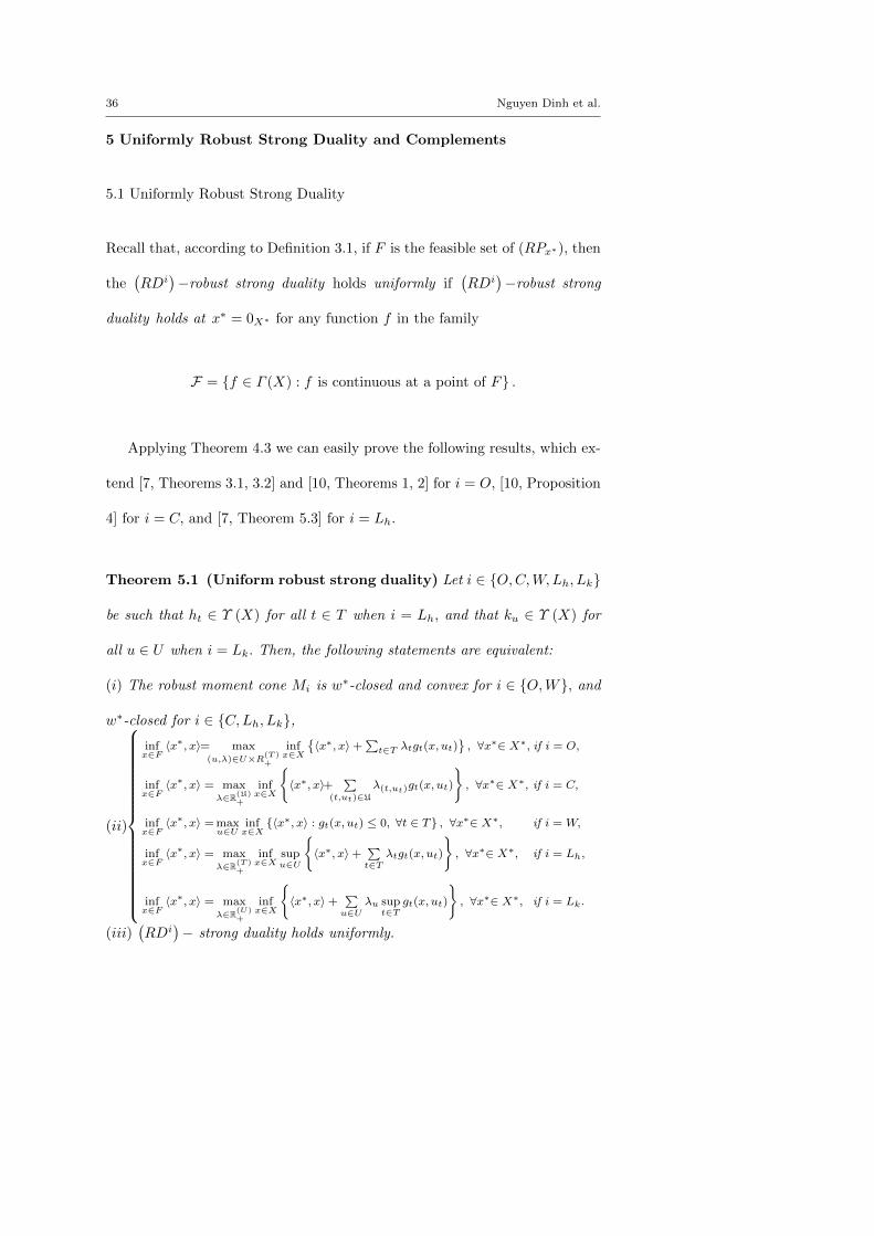
Theorem 5.1 (Uniform robust strong duality) Let i ∈ {O,C,W,Lh, Lk}
be such that ht ∈ Υ (X) for all t ∈ T when i = Lh, and that ku ∈ Υ (X) for
all u ∈ U when i = Lk. Then, the following statements are equivalent:
(i) The robust moment cone Mi is w∗-closed and convex for i ∈ {O,W}, and
w∗-closed for i ∈ {C,Lh, Lk},
(ii)
infx∈F〈x∗, x〉= max
(u,λ)∈U×R(T )+
infx∈X
{〈x∗, x〉+
∑t∈T λtgt(x, ut)
}, ∀x∗∈ X∗, if i = O,
infx∈F〈x∗, x〉 = max
λ∈R(U)+
infx∈X
{〈x∗, x〉+
∑(t,ut)∈U
λ(t,ut)gt(x, ut)
}, ∀x∗∈ X∗, if i = C,
infx∈F〈x∗, x〉 = max
u∈Uinfx∈X
{〈x∗, x〉 : gt(x, ut) ≤ 0, ∀t ∈ T} , ∀x∗∈ X∗, if i = W,
infx∈F〈x∗, x〉 = max
λ∈R(T )+
infx∈X
supu∈U
{〈x∗, x〉+
∑t∈T
λtgt(x, ut)
}, ∀x∗∈ X∗, if i = Lh,
infx∈F〈x∗, x〉 = max
λ∈R(U)+
infx∈X
{〈x∗, x〉+
∑u∈U
λu supt∈T
gt(x, ut)
}, ∀x∗∈ X∗, if i = Lk.
(iii)(RDi
)− strong duality holds uniformly.
Page 37
A Unifying Approach to Robust Convex Infinite Optimization Duality 37
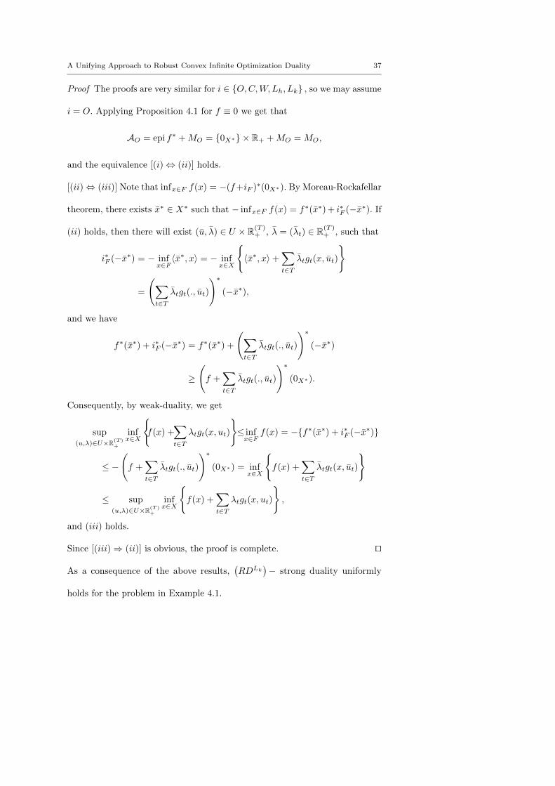
Proof The proofs are very similar for i ∈ {O,C,W,Lh, Lk} , so we may assume
i = O. Applying Proposition 4.1 for f ≡ 0 we get that
AO = epi f∗ +MO = {0X∗} × R+ +MO = MO,
and the equivalence [(i)⇔ (ii)] holds.
[(ii)⇔ (iii)] Note that infx∈F f(x) = −(f+iF )∗(0X∗). By Moreau-Rockafellar
theorem, there exists x∗ ∈ X∗ such that − infx∈F f(x) = f∗(x∗) + i∗F (−x∗). If
(ii) holds, then there will exist (u, λ) ∈ U × R(T )+ , λ = (λt) ∈ R(T )
+ , such that
i∗F (−x∗) = − infx∈F〈x∗, x〉 = − inf
x∈X
{〈x∗, x〉+
∑t∈T
λtgt(x, ut)
}
=
(∑t∈T
λtgt(., ut)
)∗(−x∗),
and we have
f∗(x∗) + i∗F (−x∗) = f∗(x∗) +
(∑t∈T
λtgt(., ut)
)∗(−x∗)
≥
(f +
∑t∈T
λtgt(., ut)
)∗(0X∗).
Consequently, by weak-duality, we get
sup(u,λ)∈U×R(T )
+
infx∈X
{f(x) +
∑t∈T
λtgt(x, ut)
}≤ infx∈F
f(x) = −{f∗(x∗) + i∗F (−x∗)}
≤ −
(f +
∑t∈T
λtgt(., ut)
)∗(0X∗) = inf
x∈X
{f(x) +
∑t∈T
λtgt(x, ut)
}
≤ sup(u,λ)∈U×R(T )
+
infx∈X
{f(x) +
∑t∈T
λtgt(x, ut)
},
and (iii) holds.
Since [(iii)⇒ (ii)] is obvious, the proof is complete. ut
As a consequence of the above results,(RDLk
)− strong duality uniformly
holds for the problem in Example 4.1.
Page 38
38 Nguyen Dinh et al.
5.2 Robust Duality for Convex Problems with Linear Objective Function
The robust counterpart with linear objective f(x) = 〈c∗, x〉, c∗ ∈ X∗, has the
form
(ROLP ) infx∈X〈c∗, x〉 s.t. gt (x, ut) ≤ 0, ∀(t, ut) ∈ U,
with corresponding robust dual problems
(ROLDO) sup(u,λ)∈U×R(T )
+
infx∈X
{〈c∗, x〉+
∑t∈T
λtgt (x, ut)
},
(ROLDC) supλ∈R(U)
+
infx∈X
{〈c∗, x〉+
∑(t,ut)∈U
λ(t,ut)gt (x, ut)
},
(ROLDW ) supu∈U
infx∈X{〈c∗, x〉 : gt (x, ut) ≤ 0, ∀t ∈ T} ,
(ROLDLh) supλ∈R(T )
+
infx∈X
supu∈U
{〈c∗, x〉+
∑t∈T
λtgt (x, ut)
},
(ROLDLk) supλ∈R(U)
+
infx∈X
supt∈T
{〈c∗, x〉+
∑u∈U
λuku (x)
}.
We now give a geometric interpretation of the optimal values of the above
five dual problems in terms of the corresponding moment cones.
Proposition 5.1 (Robust duality and moment cones)
Let i ∈ {O,C,W,Lh, Lk} be such that ht ∈ Υ (X) for all t ∈ T when i = Lh,
and that ku ∈ Υ (X) for all u ∈ U when i = Lk. Then,
sup(ROLDi) = sup {r ∈ R : − (c∗, r) ∈Mi} . (17)
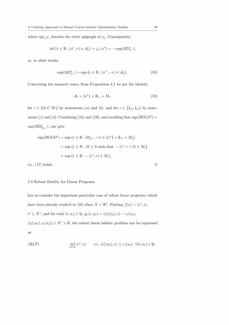
Proof Given i ∈ {O,C,W,Lh, Lk} , from the definitions of ϕi and Ai one gets
epis ϕi ⊂ Ai ⊂ epiϕi,
Page 39
A Unifying Approach to Robust Convex Infinite Optimization Duality 39
where epis ϕi denotes the strict epigraph of ϕi. Consequently,
inf {r ∈ R : (x∗, r) ∈ Ai} = ϕi (x∗) = − sup(RDix∗),
or, in other words,
sup(RDix∗) = sup {r ∈ R : (x∗,−r) ∈ Ai} . (18)
Concerning the moment cones, from Proposition 4.1 we get the identity
Ai = {c∗} × R+ +Mi, (19)
for i ∈ {O,C,W} by statements (a) and (b), and for i ∈ {Lh, Lk} by state-
ments (c) and (d). Combining (18) and (19), and recalling that sup(ROLDi) =
sup(RDi0X∗
), one gets
sup(ROLDi) = sup {r ∈ R : (0∗X∗ ,−r) ∈ {c∗} × R+ +Mi}
= sup {r ∈ R : ∃δ ≥ 0 such that − (c∗, r + δ) ∈Mi}
= sup {r ∈ R : − (c∗, r) ∈Mi} ,
i.e., (17) holds. ut
5.3 Robust Duality for Linear Programs
Let us consider the important particular case of robust linear programs, which
have been already studied in [10] when X = Rn. Putting f(x) = 〈c∗, x〉,
c∗ ∈ X∗, and for each (t, ut) ∈ U, gt(x, ut) = 〈x∗t (ut), x〉 − rt(ut),
(x∗t (ut), rt(ut)) ∈ X∗ ×R, the robust linear infinite problem can be expressed
as
(RLP ) infx∈X〈c∗, x〉 s.t. 〈x∗t (ut), x〉 ≤ rt(ut), ∀(t, ut) ∈ U.
Page 40
40 Nguyen Dinh et al.
It is easy to see that the corresponding moment cones are
MO :=⋃
u=(ut)t∈T∈Uconv cone {(x∗t (ut), rt(ut)), t ∈ T ; (0X∗ , 1)} ,
MC := conv cone {(x∗t (ut), rt(ut)), (t, ut) ∈ U; (0X∗ , 1)} ,
MW :=⋃
u=(ut)t∈T∈Ucl conv cone {(x∗t (ut), rt(ut)), t ∈ T} ,
MLh:= conv cone
⋃t∈T
cl conv
( ⋃ut∈Ut
{(x∗t (ut), rt(ut)) + R+(0X∗ , 1)} ; (0X∗ , 1)
),
MLk:= conv cone
⋃u∈U
cl conv
(⋃t∈T{(x∗t (ut), rt(ut)) + R+(0X∗ , 1)} ; (0X∗ , 1)
).
From (3),
inf(RLP ) = sup {r ∈ R : 〈c∗, x〉 ≥ r, ∀x ∈ F}
= sup{r ∈ R : − (c∗, r) ∈MC
}.
We also associate with problem (RLP ) the corresponding dual problems:
(RLDO) sup(u,λ)∈U×R(T )
+
infx∈X
{〈c∗, x〉+
∑t∈T λt(〈x∗t (ut), x〉 − rt(ut))
},
(RLDC) supλ∈R(U)
+
infx∈X
{〈c∗, x〉+
∑(t,ut)∈U
λ(t,ut)(〈x∗t (ut), x〉 − rt(ut))
},
(RLDW ) supu∈U
infx∈X{〈c∗, x〉 : 〈x∗t (ut), x〉 ≤ rt(ut), ∀t ∈ T} ,
(RLDLh) supλ∈R(T )
+
infx∈X
supu∈U
{〈c∗, x〉+
∑t∈T
λt(〈x∗t (ut), x〉 − rt(ut))},
(RLDLk) supλ∈R(U)
+
infx∈X
{〈c∗, x〉+
∑u∈U
λu supt∈T
(〈x∗t (ut), x〉 − rt(ut))}.
Proposition 5.2 Let i ∈ {O,C,W,Lh, Lk} be such that ht ∈ Υ (X) for all
t ∈ T when i = Lh, and that ku ∈ Υ (X) for all u ∈ U when i = Lk. Then, the
following statements hold:
Page 41
A Unifying Approach to Robust Convex Infinite Optimization Duality 41
(i) sup(RLDi) = sup {r ∈ R : − (c∗, r) ∈Mi} .
(ii)(RLDi
)− strong duality holds uniformly for any c∗ ∈ X∗ if and only
if the robust moment cone Mi is w∗-closed and convex for i ∈ {O,W}, and
w∗-closed for i ∈ {C,Lh, Lk} .
Proof (i) It follows immediately from Proposition 5.1.
(ii) It is a consequence of the equivalence [(i)⇔ (ii)] in Theorem 5.1. ut
An alternative proof of Proposition 5.2(i) for i ∈ {C,Lh, Lk} can be ob-
tained from [26, Lemma 4.3], by taking into account that (RLDC), (RLDLh)
and (RLDLh) are nothing else than the Lagrange dual problems corresponding
to linear representations of the feasible set of (RLP ) with characteristic cones
MC , MLh, and MLk
, respectively. Proposition 5.2(ii) generalizes [22, Theorem
8.4], where i = C and X = Rn.
Let us revisit Example 4.1. According to (17), sup(RLDi) = −‖c∗‖ ,
i ∈ {C,Lh, Lk} . We now check the fulfilment of (17) for i ∈ {O,W} . Given
(u, λ) ∈ U × R([0,1])+ ,
infx∈R2
{〈c∗, x〉+
∑t∈[0,1]
λt(〈x∗t (ut), x〉 − rt(ut))
}=
∑t∈]0,1]
λt(−t)− λ0(r0+1r0
)+ infx∈R2
{〈c∗, x〉+ λ0 ((cosα0)x1 + (sinα0)x2)}
=∑
t∈]0,1]λt(−t)− λ0
(r0+1r0
)+ infx∈R2〈c∗ + λ0(cosα0, sinα0), x〉,
and so
Page 42
42 Nguyen Dinh et al.
infx∈R2
〈c∗, x〉+∑t∈[0,1]
λt(〈x∗t (ut), x〉 − rt(ut))
=
∑
t∈]0,1]λt(−t)− λ0
(r0+1r0
), if c∗ = −λ0(cosα0, sinα0)
−∞, otherwise.
Therefore,
sup(RLDO) =
sup
(u,λ)∈U×R(T )+
{ ∑t∈]0,1]
λt(−t)− λ0(r0+1r0
)}, if c∗ ∈ −λ0D,
−∞, otherwise,
=
sup
λ∈R(T )+
{ ∑t∈]0,1]
λt(−t)− ‖c∗‖
}, if −c∗ ∈ R++D,
−∞, otherwise,
=
−‖c∗‖ , if − c∗ ∈ R++D,
−∞, else.
(observe that c∗ ∈ −λ0D with c∗ 6= (0, 0) entails that λ0 > 0, and so the
supremum of (RLDO) is not attained).
We now take u ∈ U. Eliminating redundant constraints, (Pu) can be ex-
pressed as
(Pu) infx∈R2〈c∗, x〉 s.t. (cosα0)x1+(sinα0)x2 ≤
r0 + 1
r0,
with
inf(Pu) =
−(r0+1r0
)‖c∗‖ , if (cosα0, sinα0) = − c∗
‖c∗‖ ,
−∞, else.
Thus, for i ∈ {O,W} , if −c∗ /∈ R++D, we have an infinite robust duality gap;
otherwise,
sup(RLDi) = min(RLP ),
Page 43
A Unifying Approach to Robust Convex Infinite Optimization Duality 43
i.e., we have (RLDi)−robust zero-gap (but not strong) duality. In fact, Ai is
closed and convex regarding {0x∗} × R if and only if Mi is closed and convex
regarding {−c∗} × R, which is not the case. Observe also that
sup {r ∈ R : − (c∗, r) ∈Mi} =
−‖c∗‖ , if −c∗ ∈ R++D,
−∞, else,
so that (17) holds for i ∈ {O,W} .
Finally, we observe that only(RLDLh
)enjoys uniform robust strong duality.
5.4 Reverse Robust Strong Duality
In addition to the main results on robust strong duality provided in the previ-
ous section, some results on reverse robust strong duality can be derived from
convex infinite duality, recently revisited in [27]. In fact, Theorem 5.3 below is
a slight adaptation of [27, Theorem 2] to robust case. Recall that a function
h ∈ Γ (X) is weakly-inf-locally compact when for each r ∈ R, the sublevel set
[h ≤ r] is weakly-locally compact (i.e., locally compact for the weak-topology
in X). We also denote by h∞ the recession function of h (whose epigraph is
the recession cone of epih).
Proposition 5.3 Assume that sup(RDC) 6= +∞, and additionally, the fol-
lowing conditions are fulfilled:
(a) ∃λ ∈ R(U)+ : f +
∑(t,ut)∈U
λ(t,ut)gt(., ut) is weakly-inf-locally compact,
(b) the recession cone of (RP ), namely
[f∞ ≤ 0]⋂ ⋂
(t,ut)∈U
[(gt(., ut))∞ ≤ 0]
,
Page 44
44 Nguyen Dinh et al.
is a linear space.
Then, min inf(RP ) = sup(RDC) and the optimal set of (RP ) is the sum of
a non-empty, weakly-compact and convex set and a finite dimensional linear
space.
In the same way, Theorem 5.4 below is a simple adaptation of [27, Theorem
3]. The topology on R(U) × R is the product topology.
Proposition 5.4 Assume sup(RDC) 6= −∞. Then, the following statements
are equivalent:
(i) min(RP ) = sup(RDC).
(ii)⋃
x∈dom f
(((gt(x, ut)
)(t,ut)∈U
, f(x)
)+(RU
+ × R+
)is closed regarding {0RU}×R.
6 The General Uncertain Problem
We consider in this last section the general uncertain problem
(Q)
{infx∈X{f(x, v) s.t. gt(x, ut) ≤ 0, ∀t ∈ T}
}(ut)t∈T∈U, v∈V
, (20)
where U =∏t∈T
Ut, V is another uncertainty set, which is a subset of some
lcHtvs, and f(., v) ∈ Γ (X), for all v ∈ V. This problem admits the following
pessimistic reformulation as an uncertain problem with deterministic objective
function (of the type studied in the previous sections):
(P )
{inf
(x,r)∈X×R{F (x, r) s.t. Gt(x, r, ut) ≤ 0, t ∈ T, H(x, r, v) ≤ 0}
}(ut)t∈T∈U, v∈V
,
where
F (x, r) := r, Gt(x, r, ut) = gt(x, ut) and H(x, r, v) = f(x, v)− r.
Page 45
A Unifying Approach to Robust Convex Infinite Optimization Duality 45
The totally explicit robust counterpart of (P ) is the problem
(RPC) inf(x,r)∈X×R
F (x, r) s.t.Gt(x, r, ut) ≤ 0, ∀(t, ut) ∈ U,
and H(x, r, v) ≤ 0, ∀v ∈ V,
,
where U := {(t, ut) : t ∈ T, ut ∈ Ut}.
The classical dual of the convex infinite problem (RPC) is
(RDC) supλ∈R(U)
+
µ∈R(V )+
inf(x,r)∈X×R
F (x, r) +
∑(t,ut)∈U
λ(t,ut)Gt(x, r, ut)
+∑v∈V
µvH(x, r, v)
.
According to the definition of the functions F, Gt and H, we easily obtain
(RDC) supλ∈R(U)
+ ,
µ∈R(V )+ ,∑
v∈Vµv=1
infx∈X
∑(t,ut)∈U
λ(t,ut)gt(x, ut) +∑v∈V
µvf(x, v)
.
We have
(Gt(., ., ut))∗(x∗, s) =
gt(., ut))
∗(x∗), if s = 0,
+∞, else,
epi(Gt(., ., ut))∗ = {(x∗, 0, θ) ∈ X∗ × R× R : gt(., ut))
∗(x∗) ≤ θ} ,
(H(., ., v))∗(x∗, s) =
f(., v))∗(x∗), if s = −1,
+∞, else,
epi(H(., ., v))∗ = {(x∗,−1, θ) ∈ X∗ × R× R : f(., v))∗(x∗) ≤ θ} .
Thus, the moment cone associated with (RPC) is
M ′C = conv cone
{(0X∗ , 0, 1)} ∪
⋃(t,ut)∈U {(x
∗, 0, θ) : gt(., ut))∗(x∗) ≤ θ}
∪⋃v∈V {(x∗,−1, θ) : f(., v))∗(x∗) ≤ θ}
.
Page 46
46 Nguyen Dinh et al.
Since
F ∗(x∗, s) =
0, if x∗ = 0X∗ and s = 1,
+∞, else,
we get epiF ∗ = {(0X∗ , 1)} × R+. Assuming that inf(RPC) 6= +∞, and ap-
plying Theorem 4.1 and Proposition 4.1, we conclude that
inf(RPC) = max(RDC) if and only if
{(0X∗ , 1)} × R+ +M ′C is closed regarding (0X∗ , 0)} × R.
7 Conclusions
In most applications of convex optimization, the data defining the nominal
problem are uncertain, so that the decision maker must choose among differ-
ent uncertainty models. Parametric models (stability and sensitivity analyses)
are based on embedding the nominal problem into a suitable topological space
of admissible perturbed problems, the so-called space of parameters. Sensitiv-
ity analysis provides estimations of the impact of a given perturbation of the
nominal problem on the optimal value while stability analysis provides con-
ditions under which sufficiently small perturbations of the nominal problem
provoke only small changes in the optimal value, the optimal set and the feasi-
ble set, as well as approximate distances, in the space of parameters, from the
nominal problem to important families of problems. Stochastic optimization,
in turn, assumes that the uncertain data are random variables with a known
probability distribution and provides either the probability distribution of the
optimal value under strong assumptions or its empirical distribution via simu-
Page 47
A Unifying Approach to Robust Convex Infinite Optimization Duality 47
lation. Both approaches to uncertain convex optimization, the parametric and
the stochastic ones, are considered unrealistic by many practitioners for which
it is preferable to describe the uncertainty via sets. Indeed, robust models as-
sume that all instances of the data belong to prescribed sets (the so-called
uncertainty sets), and select an ”optimal decision” among those which are fea-
sible under any conceivable data. Assuming that the optimal value function
f is deterministic, the robust decision makers agree in minimizing f on the
set of robust feasible solutions. In contrast with the existing unanimity of the
robust optimization community in solving this (pessimistic) primal problem,
there exists a variety of possible choices of its (optimistic) dual counterpart.
We have chosen in Sections 5 the so-called min-max robust counterpart, which
consists of minimizing the worst case for the objective function on the robust
feasible set.
This paper examines five different dual pairs in robust convex optimization
(two of them already known), each one based on a corresponding moment cone.
In particular, we characterize:
– Robust strong (or inf-max) duality in terms of the closedness regarding the
vertical axis of the corresponding moment cones.
– Uniform robust strong duality (i.e., the fulfilment of robust strong duality for
arbitrary convex objective functions) in terms of the closedness regarding the
whole space and the convexity of the moment cones.
Page 48
48 Nguyen Dinh et al.
– Robust reverse strong (or min-sup) duality in terms of the linearity of the
recession cone of the robust primal problem and the closedness of certain set
regarding the vertical axis.
Moreover, we analyze robust duality for convex problems with linear objec-
tive function x 7→ 〈c∗, x〉 and the particular case of robust linear optimization,
for which we provide results which are new even in the deterministic setting
(when the uncertainty sets are singleton), e.g., the characterization of the op-
timal value of the five dual problems in terms of the intersection of a vertical
line through the point (−c∗, 0) with the corresponding moment cone.
Acknowledgements The authors are grateful to the referees for their constructive com-
ments and helpful suggestions which have contributed to the final preparation of the paper.
This research was supported by the National Foundation for Science & Technology De-
velopment (NAFOSTED) of Vietnam, Project 101.01-2015.27, Generalizations of Farkas
lemma with applications to optimization, by the Ministry of Economy and Competitiveness
of Spain and the European Regional Development Fund (ERDF) of the European Com-
mission, ProjectMTM2014-59179-C2-1-P, and by the Australian Research Council, Project
DP160100854. Parts of the work of the first author were developed during his visit to the
Department of Mathematics, University of Alicante in July 2016, for which he would like to
express his sincere thanks to the support and the hospitality he received.
References
1. Ben-Tal A., El Ghaoui L., Nemirovski A., Robust Optimization, Princeton U.P., Prince-
ton (2009)
2. Gabrel V., Murat C., Thiele A., Recent advances in robust optimization: an overview.
European J. Oper. Res. 235, 471-483 (2014)
Page 49
A Unifying Approach to Robust Convex Infinite Optimization Duality 49
3. Beck A., Ben-Tal A., Duality in robust optimization: Primal worst equals dual best,
Oper. Res. Letters 37, 1-6 (2009)
4. Li G.Y., Jeyakumar V., Lee G.M., Robust conjugate duality for convex optimization
under uncertainty with application to data classification, Nonlinear Analysis 74, 2327-
2341 (2011)
5. Wang W., Fang D., Chen Z., Strong and total Fenchel dualities for robust convex opti-
mization problems, J. Inequal. Appl. 70, 21 (2015)
6. Suzuki S., Kuroiwa D., Lee G.M., Surrogate duality for robust optimization, European
J. Oper. Res. 231, 257- 262 (2013)
7. Jeyakumar V., Li G.Y., Strong duality in robust convex programming: complete charac-
terizations, SIAM J. Optim. 20, 3384-3407 (2010)
8. Jeyakumar V., Li G.Y., Robust duality for fractional programming problems with
constraint-wise data uncertainty, J. Optim. Theory Appl. 151, 292 - 303 (2011)
9. Jeyakumar V., Li G.Y., Lee G.M., Robust duality for generalized convex programming
problems under data uncertainty, Nonlinear Anal. 75, 1362-1373 (2012)
10. Goberna M.A., Jeyakumar V., Li G., Lopez M.A., Robust linear semi-infinite program-
ming duality under uncertainty, Math. Programming 139B, 185-203,(2013)
11. Jeyakumar V., Li G.Y., Srisatkunarajah S., Strong duality for robust minimax fractional
programming problems, European J. Oper. Res. 228, 331-336 (2013)
12. Jeyakumar V., Li G.Y., Wang J.H., Some robust convex programs without a duality
gap, J. Convex Anal. 20, 377-394 (2013)
13. Gorissen B.L., Blanc H., den Hertog D., Ben-Tal A., Technical note - deriving robust and
globalized robust solutions of uncertain linear programs with general convex uncertainty
sets, Oper. Res. 62, 672-679 (2014)
14. Jeyakumar V., Lee G.M., Lee J.H., Generalized SOS-convexity and strong duality with
SDP dual programs in polynomial optimization, J. Convex Anal. 22, 999-1023 (2015)
15. Wang Y., Shi R., Shi J., Duality and robust duality for special nonconvex homogeneous
quadratic programming under certainty and uncertainty environment, J. Global Optim.
62, 643-659 (2015)
Page 50
50 Nguyen Dinh et al.
16. Bot R.I., Jeyakumar V., Li G.Y., Robust duality in parametric convex optimization,
Set-Valued Var. Anal. 21, 177-189 (2013)
17. Sun X.-K., Chai Y., On robust duality for fractional programming with uncertainty
data, Positivity 18, 9-28 (2014)
18. Fang D., Li C., Yao J.-C, Stable Lagrange dualities for robust conical programming, J.
Nonlinear Convex Anal. 16, 2141-2158 (2015)
19. Dinh N., Mo T.H., Vallet G., Volle M., A unified approach to robust Farkas-type results
with applications to robust optimization problems, SIAM J. Optim. 27, 1075-1101 (2017)
20. Barro M., Ouedraogo A., Traore S., On uncertain conical convex optimization problems,
Pacific J. Optim. 13, 29-42 (2017)
21. Dinh N., Goberna M.A., Lopez M.A., From linear to convex systems: Consistency,
Farkas Lemma and applications. J. Convex Anal. 13, 279-290 (2006)
22. Goberna M.A., Lopez M.A., Linear Semi-infinite Optimization, Wiley, Chichester (1998)
23. Dinh N., Goberna M.A., Lopez M.A., Son T.Q., New Frakas-Minkowski constraint qual-
ifications in convex infinite programming, ESAIM: COCV 13, 580-597 (2007)
24. Sion M., On general minimax theorems, Pacific Journal of Mathematics. 8, 171–176
(1958)
25. Goberna M.A., Lopez M.A., Volle M., Primal attainment in convex infinite optimization
duality, J. Convex Anal. 21, 1043-1064 (2014)
26. Goberna M.A., Jeyakumar V., Lopez M.A., Necessary and sufficient constraint qualifi-
cations for systems of infinite convex inequalities, Nonlinear Analysis 68, 1184-1194 (2008)
27. Goberna M.A., Lopez M.A., Volle M., New glimpses on convex infinite optimization
duality, Rev. R. Acad. Cien. (Serie A. Mat.) 109, 431-450 (2015)