A v Fermi National Accelerator Laboratory

TM-1519

RF Cavity Primer for Cyclic Proton Accelerators'

James E. Griffin Fermi National Accelerator Laboratory P.O. Box 500, Batavia, Illinois 60510

April 1988

*Presented at the INFN ELOISA TRON Project 4th Workshop: Very High Energy Proton-Proton Physics, Ettore Majorana Center for Scientific Culture, Erice-Trapani, Italy, May 31-June 7, 1987

:Q: Operated by Universities Research Association Inc. under contract with the United States Department or Energy

1

RF CAVITY PRIMER FOR CYCLIC PROTON ACCELERATORS

ABSTRACT

James E. Griffin

Fermi National Accelerator Laboratory Batavia, Illinois 60510 U.S.A.

This report contains the substance of lectures on fundamentals of proton accelerator rf systems presented at an Eloisatron Workshop, Ettore Majorana Center, Erice, Italy, in May, 1987.

INTRODUCTION

The purpose of this note is to describe the electrical and mechanical properties of

particle accelerator rf cavities in a manner which will be useful to physics and engineering graduates entering the accelerator field. The discussion will be limited to proton (or an­ti proton) synchrotron accelerators or storage rings operating roughly in the range of 20 to 200 MHz. The very high gradient, fixed frequency UHF or microwave devices appropriate for electron machines and the somewhat lower frequency and broader bandwidth devices required for heavy ion accelerators are discussed extensively in other papers in this series.

While it is common practice to employ field calculation programs such as SUPERFISH, URMEL, or MAFIA as design aids in the development of rf cavities, I,2,3 we attempt here to elucidate various of the design parameters commonly dealt with in proton machines through the use of simple standing wave coaxial resonator expressions. In so doing, we treat only standing wave structures. Although low-impedance, moderately broad pass-band travelling wave accelerating systems are used in the CERN SPS, 4 such systems are more commonly found in linacs, and they have not been used widely in large cyclic accelerators.

Two appendices providing useful supporting material regarding relativistic particle dynamics and synchrotron motion in cyclic accelerators are added to supplement the text.

ACCELERATOR REQUIREMENTS

Before proceeding with a detailed description of rf cavities, it will be useful to develop some ideas of the requirements and limitations imposed on the designs by the general proper­ties of the accelerators in which they are to be used.

2

Physical Size, Apertures

Proton synchrotron accelerator complexes usually consist of a series of accelerators operating over a sequence of energy ranges. Protons or H- ions are injected into the first synchrotron from a linear accelerator at an energy between 100 and 1000 Me V. Because of practical limitations on the range over which useful bending magnetic fields can be developed, the momentum range of each successive synchrotron is limited to about 30: !. A further limitation on the momentum range of the first ring may arise because of the cost balance between providing the bending magnet length required for the highest momentum and the magnet size required to provide the physical aperture for the injected beam.

We assume, for example, that the first ring in the sequence spans a momentum range of 12.5:1, carrying protons from 1.696 to 21.2 GeV/c. (Useful relationships between kinetic energy, total energy, velocity, momentum, ~, y, and electrical forces on protons are devel­oped in Appendix A.) This ring uses iron core magnets with a maximum useful bending field of 1.5 T developing a bending radius at maximum momentum of 47.1 m. A total bending magnet length of 296 meters is required to deflect the beam by 2 1t radians. The actual orbit length must be increased substantially to allow space for focussing quadrupole magnets, higher order correction magnets, injection and extraction devices, diagnostic equipment, and finally, rf accelerating cavities. The total circumference of such a machine would be near 500 m, with, perhaps, 120 m available for rf cavities.

The next ring in the sequence could carry protons from 21.2 to about 500 Ge Vic with a circumference of about 7500 m. At least 100 m of circumference would be available for rf equipment. Following this ring one might find a large ring of 8 - 10 T superconducting magnets sustaining a maximum energy of 30 TeV and a circumference approaching 80 km.

The required apertures, or beam pipe sizes, in these machines might reasonably start at 6 by 10 cm at the lowest energy, decreasing to a 4 cm circular aperture at the highest energy.

Frequency Range, Frequency, Harmonic Number

At the lowest injection energy, 1 GeV, ~ = 0.875. With the proposed circumference of 500 m, protons require 1.9 microseconds to complete one turn; the rotation frequency is 524.65 kHz. At the extraction momentum, 21.2 GeV/c, ~has increased to 0.99902, and the rotation frequency is 599 kHz. The rf system could, in principle, operate at exactly these frequencies, swinging about 15 percent during acceleration. In fact, there are compelling reasons to operate at much higher frequencies, related to the rotation frequencies by an integer harmonic number h. Modern proton facilities have been operating at rf frequencies between 30 MHz (Fermilab, Petra-II) and 200 MHz (SPS, HERA). The choice is related to the frequency modulation requirements, the method of transfer of beam from one machine to

3

the next, and the beam bunch composition desired in the final very high energy ring. In the case at hand, it is reasonable to choose for the first ring a harmonic number h= 100 so that the rf frequency must swing from 52.46 to 59.9 MHz during acceleration.

The second ring in the sequence would operate over the very narrow frequency range 59.9 to 59.96 MHz at a harmonic number h=1500. The third ring operates at constant fre­quency 59.96 MHz, or possibly twice or four times that frequency at h=l6000, 32000, or 64000.

In the lowest energy ring the magnetic guide field ramp during acceleration will prob­ably be the independent variable and the rf frequency will have to be tuned to keep the beam at some mean radius within the aperture. This means that the rf system will have to be electrically tunable, almost certainly using the variability of ferrite magnetic permeability to tune the rf cavities. Until recently Ni-Zn Iron spine! ferrite would have been used, limiting the maximum frequency to about 60 MHz. Recently there have been developments5,6 using very low loss yttrium garnet ferrite for this purpose. The frequency range of cavities tuned in this manner may be increased to a few hundred MHz.

RF Voltage and Power

We are considering here rf systems whose only function is to develop a time varying electric field along the direction of motion of protons. Because these fields are varying (usually sinusoidally) synchronously with the rotation period, the energy gain of a particular proton may be positive, negative, or zero, depending upon its time of passage through the rf field. (We assume here that the rf fields are developed across gaps in the beam pipe which are short with respect to an rf wavelength and that the proton gap crossing time is short with respect to an rf period. The "transit time factor" is unity.7 This is not true in all ac­celerators.) The change in energy resulting from a single passage through the rf accelerating system will cause a change in rotation period of the particle so that subsequent crossings will occur at progressively different times. A detailed discussion of this "phase motion" is given in Appendix B.

The alternating fields confine the circulating proton beam into localized groups or "bunches." The bunches contain protons spanning a range of energy around a "synchronous energy" and span a phase or time period which is a fraction of one rf period. The bunches are centered around some phase angle, <l>s which depends on the static or dynamic conditions

of the synchrotron bending magnetic field.* A machine with harmonic number h can sustain

*This confinement principle of phase stability was first stated by V. I. Veksler in 1944 and independently by E. M. McMillan very shortly thereafter.

4

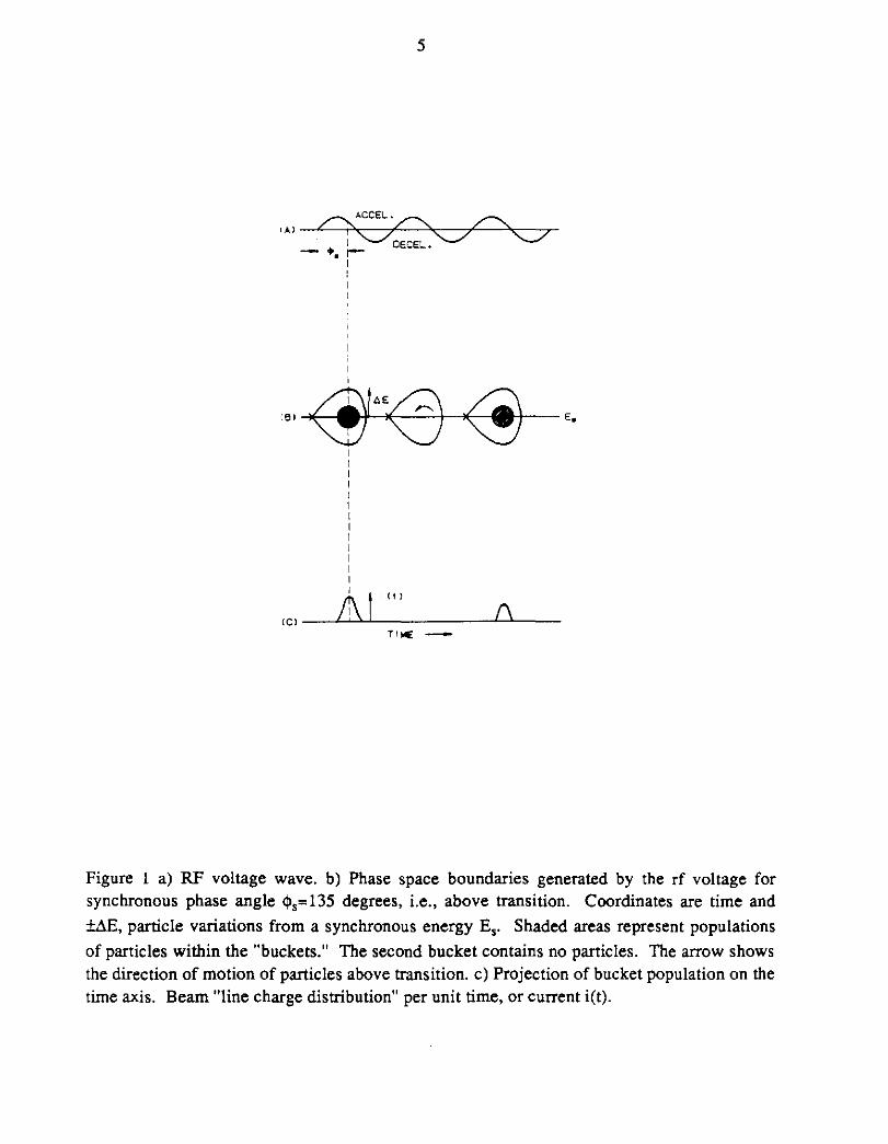
h such bunches although there need not be a bunch located on each rf wave (i.e., all bunches need not contain the same number of particles. See Figure 1.). If the magnetic bending field is increased or decreased, the average phase angle at which particles cross the accelerating gaps must be changed so that the average particle momentum will be that required to main­tain an orbit centered in the beam pipe. Here net energy must be delivered to or removed from the beam by the rf system.

In order to calculate the required rf voltage and the power which the rf system must deliver to the proton beam, we must propose more details for the hypothetical machines under consideration. Let us assume that the 1 Ge V linac delivers 24 ma of H- ions with an energy spead of ±1 MeV to a stripping foil in the injection channel of the Booster ac­celerator. If injection is allowed to proceed for seven turns, or 13.3 µs, a total of 2 x 1012 particles will be injected on each acceleration cycle.

The product of the total injected energy spread and the rotation period yields lon­gitudinal emittance of 3.S eV-s or 0.03S eV-s per rf wave, since hdOO. Using equations SB and SC, Appendix B, we find that an rf voltage slightly larger than 61 kV must be applied just following injection in order to create the required "bucket area" to bunch the beam. This voltage should be developed "adiabatically"B in order to minimize an unwanted increase in the longitudinal emittance during bunching. Alternatively, the rf voltage might be applied in advance of injection and previously bunched bursts of beam, created in the linac, may be "painted" into the existing buckets to provide a desired beam charge distribution. In such a case the required voltage would be substantially larger, a few hundred kV, depending on details of painting. During this injection period the rf system is delivering no net energy to the beam.

For acceleration the rf system must, in addition to creating bucket area, provide ac­celerating voltage and deliver energy to the beam. The accelerating voltage and power depend on details of the rate of acceleration. For the example being developed we assume that the Booster magnetic field time dependence (equivalent to the beam momentum time dependence) will consist of a 15 Hz Sine wave. The beam momentum dependence is

cp(t) = 11.44 - 9.75 cos(30m) GeV/c (1)

where tis in seconds. The beam momentum is changed from 1.69 to 21.l GeV/c in 33.33 ms. The rate of change of momentum reaches a maximum of 919 GeV/cs at 16.67 x l0-3s. The rate of change of momentum is equal to the net force exerted by the rf electric field which, averaged over one turn, is the rf voltage per turn seen by a particle, divided by the orbit length

5

(A) 0ACCEl.~ ~

I I "7 DECEL. ""7 ""7 --4 +. r--

1

' I

'

e1@1A~<J I@ E0

I

I I I I .,

I I I I I

I

I

A I "" <Cl-~-~~--------(\~--T 11€

Figure 1 a) RF voltage wave. b) Phase space boundaries generated by the rf voltage for synchronous phase angle $,= 135 degrees, i.e., above transition. Coordinates are time and

UE, particle variations from a synchronous energy E,. Shaded areas represent populations

of particles within the "buckets." The second bucket contains no particles. The arrow shows the direction of motion of particles above transition. c) Projection of bucket population on the time axis. Beam "line charge distribution" per unit time, or current i(t).

~ _ V sin <l>s dt - 2rrR

6

V sin <I> = 2rrR d (pc) = _l d (pc) s c dt F~ dt (2)

where F00 is the rotation frequency of a particle having velocity c, (in the Booster case, - 600

kHz). The required rf accelerating voltage at the maximum slope points is l .5MV per turn.

The required peak voltage depends on the synchronous phase angle <l>s which, in turn,

depends on the required bucket area through the moving bucket factor. 9•1° For constant rf voltage, the bucket area is minimum at 1.732 times the transition point. For the example at hand we may take Yt = 7 so the bucket area is minimum at 16.66 ms, the maximum slope

point. We may assume that a bucket area of 0.06 eV-s is required at this time in the cycle yielding a synchronous phase angle of 67 degrees and a peak rf voltage of 1.63 MV.

Note that by adding about 18 percent of second harmonic to the magnetic field at the proper phase, the momentum slope could be reduced to a minimum, requiring only about 1 MV of rf voltage for the above Booster example.

The maximum energy gain of 1.5 Me V per turn per particle is 1.2 x 1 o-7 Joules per second per particle or 240 kW for 2 x 1012 particles. This is the peak power which must be delivered to the beam by the booster rf system. The rf system must operate for about 35 ms out of each 67 ms acceleration period delivering an average power of 100 kW to the beam.

We assume that the next ring in the series is filled with 14 booster batches (2.8 x 1013 protons) and accelerates at a rate of 100 GeV/s. This requires the rf system to deliver 448 kW peak power to the beam at an accelerating voltage of 2.5 MV per turn. If the ring is assumed to have Yt near 18, a few kV of additional rf voltage is required to create an adequate

bucket area, about 0.08 eV-s. During injection and extraction, when the synchronous phase angle is zero, a minor difficulty may rise in creating sufficiently low rf voltages to avoid the generation of excessively large buckets which might result in undesired beam phase space dilution.

The 80 kM ring will require about 5 MV of rf voltage at constant frequency in order to accelerate to 30 TeV in about 1500 seconds. The required bucket area can be generated with a few tens of kV so the synchronous phase angle will be quite large. At a total beam inten­sity of 2 x 1014 protons, the rf system must provide about 600 kW to the beam during acceleration.

7

Beam Loading

The beam passing through the rf cavities, bunched as shown in Figure 1, will have a component of rf current at frequency f,r = hF0 between one and two times the de beam

current. This factor depends on the bunch shape, or line charge density distribution, and it may be determined by evaluating the normalized Fourier transform of an average bunch distribution at frequency hF0 and multiplying by twice the de current. In the example

Booster, at 590 kHz, the rf beam current at h=lOO would be about 0.3A.

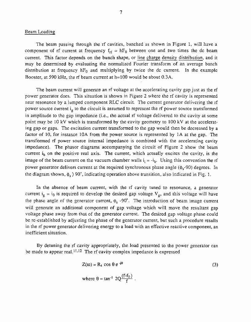
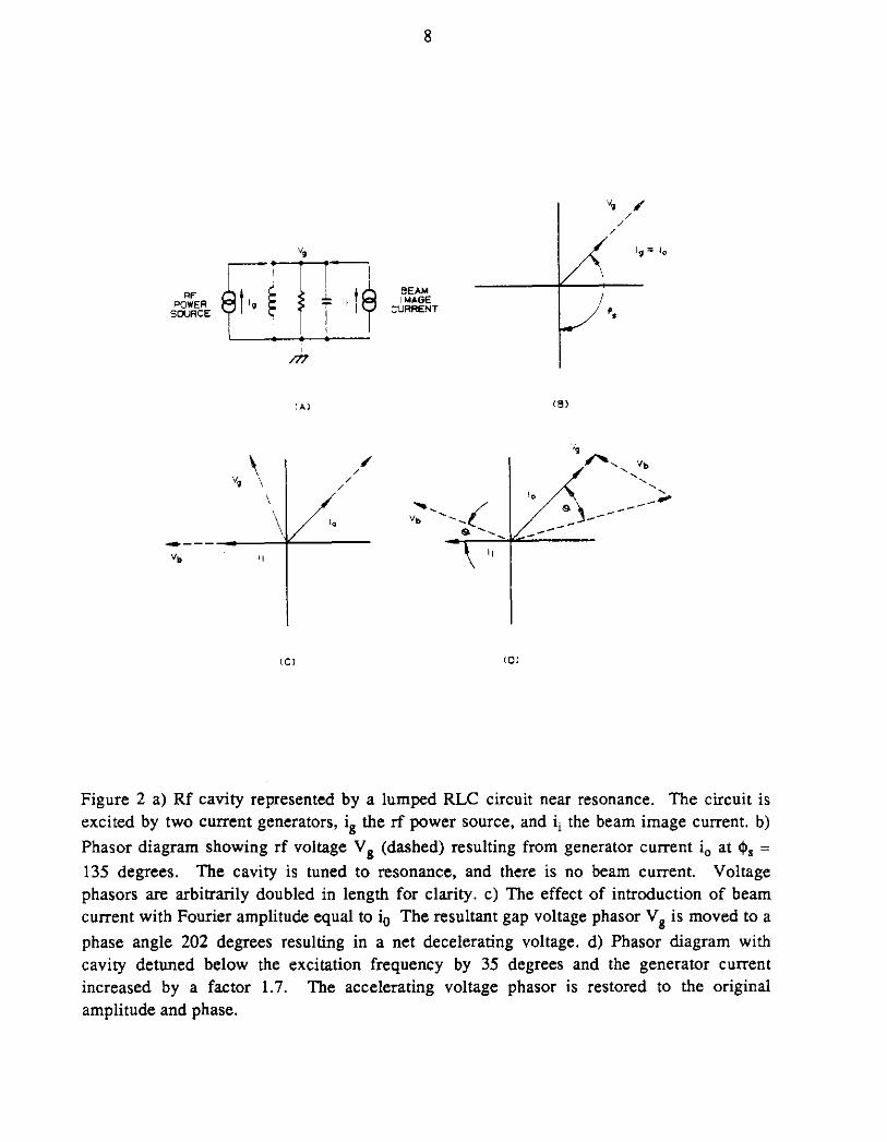
The beam current will generate an rf voltage at the accelerating cavity gap just as the rf power generator does. This situation is shown in Figure 2 where the rf cavity is represented near resonance by a lumped component RLC circuit. The current generator delivering the rf power source current ig to the circuit is assumed to represent the rf power source transformed

in amplitude to the gap impedance (i.e., the actual rf voltage delivered to the cavity at some point may be 10 kV which is transformed by the cavity geometry to 100 kV at the accelerat­ing gap or gaps. The excitation current transformed to the gap would then be decreased by a factor of 10, for instance lOA from the power source is represented by lA at the gap. The transformed rf power source internal impedance is combined with the accelerating cavity impedance). The phasor diagrams accompanying the circuit of Figure 2 show the beam current ib on the positive real axis. The current, which actually excites the cavity, is the

image of the beam current on the vacuum chamber walls i; = -ib. Using this convention the rf

power generator delivers current at the required synchronous phase angle (<jl,-90) degrees. In

the diagram shown, 4>,) 90°, indicating operation above transition, also indicated in Fig. 1.

In the absence of beam current, with the rf cavity tuned to resonance, a generator current ig = i0 is required to develop the desired gap voltage V g• and this voltage will have

the phase angle of the generator current, 4>, -90°. The introduction of beam image current

will generate an additional component of gap voltage which will move the resultant gap voltage phase away from that of the generator current. The desired gap voltage phase could be re-established by adjusting the phase of the generator current, but such a procedure results in the rf power generator delivering energy to a load with an effective reactive component, an inefficient situation.

By detuning the rf cavity appropriately, the load presented to the power generator can be made to appear rea[.11,12 The rf cavity complex impedance is expressed

Z(co) = R, cos 8 e -i0 (3)

where e = tan·1 2Q (f-:o) .

8

v, ,,, /

/ /

v, lg::: 10

! r__,1 RF I '• ~ f t ,,!~

BEAM I POWER IMAGE

SOURCE CURRENT '•

' m

IAI 1ei

.,

v, \

,,, /', vb / ' ' / ' / ' I '• '

s --__ _..

'• ---~---

v. ,,

ICJ <OJ

Figure 2 a) Rf cavity represented by a lumped RLC circuit near resonance. The circuit is excited by two current generators, i8 the rf power source, and ii the beam image current. b)

Phasor diagram showing rf voltage V 8 (dashed) resulting from generator current i0 at «!>, =

135 degrees. The cavity is tuned to resonance, and there is no beam current Voltage phasors are arbitrarily doubled in length for clarity. c) The effect of introduction of beam current with Fourier amplitude equal to io The resultant gap voltage phasor V 8 is moved to a

phase angle 202 degrees resulting in a net decelerating voltage. d) Phasor diagram with cavity detuned below the excitation frequency by 35 degrees and the generator current increased by a factor L 7, The accelerating voltage phasor is restored to the original amplitude and phase.

9

The detuning required to compensate for the beam current is expressed

Af _ ( R, ) hFo ib coscj>, u I - Q 2 Vg .

(4)

(5)

In order to preserve the magnitude of the required gap voltage, the generator current must be increased in the presence of beam current,

(6)

The beam loading compensation scheme described here requires two feedback systems operating on the rf cavity and power source system. One feedback loop adjusts the delivered power such that the generator current develops the desired gap voltage while the other loop controls the cavity tuning (or detuning), such that the load presented to the power source appears real under all conditions of beam current.

Beam Stability

The rf cavities will inevitably present impedances at the accelerating gap, in which rf frequency components of the beam current can induce voltages. Such induced voltages will react back on the beam in a manner which may cause unwanted synchrotron motion, usually referred to an longitudinal instability. 13 Such instabilities may cause an unwanted increase in the longitudinal emittance, (essentially bunch length and momentum spread), resulting in undesirable beam configuration for injection into a succeeding machine or experimental use. In severe cases such instability may result in beam loss. Instabilities caused by rf system impedances can be broken into two classes; those that are associated with the fundamental operating frequency, and those that result from spurious impedances at other frequencies. Instabilities associated with the fundamental rf operating frequency are usually termed Robinson instability.14,lS Coherent longitudinal oscillation of the beam bunched about the synchronous phase angle cause the appearance of frequency modulation sidebands adjacent to the rf frequency component of beam current. The largest of these sidebands are separated from the rf frequency by the synchrotron frequency (cf. Appendix B), usually a few hundred Hz to a few kHz. These current components induce voltages in the rf cavity impedance. If the cavity is tuned slightly off resonance, the real component of impedance will be different for the upper and lower sidebands, and the difference in amplitude of these two excitations creates a driving term or a damping term for the coherent synchrotron motion. Stability against this form of coherent bunch motion can be established by tuning the rf cavity system off resonance in such a way that the damping term dominates. If a machine is being operated below transition, stability is obtained by tuning the rf system slightly above the excitation

10

frequency so that the resistive component at the upper sideband is larger than that at the lower sideband frequency. Above transition, detuning below the excitation frequency is required. Fortunately, the direction of detuning to establish Robinson stability is the same as that required to compensate for beam loading.

There is another aspect to Robinson instability which amounts physically to the effect that coherent bunch synchrotron oscillation reacts on the rf system in such a way as to reduce the bucket area. The amount of reduction is governed by the ratio of power delivered to the beam to that dissipated in the rf system. When this ratio is equal to ~· the bucket area is reduced to zero and all beam will be lost if this happens during acceleration. Of course, the power delivered to the beam is proportional to the amount of beam in the machine so this effect is a beam self-limiting one, in that beam may be lost due to bucket area reduction until the power ratio is reduced to unity. This aspect of the Robinson instability can be eliminated by adjusting the shunt impedance of the rf system, and hence the internal power dissipation, until the internal dissipation is equal to or greater than the power delivered to the beam. In the Booster example the rf system would be required to dissipate 240 kW at a total gap voltage (all cavities) of 1.5 MV. The total shunt impedance should then be less than 4.7M­Ohm.

The Robinson instability relationships were developed considering rf cavities with no feedback control on the phase or amplitude of the gap voltage. The internal power dissipa­tion requirement can be reduced substantially by application of various forms of feedback around the rf cavity-power-amplifier system, the effect of which would be to reduce the effective gap, or output, impedance of the rf system as seen by the beam. With appropriate feedback in place the beam to cavity power ratio can, in principle, be increased by an order of magnitude. Ratios of 2: 1 have been achieved in practice. While this technique can reduce the total power dissipation and operating cost, it may not substantially reduce the size and cost of the rf power amplifier because, in order to develop the required low output im­pedance, the amplifier must be capable of delivering substantial power in transient situations to counteract the effects of beam excitation as it happens.

Coupled Bunch Instability

The bunches in a machine are capable of individual non-coherent longitudinal oscilla­tions within their individual buckets. Frequently the motion is such that all bunches oscillate with roughly the same amplitude with a progressive phase difference advancing through the successive bunches, completing 2mit radians around the machine. In other cases, a few bunches oscillate with large amplitude while others remain stable. In any case such motion, when Fourier analyzed, can display a spectrum of beam rf currents at harmonics of the rotation frequency plus or minus the synchrotron frequency. The amplitude of these spectral lines is again governed by the shape of the Fourier transform of an average individual bunch

11

and substantial amplitudes may be generated up to about 1 GHz by bunches a few ns in length. Real components of impedance at any frequency within the spectral range may be excited by these beam currents, and if the voltage generated is sufficiently high, the bunch motion responsible for a particular frequency may grow in amplitude. Therefore, it is ex­pedient to minimize the amplitude of gap shurt impedance created by spurious resonances in all rf cavities. Specific requirements depend on machine details and anticipated beam in­tensity, but generally, reduction of spurious shunt impedances to a few tens of kOhms is sufficient. These reductions are frequently done by special traps or networks within the cavities which are designed to avoid coupling large amounts of energy from the fundamental operating mode. Such traps are usually terminated in resistances or composed of resistive material which transforms a low impedance to the accelerating gap at selected frequencies.

The magnitude of the real component of impedance above which an instability may arise is related to machine parameters, beam current and beam momentum spread roughly as 16,17

(7)

where the constant, (around 3), is related to the beam charge distribution within the bucket and ib(n) is the beam current component at frequency nF0. The limiting value of R/n may

range from a few to a few hundred ohms.

RF Cavity R/Q

Beam stability requirements may place a limit on the ratio of shunt resistance to Q (quality factor) for the entire rf system at the fundamental operating frequency. In a large machine with a very low rotation frequency and large harmonic number, the two rotation harmonics adjacent to the rf frequency (h±l)F0 are very close to the operating frequency hF0.

At large beam intensity the beam loading cavity detuning, Eq. 5, will cause the impedances at the adjacent sidebands to become unequal, and it may raise the larger of the two to an amplitude capable of causing an m=l coupled bunch instability. Therefore, the real compo­nent of cavity impedance must be kept below K(h±l) = Kh (his large) at frequencies Fo(h±l).

From Eq. 3, the real component of cavity impedance is

R(f) = R, cos2 S R,

R, (8)

12

From Eq. 5, the cavity is already detuned by i\.f1, so i\.f in Eq. 8 becomes

(9)

Because the detuning condition, i\.f1, is largest at injection or extraction, when V g is small

and cp,=0, we set coscp, = 1. Combining Eqs. 8 and 9 we arrive at a sort of limiting condition

on R/Q. 2

R,!Q < 112

( ~) + ibh KR, Vg

(10)

In the 7500 m ring example, if the beam cavity power ratio is 2: I, the injection voltage 200 kV, and the beam stability limit K=3 Ohms, then R/Q is limited to about 186 Ohms. For

Kaon factory rings, where the beam current may be an order of magnitude higher, the R/Q limitation becomes more severe.

Transient Beam Loading

During the bunch-to-bucket beam transfer of several batches of beam, there are periods when the larger ring is partially full. In order for the beam loading compensation system to operate correctly in this situation, the feedback loops would require bandwidth sufficient to generate corrections in a few rf periods, usually not feasible. Frequently the rf cavity time constant, a = co/2Q, is several rotation periods so the voltage developed by bursts of current in the partially filled ring can be written

v(t) = (i\.i) Zc(Ol) [1-e·(~+jro)t]

= (i\.i)Zc (co) (a+jco)t

_ . (i\.i)co ( R,) = (i\.1)R, at= - 2- Q t.

(11)

Since these voltage excursions are, during the early transient period, in phase with the beam image current, they are in quadrature with the required gap voltage, when cp 5 is either zero or

n. The phase excursions, easily obtained from the gap voltage and Eq. 11, will cause selec­tive phase space dilution if not compensated. Frequently some form of feed-forward com­pensation is employed, but high precision is difficult. It is clear that reduction of RIQ is beneficial.

13

Vacuum and Radiation Environment

The design of each rf cavity must be such that appropriate vacuum can be maintained in the accelerating gap region. The required pressures would be 10-s - J0-9 T in the first two rings and perhaps 10-10 - 10-11 Tin the very large ring.

The rf equipment which is to be operated within the accelerator enclosure must be designed to operate satisfactorily for long periods in a region of substantial ionizing radiation flux. Accumulated radiation doses of 1 MRad per year of x-ray and light charged particles and I 013 neutrons/cm2 per year should be anticipated. Operational dose rates may be 300-500 Rad/h. In addition to satisfactory operation, rf equipment should be designed so that maintenance can be accomplished easily and expeditiously since it must be done in a signifi­cant residual radiation environment.

The insulating material used to isolate the accelerator vacuum from other parts of the rf syst~m, thus serving as an r.f.window, must be made of material whose electrical loss proper­ties are very good initially and will not deteriorate excessively under the radiation flux anticipated.

In addition to the above requirements, components of the rf cavities, such as insulating material, should not be made of materials which may emit noxious smoke into the accelerator enclosure in the event of electrical breakdown.

RF CAVITY GEOMETRIES

Simple Coaxial Structure Properties

The longitudinal electric fields required of the rf system can be developed by enclosing the beam pipe and its accelerating gap by a shorted coaxial structure as shown in Figure 3a. The inner conductor of the coaxial structure may be larger than the accelerator beam pipe and need not be made of the same material. The electrical properties of coaxial structures are widely known,18,19 and we intend only to develop a few useful relationships here.

The inductance per unit length (ignoring magnetic fields within the conductors) is

Henrys per meter.

The capacitance per unit length between inner and outer conductor is

Ci _ 21t Eo Er - In (r2 /rl) Farads per meter.

( 12)

(13)

9)

14

:

I '2

~·~ =o ! '· E

~ A l

0

I I '-- CERAMIC 'I ACUUM SEAL. ANO

=!F W 1 NQOW

<Bl

CCI

F!ELO FREE YOLUME

CEAAMIC SEAL.

Figure 3 a) a gap in the metallic beam pipe is formed into an accelerating resonator by enclosing the region with a shorted outer coaxial conductor. b) the physical length of the structure may be reduced without raising the frequency by adding lumped capacitance at the accelerating gap. In this case the capacitance is further increased by the presence of a ceramic cylinder which serves as an rf window and vacuum seal. c) The impedance transfor­mation ratio between the low impedance excitation point and the accelerating gap can be affected by varying the characteristic impedance of the structure along its length. This also may facilitate removal of the ceramic window to a point of lower electric field, as shown.

15

The resistance per unit length is:

Ohms per meter (14)

where p, = (itfµlcr) is the surface resistivity resulting from skin effect, and a is the bulk

conductivity of the material. At 60 MHz Ps is about 2 x 10·3 Ohms per square for high

conductivity copper and about 25 percent higher for aluminum. We will ignore real conduc­tance, G, between inner and outer conductor since the structure is usually air filled or evacuated.

Coaxial transmission lines support travelling TEM waves of the form

A (z,t) = Aeiwt·yz (15)

where A is the amplitude of a voltage, current, electric, or magnetic field, and y = o + j~ is a propagation constant consisting of a spatial attenuation term and a spatial phase constant. For the low loss structures under consideration (R << wL, G:=o)

(16)

[LC l l/2 [ ]l/2 2Jt p = w 1 1 = W µoEo = T (17)

where A. is the free space wavelength of waves with angular frequency w. In regions of a structure containing ferrite, or large amounts of dielectric material, the definition of~ should include the relative permeability or permitivity of the materials.

The travelling waves in the structures can be combined to form standing waves whose amplitudes and phases combine to meet the boundary conditions imposed by open circuits (at the accelerating gap) or short circuits at the shorted end of the structure. These boundary conditions are, of course, idealizations, since the open circuit will consist of some shunt capacitance in parallel with a real conductance and the "short" may have series resistance and inductance. For the idealized boundary conditions the spatial and time variations in voltages and currents, or electric and magnetic fields, will be shifted in phase with respect to each other by 90 degrees when the cavity is operated at, or near, resonance. Given this condition, it is no longer necessary to include eiWt in each expression. Maximum amplitudes of voltage and current are related through the characteristic impedance of the structure

16

Z: = [R1.+jmL1 )112 = [L1 )

112 (l _ ·~) JC!lC1 C1 J 2coL

(18)

If voltage and current are known at any point in the system, they may be calculated at any other point using the transfer matrix expression

( ~(z) )-( cosh(yz) z,sinh(yz) ) ( v(O)) 1(z) - smh(yz) cosh(yz) 1(0) z,

(19)

It is almost always valid to neglect losses when relating voltages and currents within an accelerating cavity. So, defining R0 = [L1/C1]112 as a real characteristic impedance, the

expression can be written

( v(z)) ( rnsBz jR0 sin(Bz) ) ( v(O)) i(z) = j smPz cos(Bz) i(O) ·

I<c (20)

If the radical E field and thereby, the voltage, at the shorted end of the line is assumed to be zero, and a current Io is assumed, then the voltage and current distributions along the line are

I(z) = Io cos~z, and

V(z) = jI0 Rc sin~z.

For line length D the gap voltage and the short end current are related by

Yg 'R . rlD r;;- =J ,sm.., .

Ignoring losses, the impedance at the open end is

Z;. = iRc tan~D.

(21)

(22)

(23)

Moving the open end gap around onto the beam pipe and additional structure in that region, such as a ceramic vacuum seal with field limiting corona rolls, will create a concentration of electric field in the gap region which is accounted for by a lumped gap capacitor Cg. The

admittance of the parallel combination of the lumped gap capacitance and the shorted coaxial line is

Y = [ ~~~] + j(CllCg - Y, cot~D). (24)

17

where Y c = Rc,1 and the real part of Y is created by losses in the line and possibly in the gap

capacitance. Parallel resonance (or "anti-resonance") occurs when the imaginary part of the input admittance is zero, at which point the magnitude of the input impedance is maximized and the time averaged electric and magnetic stored energies in the system are equal. From Eq. 24 this condition is

or

(25)

clearly the shortest resonator length is less than A./4, reaching A./4 when Cg = 0.

Stored Energy

The time averaged stored magnetic energy rn any incremental length, dz, of the resonator is

(26)

Similarly, the incremental stored electrical energy is (using Eg. 22),

dW. = ~ V(z)V' (z)C1 dz= ~ ~ L sin2 (~z)dz. (27)

The total stored energy per unit length dW m + dW e• is a constant,

(28)

independent of position along the line. So the total stored energy in the coaxial line is I~ -- --L1Dl4. This is not the total stored energy in the resonant system unless Cg = 0, because the

stored energy in the gap capacitor has been ignored.

Problem: for a resonator with gap capacitance Cg, calculate separately the time aver­

aged magnetic and electric stored energies and show that the difference is exactly the electric energy stored in the gap capacitance.

Assuming that the magnetic energy stored in the gap capacitance is negligible, the total stored energy is twice the time averaged magnetic energy in the line.

18

I0 L1 2 2 JD W s = -

2- 0 cos !3zdz

I~L1 [D 1 . ] = 2 2 + 2Jj sm!3D cos!3D . (29)

Using Eg. 22, this energy can be written in terms of the gap voltage

rrV~ [ 2(3D 2 ] Ws = 80 . 2 !3D + - cot!3D . '"' w rrsm rr

(30)

The leading factor is the stored energy in a line of Re with Cg = 0 and voltage V g· It is

evident that the stored energy is inversely proportional to the characteristic impedance of the structure. The term in brackets is unity for Cg= 0 and increases (for constant gap voltage) as

the line is shortened by adding gap capacitance. When the reactance of the gap capacitance equals Re (cotl3D = 1) the line physical length is A.18 and the stored energy is increased by

1.64. At 60 MHz, a A./8 line of Re= 80 Ohms operating at Vg = 100 kV has stored energy

0.21 Joules.

Problem: It is frequently useful to taper or step the structure characteristic impedance from a small value near the high current end to a larger value near the accelerating gap, holding the outer dimension constant. An example is shown in Figure 3c. Consider a struc­ture of total physical length A.14, stepped at the midpoint from impedance Re to kRc (k~l).

Show that:

a) For constant frequency a gap capacitance Cg is required where

1 ( k-1 ) Cg = wRck k+l (31)

b) The gap voltage is related to the maximum current by

.Io Re Vg =J-2- (l+k). (32)

c) The energy stored in the high impedance sector is larger than that stored in the low impedance sector (not including energy stored in Cg) by the factor

(33)

19

d) The total stored energy at constant gap voltage decreases as k increases

2 nVg [ 2 (k-1 )]

w = 8Rcrok 1 +Ti k=l · (34)

Q, Shunt Impedance, R/Q

The incremental energy dissipated in a coaxial structure is

dW0 = ~ii'R1 dz. (35)

where R1 is the total rf resistance per unit length from Eq. 14. The total energy dissipated in

a shorted line of length D becomes

f D

R1Io Wo =

0dWo =-2-

The quality factor Q is defined

Q _ 2rr.W, _ row, - Wo - P .

[~ + ~ sinPD cosPD]. (36)

(37)

where Pis the power absorbed by the structure. Using Eq. 29 for W, we find that the Q of a

coaxial structure of constant Re is

Q _ roL1 - R1. (38)

This implies that the Q of a coaxial resonator is independent of length, and therefore, inde­pendent of the amount of shortening resulting from the presence of a gap capacitance.

The power P in Eq. 3 7 can be expressed in terms of the peak voltage at some point in the structure and an effective resistance across the electric field at that point. Usually the gap voltage is chosen and the effective resistance is referred to as the shunt resistance of the cavity, R,.

(39)

For a structure with Cg= 0, using Eqs. 34 and 37, we find

20

(40)

This is the real component of the imput impedance of a shorted quarter-wave resonator at resonance.

Problem: Use Eqs. 18 and 19 to calculate the complex input impedance of a shorted coaxial line. Verify Eq. 40 by examining the real part of the expression when the line length is f..14

For a coaxial structure foreshortened by a gap capacitance Cg (let ooCgRc =o q) the real

part of the input impedance at resonance becomes

(41)

If a particular structure is shortened to length f..18 by making q~l, the shunt impedance is reduced by a factor 0.61, therefore, the power dissipated in the structure at constant gap voltage is increased by a factor of 2. 7

It is evident from Eqs. 40 and 41 that R/Q is just 4Q/rr for Cg~o and it is reduced by the

same factor as is Rs when the line is shortened by Cg, since the Q does not change.

In general, R/Q can be thought of as the reactance of some representative structure capacitance Cr and R/Q may be lowered by increasing some shunt capacitance. This can be

seen by finding that capacitance which represents Rs/Q if Cg ~ 0.

(42)

Since the resonator is A/4 in length this represents just half of the total capacitance of the structure. For a shortened line, R/Q is roughly the capacitive reactance of the gap capacitor in parallel with half that of the line capacitance.

The above expressions are guidelines from which boundaries on various parameters can be extracted. Many sources of energy dissipation have been ignored, such as energy dis­sipated in the end-wall and energy resulting from dielectric loss in a vacuum seal ceramic insulator located near the gap. Energy is also lost in input coupling loops and tuner com­ponents, etc.

Using the above expressions, a resonator made of copper, with inner radius 0.1 m and

21

Re = 80, foreshortened to length /,/8 operating at 60 MHz, would have Q about 24000. The

shunt impedance would be about 1.5 MOhm, and R/Q is near 63 Ohms. For an actual struc­ture the Q and R, might be reduced by one-half, while R/Q would remain roughly unchanged.

The rf power required to develop 100 kV at the gap would be less than 10 kW. Since this will probably be far less than the power required by the beam, some problem with Robinson stability might be anticipated. This problem will probably be relieved by several mechanisms. If the cavity requires substantial tuning, the Q and shunt impedance will be lowered substantially by energy dissipated in the tuning system. If little tuning is required, a higher gap voltage would probably be developed and cavity dissipation will increase by the square of the voltage increase.

Tuning

In order to tune the rf cavity over the required range it is necessary to change the ratio of electric to magnetic stored energy by an appropriate amount. This can be done by placing a variable capacitor in a region of high voltage or a variable inductor in a region of high current. Because precise control over the cavity tune is required with substantial bandwidth, tuning is usually done by creating an inductor containing ferrite, where magnetic properties can be changed by application of an external magnetic field. In Figure 4a we show a line of constant impedance Re shortened to length A./8 by a gap capacitor and augmented by a

lumped variable inductor at the high current end. The variable inductance required to tune a particular structure over the required range may be approximated through the use of a simple tuning expression (probably due to R. M. Foster),

!iW 2/if -w~ T· (43)

where 11 \V is the change in peak magnetic energy necessary to develop the required fre­quency change. Since one cannot reduce the stored energy in a ferrite inductor to zero, the energy stored in the inductor at the highest frequency may be about 2~ W. Using the above expression and Eqs. 22 and 30, a relation between the resonator properties and the reactance of the lumped inductor can be developed.

mL =Re ( 6{) (~D + sin~Dcos~D). (44)

Tunable Cavity Example

Now we can expand on the 80 Ohm A.18 structure previously discussed by requiring that it be tunable from 52 to 60 MHz. At 60 MHz, Eq. 44 suggests a tuning inductance 4x!Q-8 H for tuning range 6.f/f = 0.15. The gap capacitance must be 23 pF to re-establish resonance.

la J

POWER TETRODE ~ 4CW 150,000E

( b)

22

FERRITE TOROIDS

BIAS YOKE

BIAS COIL

R.F. WINDOW COUPLING CAPACITOR

Figure 4 a) Schematic representation of a coaxial structure of length A/8 with lumped gap capacitance and variable tuning inductance. The system can be excited by an rf source current generator, output capacitance, and coupling capacitance as shown. Also shown is a series inductance in the rf power source which represents the short transmission line created by the physical size of a large power amplifier tube. b) Possible physical realization of the schematic representation of a tunable accelerating structure.

23

With V g 100 kv the maximum current is about 1500 A and the tuning inductor stores 0.045 J.

To reach the lower end of the tuning range the tuning inductance must be increased to 9x!0-8

H. For 100 kV gap voltage the maximum current is 1370 A, and the peak stored energy in the tuning inductor is 0.085 J so the magnetic stored energy is increased by 0.04 J.

The required change in tuning inductance can be obtained by changing the relative permeability of ferrite by the required factor of about 2.25.5 lf yttrium garnet ferrite is used, it is reasonable to consider a permeability range 1.4 - 3.2 The tuner configuration will be determined by the volume of ferrite required which, in turn, is set by the rate at which energy dissipated in the ferrite can be removed. A maximum dissipation of 0.1 W per cm3 is reasonable. (With this type of ferrite dielectric losses due to stored electric fields must also be considered.) We assume here that the ferrite has Q~2000, and that the time averaged stored energy, at 52 MHz, is 0.06 J. The power dissipation approaches 10 kW so that 105 cm3 of ferrite is required.

A coaxial volume with inner radius 38 cm and outer radius 48 cm is added to the end of the cavity and filled with ferrite (along with some heat conducting material, such as BeO). By Eq. 12, the inductance per unit length of this section is 1.5 x 10-7 H/m at µ~3.2. In order to develop the required inductance of 8 x l0-8 H at 52 MHz, the length of the ferrite filled section is 53 cm. The volume of ferrite is 145 x 103 cm3, so the dissipation will be about 70 mW/cm3, which meets the dissipation requirement. Transverse field bias for the ferrite can be provided by encircling the ferrite region with bias windings and providing a flux return path, as shown in Figure 4b.

In order to provide a large tuning system bandwidth the coaxial region containing the ferrite should be provided with· radial and longitudinal slots to minimize eddy currents resulting from changes in bias current. The bandwidth can be further improved by using thin iron bearing glass tape (METGLAS') for the flux return path material.

The cavity described is similar in concept to a prototype cavity built at Los Alamos Laboratory.6

Geometry Variations

The simple geometry developed in the preceeding section may not al ways offer the input power coupling, tuner location, rf vacuum properties, or ease of maintenance desired. Other cavity geometries, usually with more than one accelerating gap, are possible. The

* ™Allied Chemical Company, Morristown, New Jersey.

24

boundary conditions imposed on structures described in Figure 3 can be met by eliminating the shorting plane end wall and extending the coaxial line to another symmetrically located accelerating gap as shown in Figure 5a. Here the rf current is maximum at the center, and the rf voltages developed at each end will be 1t radians out of phase with each other. This ensures that the accelerating fields developed at the gaps will be in time phase with each other, as shown. Since the distance 2D is slightly less than '"12 (for a structure slightly shortened by gap capacitances), protons travelling through the cavity will require nearly one-half of an rf period to go from gap to gap, during which time the phase of the gap fields will reverse so the structure can deliver almost no net accelerating voltage to the particles. If the gap spacing 2D is mA.12 where m is less than 1, the net accelerating voltage will be

Vg(l+cosmrr), i.e., approaching zero form near I and approaching 2Vg as m approaches

zero. While the gap spacing can be reduced somewhat by capacitive loading, it is impractical to improve such an accelerating geometry simply by gap loading. The gap spacing can, however, be reduced to zero by reconfiguring the same geometry as shown in Figure Sb. Here the electrical length from mid-plane to the end and back into the centrally located gap is A.14. Each half may assume the properties of a graded structure with Re on the outside

perhaps 25 Ohms and Re of the center part perhaps 80 Ohms. This makes coupling to a

relatively low impedance rf power source convenient while allowing development of very large gap voltages. The "intermediate cylinder" may be supported at each end by cylindrical alumina vacuum seals allowing the entire center section, where high voltages are developed, to be evacuated, while allowing access to the outer, high current region for coupling loops, etc. Since there is no fundamental frequency electric field at the outer region mid-plane, water cooling to the intermediate cylinder can be conveniently delivered and a de potential may be applied to the cylinder to inhibit multipactoring. Because the stored energy and the losses scale in the same way, the Q of a re-entrant cavity will be just that of a simple graded line, (nominally 12000 at 60 MHz). The shunt impedance of the cavity, and R/Q, will both be twice that of a single gap cavity since the gap effects appear in series.

This re-entrant geometry is the basis of the Fermilab Main Ring rf cavity design.18 In that design the cavities are tuned about 300 kHz near S3 MHz by ferrite tuners which are coupled to the outer, high magnetic field, region of the cavity by loops, as shown in Figure 4c. RF power is easily coupled into the re-entrant geometry by loop coupling to the high current region, as shown in Figure Sc.

Accelerating cavities with separated gaps, as in Figure Sa, can be used effectively for acceleration if the gaps can be made to oscillate in phase so that the developed accelerating fields are out of phase. This can be done by connecting some impedance, for instance a ferrite tuner, from the center of the line to ground, as shown in Figure 6a. In this case current flows from the tuner into each side of the structure equally causing the opposite ends of the line to oscillate in phase. This results in accelerating fields 180 degrees out of phase. This amounts to tuning two cavities with one tuner, so the tuner must be capable of storing

2.5

IA)

E ,,......,_ I ---ri. l'r __ ..... __

I 11 I __ _, ,.. __ ...,._, ..__, I

(8)

A.;e~~~ ER "· DC POWER

\ TUBE

A NOOE

FERRITE

!Cl

I I I I

I I I

'

POWER A"4PL I F I ER BALANCING CAPACITOR

VACUUM SEAL Al2 0 3

Figure 5 a) Double gap coaxial resonator. RF current is maximum at center and voltages at the ends oscillate out of phase causing accelerating fields which are always in time phase with each other. b) Re-entrant double gap structure. The two gaps are combined into a single gap at the center of the structure. c) Re-entrant cavity geometry showing loop coupling of tuner and power amplifier to the high magnetic field region. Also shown are ceramic vacuum seals supporitng the intermediate cylinder.

(a l

( b )

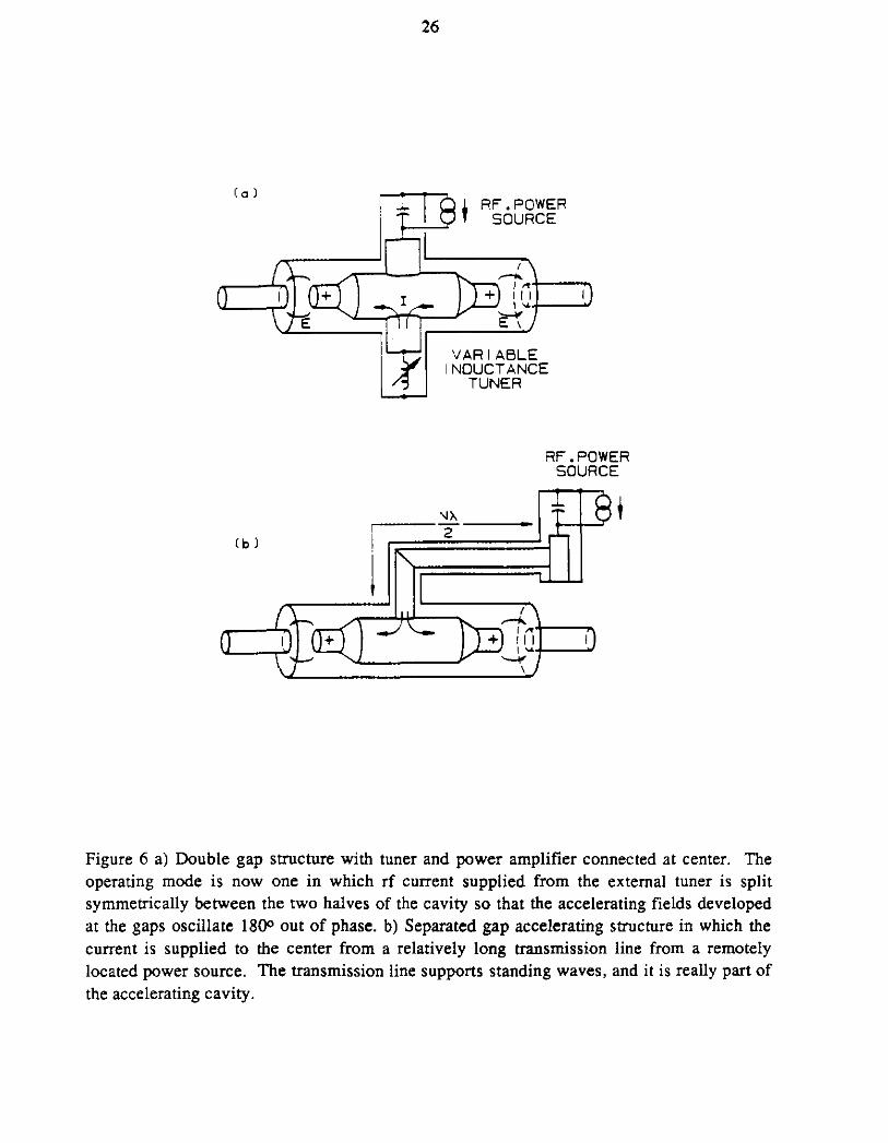
26

RF.POWER SOURCE

VARIABLE INDUCTANCE

TUNER

RF.POWER SOURCE

~--N>. __ ~-2

Figure 6 a) Double gap structure with tuner and power amplifier connected at center. The operating mode is now one in which rf current supplied from the external tuner is split symmetrically between the two ha! ves of the cavity so that the accelerating fields developed at the gaps oscillate 18{)0 out of phase. b) Separated gap accelerating structure in which the current is supplied to the center from a relatively long transmission line from a remotely located power source. The transmission line supports standing waves, and it is really part of the accelerating cavity.

27

roughly twice as much energy as in the tuned cavity example. Since the impedances of the two line sections are presented to the tuner in parallel, it must be capable of developing an inductive reactance lower by half than the previous example. voltage developed by this geometry is

V 2v . 2rcD

'cc = g sm--x-.

The maximum accelerating

( 45)

where D is the line half length. Maximum voltage is developed when D=A./4 and this may be achievable with an appropriately graded Re, but the result may not achieve as low an R/Q

value as desired.

The Q of such a cavity is calculable just as a ferrite tunable cavity. The shunt im­pedance presented to the beam, as compared to that measured in the laboratory, depends on the length. A current generator delivering resonant frequency current i to one of the gaps will develop a voltage v g at that gap. One can infer from this a resistance R = v gii at that gap,

and the power dissipated in the cavity (using peak values of voltage and current) is

• P

ivg ii'R VgVg =z =-2- = 2R. ( 46)

An additional current generator, at some other phase angle, applied to either gap, will de­velop an additional voltage at the new phase angle at each gap. The two voltages must be added vectorially and the power calculated using Eq. 46.

We again consider structures with half-length D = mA.14 (m < 1). Beam current entering the cavity from the left can be considered to excite the cavity at phase angle <I> = mrr/2 (with respect to <I>= 0 at cavity center plane). The same current, leaving the cavity at the right gap, excites the cavity with current of opposite sign delayed by -<I>. The beam generated cavity voltage is

2 .IR . re = J sm m2

The power delivered to the rf cavity by beam excitation is

(47)

( 48)

For beam loading, stability, and R/Q considerations, the shunt impedance of such a cavity

28

must be considered to be R5 = 4R sin2(mrr/2) where R is the shunt impedance inferred from

external measurement at one gap.

This geometry allows several ferrite tuners to be connected to the cavity in parallel at the mid-point so that they do not occupy space along the beam pipe, and they are easily accessible for cooling, application of tuning bias current, maintenance, etc. External place­ment of the tuning inductance establishes the center point of the cavity at voltage and im­pedance levels convenient for input power coupling. The wide range of beam loading and tuning impedance usually encountered do not establish this point as one of constant real load impedance suitable for termination of a long transmission line, however, it is usually a suitable point to couple to the anode of a large power amplifier tube located very close to the cavity.

The in-phase spearated gap cavity can be coupled through a long transmission line to a remotely located power amplifier when operated at fixed frequency. In such a case the transmission line will usually have standing waves and, in fact, becomes part of the resonant accelerating structure. This is the basis for the Fermillab TEVA TRON rf system. I 9

Mechanical Considerations

Accelerator rf cavities must operate reliably and stably for long periods in a remote, hostile, and, only occasionally accessible environment. To meet these requirements they should be built as simply and ruggedly as possible. The very high rf currents encountered at the low impedance regions of the cavity are capable of damaging loose or casually assembled joints and the very high electric fields at other points can result in damaging arcs or dielectric failure of vacuum seals. These hazards can be minimized by care and ingenuity in the selection and placement of rf clamp joints, dielectric and metallic materials, ferrites, etc. \1any unexpected malfunctions will be exposed through the development of a complete and operable prototype for each accelerating system. Frequently such prototypes evolve into spare systems which can be kept in operation outside of the accelerator, providing immediate access to a known reliable component in case of accelerator failure. Accelerator access time is extremely expensive time, and the cost of additional operating systems is easily offset by the reduction of true maintenance time they generate.

CONCLUSION

These notes are a collection of a few ideas developed over a number of years of engage­ment with a variety of proton accelerator rf systems. It is hoped that they may be useful to persons entering the field.

29

The author wishes to thank collectively all of the many people with whom he has collaborated or from whom he has assimilated or stolen ideas, with the sole purpose of making the best possible instruments for doing the best possible physics.

APPENDIX A Relativistic Mechanics

The charged particles (protons) under consideration here are acted upon by electric and magnetic fields in their motion around closed orbits in the accelerator. The force acting on the particles is the Lorenz force (MKs units)

F = e[v x B(s,t) + E(s,t)]

h ds A

were= v = -d t s

and s is the distance along the particle orbit. In a proton synchrotron the ideal orbit is a closed path of definite length, or circumference C. The path is usually not quite circular but one can define an average radius such that 2rrR = C.

The forces resulting from magnetic fields B are always perpendicular to the direction of motion, hence, they cannot affect the particle energy, but serve primarily to establish the path curvature required for a closed orbit. It is the electric fields E(s,t) provided by the rf system and directed along the path s which can affect the particle energy.

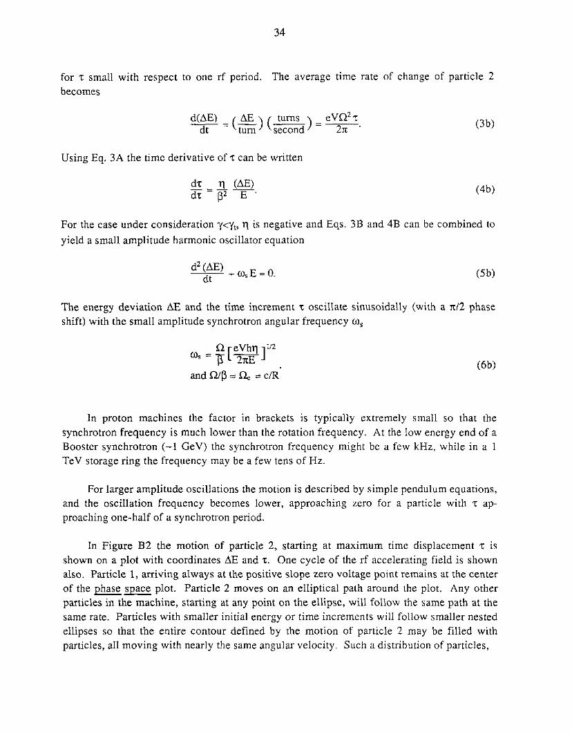
The particles under consideration are relativistic, i.e., their speeds are reasonably near the free space speed of light c. Since these speeds cannot exceed c, momentum changes resulting from the longitudinal fields E(s,b) result in changes in both particle speed and mass. Some useful relationships can be derived from the energy-momentum triangle shown in Figure Al.

If a particle energy is increased slightly by passage through an rf accelerating cavity electric field, the increase in particle momentum dp (or dp/p) is composed partially of an increase in speed d~/~ and partially an increase in mass. For a fixed average orbit bending magnetic field the two changes will have opposite effects on the period of time required for a particle to complete one orbital path. An increase in speed will, of course, shorten the period while an increase in mass will cause the particle to pass through the bending field with slightly larger average radius, increasing its path length and orbital period. In strong focuss­ing synchrotrons magnetic bending and focussing fields are composed so that changes in

30

RELATIVISTIC PROPERTIES OF PARTICLES

rKineti~ rRest Mass] Total Energy= lEnergyJ +LEnergy

Define J3 =vie c = vel. of light

free space

Energy Momentum Triangle

pc= J3E

dE_dY_r.t2~ E - y -p p [ ]

-112 Y= l-J32

~ = Cl3ri f = Cf-1) 1 dP dt = F = e[(VxB) + E]

For Proton

ITIQC2: 938.28 MeV

Figure Al) Some useful relationships between various kinematic properties of particles.

31

orbit length resulting from increases in momentum are reduced somewhat by a momentum compaction factor a.

de =CJ.~ c p

Also

The fractional change in rotation period can now be related to a change in momentum,

dT _ dC _ dV _ ( l_ _ l_ ) ~ _ ,, dp _ 21_ dE T - c v - ii i p - 'I p - ~2 E

(la)

(2a)

(3a)

The constant "'ft (transition gamma) is determined by the detailed design of the bending and

focussing magnets in the ring. 11, referred to as the revolution frequency dispersion or mixing factor, is a function of particle energy (or gamma). We see that at y = Yt a change in

momentum results in no change in rotational period (or frequency). For energies such that Y<Yt 11 is negative and the change in particle speed dominates, so an increase in energy results

in a decrease in rotation period (increase in rotational frequency), while for "'f>Yt the converse

is true.

These relationships between rotation period and momentum need not be related uniquely to changes in energy associated with the presence of rf longitudinal fields. They very generally relate the periods of particles of different momentum moving within the momentum acceptance or momentum aperture of the ring. Frequently the incremental energy ~ or momentum D,p are defined with respect to a particle on a central orbit or synchronous particle. Deviations from the arrival time or energy of a synchronous particle are most conveniently represented by pairs of variables which are cannonically conjugate in the sense of Hamiltonian mechanics. For this illustration we use two such variables, the energy devia­tion D,E and the arrival time increment 't. Other useful pairs of variables are momentum and path length (Ap) and (As), or W = AE/hn and Ll.'1J, the angle on the rf wave corresponding to the time increment 't.

An excellent review of Hamiltonian single particle dynamics may be found in Ref. 9.

APPENDIX B Synchrotron Motion

There are many excellent and detailed treatments of synchrotron motion m the literatureJl,2,3bJ We propose to develop here a simple and intuitive model for such motion

32

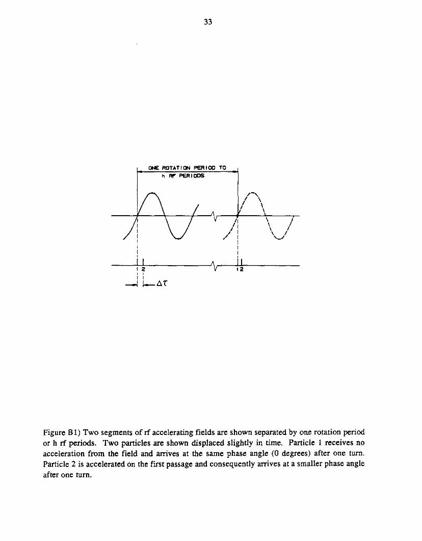
with only that mathematical detail necessary to motivate the design of rf accelerating cavities. We examine the motion of two particles and their interaction with an rf field as shown in Figure B 1. Initially each of the particles has the same energy and each requires a time T 0 the synchronous rotation period to make one complete orbit turn. The rf period is

shorter than T 0 by an integral factor h, the rf harmonic number. Particle 1 passes the ac­

celerating gap at a time when the accelerating voltage is zero so its momentum remains unchanged, consequently, after one turn (exactly h rf periods) it arrives at the accelerating gap when the voltage is again zero and the process continues with no change in particle 1 momentum. (We assume that this particle loses negligible energy to its environment during its orbital travel; true for protons at presently attainable energy, but not true for electrons.) Particle 2 arrives at the accelerating gap a few nanoseconds later than particle 1, and it experiences a non-zero accelerating field, increasing its momentum. Here we considered the velocity increase to be dominant, Y<Yt, Tl negative. Particle 2 traverses its orbit in a time

slightly less than T0, arrives slightly earlier, where it again receives an acceleration, and the

process continues, particle 2 moving toward particle 1 in time. When particle 2, arriving at successively earlier times, arrives coincident with particle 1, its momentum has been substan­tially increased so it continues to arrive at earlier times, now experiencing a repeated decelerating field, until it again reaches the synchronous momentum, now arriving earlier by the same time increment that it initially had for late arrivals. The particle now continues to be decelerated, arriving successively later and the process continues, with particle 2 execut­ing synchroton time or phase oscillation about the positive slope zero field point on the rf wave.

The rotational angular velocity of a hypothetical particle moving with velocity c (infinite energy) would be Qc = c/R and that of a finite energy particle characterized by P is

n = pnc.

The rf voltage developed at an accelerating gap by an rf system operating at harmonic number his

v(t) = V sin(hQt).

The change in energy, llE of a particle crossing the gap at time t during one turn will be

(tLlE) = e V sin (hilt) urn

: eV(h!lt)

(1 b)

(2b)

33

ONE ROTATION F'ERIOO TO n RI' F'ER I ODS

/1

'1 /1 / I

I I I

' '

,-, I \

I I I I

\ I \ I I I \ I ,_,,

~~~'~'~~~~~~~~----'-'~'~~~~-\ 2 v 12 ' ' I I

--I I-- ti. r

Figure B 1) Two segments of rf accelerating fields are shown separated by one rotation period or h rf periods. Two particles are shown displaced slightly in time. Particle 1 receives no acceleration from the field and arrives at the same phase angle (0 degrees) after one turn. Particle 2 is accelerated on the first passage and consequently arrives at a smaller phase angle after one tum.

34

for t small with respect to one rf period. The average time rate of change of particle 2 becomes

d(L'.E) = ( L'.E) ( turns ) = eVU2 t. dt tum second 2rr

Using Eq. 3A the time derivative oft can be written

dt Tl (6.E) dt = ~2 -r·

(3b)

(4b)

For the case under consideration Y<Yt> T] is negative and Eqs. 3B and 4B can be combined to

yield a small amplitude harmonic oscillator equation

d2 (L'.E) dt + WsE = 0. (5b)

The energy deviation 6.E and the time increment t oscillate sinusoidally (with a rr/2 phase shift) with the small amplitude synchrotron angular frequency w,

Q [eVhT] ]112 w, = 1l° 2rrE

and nip = Uc = c/R (6b)

In proton machines the factor in brackets is typically extremely small so that the synchrotron frequency is much lower than the rotation frequency. At the low energy end of a Booster synchrotron (-1 GeV) the synchrotron frequency might be a few kHz, while in a 1

Te V storage ring the frequency may be a few tens of Hz.

For larger amplitude oscillations the motion is described by simple pendulum equations, and the oscillation frequency becomes lower, approaching zero for a particle with t ap­proaching one-half of a synchrotron period.

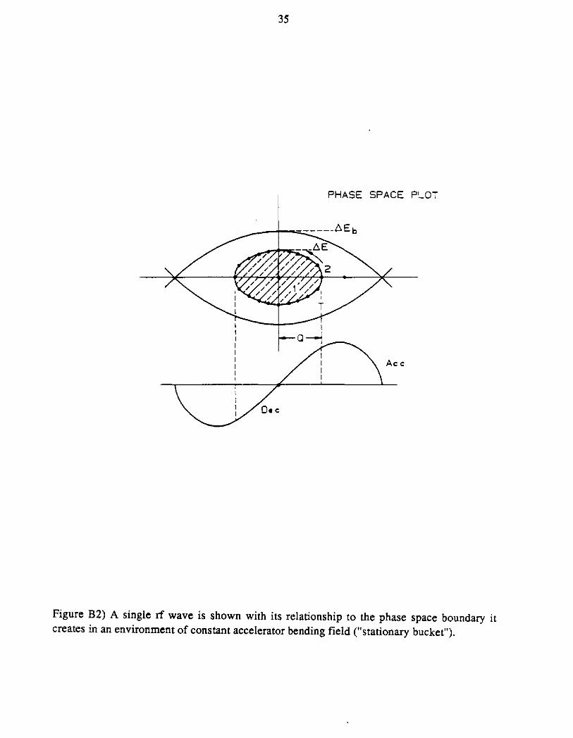
In Figure B2 the motion of particle 2, starting at maximum time displacement t is shown on a plot with coordinates L'.E and t. One cycle of the rf accelerating field is shown also. Particle l, arriving always at the positive slope zero voltage point remains at the center of the phase space plot. Particle 2 moves on an elliptical path around the plot. Any other particles in the machine, starting at any point on the ellipse, will follow the same path at the same rate. Particles with smaller initial energy or time increments will follow smaller nested ellipses so that the entire contour defined by the motion of particle 2 may be filled with particles, all moving with nearly the same angular velocity. Such a distribution of particles,

35

PHASE SPACE PLOT

Ace

Figure B2) A single rf wave is shown with its relationship to the phase space boundary it creates in an environment of constant accelerator bending field ("stationary bucket").

36

confined to a region ±'t on the rf curve, is a beam bunch. The ~ of the ellipse defined by the maximum amplitude particles is referred to as the longitudinal emittance of a single bunch.

S = itllli't e V-s. (7b)

Consider now a hypothetical particle which starts incrementally prior to the negative slope zero rf voltage point, i.e., 't = n/2 - 8. Such a particle would, at first, receive an ex­tremely small acceleration per tum, and it would move very slowly toward earlier time where the acceleration per tum becomes larger until it reaches a maximum at 't = it/4. Such a particle would oscillate very slowly over the entire rf period, generating the dashed path shown. It would receive the maximum possible acceleration and deceleration each cycle. The dashed curve represents a separatrix, and it defines the boundary of the rf system capa­bility for confining particles, commonly referred to as an rf bucket. Particles with variables within the separatrix will move on closed contours within the bucket while particles outside of the separatrix will move along paths outside of the series of buckets and are not confined by the rf system.

Some useful relationships are presented here without derivation.

[ 2E, V ]112

Bucket Height t.E0 = ~ 1th I '11 I eV

8Lllio Bucket Area A0 = hQ eV-s

It is convenient to define an angle <I> on the rf wave,

The energy deviation i'iE of a particle starting from angle <I> is

(Sb)

(9b)

(!Ob)

(11 b)

37

List of References I. K. Halbach and R. F. Heisinger, Part. Accelerators, 2 (1976) 213 2. T. Weiland, NIM 216 (1983) 329 and DESY-M-82-024, (1982)

3. T. Weiland, Part. Accelerators, 11 (1985) 4. G. Dome, Proc. 1976 Proton Linear Acee!. Conf., Chalk River, Ontario, Canada ( 1976)

138-147 5. W.R. Smythe, IEEE Trans. Nucl. Sci. NS-30, (1983) 2173 6. W.R. Smythe and T. G. Brophy, IEEE Trans. Nucl. Sci. NS-32, (1985) 2951 7. P. B. Wilson, AIP Conf. Proc. No. 87 (Physics of High Energy Acee!., Fermilab Summer

School), (1981) 452 8. R. Johnson, S. van der Meer, F. Pedersen, and G. Shering, IEEE Proc. Nucl. Sci, NS-30,

(1983) 2290 9. F. T. Cole, AIP Conf. Proc. 153 (Physics of Particle Accelerators, SLAC, 1985) 45

10. C. Bovet, R. Gouiran, I. Gumowski, R. Reich, CERN Report DL/70/4, (1970) Appendix D

11. J. Griffin, IEEE Proc. Nuc! Sci. NS-22, (1975) 1910 12. P. B. Wilson, Proc. IX Internat. Conf. on High Energy Accelerators, SLAC, (1974) 57 13. V. Vaccaro, Comments on Beam Instability, Eloisatron Workshop, Ettore Majorana

Center, (1987) 14. K. Robinson, Cambridge Electron Acee!. Lab Rep. 1010, (1964) 15. A. Hofmann, Proc. Internat. School of Particle Accelerators, Ettore Majorana Center,

(1977) 139 16. A. Hofmann, ibid. 17. E. Keil and W. Schnell, CERN Rep. ISR-TH-RF/69-48, (1969) 18. J.E. Griffin and Q. A. Kerns, IEEE Trans. Nucl. Sci. NS-18, (1971) 241 19. Q. Kerns et al., IEEE Trans. Nucl. Sci. NS-28, (1981) 2782