642 IEEE/ASME TRANSACTIONS ON MECHATRONICS, VOL. 19, NO. 2, APRIL 2014
A Validated Feasibility Prototype for AUVReconfigurable Magnetic Coupling Thruster
Olivier Chocron, Urbain Prieur, and Laurent Pino
Abstract—This paper presents the concept and design of a newreconfigurable magnetic-coupling thruster (RMCT). Mechanicalmodels, as well as digital and real-world experiments, are pro-posed to understand the fundamental aspects of such technology.The principle of RMCT is to reorient the propeller, and thereforethe thrust vector, to the desired direction without adding or mov-ing any motors. The focus of this study is to propose a new designto solve the problems raised in a previous work on RMCT and tounderstand how the transmitted coupling torque behaves with re-gard to the new kinematics of the propeller shaft. After introducingthe models underlying this thruster design, we build a numericalsimulation and validate it through experimental results. The per-formance of this design is then discussed based on open-loop trialsand its potential integration and control. The conclusion proposesguidelines for developing an underwater prototype that will bedesigned and tested on real autonomous underwater vehicles.
Index Terms—Actuators, magnetic devices, propulsion, under-water vehicle propulsion.
I. INTRODUCTION
UNDERWATER vehicles are used in ocean engineering [1]and military tasks [2], but the last few years have seen a
rapid development of their needs due to breakthroughs in thetechnology and energy sectors. The next step in offshore engi-neering is to design, build, and operate tidal and offshore windturbines. These activities will require new underwater vehiclesfor both construction and maintenance tasks [3]. Remotely op-erated vehicles (ROV) are widely deployed in the industry be-cause their use depends almost entirely on human understandingand decision making based on what the robot detects through itscameras or sonars (oil, telecommunications, or defence sectors).It has become clear in recent offshore oil pumping history thatreadily available, flexible, and efficient deep-water interven-tion robots are dearly needed. Due to hostile environments,strong currents, and nearby dangers such as gas/fluid ejection orcomplex underwater structures, the underwater robots requireextensive maneuvering capabilities and autonomy. At the sametime, the domain of autonomous underwater vehicles (AUV) cannow make use of research in mobile robotics such as advancedcontrol [4] [5] or visual/acoustic servoing [6]. These advances,
Manuscript received February 6, 2012; revised July 11, 2012 and December3, 2012; accepted January 14, 2013. Date of publication April 1, 2013; date ofcurrent version February 20, 2014. Recommended by Technical Editor Y. Sun.
O. Chocron and L. Pino are with the Laboratoire Brestois de Mecanique et desSystemes, Ecole Nationale d’Ingenieurs de Brest, UEB, Technopole de BrestIroise, 29238 Brest Cedex 3, France (e-mail: [email protected]; [email protected]).
U. Prieur is with the Institut des Systemes Intelligents et de Robotique, Univer-site Pierre et Marie Curie, 75005 Paris, France (e-mail: [email protected]).
Color versions of one or more of the figures in this paper are available onlineat http://ieeexplore.ieee.org.
Digital Object Identifier 10.1109/TMECH.2013.2250987
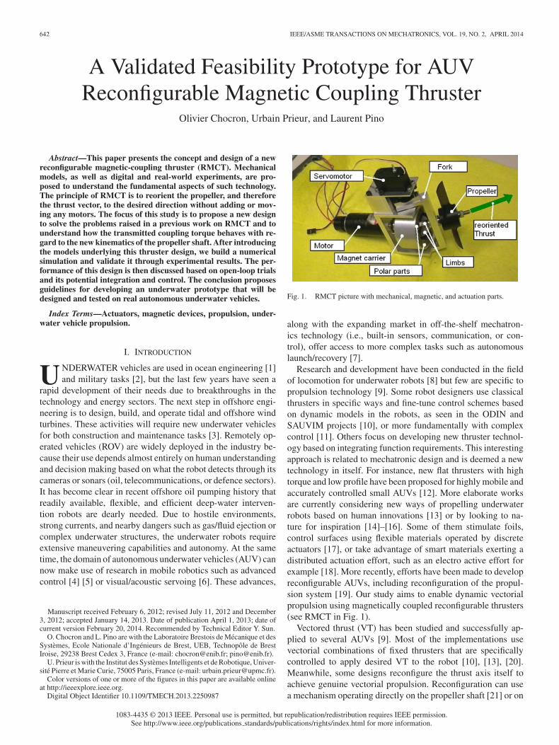
Fig. 1. RMCT picture with mechanical, magnetic, and actuation parts.
along with the expanding market in off-the-shelf mechatron-ics technology (i.e., built-in sensors, communication, or con-trol), offer access to more complex tasks such as autonomouslaunch/recovery [7].
Research and development have been conducted in the fieldof locomotion for underwater robots [8] but few are specific topropulsion technology [9]. Some robot designers use classicalthrusters in specific ways and fine-tune control schemes basedon dynamic models in the robots, as seen in the ODIN andSAUVIM projects [10], or more fundamentally with complexcontrol [11]. Others focus on developing new thruster technol-ogy based on integrating function requirements. This interestingapproach is related to mechatronic design and is deemed a newtechnology in itself. For instance, new flat thrusters with hightorque and low profile have been proposed for highly mobile andaccurately controlled small AUVs [12]. More elaborate worksare currently considering new ways of propelling underwaterrobots based on human innovations [13] or by looking to na-ture for inspiration [14]–[16]. Some of them stimulate foils,control surfaces using flexible materials operated by discreteactuators [17], or take advantage of smart materials exerting adistributed actuation effort, such as an electro active effort forexample [18]. More recently, efforts have been made to developreconfigurable AUVs, including reconfiguration of the propul-sion system [19]. Our study aims to enable dynamic vectorialpropulsion using magnetically coupled reconfigurable thrusters(see RMCT in Fig. 1).
Vectored thrust (VT) has been studied and successfully ap-plied to several AUVs [9]. Most of the implementations usevectorial combinations of fixed thrusters that are specificallycontrolled to apply desired VT to the robot [10], [13], [20].Meanwhile, some designs reconfigure the thrust axis itself toachieve genuine vectorial propulsion. Reconfiguration can usea mechanism operating directly on the propeller shaft [21] or on
CHOCRON et al.: VALIDATED FEASIBILITY PROTOTYPE FOR AUV RECONFIGURABLE MAGNETIC COUPLING THRUSTER 643
the propeller duct that orients the water flow [22] (Bluefin), or itcan be achieved using water jets [23]. Magnetic coupling (MC)is already used in underwater robotics for manipulators [24]or thrusters [20]. The concept has been applied to ROVs since1975 [25] and continues to be developed according to mod-ern electromechanical devices such as brushless motors [26].The principle is to make the coupling between the driving anddriven rotors immaterial, i.e., without a mechanical link. This isusually done by using magnets on both rotor sides to create amagnetic loop linking motor and propeller shaft rotations. Thistechnology was first introduced for applications at great depthsbecause it was a good way to avoid the leaks that tend to occurwith sealed rotating shafts (instead of using oil-filled motors).Another advantage is that the technology is intrinsically a torquelimiter that can save the thruster electromechanics (the couplingwill disconnect in the case of a severe rupture of the load torque:if entangled in a cable for instance). This uncoupling can also bediagnosed through voltage and/or current monitoring and trig-ger abort or survival modes. Finally, the greatest advantage isthat MCs can turn in any direction without losing their cohe-sive force (and even reinforcing it in some conditions) or theirfundamental property of synchronous drive. It is precisely thisvaluable feature that we rely on when we propose the conceptof the reconfigurable magnetic-coupling thruster (RMCT). Ourstudy means to exploit the advantages of MC in order to pro-pose a new enabling technology for VT. RMCT has alreadybeen studied to assess its potential [27], [28]. We here proposeto study an innovative RMCT design which we have developedup to the stage of a feasibility prototype (see Fig. 1). A 3-DRMCT prototype design is proposed and detailed in Section II,while magnetomechanical models are developed in Section III.The key parameters are identified through real-world experi-ments in Section IV and used to validate a numerical simulationin Section V. To end this paper, we present a general conclusionwhich includes expectations, limits, and future evolutions of thisinnovative technology.
II. DESCRIPTION OF THE RMCT
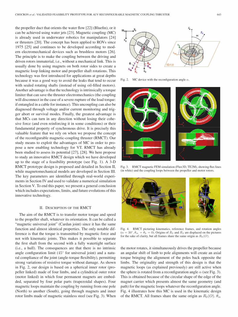
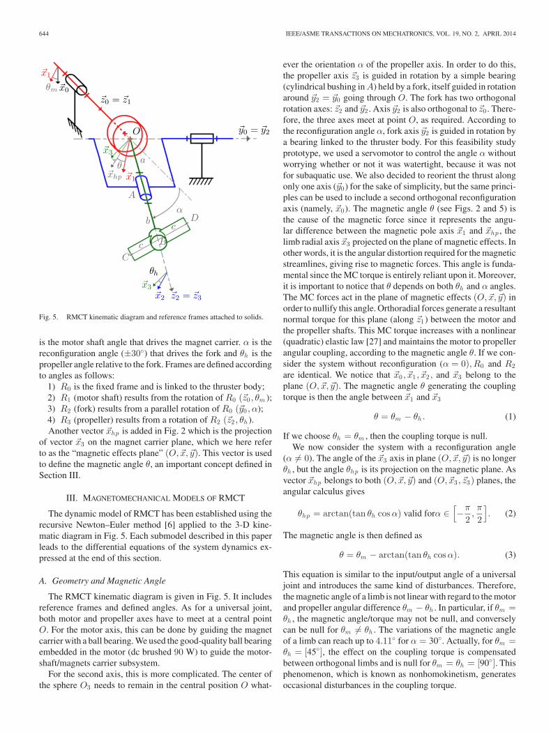
The aim of the RMCT is to transfer motor torque and speedto the propeller shaft, whatever its orientation. It can be called a“magnetic universal joint” (Cardan joint) since it has the samefunction and almost identical properties. The only notable dif-ference is that the torque is transmitted by magnetic force andnot with kinematic joints. This makes it possible to separatethe first shaft from the second with a fully watertight surface(i.e., a hull). The consequences are that there is no intrinsicangle configuration limit (45◦ for universal joint) and a natu-ral compliance of the joint (angle-torque flexibility), permittingstrong variations of resistive torque without damage. As shownin Fig. 2, our design is based on a spherical inner rotor (pro-peller linked) made of four limbs, and a cylindrical outer rotor(motor linked) in which four permanent magnets are embed-ded, separated by four polar parts (trapezoidal shapes). Fourmagnetic loops maintain the coupling by running from one pole(North) to another (South), going through magnets and innerrotor limbs made of magnetic stainless steel (see Fig. 3). When
Fig. 2. MC device with the reconfiguration angle α.
Fig. 3. RMCT magnetic FEM simulation (Flux3D, TE2M), showing flux lines(in white) and the coupling loops between the propeller and motor rotors.
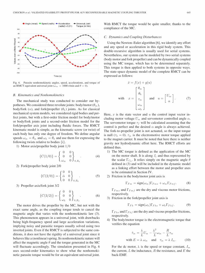
Fig. 4. RMCT picturing kinematics, reference frames, and rotation angles(α = 30◦, θm = θh = 0). Origins of R2 and R3 are displaced on the picturesfor the sake of clarity, but all frames share the same origin as R0 (O).
the motor rotates, it simultaneously drives the propeller becausean angular shift of limb to pole alignments will create an axialtorque bringing the alignment of the poles back opposite thelimbs. The originality and strength of this design is that themagnetic loops (as explained previously) are still active whenthe sphere is rotated from a reconfiguration angle α (see Fig. 3).This is obtained because of the circular shape of the edge of themagnet carrier which presents almost the same geometry (andpath) for the magnetic loops whatever the reconfiguration angle.Fig. 4 illustrates how this MC is used in the kinematic designof the RMCT. All frames share the same origin as R0(O). θm
644 IEEE/ASME TRANSACTIONS ON MECHATRONICS, VOL. 19, NO. 2, APRIL 2014
Fig. 5. RMCT kinematic diagram and reference frames attached to solids.
is the motor shaft angle that drives the magnet carrier. α is thereconfiguration angle (±30◦) that drives the fork and θh is thepropeller angle relative to the fork. Frames are defined accordingto angles as follows:
1) R0 is the fixed frame and is linked to the thruster body;2) R1 (motor shaft) results from the rotation of R0 (�z0 , θm );3) R2 (fork) results from a parallel rotation of R0 (�y0 , α);4) R3 (propeller) results from a rotation of R2 (�z2 , θh ).Another vector �xhp is added in Fig. 2 which is the projection
of vector �x3 on the magnet carrier plane, which we here referto as the “magnetic effects plane” (O, �x, �y). This vector is usedto define the magnetic angle θ, an important concept defined inSection III.
III. MAGNETOMECHANICAL MODELS OF RMCT
The dynamic model of RMCT has been established using therecursive Newton–Euler method [6] applied to the 3-D kine-matic diagram in Fig. 5. Each submodel described in this paperleads to the differential equations of the system dynamics ex-pressed at the end of this section.
A. Geometry and Magnetic Angle
The RMCT kinematic diagram is given in Fig. 5. It includesreference frames and defined angles. As for a universal joint,both motor and propeller axes have to meet at a central pointO. For the motor axis, this can be done by guiding the magnetcarrier with a ball bearing. We used the good-quality ball bearingembedded in the motor (dc brushed 90 W) to guide the motor-shaft/magnets carrier subsystem.
For the second axis, this is more complicated. The center ofthe sphere O3 needs to remain in the central position O what-
ever the orientation α of the propeller axis. In order to do this,the propeller axis �z3 is guided in rotation by a simple bearing(cylindrical bushing in A) held by a fork, itself guided in rotationaround �y2 = �y0 going through O. The fork has two orthogonalrotation axes: �z2 and �y2 . Axis �y2 is also orthogonal to �z0 . There-fore, the three axes meet at point O, as required. According tothe reconfiguration angle α, fork axis �y2 is guided in rotation bya bearing linked to the thruster body. For this feasibility studyprototype, we used a servomotor to control the angle α withoutworrying whether or not it was watertight, because it was notfor subaquatic use. We also decided to reorient the thrust alongonly one axis (�y0) for the sake of simplicity, but the same princi-ples can be used to include a second orthogonal reconfigurationaxis (namely, �x0). The magnetic angle θ (see Figs. 2 and 5) isthe cause of the magnetic force since it represents the angu-lar difference between the magnetic pole axis �x1 and �xhp , thelimb radial axis �x3 projected on the plane of magnetic effects. Inother words, it is the angular distortion required for the magneticstreamlines, giving rise to magnetic forces. This angle is funda-mental since the MC torque is entirely reliant upon it. Moreover,it is important to notice that θ depends on both θh and α angles.The MC forces act in the plane of magnetic effects (O, �x, �y) inorder to nullify this angle. Orthoradial forces generate a resultantnormal torque for this plane (along �z1) between the motor andthe propeller shafts. This MC torque increases with a nonlinear(quadratic) elastic law [27] and maintains the motor to propellerangular coupling, according to the magnetic angle θ. If we con-sider the system without reconfiguration (α = 0), R0 and R2are identical. We notice that �x0 , �x1 , �x2 , and �x3 belong to theplane (O, �x, �y). The magnetic angle θ generating the couplingtorque is then the angle between �x1 and �x3
θ = θm − θh . (1)
If we choose θh = θm , then the coupling torque is null.We now consider the system with a reconfiguration angle
(α �= 0). The angle of the �x3 axis in plane (O, �x, �y) is no longerθh , but the angle θhp is its projection on the magnetic plane. Asvector �xhp belongs to both (O, �x, �y) and (O, �x3 , �z3) planes, theangular calculus gives
θhp = arctan(tan θh cos α) valid forα ∈[−π
2,π
2
]. (2)
The magnetic angle is then defined as
θ = θm − arctan(tan θh cos α). (3)
This equation is similar to the input/output angle of a universaljoint and introduces the same kind of disturbances. Therefore,the magnetic angle of a limb is not linear with regard to the motorand propeller angular difference θm − θh . In particular, if θm =θh , the magnetic angle/torque may not be null, and converselycan be null for θm �= θh . The variations of the magnetic angleof a limb can reach up to 4.11◦ for α = 30◦. Actually, for θm =θh = [45◦], the effect on the coupling torque is compensatedbetween orthogonal limbs and is null for θm = θh = [90◦]. Thisphenomenon, which is known as nonhomokinetism, generatesoccasional disturbances in the coupling torque.
CHOCRON et al.: VALIDATED FEASIBILITY PROTOTYPE FOR AUV RECONFIGURABLE MAGNETIC COUPLING THRUSTER 645
Fig. 6. Parasite nonhomokinetic angles, speed, accelerations, and torque ofan RMCT equivalent universal joint (ωm = 1000 r/min and θ = 0).
B. Kinematics and Nonhomokinetics
The mechanical study was conducted to consider our hy-potheses. We considered three revolute joints: body/motor (θm ),body/fork (α), and fork/propeller (θh ) joints. As for classicalmechanical system models, we considered rigid bodies and per-fect joints, but with a first-order friction model for body/motoror body/fork joints and a second-order friction model for thefork/propeller axis joint including fluidic forces. The RMCTkinematic model is simple, as the kinematic screw (or twist) ofeach body has only one degree of freedom. We define angularspeeds ωm = θm and ωh = θh and use them for expressing thefollowing twists relative to bodies {i}.
1) Motor axis/propeller body joint 1/0
{C(1/0)} =
{ 0 00 0
ωm 0
}
0,R0
. (4)
2) Fork/propeller body joint 2/0
{C(2/0)} =
{ 0 0α 00 0
}
0,R0
. (5)
3) Propeller axis/fork joint 3/2
{C(3/2)} =
{ 0 00 0ωh 0
}
0,R2
. (6)
The motor drives the propeller by the MC, but not with theexact same angle, as the coupling torque tends to cancel themagnetic angle that varies with the nonhomokinetic law (3).This phenomenon appears in a universal joint, with drawbacksbeing high-frequency speed and large acceleration variations,implying noisy and parasitic torques usually solved using twoinverted joints. Even if the RMCT is subjected to the same con-ditions, it does not have the rigidity of a universal joint since itbehaves like a (nonlinear) spring. Its nonhomokinetic nature willaffect the magnetic angle θ and the torque generated in the MCwill fluctuate accordingly. The simulation presented in Fig. 6uses second-order kinematics to show what the nonhomoki-netic parasite torque would be for an equivalent universal joint.
With RMCT the torque would be quite smaller, thanks to thecompliance of the MC.
C. Dynamics and Coupling Disturbances
Using the Newton–Euler algorithm [6], we identify any effortand any speed or acceleration in this rigid body system. Thisdouble-recursive algorithm is usually used for serial systems.Nevertheless, our system can be modeled by two serial systems(body motor and fork propeller) and can be dynamically coupledusing the MC torque, which has to be determined separately.This torque is then applied to both systems in opposite ways.The state-space dynamic model of the complete RMCT can beexpressed as follows:
x = f(x) + g(u)
with x =
⎡⎢⎢⎢⎢⎢⎣
θm
θh
τm
ωm
ωh
⎤⎥⎥⎥⎥⎥⎦
and u =[
Um
α
]. (7)
Here, x is the state vector and u the control input vector in-cluding motor voltage Um and servomotor controlled angle α.The servomotor torque τf will be calculated assuming that thecontrol is perfect and the desired α angle is always achieved.The fork-to-propeller joint is not actuated, so the input torqueis null (τh = 0). τm is the electromotive motor torque appliedto the magnet carrier. It must be noted that here there is neithergravity nor hydrodynamic effort here. The RMCT efforts aredefined thus.
1) The MC torque is defined as the application of the MCon the motor shaft. It is along �z1 and thus represented bythe scalar ΓC0 . It relies simply on the magnetic angle θdefined in (3) and will be included in the dynamic modelas a linking effort between the motor and propeller axesto be estimated in Section IV.
2) Friction in the body/motor joint axis is
ΓF m = sign(ωm )ΓF ms + ωm ΓF mf . (8)
ΓF ms and ΓF mf are the dry and viscous motor frictions,respectively.
3) Friction in the fork/propeller joint axis is
ΓF h = sign(ωh)ΓF hs + ωhΓF hf . (9)
ΓF hs and ΓF hf are the dry and viscous propeller frictions,respectively.
4) The body/motor torque is the electromagnetic torque thatverifies the equation
τm =λ
LUm − λ2
Lωm − R
Lτm
with E = λ ωm and τm = λ Im . (10)
For the dc motor, λ is the speed or torque constant, Im
the current, L the inductance, R the resistance, and E theback-EMF.
646 IEEE/ASME TRANSACTIONS ON MECHATRONICS, VOL. 19, NO. 2, APRIL 2014
5) The torque in the body/fork joint is applied by the servo-motor to control the angle α. It is only required in order tocheck its compatibility with our servomotor capabilities
τf = αIy23 + αωh(Ix3 − Iz3) + ΓF f . (11)
Iy23 is the combined moment of inertia of the fork andthe propeller on axis �y2 = �y0 , while Ix3 and Iz3 are themain moments of inertia for the only propeller (in R3).The Newton–Euler method gives the dynamic equations.
6) The motor shaft/magnet carrier S1 in R0
τm = Iz1 ωm − ΓC0 + ΓF m . (12)
Iz1 is the S1 main moment of inertia around �z1 = �z0 .7) The propeller shaft (considered symmetrical) S3 in R2
τh = 0 = Iz3 ωh + ΓC0 cos(α) + ΓF h . (13)
Iz3 is S3 main moment of inertia around �z3 = �z2 .Therefore, the reduced state-space system equations are
θm = ωm
θh = ωh
τm =λ
LUm − λ2
Lωm − R
Lτm
ωm =1
Iz1
(τm + ΓC0 − ΓF m )
ωh =1
Iz3
(−ΓC0 cos(α) − ΓF h). (14)
ΓC0 is dependent on θ, which is expressed according to statevariables in (3). We notice that α interferes directly (not onlyin ΓC0 ) with the propeller equation in the factor cos(α). Thisprevents us from going too far in the reconfiguration angle as itnullifies the driving torque for α = 90◦. It is for this reason thatwe kept our prototype under 30◦. An important result of thismodel is that the gyroscopic effect of coupled angular speedsωh and α plays a direct role for the servomotor torque alone.However, it will be applied to the revolute joint bearing (along�x2) generating a greater radial load on the bushing, and thusmore friction. This disturbance will be studied and identified inthe next section.
IV. IDENTIFICATION AND NUMERICAL SIMULATION
The RMCT model described in Section III requires the MCtorque equation presented in Section IV-A and its experimentalvalidation proposed in Sections IV-B and IV-C.
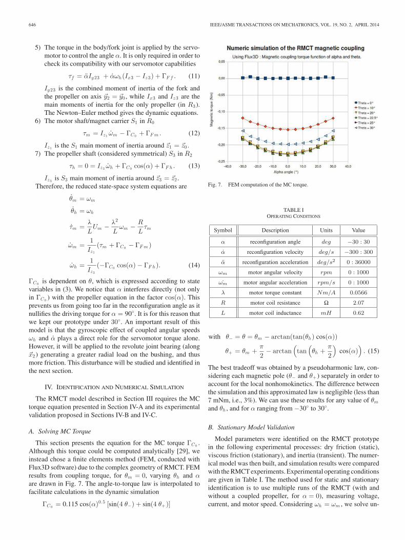
A. Solving MC Torque
This section presents the equation for the MC torque ΓC0 .Although this torque could be computed analytically [29], weinstead chose a finite elements method (FEM, conducted withFlux3D software) due to the complex geometry of RMCT. FEMresults from coupling torque, for θm = 0, varying θh and αare drawn in Fig. 7. The angle-to-torque law is interpolated tofacilitate calculations in the dynamic simulation
ΓC0 = 0.115 cos(α)0.5 [sin(4 θ−) + sin(4 θ+)]
Fig. 7. FEM computation of the MC torque.
TABLE IOPERATING CONDITIONS
with θ− = θ = θm − arctan(tan(θh) cos(α))
θ+ = θm +π
2− arctan
(tan
(θh +
π
2
)cos(α)
). (15)
The best tradeoff was obtained by a pseudoharmonic law, con-sidering each magnetic pole (θ− and θ+ ) separately in order toaccount for the local nonhomokinetics. The difference betweenthe simulation and this approximated law is negligible (less than7 mNm, i.e., 3%). We can use these results for any value of θm
and θh , and for α ranging from −30◦ to 30◦.
B. Stationary Model Validation
Model parameters were identified on the RMCT prototypein the following experimental processes: dry friction (static),viscous friction (stationary), and inertia (transient). The numer-ical model was then built, and simulation results were comparedwith the RMCT experiments. Experimental operating conditionsare given in Table I. The method used for static and stationaryidentification is to use multiple runs of the RMCT (with andwithout a coupled propeller, for α = 0), measuring voltage,current, and motor speed. Considering ωh = ωm , we solve un-
CHOCRON et al.: VALIDATED FEASIBILITY PROTOTYPE FOR AUV RECONFIGURABLE MAGNETIC COUPLING THRUSTER 647
Fig. 8. Model validation (α = 0) with angular speed ωm .
Fig. 9. Model validation (α = 0) with motor current Im .
known parameters according to stationary state-space equations(14)
without coupling
ΓF m = τm ⇒ ΓF ms + ωm ΓF mf = λIm (16)
with coupling
ΓF hs + ΓF ms + ωm (ΓF hf + ΓF mf ) = λIm . (17)
We can compare the real RMCT and the numerical model bylooking at stationary speed (see Fig. 8) or current (see Fig. 9)responses to a given voltage. The model is satisfactory for non-reconfigured RMCT and not so good for high reconfigurationangles (errors around 7%). This can be explained by the extrafriction load on the bushing which occurs when α �= 0. Identi-fied friction parameters are given in Table II.
TABLE IIFRICTION PARAMETERS FOR RMCT
Fig. 10. Comparison of step responses for real and simulated RMCT with α =0, Um = 6.44V, Im ∞ = 575 mA, ωm ∞ = 885 r/min, and τ0 = 350 ms.
TABLE IIIINERTIAL PARAMETERS FOR RMCT IN O
C. Dynamic Model Validation
For inertia identification, we use the step response (seeFig. 10), which yields the time constant τ0 (or 95% settlingtime T0). If the simulated times are higher than the experimen-tal ones, we lower simulation inertia parameters conversely. Thisis done first for uncoupled motor inertia to yield Iz1 , and thenfor whole RMCT, in order to obtain the propeller inertia Iz3 bysubtraction. The curve utilized is in fact the average of ten dif-ferent experimental trials under the same conditions. The inertiaand time parameters obtained by identification for a diverse setof step responses are given in Table III.
V. EXPERIMENTAL RESULTS AND PERFORMANCES
The experimental setup of the RMCT is shown in Fig. 1,along with the electronics conducting the power supply, PWMcontrol, and an analogical to digital converter (10 bits). Theservomotor is a Futaba S3003 powered with 6V. The electron-ics are controlled with a microrobotics device (dual-POB from
648 IEEE/ASME TRANSACTIONS ON MECHATRONICS, VOL. 19, NO. 2, APRIL 2014
POB-Technology1) enabling 20 Hz sampling and involving aWindows/PC serial link (see Section V-B).
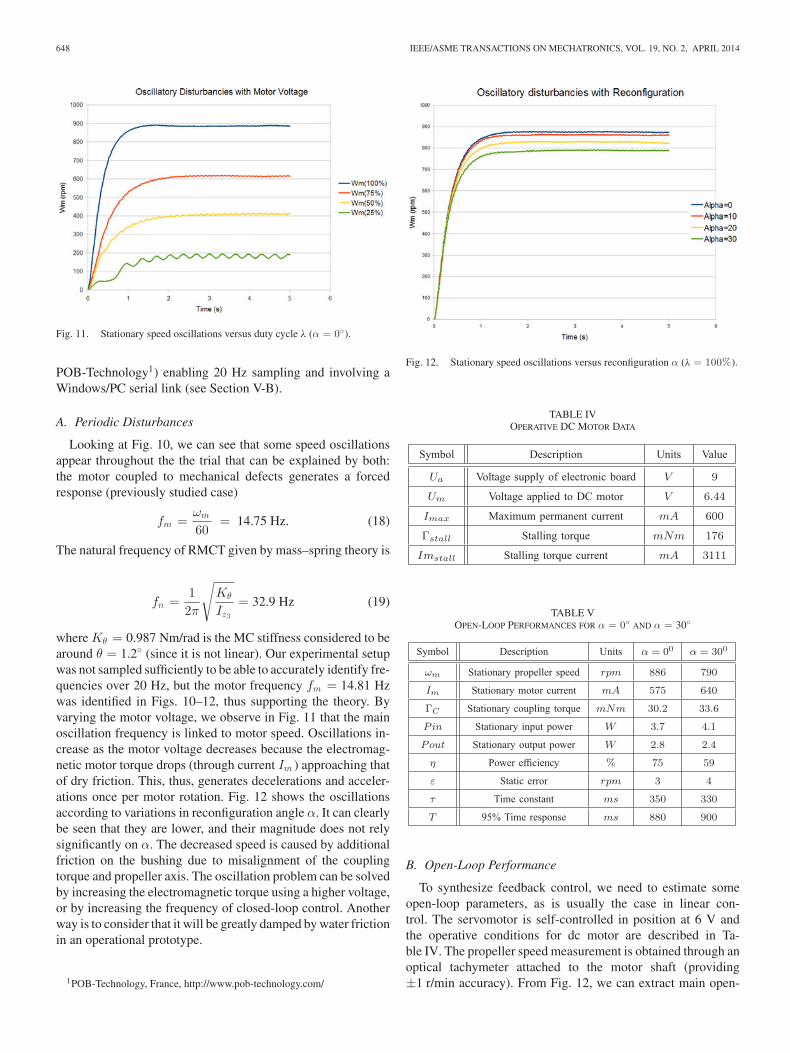
A. Periodic Disturbances
Looking at Fig. 10, we can see that some speed oscillationsappear throughout the the trial that can be explained by both:the motor coupled to mechanical defects generates a forcedresponse (previously studied case)
fm =ωm
60= 14.75 Hz. (18)
The natural frequency of RMCT given by mass–spring theory is
fn =12π
√Kθ
Iz3
= 32.9 Hz (19)
where Kθ = 0.987 Nm/rad is the MC stiffness considered to bearound θ = 1.2◦ (since it is not linear). Our experimental setupwas not sampled sufficiently to be able to accurately identify fre-quencies over 20 Hz, but the motor frequency fm = 14.81 Hzwas identified in Figs. 10–12, thus supporting the theory. Byvarying the motor voltage, we observe in Fig. 11 that the mainoscillation frequency is linked to motor speed. Oscillations in-crease as the motor voltage decreases because the electromag-netic motor torque drops (through current Im ) approaching thatof dry friction. This, thus, generates decelerations and acceler-ations once per motor rotation. Fig. 12 shows the oscillationsaccording to variations in reconfiguration angle α. It can clearlybe seen that they are lower, and their magnitude does not relysignificantly on α. The decreased speed is caused by additionalfriction on the bushing due to misalignment of the couplingtorque and propeller axis. The oscillation problem can be solvedby increasing the electromagnetic torque using a higher voltage,or by increasing the frequency of closed-loop control. Anotherway is to consider that it will be greatly damped by water frictionin an operational prototype.
1POB-Technology, France, http://www.pob-technology.com/
TABLE VOPEN-LOOP PERFORMANCES FOR α = 0◦ AND α = 30◦
B. Open-Loop Performance
To synthesize feedback control, we need to estimate someopen-loop parameters, as is usually the case in linear con-trol. The servomotor is self-controlled in position at 6 V andthe operative conditions for dc motor are described in Ta-ble IV. The propeller speed measurement is obtained through anoptical tachymeter attached to the motor shaft (providing±1 r/min accuracy). From Fig. 12, we can extract main open-
CHOCRON et al.: VALIDATED FEASIBILITY PROTOTYPE FOR AUV RECONFIGURABLE MAGNETIC COUPLING THRUSTER 649
loop performances for neutral (α = 0◦) and maximum (α =30◦) reconfigurations presented in Table V.
To be useful, such a device must allow for rapid reorientationof propeller direction, without losing thrust control. Table Vresults show that even for a 30◦ reconfiguration, little speedis lost (about 100 r/min). This perturbation, due to gyroscopiceffects, can easily be eliminated using linear control.
VI. CONCLUSION AND FUTURE WORK
These results are a good start considering that an electronicboard with very low control efficiency was used here (6 V/2 Aand 20 Hz sampling). The thrust effect on the AUV depends onits inertia and geometry, but it is obvious that changing thrustdirection using reconfiguration is much more efficient than vary-ing the speed of fixed thrusters [30]. The main reason is that tochange the thrust torque (for instance around the Yaw axis)with fixed thrusters, one needs to accelerate/decelerate the pro-pellers from positive to negative full speed (pulling or pushingwater), which takes much more time than simply rotating thepropellers. Future work (already in progress) will strive to de-sign an underwater prototype able to apply vectorial controlledthrust underwater. In order for this to work effectively, the tech-nical problem of actuating the reconfiguration angle remains tobe solved. The benefits of model-based control synthesis havebeen demonstrated by several works in recent years [31], thoughin the case of underwater vehicles, the task is not easy due toadded mass and hydrodynamic effects on AUVs [32]. We con-duct dynamical AUV modeling and simulation to develop, test,and validate future nonlinear model-based control laws.
ACKNOWLEDGMENT
The authors would like to thank their industrial partner,TE2M.2 Its expertise in MC has been a key asset for the RMCT.
REFERENCES
[1] V. Rigaud, “Innovation and operation with robotized underwater systems,”J. Field Robot., vol. 24, no. 6, pp. 449–459, Jul. 2007.
[2] G. Mailfert and J. Lemaire, “Redermor: An experimental platform forROV/AUV field sea trials,” in Proc. MTS/IEEE OCEANS Conf. Exhib.,Nice, France, Sep. 1998, vol. 1, pp. 357–362.
[3] S. Benelghali, M. Benbouzid, J. F. Charpentier, T. Ahmed-Ali, andI. Munteanu, “Experimental validation of a marine current turbine sim-ulator: Application to a permanent magnet synchronous generator-basedsystem second-order sliding mode control,” IEEE Trans. Ind. Electron.,vol. 58, no. 1, pp. 119–126, Jan. 2011.
[4] P. Hamelin, P. Bigras, J. Beaudry, P.-L. Richard, and M. Blain, “Discrete-time state feedback with velocity estimation using a dual observer: Appli-cation to an underwater direct-drive grinding robot,” IEEE/ASME Trans.Mechatronics, vol. 17, no. 1, pp. 187–191, Feb. 2012.
[5] D. Dong, C. Chen, J. Chu, and T.-J. Tarn, “Robust quantum-inspiredreinforcement learning for robot navigation,” IEEE/ASME Trans. Mecha-tronics, vol. 17, no. 1, pp. 86–97, Feb. 2012.
[6] Siciliano, K. Editors, Handbook of Robotics. Heidelberg, Germany:Springer-Verlag, 2008.
[7] A. J. Plueddemann, A. L. Kukulya, R. Stokey, and L. Freitag, “Au-tonomous underwater vehicle operations beneath coastal sea ice,”IEEE/ASME Trans. Mechatronics, vol. 17, no. 1, pp. 54–64, Feb. 2012.
[8] J. Yuh, “Design and control of autonomous underwater robots: A survey,”Autnom. Robot., vol. 8, no. 1, pp. 7–24, 2000.
2Techniques et Materiels Magnetiques, GTID Group, Brest, France
[9] A. R. Palmer, “Analysis of the propulsion and manoeuvring character-istics of survey-style AUVs and the development of a multi-purposeAUV,” Ph.D. dissertation, School Eng. Sci., Faculty Eng., Sci. Math.,Univ. Southampton, Southampton, U.K., 2009.
[10] A. Hanai, K. Rosa, S. Choi, and J. Yuh, “Experimental analysis andimplementation of redundant thrusters for underwater robots,” in Proc.IEEE/RSJ Int. Conf. Intell. Robot. Syst., Sendai, Japan, Sep. 2004,pp. 1109–1114.
[11] N. Leonard, “Periodic forcing, dynamics and control of underactuatedspacecraftand underwater vehicles,” in Proc. 34th IEEE Conf. Decis.Contr., New Orleans, LA, USA, Dec. 1995, vol. 4, pp. 3980–3985.
[12] M. Dunbabin, J. Roberts, K. Usher, G. Winstanley, and P. Corke, “Ahybrid AUV design for shallow water reef navigation,” in Proc. IEEE Int.Conf. Robot. Autom., Barcelona, Spain, Apr. 2005, pp. 2105–2110.
[13] I. Vasilescu, P. Varshavskaya, K. Kotay, and D. Rus, “Autonomous mod-ular optical underwater robot (amour) design, prototype and feasibilitystudy,” in Proc. IEEE Int. Conf. Robot. Autom., Barcelona, Spain, Apr.2005, pp. 1603–1609.
[14] G. Dogangil, E. Ozcicek, and A. Kuzucu, “Modeling, simulation, anddevelopment of a robotic dolphin prototype,” in Proc. IEEE Int. Conf.Mechatron. Autom., vol. 2, Niagara Falls, ON, Canada, Jul. 2005, pp. 952–957.
[15] C. Watts, E. McGookin, and M. Macauley, “Biomimetic propulsion sys-tems for mini-autonomous underwater vehicles,” in Proc. MTS/IEEEOCEANS Conf. Exhib., 2007, pp. 1–5.
[16] C. Zhou and K. H. Low, “Design and locomotion control of a biomimeticunderwater vehicle with fin propulsion,” IEEE/ASME Trans. Mechatron-ics, vol. 17, no. 1, pp. 25–35, Feb. 2012.
[17] K. Harper, M. Berkemeier, and S. Grace, “Modeling the dynamics ofspring-driven oscillating-foil propulsion,” IEEE J. Ocean. Eng., vol. 23,no. 3, pp. 285–296, Jul. 1998.
[18] M. Mojarrad, “AUV biomimetic propulsion,” in Proc. MTS/IEEEOCEANS Conf. Exhib., Providence, RI, USA, Sep. 2000, vol. 3, pp. 2141–2146.
[19] D. Ribas, N. Palomeras, P. Ridao, M. Carreras, and A. Mallios, “Girona500 AUV: From survey to intervention,” IEEE/ASME Trans. Mechatron-ics, vol. 17, no. 1, pp. 46–53, Feb. 2012.
[20] W.-C. Lam and T. Ura, “Non-linear controller with switched control lawfor tracking control of non-cruising AUV,” in Proc. Symp. Autonom.Underwater Veh. Technol., Monterey, CA, USA, Jun. 1996, pp. 78–85.
[21] E. Cavallo, R. Michelini, and V. F. Filaretov, “Conceptual design of anAUV equipped with a three degrees of freedom vectored thruster,” Int. J.Intell. Robot. Syst., vol. 39, no. 4, pp. 365–391, Apr. 2004.
[22] R. Zimmerman, G. D’Spain, and D. Chadwell, “Decreasing the radiatedacoustic and vibration noise of a mid-size AUV,” IEEE J. Ocean. Eng.,vol. 30, no. 1, pp. 179–187, Jan. 2005.
[23] S. Guo, X. Lin, K. Tanaka, and S. Hata, “Development and control of avectored water-jet-based spherical underwater vehicle,” in Proc. IEEE Int.Conf. Inf. Autom., Harbin, China, Jun. 2010, pp. 1341–1346.
[24] M. Ishitsuka and K. Ishii, “Modularity development and control of anunderwater manipulator for AUV,” in Proc. IEEE/RSJ Int. Conf. Intell.Robot. Syst., San Diego, CA, USA, Oct. 2007, pp. 3648–3653.
[26] D. Ishak, N. Manap, M. Ahmad, and M. Arshad, “Electrically actuatedthrusters for autonomous underwater vehicle,” in Proc. IEEE Int. Work-shop Adv. Motion Control, Nagaoka, Japan, Mar. 2010, pp. 619–624.
[27] O. Chocron and H. Mangel, “Reconfigurable magnetic-coupling thrustersfor agile AUVs,” in Proc. IEEE/RSJ Int. Conf. Intell. Robot. Syst., Nice,France, Sep. 2008, pp. 3172–3177.
[28] O. Chocron and H. Mangel, “Models and simulations for reconfigurablemagnetic-coupling thrusters,” Int. Rev. Model. Simul., vol. 4, no. 1,pp. 325–334, Feb. 2011.
[29] E. P. Furlani, “Formulas for the force and torque of axial couplings,” IEEETrans. Magn., vol. 29, no. 5, pp. 2295–2301, Sep. 1993.
[30] D. Yoeger, J. Cooke, and J.-J. Slotine, “The influence of thruster dynamicson underwater vehicle behavior and their incorporation into control systemdesign,” IEEE J. Ocean. Eng., vol. 15, no. 3, pp. 167–178, Jul. 1990.
[31] F. Repoulias and E. Papadopoulos, “Three dimensional trajectory controlof underactuated AUVs,” in Proc. Eur. Contr. Conf., Kos, Greece, Jul.2007, pp. 3492–3499.
[32] T. Fossen, Guidance and Control of Ocean Vehicle. Chichester, U.K.:Wiley, 1994.
650 IEEE/ASME TRANSACTIONS ON MECHATRONICS, VOL. 19, NO. 2, APRIL 2014
Olivier Chocron was born in Gennevilliers, France,in 1969. He received the M.S. and Ph.D. degrees inmechanical engineering from the University of Pierreand Marie Curie, Paris, France, in 1995 and 2000, re-spectively.
From 2000 to 2001, he was a Postdoctoral Asso-ciate and Lecturer in the Field and Space RoboticsLaboratory and in the Department of MechanicalEngineering, Massachusetts Institute of Technol-ogy, Cambridge, MA, USA. Since 2002, he hasbeen an Associate Professor at the Ecole Nationale
d’Ingenieurs de Brest, Brest, France, in the Department of Mechatronics. Heteaches robotics and several engineering sciences courses. In 2008, he joinedthe Laboratoire Brestois de Mecaniques et des Systemes, Brest, as a Researcher.His current research interests include autonomous underwater robots design andintegration, vectorial propulsion, and sensor-based control systems.
Urbain Prieur received the M.S. degree in mechan-ics and energy engineering from the Ecole Polytech-nique de l’Universite d’Orleans, Orleans, France, in2009, where he mainly studied design and modelingof mechatronic systems. He has been a postgradu-ate student under a cooperation agreement betweenthe ISIR, University Pierre and Marie Curie, Paris,France, and Vislab, ISR, Instituto Superior Tecnico,Lisbon, Portugal, since 2009.
He was with the Laboratoire Brestois deMecaniques et des Systemes, Brest, France, working
on robots’ modeling and control. Until 2013, he was involved in the HANDLEproject, working on dexterous robotic in-hand manipulation. His research ad-dresses the high-level planning of fine manipulation, using AI methods, andmachine learning.
Laurent Pino was born in Briancon, France, in 1972.He received the M.S. degree in control science fromGrenoble Institute of Technology, Grenoble, France,and the Ph.D. degree in mechanical engineering fromthe Ecole Centrale de Nantes, Nantes, France, in2000.
He is currently an Associate Professor in the Lab-oratoire Brestois de Mecaniques et des Systemes,Ecole Nationale d’Ingenieurs de Brest, Brest, France.His current research interests include the develop-ment and design of mechanical and mechatronic