A verification study and trend analysis of simulated ... · A verification study and trend analysis...

HZG RepoRt 2011-3 // ISSN 2191-7833

A verification study and trend analysis of simulated boundary layer wind fields over Europe(Vom Department Geowissenschaften der Universität Hamburg im Jahr 2010 als Dissertation angenommene Arbeit)

J. Lindenberg

A verification study and trend analysis of simulated boundary layer wind fields over Europe(Vom Department Geowissenschaften der Universität Hamburg im Jahr 2010 als Dissertation angenommene Arbeit)

Helmholtz-Zentrum GeesthachtZentrum für Material- und Küstenforschung GmbH | Geesthacht | 2011

HZG RepoRt 2011-3

Janna Lindenberg

(Institut für Werkstoffforschung)

Die HZG Reporte werden kostenlos abgegeben.HZG Reports are available free of charge.

Anforderungen/Requests:

Helmholtz-Zentrum GeesthachtZentrum für Material- und Küstenforschung GmbHBibliothek/LibraryMax-Planck-Straße 121502 GeesthachtGermanyFax.: +49 4152 87-1717

Druck: HZG-Hausdruckerei

Als Manuskript vervielfältigt.Für diesen Bericht behalten wir uns alle Rechte vor.

ISSN 2191-7833

Helmholtz-Zentrum GeesthachtZentrum für Material- und Küstenforschung GmbHMax-Planck-Straße 121502 Geesthachtwww.hzg.de

HZG RePoRt 2011-3

A verification study and trend analysis of simulated boundary layer wind fields over europe

(Vom Department Geowissenschaften der Universität Hamburg im Jahr 2010 als Dissertation angenommene Arbeit)

Janna Lindenberg

122 pages with 32 figures and 10 tables

Abstract

Simulated wind fields from regional climate models (RCMs) are increasingly used as a surrogate for observations which are costly and prone to homogeneity deficiencies. Compounding the problem, a lack of reliable observations makes the validation of the simulated wind fields a non trivial exercise. Whilst the literature shows that RCMs tend to underestimate strong winds over land these investigations mainly relied on comparisons with near surface measurements and extrapolated model wind fields.

In this study a new approach is proposed using measurements from high towers and a robust validation process. tower height wind data are smoother and thus more representative of regional winds. As benefit this approach circumvents the need to extrapolate simulated wind fields.

the performance of two models using different downscaling techniques is evaluated. the influence of the boundary conditions on the simulation of wind statistics is investigated. Both models demonstrate a reasonable performance over flat homogeneous terrain and deficiencies over complex terrain, such as the Upper Rhine Valley, due to a too coarse spatial resolution (~50 km). When the spatial resolution is increased to 10 and 20 km respectively a benefit is found for the simulation of the wind direction only. A sensitivity analysis shows major deviations of international land cover data. A time series analysis of dynamically downscaled simulations is conducted. While the annual cycle and the interannual variability are well simulated, the models are less effective at simulating small scale fluctuations and the diurnal cycle.

the hypothesis that strong winds are underestimated by RCMs is supported by means of a storm analysis. only two-thirds of the observed storms are simulated by the model using a spectral nudging approach. In addition “False Alarms” are simulated, which are not detected in the observations.

A trend analysis over the period 1961 - 2000 is conducted for two RCM simulations and their driving reanalysis. the RCMs generally reproduce the trend pattern of the driving fields. on regional scales, deviations occur due to their higher resolution and the expected added value for complex terrain. A piecewise trend analysis reveals two dominant trend patterns. these can be linked to a positive NAo index and a northward shift of the North Atlantic storm track until 1990 and a southward shift afterwards.

Verifizierung und trendanalyse simulierter Windfelder der Grenzschicht über europa

Zusammenfassung

Als Alternative zu Windmessungen, die für ihre Inhomogenität bekannt sind, finden immer häufiger simulierte Windfelder von Regionalen Klimamodellen Anwendung. Ihre Validierung gestaltet sich wegen des Mangels an zuverlässigen Daten schwierig. Bisherige Analysen lassen vermuten, dass regionale Modelle die hohen Windgeschwindig keiten über Land unterschätzen. Diese Analysen basieren allerdings hauptsächlich auf Vergleichen mit bodennahen Daten und extrapolierten Modellwinden.

In dieser Studie wird ein neuer Ansatz gewählt, in dem simulierte Windfelder anhand von Messdaten hoher Messtürme validiert werden. Die höhere Messhöhe sorgt für eine deutlich höhere Repräsentativität der Daten und umgeht zu dem ein extrapolieren des Modellwindes. Die Umgebung der Messtürme variiert in der Komplexität des Geländes und der Landnutzung. Dies eröffnet die Möglichkeit, die Güte der Simulationen für verschiedene räumliche Bedingungen zu prüfen.

Zunächst wird die Güte zweier regionaler Klimamodelle (RCM) mit verschiedenen Downscaling- verfahren verglichen und der einfluss der Randbedingungen auf die Simulation von mittleren Windstatistiken untersucht. Beide Modelle zeigen eine vernünftige Simulation von Windstatis- tiken über relativ ebenem bzw. homogenem terrain. Für komplexeres Gelände wie dem oberrheingraben oder für Waldstationen ergeben sich große Defizite in der Modellierung, da die geringe Gitterauflösung von ca. 50 km die Komplexität nicht erfassen kann. eine erhöhung der Gitterauflösung auf 20 und 10 km bringt, entgegen der erwartung, nur Verbesserungen für die Windrichtungsverteilung. eine Sensitivitätsanalyse zeigt nicht zu vernachlässigende Unterschiede zwischen internationalen Landnutzungsdaten. eine vernünftige Simulation des Jahresganges und der natürlichen jährlichen Variabilität wird insbesondere über ebenem Gelände erreicht. Aufgrund einer bekannten Unterschätzung der Strahlung treten Defizite bei der Simulation des tagesganges auf.

eine Sturmanalyse bestätigt die Hypothese, dass Starkwinde über Land unterschätzt werden. So werden auch mit Anwendung eines „Spectral Nudging“-Verfahrens nur zwei Drittel der Stürme vom Modell wiedergegeben. Des Weiteren simuliert das Modell zum teil Sturm- ereignisse, die nicht in der Stärke in den Beobachtungen zu finden sind.

Auf Basis der guten Simulation der jährlichen Variabilität wird eine trendanalyse bodennaher Winde zweier RCM-Simulationen und der jeweiligen Antriebs-Reanalyse-Daten für die Periode 1961 - 2000 durchgeführt. Die RCM reproduzieren die trendmuster der Reanalysen bis auf geringe regionale Unterschiede, die mit ihrer deutlich höheren Auflösung und dem damit verbundenen erwarteten Mehrwert in komplexeren Gebieten in Verbindung gebracht werden. ebenfalls treten in einigen Regionen Unterschiede in den trendmustern der Reanalysen auf. ein „Piecewise-trend“-Verfahren erkennt zwei dominante Muster in allen Datensätzen, die mit einer nördlichen Verlagerung des North Atlantic Storm tracks und einem positiven NAo-Index bis etwa 1990 in Verbindung gebracht werden können.

Manuscript received / Manuskripteingang in TFP: 6. April 2011

e

Contents

1 Introduction ..................................................................................................1

1.1 Motivation and background ...................................................................1

1.2 Quality of near surface measurements...................................................3

2 Data sets.......................................................................................................11

2.1 Tower measurements ...........................................................................11

2.2 Model data ...........................................................................................13

2.2.1 Reanalysis data ...........................................................................13

2.2.2 Regional Climate Model data .....................................................14

3 Verification of simulated wind statistics ..................................................17

3.1 Methods ...............................................................................................19

3.2 Results and Discussion ........................................................................21

3.2.1 Comparison CCLM-SNN50 and WEST.....................................21

3.2.2 Influence of the roughness field..................................................28

3.2.3 Influence of the spatial resolution...............................................35

3.2.4 Influence of the external forcing.................................................41

3.3 Conclusions..........................................................................................44

f

4 Verification of simulated wind time series ...............................................49

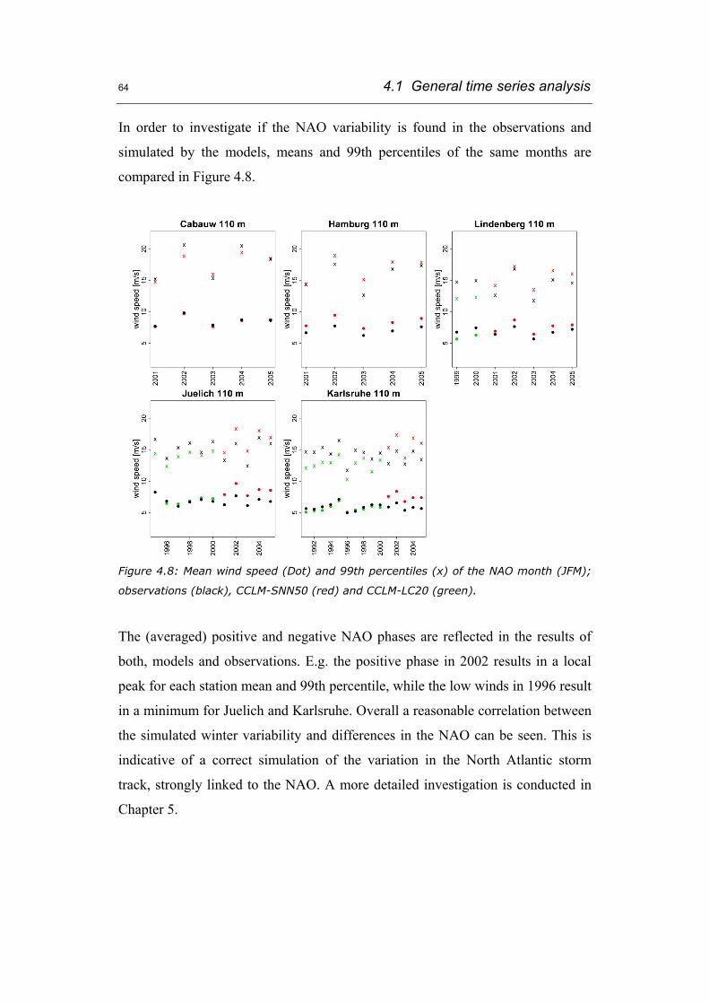
4.1 General time series analysis.................................................................50

4.1.1 Methods ......................................................................................50

4.1.2 Results and Discussion ...............................................................52

4.1.2.1 Annual cycle ....................................................58

4.1.2.2 Diurnal Cycle...................................................60

4.1.2.3 Interannual variability......................................62

4.2 Storm detection ....................................................................................65

4.2.1 Methods ......................................................................................65

4.2.2 Results.........................................................................................66

4.3 Summary and conclusions ...................................................................74

5 Trend analysis of simulated wind fields ...................................................77

5.1 Methods ...............................................................................................79

5.2 Results for Europe 1961 - 2000 ...........................................................80

5.3 Summary and conclusions ...................................................................86

6 Summary and outlook................................................................................89

List of Abbreviations ...........................................................................................93

List of Figures.......................................................................................................95

List of Tables ........................................................................................................99

References...........................................................................................................101

Appendix.............................................................................................................113

Acknowledgements ............................................................................................113

1 Introduction

1.1 Motivation and background

It has become common practise to use regional climate models (RCMs) to

simulate regional wind conditions when no measurements are available.

Furthermore, RCMs are used in order to predict possible changes and effects on

the regional wind climate and as such contribute to community understanding of

the impacts of climate change. Hindcast simulations - presenting the climate of

the past - are investigated for the existence of trends in the mean or extreme wind

climate. These Hindcasts are simulations with regional climate models driven by

global reanalysis products. They downscale the climate forcing to serve as input

for further geo scientific applications and impact studies for instance for storm

surge models or in ecological studies (Weisse et al. 2009).

The wind energy sector is becoming increasingly dependent on detailed

knowledge about the wind climate for the operation, design, sales and marketing

of wind turbines. Mesoscale simulations are increasingly been used for resource

assessment and considered to provide reasonable understanding of regional wind

conditions (e.g. Frank and Landberg 1997; Benoit et al. 2004).

Due to the limited number of reliable observations the verification of simulated

wind fields is a difficult task. So far the model skill regarding the reasonable

simulation of boundary layer wind fields is primarily investigated by means of

marine wind fields and/or near-surface observations. Smooth water surfaces

2 1.1 Motivation and background

provide a relatively good condition for the comparison with model grid boxes.

The verification of simulated wind fields over land, the main scope of this study,

bears a larger challenge. Previous comparisons are mainly based on near surface

measurements from meteorological stations, which are subjected to

homogenisation algorithms to derive local wind climate estimate.

The homogenisation of near surface observations is a very complex process. One

should always consider the station location and surrounding environment. The

influence of the nearest surrounding on wind speed measurements is demonstrated

for the station Helgoland in Chapter 1.2.

The extrapolation of modeled wind speeds from the lowest model level to 10 m

height as typical height of near surface measurements is also fraught with issues.

This study proposes a new approach to solving this problem. This approach

reduces the disturbances due to the surface in the observations by using data from

higher measurement sources (towers). Simply put, such data are less affected by

surface roughness and obstacles and are more representative of a larger area. In

addition, no extrapolation of modeled wind data is required. The occurrence of the

extrapolation error is avoided by comparing measurements with simulated values,

which were either interpolated between two model level heights or which were

extracted directly at the given model level heights.

Data sets from tall measurement towers are rare and therefore of significant

scientific value. Towers of this height are often privately owned and operated by

wind companies. For this study a data base of five anemometer towers could be

established. Together they offer insight into regional conditions for different

terrain complexity. This database, the towers and their geographical context and

mesoscale models used in this thesis are discussed in Chapter 2.

In Chapter 3 two fundamentally different modeling approaches to downscale

mean wind, wind speed distribution and wind direction distribution profiles are

1.2 Quality of near surface measurements 3

compared. COSMO-CLM is a regional climate model using a dynamical

downscaling technique while the Wind Energy Simulation Toolkit (WEST) uses a

statistical-dynamical downscaling approach. The more computationally efficient

model, WEST, allows a detailed investigation of the influence of boundary

conditions like the roughness field and the forcing data. Furthermore, WEST’s

computational efficiency allows the modeler to increase the spatial resolution of

the modeling domain in this study up to 1 km. On the other hand WEST is not

able to simulate time series. Therefore, only time series from two COSMO-CLM

simulations are used to determine the temporal simulation skill in Chapter 4.

Wind speed variations as well as extreme values are analyzed.

After evaluating the performance of COSMO-CLM on temporal scales, a trend

analysis is conducted in Chapter 5. Trends of annual mean wind speed and 99th

percentiles are compared for two RCM simulations and their forcing reanalyses.

The scope is to see, if both reanalyses show similar trend patterns of the mean and

extreme wind speed and to what extent these patterns are reproduced in the

RCMs. A piecewise trend analysis for wind speed over Europe over the period

1961 - 2000 is conducted, considering possible changes in the wind climate

related to atmospheric large scale conditions.

1.2 Quality of near surface measurements

Near surface wind measurements are a common source of information for studies

in the wind energy sector and also in ecological, actuarial and meterological

related studies. Despite known problems with the homogeneity and the

representativity of measured wind data series (Wieringa 1996; WMO 2008), wind

measurements from near surface weather stations are used in several studies (for

example for wind farm sitings based on wind atlases (Troen and Petersen 1989) or

for verifications of simulated marine wind fields). The main focus of this chapter

is to background on the impact of the land surface on observed wind speed data.

4 1.2 Quality of near surface measurements

For this purpose, information about the former and present status of a number of

stations, shown in Figure 1.1, is used as an example and to highlight the influence

of sites location on its wind observations. Wind speed time series from five

stations are considered. These stations are part of the synoptic measuring net

(SYNOP) of the German Meteorological Service (DWD).

Figure 1.1: Positions of the chosen stations along the coasts of the German Bight.

Selection criteria for these sites are (a) similar temporal availability and (b) the

short distance to the North Sea coast and (c) close proximity to each other.

Accordingly, the stations should more or less exhibit the same regional wind

climate and similar relationships as to temporal variation can be expected for the

stations.

Meteorological data for forecast purposes are called SYNOP, as they are observed

synchronous. The data are observed hourly, resp. three- or six-hourly. The data of

wind speed are averages over ten minutes. A common observation period of 53

years (from 1953 to 2005) is covered with data for all five stations. The measuring

frequency of the SYNOP net changed from three-hourly to hourly records in 1978

(Behrendt et al. 2006). However, a continuous hourly sampling frequency since


1979 was only found for the stations Helgoland and Bremerhaven. The other

stations show gaps especially at night or at particular hours (e.g. at 7 and 8 pm).

Consistent hourly records started in Cuxhaven in 1987 and in Norderney and List

since 1989. Before the temporal adjustment the sampling frequency varied from 3

to 8 times a day, often only covering day time. The unit of the wind speed and the

accuracy changed from knots to m/s in October 1998 and to 0.1 m/s in April 2001

(Behrendt et al. 2006).

The yearly means and 99th percentiles of the wind speed of the five stations from

the SYNOP records show a low similarity (Figure 1.2 and Figure 1.3).

1960 1970 1980 1990 2000

4

5

6

7

8

9

Yea

rly m

eans

of w

ind

spee

d [m

/s]

Helgoland

List (Sylt)

Cuxhaven Norderney

Bremerhaven

Figure 1.2: Yearly means of wind speed measurements from five synoptic near coastal

stations: Helgoland (red), List (blue), Norderney (green), Cuxhaven (light blue),

Bremerhaven (purple). Shaded lines label years with known station relocations.


1960 1970 1980 1990 200010

12

14

16

18

20

99th

Per

cent

iles

of w

ind

spee

d [m

/s]

Helgoland

List (Sylt)

Cuxhaven Norderney

Bremerhaven

Figure 1.3: Yearly 99th percentiles of wind speed measurements from five synoptic

near coastal stations. Helgoland (red), List (blue), Norderney (green), Cuxhaven (light

blue), Bremerhaven (purple). Shaded lines label years with known station relocations.

Except of similar small scale variations between the time series of some stations

no common general large scale tendency can be identified, although the wind

conditions should be dominated by similar regional wind regimes and are

expected to reflect the same regional wind climate.

Comparisons with yearly means and 99th percentiles of the FF net, which is

homogeneous in sampling time and unit, show that changes in sampling frequency

and unit have a negligible effect and do not explain the large variations in the time

series.

The similar small scale behaviour between some stations at least indicates

consistent short term trends. E.g. at Helgoland and List a quite similar curve shape

can be observed in the yearly means neglecting the abrupt increase in 1990 in the

Helgoland data. This increase in wind speed is caused by a station relocation.


The station histories (Appendix A1) reveal that each of the stations was relocated

at least once during the considered time period. These relocations are not only

restricted to changes in location and therewith the environment. Changes of the

anemometer height, which varies between 10 and up to 28 m above ground level

(AGL) for the five stations, also play a decisive role.

The years with relocations or changes of the anemometer height are marked with

dashed lines in Figure 1.2 and Figure 1.3. Not surprisingly, they often result in

abrupt increases or decreases of the yearly mean and of the 99th percentiles. E.g.,

the abrupt decrease in the yearly means and in the yearly 99th percentiles of

Norderney from 1981 to 1982 occurs directly after a station relocation including a

change in the measuring height from 21 to 12 m AGL in September 1981.

At the station Helgoland an increase of 1.25 m/s is seen in the means of the

10 years before and after the year with the relocation (1989), even though the

measuring height changed from 15 to 10 m above ground level and from 19 to

15 m above mean sea level.

To illustrate the strong influence of the environment on wind measurements and

therewith the possible magnitude of the effect of a station relocation on the

measurements, a detailed investigation for the station Helgoland is conducted.

Helgoland consists of the “Unterland”, the flat area around the port, the

“Oberland”, elevated with a mean height of 50 m, and the Dune. Figure 1.4 shows

a map of Helgoland and the last three positions of the wind measurement station

at the southern port, the airport on the dune and the mole.


Figure 1.4: Position of the wind masts on the island of Helgoland since 19641

From February 1964 to November 1989 the wind speed was recorded from a

tower in the South of the port close to the meteorological station building in a

distance of approx. 375 m to the edge of the “Oberland” (Schmidt et al. 1993). In

the opposite direction the building of the station influenced the data until this

tower was damaged in November 1989. Therefore, data from the tower close to

the airport, on the dune, have been used as substitute for almost one month.

Afterwards, data from the tower at the end of the southern mole are used. The

distance of this new position to the edge of the “Oberland” is now larger than

1 km. The measurements are obviously much less disturbed than the

measurements located in the port, where the “Oberland”, the observatory and the

other buildings and facilities strongly influenced the observations. This resulted in

reduced wind speeds indicated by the lower yearly means and the lower 99th

percentiles before 1989, even though the height of the anemometer was 5 m

higher above ground level at the Tonnenhof station. Thus, higher wind speeds

would be expected for the first period. Especially the north westerly winds must

have been strongly disturbed by the shape of the “Oberland”. The measurements

from the dune, usually taken for quality controls of the main measurements (port

1 Map based on: www.openstreetmap.org, License: Creative Commons Attribution-Share Alike 2.0 Openstreetmap


and mole), are affected by a higher roughness because of the drag of the airport

facilities and the surface of the island. Assuming instrumental effects are

negligibly small, the differences between the wind records at the positions can be

attributed to the different environments.

The influences of the station relocations show the high sensitivity of the wind

measurements to changes in the environment. By using near surface wind

measurements as representatives for wind fields for any purpose, a valuation of

the homogeneity of these data should be conducted, as Wieringa has already noted

in his golden rule “never to use wind data from unspecific locations” (Wieringa

1996). Requesting the station’s metadata from the provider of the data is

compulsory. The occurrence of differences between measuring nets must be

considered. The metadata give a first impression of the homogeneity of the time

series. In cases of relocations these changes should be reported and can be found

in the station history. However, slowly developing changes in the environments

like vegetation growth or building of facilities close to the wind measurement

stations are usually not reported and hard to detect in most cases. Therefore, more

detailed information about the environment of former and present locations is

necessary. Approaches to achieve homogenization of wind data by means of such

information about station environment and more precisely the roughness length

and fetch (e.g. Wieringa 1976; Wieringa 1996; van der Meulen 2000) can help to

increase the reliability of the measurements. Such homogenization approaches

were applied for the stations Helgoland (Niemeier and Schlünzen 1993) and

Norderney (Schmidt and Pätsch 1992). The application of such is unavoidable

before using near surface wind measurements. Homogenization processes may

become quite complex and require detailed information about the anemometer

locations and meteorological expertise.

The existence of errors in wind statistics due to the inhomogeneity of the input

data can not be ruled out. They are indeed most likely.


Comparisons with yearly means and 99th percentiles from four other near coastal

stations show that this is not a single and a “worst” case scenario. All stations

were affected by at least one station relocation during a period of 44 years. In

most of the cases these station relocations led to a detectable sudden increase or

decrease in the yearly means and yearly 99th percentiles.

There are reasonable alternatives to the direct use of measured wind data. One is

the use of wind proxies derived from pressure measurements, which are not

sensitive to influences of the environment (e.g. Schmidt and von Storch 1993).

Another possibility is the use of data from tall measurement towers. These

measurements are not affected by station relocations and they are much more

homogenous also due to the strongly decreased influence of the environment.

2 Data sets

2.1 Tower measurements

Analysis of measurements from synoptic stations (with measuring heights around

10 m) show that they are often not representative over large areas and for

comparisons with simulated winds in grid boxes of low spatial resolution without

homogenization (Chapter 1.2; Wieringa 1976; Wieringa 1983). To reduce the

influence of the disturbances due to the environment, measurements from five tall

meteorological towers are used in this study. The data sets were provided by

different research institutions.

A brief description of the towers and their surroundings is given in Table 2.1. The

environments of these towers and therefore the simulated areas vary in complexity

of terrain structure and land use. Cabauw is located in a homogenous flat area and

Lindenberg is surrounded by agricultural fields and small forests. The Hamburg

tower is located in an industrial area of the city. Cabauw, Lindenberg and

Hamburg have comparably simple conditions for the simulation of mean wind

fields. In contrast, the conditions at the sites Juelich and Karlsruhe are quite

different as both towers are located in forests. Juelich in a broad leaf forest and the

site Karlsruhe features predominately coniferous species and a more complex

terrain structure. At both of these sites land use parameterisation and orography

play an important role on the simulations.

12 2.1 Tower measurements

Table 2.1: Description Tower Measurements

Station ASL: Owner: Environment Starting time

Hamburg 0.3 m University of Hamburg Land cover: Suburban, flat

industrial area; rather

homogeneous orography

01.2001

(UltraSonic)

Cabauw -0.3 m Koninklijk Nederlands

Meteorologisch

Instituut (KNMI)

Grasslands, agricultural and small

villages;

open and flat terrain

05.2000

Lindenberg 73 m Richard-Aßmann-

Observatory, German

Meteorological Service

Mixed land cover: arable fields and

small forests

06.1998

Juelich 91 m Research Center

Juelich

Located in a small clearing in a

broad leaf forest, surrounded by

research Center facilities

01.1995

Karlsruhe 110 m Research Center

Karlsruhe

Needle-leaf forest, surrounded by

research Center facilities

Located in the Upper Rhine valley

01.1974

For a better illustration the towers are separated into two groups according to the

complexity of terrain and land use:

• Northern stations:

Flat/homogenous terrain: Cabauw and Lindenberg and urban: Hamburg

• Southern stations:

Complex terrain/forests: Juelich and Karlsruhe

Outliers are removed from the observations and data adjusted to remove the

influence of the tower ensuring error as small as possible. Either the tower has

more than one measuring arm or the data are removed in cases in which the wind

comes from the mast direction.

To reduce the influence of the immediate surroundings the main focus of this

analysis is on results at and above 50 m heights.

2.2 Model data 13

Table 2.1 shows that data from all towers are available for the period 2001 - 2005.

No major gaps are found for this period. Therefore, representative measurements

over the period (2001 - 2005) can be ensured for the chosen stations and heights.

This period serves as reference period for the verification of mean wind statistics

and the sensitivity analysis presented in Chapter 3. Due to a deviating simulation

period of one of the RCM simulations, covering 1991 - 2000, also a second period

is chosen for the time series analysis in Chapter 4. The second period differs for

the towers depending on the availability of the measuring data after 1991 and

before 2001 (Table 2.1). E.g. for Karlsruhe, the whole 10 years are covered, while

the data from Cabauw are starting in May 2000. Furthermore, some longer gaps

are found in this period.

2.2 Model data

2.2.1 Reanalysis data

Reanalysis data are a combination of different kinds of observations e.g. data from

weather stations, buoys, radiosondes and satellite images assimilated into modern

prediction models. The assimilation scheme provides for a uniform spatial and

temporal coverage and a gridded dataset. Because reanalysis data are based on

observations they are subject to changes in time and space and should not be seen

as absolute reliable representatives of the true climate (Kistler et al. 2001;

Reichler and Kim 2008).

NCEP/NCAR Reanalysis 1 (NCEP)

The 10 m wind speed derived from wind components in zonal and meridional

direction of the NCEP/NCAR Reanalysis 1 is used for the trend detection

analysis. The data are provided by NOAA/OAR/ESRL PSD, Boulder, Colorado,

USA2. Starting 1948 it contains 6 hourly model output. The 10 m wind speed

2 http://www.esrl.noaa.gov/psd

14 2.2 Model data

components are available on a global T62 Gaussian (~1.875°) grid. A detailed

description of the NCEP/NCAR Reanalysis 1 is given in Kalnay et al. (1996).

ERA40 Reanalysis (ERA)

In addition ERA40-Reanalysis data are investigated within the trend detection

process. 10 m wind components of the reanalysis data of the European Centre for

Medium-range Weather Forecasts (ECMWF) are available on a 1.125° grid for

the period 1958 - 2002 with an output interval of 6 h. A detailed description can

be found in Uppala et al. (2005).

Japanese 25-year Reanalysis (JRA)

The JRA reanalysis was conducted by the Japan Meteorological Agency (JMA) in

collaboration with the Central Research Institute of Electric Power Industry

(CRIEPI). The data set has a spatial resolution of ~120 km (T106 grid) covering

the period 1979 up to the present (Onogi et al. 2007). Data over the period 2001 -

2005 are used for the sensitivity analysis in Chapter 3.

2.2.2 Regional Climate Model data

SN-REMO

In this study data of a simulation with the hydrostatic regional climate model

REMO (REgional MOdel, Jacob and Podzun 1997) by Feser et al. (2001) is used

for the trend detection. REMO is based on the Europa-Modell (EM) from the

German Weather Service. 10 m wind speeds are taken from a Hindcast

simulation, covering the period 1948 - 2006. The simulation was done on a

rotated grid that covers Europe with a spatial resolution of 0.5° x 0.5° and 20

vertical levels.

For this Hindcast simulation REMO 5.0 was forced by the NCEP/NCAR-

Reanalysis 1 and NCEP/NCAR-Reanalysis 2 after 03/1997 at the lateral

boundaries and within the domain by a spectral nudging approach influencing the

2.2 Model data 15

wind components of the upper layers (von Storch et al. 2000). The spectral

nudging approach includes an assimilation of large scales from the reanalysis,

spectrally composed, to the wind components of REMO (Feser and von Storch

2005). Therefore it forces the RCM closer to the large scale behaviour of the

reanalysis. The nudging starts at the top of the model and the coefficient decreases

with height to 850 hPa. This gives the RCM more freedom for lower heights,

where regional features have higher influence and an added value due to the

higher resolution of the RCM is expected.

COSMO-CLM

The regional climate model COSMO-CLM (Böhm et al. 2006) is the climate

version developed from the non-hydrostatic Local Model (COSMO) of the

German Weather Service (DWD) by the CLM community3. Details about the

physical parameterizations, dynamics and numerics of the model can be found in

Doms et al. (2005), Doms and Schättler (2002) and Schulz (2009). Within this

study three different simulations are used:

CCLM-SNN50

For this study data of version 3.21 from a simulation by the GKSS Research

Center Geesthacht is taken for the verification of simulated mean wind statistics

and the sensitivity analysis in Chapter 3 as well as for the verification of time

series in Chapter 4. The simulation area covers Europe and uses a rotated grid

with a spatial resolution of 0.44° x 0.44° (~50 km), 32 vertical levels, and an

output interval of 3 hours, covering 2001 - 2005. The simulation is spectrally

nudged with the NCEP/NCAR-reanalysis 1.

CCLM-SNE50

For the trend analysis 10 m wind speed from a simulation of Version 3 (2.4.6)

from the ENSEMBLES project is used (Hewitt and Griggs 2004). This simulation

3 www.clm-community.eu

16 2.2 Model data

has the identical spatial resolution of 0.44° x 0.44° (~50 km) and 32 vertical

levels, but it has the higher output interval of 1 h. The simulation is spectrally

nudged by ERA 40.

CCLM-LC20

Within the LandCare 2020 project (Köstner et al. 2009) a simulation of COSMO-

CLM 2.4.11 with a spatial grid resolution of 0.165° x 0.165° (~ 20 km) was

conducted, forced at the boundaries by NCEP/NCAR Reanalysis 1 but not

spectrally nudged. It has 32 vertical levels and an output interval of 3 hours over

the period 1991 - 2000. This simulation is used for the time series analysis in

Chapter 4.

Wind Energy Simulation Toolkit (WEST)

The Wind Energy Simulation Toolkit uses a statistical-dynamical downscaling

approach described in Frey-Buness et al. (1995) and Mengelkamp (1999). A

classification of geostrophic wind data from a forcing data set is conducted. Mean

geostrophic wind and temperature profiles for each class are used as initial

conditions at the center of the chosen domain (Yu et al. 2006). A mesoscale model

simulation with the Canadian Mesoscale Compressible Community Model MC2

(Tanguay et al. 1990 and Thomas et al. 1998) is conducted for each class. The

results are weighted by the frequency of the occurrence of the class in the forcing

period. A statistical module calculates mean fields which can be seen as

representatives for the mean wind fields over the whole forcing period (Pinard et

al. 2005). The low computational effort allows a flexible application of the model

and a detailed investigation of the influences of the general settings. In the default

version the model is driven by the NCEP/NCAR-reanalysis (Kalnay et al. 1996).

3 Verification of simulated wind statistics

The wind power industry has grown steadily during the recent years and

constantly requires more reliable and detailed information on the wind climate on

local and regional scales. As modeling improves it increasingly becomes the

chosen alternative to near surface observations (e.g. Larsén et al. 2008). In this

chapter it is investigated, if limited area models are able to reliably simulate

boundary layer wind statistics over different land cover and terrain structures. In

contrary to common approaches, i.e. using surface observations, measurements

from tall towers are used.

The influence of the grid resolution, of the roughness lengths, and of the synoptic

climatological forcing is investigated. Simulated wind statistics from two models

with different downscaling procedures are compared. The differences in terrain

height and land cover structure between the sites allow a closer analysis of the

influence of the model grid environment. The simulations chosen for this

investigation are CCLM-SNN50 (dynamical downscaling) and the Canadian

Wind Energy Toolkit WEST (statistical-dynamical downscaling). State of the art

wind mapping systems as WEST are a common tool for the prediction of the wind

energy potential due to their less expensive application. They are often used for

the design of wind resource maps. A Canadian Wind Atlas with a resolution of

5 km was generated with WEST and its validation shows reasonable results for

different regions of Canada (Benoit and Yu 2003). A similar approach, based on

18 3 Verification of simulated wind statistics

the mesoscale model KAMM, was used for modeling the climate of Ireland

(Frank and Landberg 1997).

Wind atlases for Denmark, Ireland, Portugal were generated by means of a

combination of KAMM and the wind atlas analysis and application program

WAsP (Frank et al. 2001).

One major issue in the use of mesoscale models for the wind field simulation is

the selection of an adequate grid resolution. It is assumed that with higher

resolutions smaller scales can be reproduced. Thus, an added value for increasing

grid resolution is expected. This is most important over more complex areas.

The statistical-dynamical downscaling approach is more computationally efficient

than the dynamical downscaling approach. Therefore, WEST enables an

investigation of an added value for increased grid resolution. Furthermore, the

influence of the synoptic forcing and the land use on wind statistics (in particular

mean wind profiles, wind speed distributions and wind direction distributions) is

investigated.

WEST model simulations for Western Europe with typical mesoscale resolutions

of 50, 20 and 10 km are conducted and are compared to the observational data and

calculated mean fields of CCLM-SNN50 (~50 km resolution) for 50 and 100 m

AGL. To consider the complex terrain and land structures of the southern stations,

also high resolution (1km) WEST simulations are generated. Two reanalysis data

sets (NCEP/NCAR Reanalysis (NCEP) (Kalnay et al. 1996) and the Japanese 25-

year Reanalysis Project JRA-25 (JRA) (Onigi et al. 2007) are used as forcing data

for WEST. Distortions due to differences of Canadian and European land use

definitions are investigated by means of the USGS land use data, the CCLM-

SNN50 roughness field and the European land use database CORINE.

3.1 Methods 19

3.1 Methods

Wind statistics for the period 2001-2005 are calculated for all towers using the

output time interval from the CCLM-SNN50 model (three hours). The CCLM-

SNN50 output represents instantaneous wind speeds averaged over the model

time step of four minutes. Comparisons between mean wind fields from three-

hourly values (averaged over five, ten or twenty minutes) and from values with

the original measuring frequency, every five or ten minutes, reveal that adjusting

the time step has such a small effect on the mean wind fields of the observations

that deviations to the time steps of the WEST simulations can be neglected (not

shown).

The measured wind statistics for the period 2001 - 2005 are assumed to be

representatives for the true mean condition of the wind fields in the lowest 100

meter of the boundary layer. Simulated wind statistics over the same time period

are taken from the output of the CCLM-SNN50 simulation and from WEST. A

bilinear interpolation of the four tower surrounding grid points is used. For

Cabauw only the three surrounding land boxes of the CCLM-SNN50 data are

considered and an Inverse Distance Weighting is applied.

Mean wind speeds at 50 and 100 m height and their standard deviations are used

for the analysis. In addition, wind speed frequency distributions at both heights

are investigated after calculating the probability density functions (PDF).

According to WEST the wind speed is therefore classified into 27 wind speed

classes, each of them in the range of 1 m/s except of the first two and the last

class. The first class represents the calm situations between 0 and 0.2 m/s, the

second class the low wind speeds between 0.2 and 1 m/s. Wind speeds higher than

25 m/s are assigned to the last class (CHC 2006). The deviations between

measured and simulated wind speed distributions are expressed by statistical skill

scores as indicators for their similarity. A modification of the Perkins Score

(Perkins et al. 2007), which is also known as histogram intersection index HI, is

calculated for all simulations.

20 3.1 Methods

It is defined as

=

−=n

isimuobs hhHI

1

),min(1 (3.1)

with n equals the number of bins and hobs and hsimu as observed and simulated

smoothed frequencies of the bins of the PDFs. The HI score subtracts the overlap

of the simulated and observed PDF from One, so that the HI score equals zero for

a perfect simulation of the observed PDF. This score is biased to the median wind

speed classes. This means, it is more focused on deviations in the more frequent

median wind speeds. In addition, another, unbiased skill score is calculated, which

is more sensitive to deviations in the less frequent wind speed classes. The Chi2

score

( )

=

−=

n

i obs

obssimu

h

hh

1

22χ (3.2)

(with the same notation) weights the squared difference of two bins by the

frequency of the bin in the observations. It is also equal to zero for a perfect

simulated PDF.

The observations are partly logarithmically interpolated to the model level heights

of 50 and 100 m. The limited validity of the logarithmic wind speed law to near-

neutral cases is therefore ignored in agreement with WEST.

According to WEST the mean wind direction distributions are obtained by

classifying the wind directions into twelve sectors each representing an angle of

30° (CHC 2006).

3.2 Results and Discussion 21

3.2 Results and Discussion

3.2.1 Comparison CCLM-SNN50 and WEST

Initially, the general performance of both models is tested by choosing the

standard parameterization and default initial conditions of WEST and a spatial

resolution of 50 km.

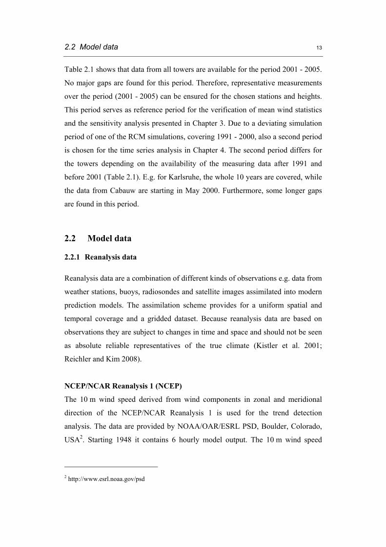
Northern stations:

The low resolution simulations (~50 km) of CCLM-SNN50 and WEST generate a

reasonable simulation of the mean wind profile for Cabauw (with

deviations < 0.4 m/s), but show a systematic overestimation of the mean wind

profile in Hamburg (> 0.5 m/s). For Lindenberg a good simulation can be reached

with CCLM-SNN50 instead of the large overestimation (of more than 0.8 m/s)

simulated by WEST (Figure 3.1). The WEST simulation shows, in contrary to

CCLM-SNN50, an overestimated variability, indicated by higher standard

deviations.

For the three northern stations the HI score of the CCLM-SNN50 simulation is

below 0.1 (Figure 3.2 a), describing an overlapping area between measured and

simulated PDF of more than 90 %. The best simulation is obtained for Cabauw

with an overlap of 93.3 and 96.8 %. The size of the overlap for the WEST

simulation ranges between 84.9 and 90 % for these stations (Table 3.1). The Chi2

score is close to Zero (< 0.041) for the CCLM-SNN50 simulation for the northern

stations and comparatively higher (between 0.047 and 0.359) for the WEST

simulation, indicating a worse simulation of the less frequent wind speed classes

by WEST (Figure 3.2 b).

22 3.2 Results and Discussion

50 mW

ind

spee

d [m

/s]

US

GS

CO

R.

CC

LM z

0

JRA

US

GS

CO

R.

CC

LM z

0

JRA

US

GS

CO

R.

CC

LM z

0

JRA

US

GS

CO

R.

CC

LM z

0

JRA

US

GS

CO

R.

CC

LM z

0

JRA

0

1

2

3

4

5

6

7

8

9

10

11

12

13

Obs

.

CC

LM

Obs

.

CC

LM

Obs

.

CC

LM

Obs

.

CC

LM

Obs

.

CC

LM

WEST WEST WEST WEST WEST

Cabauw Hamburg Lindenberg Juelich Karlsruhe

Obs.CCLM-SNN50

WEST USGSWEST CORINE

WEST CCLM-z0WEST CCLM-z0 JRA

100 m

Win

d sp

eed

[m/s

]

US

GS

CO

R.

CC

LM z

0

JRA

US

GS

CO

R.

CC

LM z

0

JRA

US

GS

CO

R.

CC

LM z

0

JRA

US

GS

CO

R.

CC

LM z

0

JRA

US

GS

CO

R.

CC

LM z

0

JRA

Obs

.

CC

LM

Obs

.

CC

LM

Obs

.

CC

LM

Obs

.

CC

LM

Obs

.

CC

LM



0

1

2

3

4

5

6

7

8

9

10

11

12

13 Obs.CCLM-SNN50

WEST USGSWEST CORINE

WEST CCLM-z0WEST CCLM-z0 JRA

Figure 3.1: Observed and simulated mean wind speeds and their standard deviation

(2001 - 2005) a) at 50 m and b) at 100 m, simulated with a spatial grid resolution of

50 km. Per station from left to right: CCLM-SNN50, WEST simulations: with USGS land

use, with CORINE land use, with the CCLM roughness field and forced by NCEP and

with the CCLM roughness field and forced by JRA.

a)

b)


Figure 3.2: a) HI Scores and b) ChiP

2P Scores for the simulated PDFs with a spatial grid

resolution of 50 km. Per station from left to right: CCLM-SNN50 (CCLM), WEST

simulations: with USGS land use, with CORINE land use, with the CCLM roughness

field and forced by NCEP and with the CCLM roughness field and forced by JRA at 50 m

(Point) and at 100 m (x).

HI S

core

00.

10.

20.

3

CC

LM

CC

LM

CC

LM

CC

LM

CC

LMUS

GS

CO

R.

CC

LM z

0

JRA

US

GS

CO

R.

CC

LM z

0

JRA

US

GS

CO

R.

CC

LM z

0

JRA

US

GS

CO

R.

CC

LM z

0

JRA

US

GS

CO

R.

CC

LM z

0

JRA

US

GS

CO

R.

CC

LM z

0

JRA

US

GS


50m100m


CH

I^2

Sco

re

00.

51

CC

LM

CC

LM

CC

LM

CC

LM

CC

LMUS

GS

CO

R.

CC

LM z

0

JRA

US

GS

CO

R.

CC

LM z

0

JRA

US

GS

CO

R.

CC

LM z

0

JRA

US

GS

CO

R.

CC

LM z

0

JRA

US

GS

CO

R.

CC

LM z

0

JRA

US

GS

CO

R.

CC

LM z

0

JRA

US

GS


50m100m


a)

b)

Tab

le 3

.1:

Siz

e of

the

ove

rlap

of

obse

rved

and s

imula

ted w

ind s

pee

d P

DFs

in p

erce

nt.

Cab

auw

H

ambu

rg

Lind

enbe

rg

Juel

ich

Kar

lsru

he

50m

10

0m

50m

10

0m

50m

10

0m

50m

10

0m

50m

10

0m

CC

LM-S

NN

50

50

93

.3

96.8

93

.4

90.3

92

.8

93.9

82

.6

84.5

75

.3

82.6

WES

T

50

USG

S 90

.0

88.6

89

.5

87.9

88

.1

84.9

75

.0

81.3

80

.4

85.9

C

OR

INE

88.7

87

.8

94.9

90

.3

93.1

92

.7

80.7

84

.7

85.3

90

.2

C

OSM

O-C

LM z

0 89

.2

88.8

92

.9

89.5

93

.0

92.6

78

.6

83.8

80

.4

85.7

C

OSM

O-C

LM z

0 JR

A

88.1

87

.5

95.9

90

.2

89.8

90

.5

81.7

85

.4

79.8

84

.2

20

USG

S 89

.8

89.2

90

.2

88.4

86

.6

84.6

77

.2

80.8

74

.8

78.3

C

OR

INE

89.7

90

.3

93.4

88

.7

91.7

89

.7

84.1

85

.0

80.9

84

.9

10

USG

S 89

.8

90.7

84

.9

88.3

84

.2

82.4

82

.7

82.8

74

.3

77.4

C

OR

INE

88.7

92

.3

94.7

91

.4

92.7

91

.1

85.5

82

.1

80.6

84

.7

1 C

OR

INE

90.8

91

.1

93.3

91

.5

92.1

92

.1

93.2

93

.0

92.1

94

.9


Both models reasonably simulate the wind direction distribution for Cabauw and

Lindenberg with a slight underestimation of the frequency of easterly winds for

WEST. This effect is shown for Cabauw in Figure 3.3.

a) Obs. 40 m b) CCLM 50 m c) WEST 50 m

Figure 3.3: a) Observed wind direction distribution in Cabauw (2001-2005). Simulated

wind direction distributions b) by CCLM-SNN50 and c) by WEST (50 km resolution).

The frequency of the main wind direction (W) in Hamburg is well simulated by

WEST but underestimated by CCLM-SNN50 and both models simulate more

south-westerly winds. A second peak in the wind direction distribution of

Hamburg, in south easterly winds, is simulated but underestimated (Figure 3.4).


Figure 3.4: a) Observed wind direction distribution in Hamburg (2001 - 2005).

Simulated wind direction distributions b) by CCLM-SNN50 and c) by WEST (50 km

resolution).

Southern stations:

Both models show a systematic overestimation of the mean wind speed for the

forest stations (> 1 m/s) with an extreme overestimation of more than 2 m/s for


Juelich at 50 m height by WEST (Figure 3.1). The lower variability of the wind

speed at Karlsruhe is seen but overestimated by both models. The overlapping

areas for the forest stations are comparatively small in a range of 75.3 - 84.5 % by

CCLM-SNN50 and 75 - 85.9 % by WEST (Figure 3.2 a and Table 3.1). Also the

Chi2 score for CCLM-SNN50 is larger (with values between 0.085 and 0.356) for

the forest stations in comparison to the results for the northern stations (Figure

3.2 b). With WEST the values for the Chi2 score are, in comparison to the

northern stations Hamburg and Lindenberg, not remarkably higher for the forest

station Karlsruhe with values of 0.108 and 0.322. At the other forest station,

Juelich, the Chi2 score reaches a size of 0.401 and 1.113.

The wind direction distribution of Karlsruhe is strongly influenced by the

orography. The wind is channelled due to the Upper Rhine valley with the main

directions between 195° and 225° and between 45° and 75° (Figure 3.5). The

complex orography is not resolved by the averaged fields in the models. CCLM-

SNN50 simulates the correct main wind direction of south westerly winds, but

with lower frequency, and underestimates the frequencies of east-north-easterly

winds. The frequency of all other wind directions is overestimated.


Figure 3.5: a) Observed wind direction distribution in Karlsruhe (2001 - 2005).

Simulated wind direction distributions b) by CCLM-SNN50 and c) by WEST (50 km

resolution).


The mean wind direction distribution of WEST shows more frequent westerly

winds and also an underestimation of the observed main wind directions (Figure

3.5).

Summary

Both models show a systematic overestimation of the mean wind speed for the

forest stations and for the urban station Hamburg. For the two other northern

stations over rather homogenous terrain CCLM-SNN50 reasonably simulates the

mean wind speed profiles, while WEST shows an overestimation at the station

Lindenberg. As detected for the simulation of the wind speed profile, the

deviations between observed and simulated PDF are mostly larger for the forest

stations.

The simulated profiles by WEST show a higher agreement with the observations

in three cases (at Karlsruhe at both heights and at Cabauw at 50 m). In the other

cases the simulated profile by CCLM-SNN50 is closer to the observations.

Comparing the performance for the simulation of the wind speed distributions by

both models shows smaller scores and therewith smaller deviations to the

observed PDFs with the CCLM-SNN50 simulation for four of the stations. Only

for the station Karlsruhe the simulated PDF by WEST is, as the wind speed

profile, closer to the observed PDF. The orography of both simulations is taken

from the GTOPO30 data set (USGS 2009). The CCLM-SNN50 roughness fields

show higher values for the grid boxes at Karlsruhe. Thus, differences are a result

of different model dynamics or downscaling methods.

Summarizing for all stations, the wind direction distributions for the northern

stations over comparably homogenous terrain can be reasonably simulated by

both models with an overestimation of southwesterly winds for one station. A

tendency towards an underestimation of the frequency of easterly winds is

generally found for both models, but is stronger in the WEST simulation. The


channelisation effect due to the Upper Rhine valley for the station Karlsruhe is,

however, not simulated by the models with the low spatial resolution.

3.2.2 Influence of the roughness field

The largest deviations between simulated and measured profiles for the stations

with more complex land cover possibly indicate an inadequate representation of

the roughness structures in the models (Note that in this study the terms roughness

and roughness length (z0) refer to the land use based roughness).

Within the preprocessing the model roughness lengths are generated by averaging

predefined roughness fields with different resolutions over the grid box areas. The

predefined fields are a result of land use definition routines. By means of satellite

images the land cover data are classified into land use classes. These land use

classes and the spatial resolutions of the map vary between different land use data

sets. In order to assimilate the land cover data to the model, the land use classes

are assigned to fixed land use classes of the respective model each with a specific

roughness length.

Beside the uncertainty of satellite measurements and deviations in the spatial

resolutions of different land cover data sets, major uncertainties occur within the

classification process. This includes the land use detection and classification

process, with uncertainties due to temporal variations or in the choice of training

data (Castilla and Hay 2007). But also the assignment to the model land use

classes is a critical point. Especially for the two latter points the consideration of

regional differences is important. Conceivably a European forest does not

necessarily match the definition of larger North American forests. Also roughness

lengths of similar vegetation forms can be regionally different.

In order to have identical roughness descriptions in both models, the roughness

fields are adjusted by interpolating the roughness lengths used by CCLM-SNN50


(based on ECOCLIMAP (Champeaux et al. 2005)) to the WEST 50 km grid. The

50 km simulation of WEST is repeated with the adjusted z0. To be able to

investigate the influence of the roughness fields also for higher resolutions, we

use the CORINE Land Cover 2000 (CORINE) (Bossard et al. 2000) data set with

a spatial resolution of 100 m instead of the original data USGS (with a spatial

resolution of 1 km) (Loveland et al. 2000). The CORINE data set consists of 44

different land use classes and covers Europe. These land use classes are assigned

to the 26 land use classes of WEST considering assignments from Silva et al.

(2007) and own considerations based on Stull (1988) and the specification of the

WEST land use classes (CHC 2006) and the tower environments. After this

classification, WEST simulations with a spatial resolution of 50, 20 and 10 km are

conducted with new roughness fields based on CORINE.

Since the wind direction simulation is mainly influenced by the orography no

effect of the replaced land use data set on the wind direction distributions is

found.

The development of the model roughness lengths of WEST with increasing spatial

resolution is shown in Figure 3.6. The roughness length based on USGS is smaller

than the one based on CORINE in all cases for all resolutions. The roughness

lengths from the interpolated CCLM-SNN50 roughness fields are mostly in

between. Only for Lindenberg the roughness length based on ECOCLIMAP is

slightly higher than the one based on CORINE.

The CORINE Land Cover data base should be advantageous to USGS due to a

higher spatial resolution and the European origin. This also holds for the CCLM-

SNN50 roughness field based on ECOCLIMAP. The effects of the differences on

the mean wind speed profile and on the wind speed distribution and the reliability

of the different roughness fields are evaluated in the following.


Figure 3.6: WEST roughness lengths in m based on CORINE (black) and USGS (grey)

for different resolutions. WEST roughness length based on the CCLM-SNN50 roughness

field ECOCLIMAP (X). Forest stations are marked with grey names.

Northern stations

Adjusting the roughness fields of WEST with the CCLM-SNN50 roughness field

lead to quite similar simulations of the mean wind profile by both models. This

results partly in a decrease in the simulation skill for Cabauw, with an

underestimation of the mean wind speed (Figure 3.1) and a decrease in the wind

speed PDF overlapping area at 50 m (Figure 3.2 a).

For Hamburg and Lindenberg the new roughness field reduces the mean wind

speed by up to 0.35 m/s and up to 0.9 m/s, respectively, and it increases the

overlap up to 3.9 and 7.7 % (Table 3.1). The overestimation of high wind speeds

can be reduced for all northern stations, as indicated by lower Chi2 scores (Figure

3.2 b). However, the overestimated wind speed variability of WEST is not

reduced.


Figure 3.7: a) HI Scores and b) ChiP

2P Scores for the simulated PDFs with increasing grid

resolution from 50 to 20 to 10 and to 1 km. Per station with CCLM-SNN50 (CCLM)

(black), WEST simulations: with USGS land use (red), with CORINE land use (blue), at

50 m (Point) and at 100 m (x).

CH

I^2

Sco

re

00.

51

1.5

2.5

CC

LM

CC

LM

CC

LM

CC

LM

CC

LM

50 20 10 1 50 20 10 1 50 20 10 1 50 20 10 1 50 20 10 150 20 10 1 50


CCLMWEST:USGSWEST:CORINE50m100m


HI S

core

00.

10.

20.

3

CC

LM

CC

LM

CC

LM

CC

LM

CC

LM

50 20 10 1 50 20 10 1 50 20 10 1 50 20 10 1 50 20 10 150 20 10 1 50


CCLMWEST:USGSWEST:CORINE50m100m


a)

b)


Replacing USGS by CORINE land use data leads to quite similar effects. Due to

higher values of the roughness lengths the effect is stronger for Cabauw and

Hamburg. This has again partly negative effects for Cabauw, especially at 50 m.

For Hamburg and Lindenberg it results in decreased scores in comparison to the

USGS land use for all resolutions. Increases in the overlapping PDF area up to 9.9

and 8.7 % respectively (Figure 3.7 a and Table 3.1) and lower Chi2 scores are

found for both stations (Figure 3.7 b). Opposite to the CCLM-SNN50 roughness

field, the simulation skill for the wind speed variability partly increases with

CORINE (Figure 3.8).

Southern stations

For Karlsruhe the effect of the CCLM-SNN50 roughness field is comparably

small due to the small difference in the roughness lengths (Figure 3.6): For Juelich

it helps to reduce the overestimation in the mean wind speeds up to 0.56 m/s and

increases the PDF overlap of 3.6 and 2.5 % (Table 3.1), respectively, and strongly

decreases the Chi2 scores (Figure 3.7).

With the 50 km resolution the higher roughness of CORINE results in a stronger

decrease of the overestimation of the mean wind speed for both stations and in

increases in the overlapping areas of the wind speed PDFs (up to 5.7 % (Juelich)

and 7.6 % (Karlsruhe), respectively (Table 3.1)). Also the effect on the

Chi2 scores is stronger as with the CCLM-SNN50 roughness lengths.

Similar effects can be observed for the higher resolutions (Figure 3.7 and Figure

3.8), where the higher roughness of CORINE reduces the wind speeds and

improves the simulations of the wind speed distributions. Only the 10 km

simulation constitutes an exception for the 100 m height at Juelich, where the

simulation with CORINE leads to higher wind speeds and therewith to a reduced

simulation skill.


50 mW

ind

spee

d [m

/s]

50 20 10 1 50 20 10 1 50 20 10 1 50 20 10 1 50 20 10 1

Obs

.

CC

LM

Obs

.

CC

LM

Obs

.

CC

LM

Obs

.

CC

LM

Obs

.

CC

LM



0

1

2

3

4

5

6

7

8

9

10

11

12

13 Obs. CCLM-SNN50 WEST USGS WEST CORINE

100 m

Win

d sp

eed

[m/s

]

50 20 10 1 50 20 10 1 50 20 10 1 50 20 10 1 50 20 10 1

Obs

.

CC

LM

Obs

.

CC

LM

Obs

.

CC

LM

Obs

.

CC

LM

Obs

.

CC

LM



0

1

2

3

4

5

6

7

8

9

10

11

12

13 Obs. CCLM-SNN50 WEST USGS WEST CORINE

Figure 3.8: Observed and simulated mean wind speeds and their standard deviation

(2001 - 2005) a) at 50 m and b) at 100 m with increasing grid resolution from 50 to

20 to 10 and to 1 km. Per station with CCLM-SNN50 (CCLM) (black), WEST

simulations: with USGS land use (red), with CORINE land use (blue).

a)

b)


Summary

Adjusting the WEST roughness length to the CCLM-SNN50 roughness field leads

to quite similar simulated profiles in both WEST and CCLM-SNN50. In addition,

it generally improves the simulation for all stations except for Cabauw, where the

USGS land use provides better results for the 50 m height and seems to be more

conform to the roughness of the environment. The differences between the

profiles with the old and the new roughness fields range from minimal 0.02 m/s

(at 50 m height in Karlsruhe) to maximal 0.9 m/s (at 50 m height in Lindenberg).

Analogous improvements can be detected for the wind speed distributions. Except

for Cabauw at 50 m, where the new roughness provides a larger HI score, and for

Karlsruhe, where the deviations between the two versions of the model roughness

fields are small, a better simulation can be reached with the new roughness field.

The differences in the HI Score range between 0.000 and 0.076, indicating

differences in the overlapping PDF areas from 0.0 to 7.7 %.

Comparing the results of the new WEST simulation with the results of CCLM-

SNN50 shows also a large similarity for the simulation of the wind speed

distributions. The sizes of the overlapping area are quite similar and not obviously

better for one model. The occurrence of less frequent high wind speeds is,

however, still better simulated by CCLM-SNN50 for four of the stations,

indicated by smaller values of the Chi2 score. Also the simulation skill regarding

the wind speed variability is higher for CCLM-SNN50.

With CORINE, the overestimation of the mean wind speed could be reduced in

most of the cases. In 25 of 30 cases (for all towers in both heights with all

resolutions) the new roughness fields provide a better approximation of the mean

wind profile. Four of the other five cases are found for Cabauw, as already seen

for the CCLM-SNN50 roughness field. The differences between old and new

profiles for the 50 km resolution have a range of 0.27 (Karlsruhe, 100 m) to

0.87 m/s (Lindenberg, 50 m). Additionally, the new land use data base provides a


better simulation of the wind speed distribution in the same 25 of 30 cases

(83.33 %) indicated by a decrease in both scores. The differences in the HI Score

range between 0.002 and 0.098, indicating differences in the overlapping PDF

areas from 0.2 to 9.8 %.

In comparison to the CCLM-SNN50 roughness field CORINE provides better

results for the simulation of the mean wind profile in 8 of 10 cases and of the

wind speed PDF in 7 of 10 cases for the 50 km resolution, especially for the

stations over more complex land structures.

In the case of the Cabauw tower, located over flat terrain, the default land use data

base USGS seems to be more representative for the low roughness of the

environment. In the other cases, the USGS data seem to underestimate the

roughness. This especially holds for the forest stations, located in densely

populated areas. Note, that the limited sample size only allows conclusions for

these five stations and should not be simply generalized. But the differences

obtained after replacing the land use data base show that not only the resolution of

the land use data set but also the suitability for the simulation area is a decisive

factor.

3.2.3 Influence of the spatial resolution

Because of the low computational effort, simulations of WEST with different

spatial resolutions can be conducted for both land use databases. An added value

due to higher spatial resolution and therefore a higher reproduction of complex

structures is expected. However, the differences between simulated wind profiles

obtained by the different resolutions 50, 20 and 10 km are relatively small and the

wind speed over more complex land structures is strongly overestimated even

with the 10 km resolution. To consider this complexity, high resolution

simulations of WEST with a resolution of 1 km based on CORINE are conducted

additionally. Each WEST simulation is driven by a climate table generated within


the classification process of the forcing data. It contains statistical information

about the geostrophic wind distribution over the forcing period (here: 2001 -

2005) at one grid point close to the grid center. While the simulations with 50, 20

and 10 km spatial resolution are conducted on one large grid for all towers, five

small grids are used for the simulations with 1 km resolution. Influences of

different climate tables for the five model regions of the 1 km simulation and

therefore a positive effect due to a higher representativity of the forcing data

tables on the smaller simulation areas cannot be clearly separated from the

improvements obtained by higher resolved model orography and land use. They

are, however, assumed to be comparatively small considering the small spatial

deviations of the geostrophic wind and regarding the results of Chapter 4.4.

Northern stations

Comparing the simulation skill for the northern stations no consistent

improvement can be detected for an increasing resolution. The only cases, in

which the deviation between simulated and observed mean wind speed decreases

continuously with increasing resolution from 50 to 20 and to 10 km can be

observed for the wind speed profile for Hamburg and for the median wind speed

classes of the wind speed PDF for Cabauw at 100 m, both with CORINE land use.

Additionally, the differences resulting from an increasing resolution are

comparatively small with a maximum difference of 0.39 m/s and 5.3 % for USGS

and 0.19 m/s and 2.7 % for CORINE, respectively (Figure 3.7 a, Figure 3.8 and

Table 3.1). The influence on the simulation of less frequent wind speed classes,

illustrated by means of the Chi2 score, is very small, with maximum effects of

0.114 for USGS and 0.024 for CORINE (Figure 3.7 b). Also the wind speed

variability changes only slightly (Figure 3.8).

Even a high spatial resolution of 1 km does not generally improve the simulation

skill. For Cabauw at 100 m and for Hamburg and Lindenberg at 50 m the high

resolution simulation shows larger deviations to the observed mean wind speed

(Figure 3.1) and wind speed distribution than the best of the low resolution


simulations (Figure 3.7 and Figure 3.8). This also holds for the wind speed

variability, which is partly too low.

The effect on the wind direction distributions is small for the low resolutions with

only slight deviations in particular sectors. The high resolution simulations result

in reduced westerly winds and an overestimation of south westerly winds for these

stations, as shown for Cabauw (Figure 3.9).

a) Obs. 40 m b) WEST 50 km c) WEST 20 km

d) WEST 10 km e) WEST 1 km

Figure 3.9: a) Observed and b) simulated WEST wind direction distributions at Cabauw

(2001 - 2005) with a spatial resolution of 50, c) of 20, d) of 10 and e) of 1 km. Land

use: CORINE, forcing: NCEP.

Southern stations

The simulations of the mean wind speed show continuous improvements for

Juelich at 50 m with increasing resolution for both land use data sets. At 100 m

the simulation skill partly decreases (Figure 3.1). This is also seen for Karlsruhe at

both heights. This is quite similar to the results for the wind speed PDF, where the

HI Score is consistently increasing for Karlsruhe and only partly decreasing for

Juelich (Figure 3.7 a). The variability increases remarkably from 50 to 20 km


(Figure 3.8). Also higher Chi2 scores are detected for both stations and heights for

the 20 km resolution. That means, a decrease in the simulation skill of less

frequent wind speed classes can be found for both stations. This is mostly

followed by a higher simulation skill due to an increased resolution of 10 km. The

Chi2 score is, however, only in one case smaller for the 10 km resolution than for

the 50 km resolution. In comparison to the effects on the northern stations, the

effect on the southern stations is much stronger with a maximum effect of 2.152

(USGS) and 0.311 (CORINE) (Figure 3.7 b).

In contrary, increasing the resolution to 1 km leads to highest simulation skills for

the mean wind speed and wind speed PDF for both stations: with a resisting

overestimation in Juelich of more than 0.5 m/s (Figure 3.1) and an overlapping

PDF area of 93 and 93.2 % (In comparison: 80.7 - 85.5 % for the low resolutions

with CORINE). In Karlsruhe a deviation of only 0.13 m/s and an overlapping area

of 92.1 and 94.9 % are found (In comparison: 80.6 - 90.2 % for the low

resolutions with CORINE) (Figure 3.7, Figure 3.8 and Table 3.1). Also the

overestimation in the wind speed variability is significantly reduced for both

stations.

Increasing the resolution has a positive effect on the mean wind direction

distribution at Karlsruhe (Figure 3.10). The channelisation of the wind due to the

Upper Rhine valley is much more distinctive for the higher resolutions. While the

20 km resolution already gives a good representation of the prevailing SWW and

SSW wind directions, the best approximation of the wind direction distribution is

obtained with a 1 km resolution.


a) Obs. 100 m b) WEST 50 km c) WEST 20 km

d) WEST 10 km e) WEST 1 km

Figure 3.10: a) Observed and b) simulated WEST wind direction distributions at

Karlsruhe (2001 - 2005) with a spatial resolution of 50, c) of 20, d) of 10 and e) of

1 km. Land use: CORINE, forcing: NCEP.

Summary

An increase of the resolution of WEST from 50 to 20 and 10 km does not

necessarily improve the simulation of the mean wind speed profile. It only

provides improvements in 10 of 20 cases for both roughness fields. Thus, a

general added value is not detected. After replacing the roughness fields, the

increasing spatial resolution improves the simulated wind profile in more cases

(12 of 20 (CORINE) vs. 8 of 20 (USGS)). The magnitude of the effects of

increasing the resolution from 50 to 20 to 10 km is, however, small. The

differences in the wind speed profiles obtained with the new land use data are

below 0.15 m/s for the increase to 20 km and below 0.26 m/s for the increase from

20 to 10 km. Comparing the differences between the 50 km and the 10 km

simulation, a maximal difference of 0.24 m/s can be detected. With the old land

use database the differences in the resulting wind profiles are comparably larger,

for Juelich almost reaching 1 m/s.


Increasing the spatial resolution to 1 km leads to a reasonable agreement between

modelled and measured wind profiles for four of the stations. The systematic

overestimation of the wind profile for Juelich could be reduced but still remains.

Although a higher roughness over the forests is used (Figure 3.6), it does not seem

strong enough for this station. One possible explanation for the overestimation is

that the trees act like a displaced surface. Establishing a displacement height (Stull

1988) would be a possible solution but is not realizable due to the low height of

the first model level.

Comparing these observations for the wind profiles to the results for the wind

speed distribution gives similar results. Increasing the resolution from 50 to 20

and from 20 to 10 km improves the wind speed distribution simulations in only 21

of 40 (52.5 %) cases for the Chi2 score and in 17 of 40 (42.5 %) cases for the HI

score. Split into an increasing resolution from 50 to 20 and an increasing from 20

to 10 km, it provides improvements in only 6 of 20 or 15 of 20 cases in the

Chi2 score and in 8 of 20 and in 9 of 20 cases in the HI score.

Increasing resolutions from 10 to 1 km produces clear and large improvements in

the wind speed distributions for the southern stations. This is additionally

indicated by improved wind speed variabilities for these stations. For the other

stations both skill scores are not consistently smaller for the 1 km resolution vs.

the best simulation of the low resolutions (50, 20 and 10 km). For these stations

no consistent positive effect can be related to increasing the resolution to 1 km

As seen for the mean wind profiles, good simulations of the wind speed

distributions for the northern stations can be reached with the low resolution

simulations. The increased resolution does not necessarily result in smaller scores

and therewith in more realistic simulations. Additionally, the deviations between

observed and simulated wind speed distributions for these stations are small

compared to the deviations for the forest stations especially with the low


resolutions. Only the very high resolution of 1 km can provide a reasonable

approximation of the wind speed distributions over complex land structures.

A similar effect can be detected for the simulation of wind direction distributions.

The low resolution simulations of WEST provide a reasonable simulation of the

wind direction distribution over even and flat areas by reflecting the main wind

directions and only slightly underestimating the frequency of easterly winds.

Increasing the resolution to 20 and 10 km has only a small effect on the wind

direction distributions. Effects of more complex structures (here shown for the

channelisation effect of the Upper Rhine valley on the measurement tower in

Karlsruhe) are not detected by the low resolution simulations of 50 km of WEST.

But an increase of the spatial resolution continuously improves the simulation of

this effect. So the high resolution simulation yields a reasonable performance of

the mean wind direction distribution for this station.

3.2.4 Influence of the external forcing

The model performance strongly depends on the reliability of the driving fields in

reproducing the true large scale conditions. This holds for both downscaling

approaches. Due to differences in their assimilation scheme and assimilated data,

regional differences between global reanalysis data sets occur (Reichler and Kim

2008).

The sensitivity of the Canadian model WEST to changes in forcing data is

investigated by replacing the classification of wind speed data from NCEP-NCAR

Reanalysis with a classification of the Japanese Reanalysis data set JRA (Japanese

25-year Reanalysis Project JRA-25, (Onogi et al. 2007)). Within the classification

a new climate table is generated. The climate table represents the geostrophic

wind speeds at one grid point close to the grid center. The 50 km simulation with

the CCLM-SNN50 roughness field is repeated with the new climate table based

on JRA.


Figure 3.11: Occurrence frequency of the surface geostrophic wind speed classes in

the climate tables of the forcing data sets NCEP/NCAR Reanalysis (left) and JRA

Reanalysis (right).

Differences in the climate table from both forcing data sets are small (Figure 3.11

and Figure 3.12). Apparently, the frequency of high wind speed classes is higher

in NCEP than in JRA at this grid point. The mean surface geostrophic wind speed

is larger for NCEP. The mean wind direction distributions of both climate tables

show prevailing winds from the south to west (180° - 270°) sectors. The

frequency of easterly winds is slightly higher in the JRA classification table than

in the NCEP classification table. This is also the case for the northerly winds. In

compensation, the frequency of southerly and south westerly winds is slightly

higher in the NCEP classification table.

NCEP JRA

Figure 3.12: Occurrence frequency of the surface geostrophic wind direction classes in

the climate tables of the forcing data sets NCEP/NCAR Reanalysis (left) and JRA

Reanalysis (right).


The smaller mean wind speed of the JRA climate table conforms to the behavior

of the simulated wind profiles (Figure 3.1). The model simulates a smaller wind

speed when forced by JRA than for the NCEP forcing.

Northern stations

The JRA forcing reduces the mean wind speeds in a range of 0.2 – 0.39 m/s for

the northern stations and therewith reduces the overestimation in Hamburg (at

both heights) and at Lindenberg (at 100 m). Existing underestimations of mean

winds speeds, as in Cabauw or Lindenberg at 50 m, are intensified (Figure 3.1).

Also the value of the Chi2 score increases for the latter cases (Figure 3.2 b). The

differences in the overlapping areas of the wind speed PDFs are in a range of -3.2

to +3 % with positive effects only for Hamburg (Figure 3.2 a and Table 3.1). The

general shape of the wind direction distributions remains unchanged. Only the

frequency of easterly winds is better represented by the JRA forcing.

a) Obs. 40 m b) WEST 50 m NCEP c) WEST 50 m JRA

Figure 3.13: a) Observed and b) simulated wind direction distribution at Cabauw

(2001 - 2005) by WEST with NCEP forcing and c) with JRA forcing. Both: CCLM-SNN50

roughness fields and 50 km resolution.

Southern stations

The effect on the mean wind speeds is comparatively smaller for the forest

stations with a reduction of the overestimation at Juelich of 0.2 m/s and 0.0 m/s

(100 m) and 0.07 m/s (50 m) for Karlsruhe (Figure 3.1). While the values of the

Chi2 score decrease for both, the values of the HI score increase for Karlsruhe

(Figure 3.2). The differences in the overlapping areas of the wind speed PDFs are

44 3.3 Conclusions

in a range of -1.5 to +3.1 % with positive effects only for Juelich (Table 3.1). The

effect on the wind direction distribution at Karlsruhe is, again, very small with a

small decrease in the frequency of westerly winds and a small increase in ESE

winds.

Summary

Summarizing the results for all stations, the JRA forcing improves the simulation

of the mean wind speed due to a reduction of the wind speed in six of ten cases.

For the wind speed distributions the new climatological forcing improved the

simulation, represented by a decrease in both scores, in only four of ten cases. The

effect on the wind direction distributions is mostly positive but small. The shapes

of the wind roses are similar. Only very small differences occur between the

frequencies, especially in the easterly winds. These are more frequent after the

replacement conforming to the direction distribution of the climate table.

In comparison to the effects of changing the roughness lengths (maximal

difference 0.9 m/s) the effect of the differences in the climate table on the mean

wind profile is small. The magnitude of the deviations between the simulated

profiles varies between a maximum difference of 0.39 m/s for the 100 m height in

Hamburg and no difference at 100 m height for Karlsruhe. The effects are more

distinctive for the northern stations over more homogeneous terrain. The effects

on the simulation of the wind speed distributions are in a range of 0.6 to maximal

3.2 % in the overlapping area of the PDFs.

3.3 Conclusions

A sensitivity analysis is conducted focusing on the influence of model roughness,

grid resolution, and forcing data on simulated wind statistics in the atmospheric

boundary layer. Two models with different downscaling procedures are compared

and the simulated wind statistics are verified by means of five year observation

data from five meteorological masts using the measured wind speed and wind

3.3 Conclusions 45

directions at 50 and 100 m height. One simulation is generated by the regional

climate model CCLM-SNN50 with a spatial resolution of ~50 km. The Wind

Energy Simulation Toolkit WEST is used for simulating mean wind fields over

the same period starting with the spatial resolution of the RCM and increasing the

resolution to 20, 10 and finally 1 km. To evaluate the influence of the model

roughness field, the roughness lengths of these WEST simulations are generated

by means of two different land use data sets (with different spatial resolution) and

the roughness field of the CCLM-SNN50 simulation additionally. Replacing the

forcing NCEP data by the Japanese Reanalysis JRA shows only small changes.

The low resolution simulations (~50 km) of both models show a similar behavior

after assimilating the CCLM-SNN50 roughness length to WEST. The mean

vertical wind speed profiles and the frequency of median wind speed classes in

the wind speed distributions differ only slightly. The stations in flat terrain and

relatively simple land cover are better simulated than the results for the stations

over more complex terrain, where the mean wind speeds are systematically

overestimated by both models. The frequency of less frequent wind speed classes

is better simulated by CCLM-SNN50 for four of the stations.

The most important findings of the sensitivity analysis are listed briefly below:

Land use:

The improvement in the wind speed simulation obtained due to the replacement of

the roughness lengths shows the strong influence of the roughness field on the

simulation of the mean wind speed profile and the wind speed distribution

independently from the resolution. Using the highly resolved (100 m) land use

database CORINE provides an improvement versus the land use database USGS

with a resolution of 1 km in 25 of 30 cases (for five towers, two heights and three

resolutions) for the mean wind profile and for the wind speed distribution. At one

station over homogeneous terrain the higher roughness based on CORINE partly

decreases the simulation skill. It is shown that a correct land cover data set is very

46 3.3 Conclusions

important for modeling of near surface wind fields. In this study not only the

higher resolution of the CORINE (Corine Land Cover 2000) database should

guarantee a higher accuracy than fields from the lower resolved data USGS. But

also the suitability for the simulation area is a decisive factor. Therefore, not only

the suitability of the land use data itself but also the assignment to the model land

use classes and their roughness definition should be verified. Due to differences

between international land cover definitions a correct assignment of land use

classes is necessary and a verification of the suitability of the roughness data is

strongly recommended.

Forcing data:

Restricted to this case and the grid point chosen in this study, the differences

between the two Reanalysis databases NCEP and JRA are small and have

therefore only small effects on the simulated wind statistics. The simulation skill

undoubtedly depends on the validity and representativity of the forcing data.

Small uncertainties in the climate table have a comparably low effect on the

simulated wind speeds and wind directions.

Resolution:

Wind fields over flat terrain and rather uniform land cover can reasonably be

simulated with a low resolution. The wind fields over complex terrain show

strong deviations for all “low”4 grid resolutions. In 50 % of all investigated cases,

increasing the resolution from 50 km to 20 km and 10 km does not lead to an

added value in the simulation of the mean wind speed profile.

Additionally, the increased resolution did not improve the simulation of the wind

speed distribution in 47.5 % or 57.5 % of the cases for the simulation of the wind

speed distribution, according to two skill scores. Furthermore, the changes are

4 50, 20 and 10 km

3.3 Conclusions 47

comparably small with a maximum of 0.26 m/s in the mean wind speeds with the

CORINE land use data base.

A simulation with a 1 km resolution provides large improvements for the mean

wind profiles especially over complex terrain. The high spatial resolution leads to

a reasonable agreement of modelled and measured wind profiles for four of the

stations. For one forest station the overestimation of the mean wind speeds can be

reduced with the high resolution but still remains. Similar arguments hold for the

wind speed PDF. A high resolution clearly improves the simulated wind speed

distribution over complex land cover and complex terrain structure. For the

stations over rather uniform terrain no added value for the simulation of the wind

speed PDF with the high resolution is detected.

Effects of complex orographic structures like the channelisation in the Upper

Rhine Valley are not detected in the 50 km simulation. The higher the resolution

the stronger the effect of the channelisation is reflected in the simulated wind

direction distribution. Over even and flat areas the low resolution simulations of

both models suffice for a reasonable simulation of the mean wind direction

distribution.

For very complex land cover structures like suburbs, forests or densely populated

areas or complex orographic structures an appropriate high resolution is

necessary. The resolution should be aligned to the complexity of the environment

otherwise an added value is not assured for additional computational effort.

4 Verification of simulated wind time series

The sensitivity analysis in Chapter 3 shows that an adequate representation of

surface terrain and land cover is crucial for a reasonable simulation of mean wind

statistics. In addition to reasonably simulated mean wind conditions a realistic

simulation of temporal wind variability is required e.g. for wind energy purposes.

Time series of wind speed are used in several areas: Not only in the wind energy

industry but also as input forcing for the simulation of other atmospheric or

ecologic processes (e.g. for storm surge models (e.g. Grossmann et al. 2007) or

for marine pollution models (e.g. Chrastansky et al. 2008)). Thus, a more detailed

investigation of the wind speed distribution and its mean temporal variation is

conducted and the skill of simulating extreme events is analyzed.

Because of its dynamic-statistical downscaling approach, WEST is not suitable

for the simulation of time series. Here, two COSMO-CLM simulations are

compared to the met mast´s wind measurements: the CCLM-SNN50 simulation

has a spatial resolution of 50 km, the CCLM-LC20 simulation of 20 km. Both

simulations use different nudging schemes and provide different simulation

periods (see Section 2.2.2).

50 4.1 General time series analysis

4.1 General time series analysis

4.1.1 Methods

The approach for comparing wind fields of both COSMO-CLM simulations with

met mast data is mostly similar to that described in Chapter 3.1. Again, wind

speed and wind direction time series are extracted from the tower data and from

the simulations using the output time step from both COSMO-CLM simulations

(3 h).

Two alterations to the former approach are made:

1. In order to eliminate uncertainties due to model interpolation routines, the data

are now taken directly at the model level heights at ca. 34 m, ca. 110 m and

ca. 203 m. The observational data are partly logarithmically interpolated

between the two neighbouring heights. The uncertainty induced by a simple

logarithmic interpolation is assumed very small because of the small vertical

distance between the measuring heights. In cases where the highest met masts

measurement is at 200 m, the wind speed is extrapolated to ca. 203 m using

measurements from the to highest observation levels.

2. Due to some large gaps in the observations before 2000 and due to different

starting times (Table 4.1), gaps in measurements and simulations were

adjusted. Hence, resulting wind statistics are not representative over the whole

reference period.

The wind fields of the COSMO-CLM simulations are to be considered as values

at a model grid box averaged over the model time step of a few minutes.

Observational data are twenty, ten or five minute averages at one specific point. In

order to investigate the influence of different averaging periods, observations at

Lindenberg with different averaging times (of ten minutes, of one hour, of three

hours) at the output time of the model (every three hours) are compared to the

simulated values of CCLM-SNN50. The difference between the three

4.1 General time series analysis 51

observational time series is much smaller than their deviation to the simulation.

This is supported by only small differences in the statistical scores between

observations and simulation: The correlation coefficient between observation and

simulation does not change for different averaging times. Differences of 0.01 m/s

are found between the Bias and RMSE of the ten minute and hourly means. In the

case of three-hourly means the RMSE between observation and simulation is

reduced (by 0.1 m/s) due to the smoothing, but significant deviations in the Bias

are not detected. So a major influence of the averaging time can be neglected.

Since one scope of this study is the investigation of extreme events, the original

observational averaging time is used.

Table 4.1: Availability of the observational data over the reference periods

Observational data availability

CCLM-SNN50 CCLM-LC20

2001 - 2005 1991 - 2000

Cabauw 2001 - 2005 05/2000 - 12/2000

Hamburg 2001 - 2005 -

Lindenberg 2001 - 2005 06/1998 - 2000

Juelich 2001 - 2005 1995 - 2000

Karlsruhe 2001 - 2005 1991 - 2000

After the data preparation the model performance is illustrated by scatter plots and

investigated by means of common statistical scores: The Bias, the difference

between observation and model mean and the Root Mean Square Error (RMSE)

are measures for the deviations between the time series.

The RMSE is given by

( )=

−=n

iii yx

nRMSE

1

21 (4.1)

with x and y as observed and simulated wind speed and n as sample size.


The Pearsson correlation coefficient

( )( )( )

yx

n

iii

P ss

yyxxn

yxCorr

=

−−−= 11

1

, (4.2)

reflects the degree of the linear relationship between two normal distributed data

sets. It is defined in a range of -1 to +1. The normal distribution assumption does

not necessarily hold for the investigated time series. Wind speeds are generally

assumed to be Weibull or Gamma distributed (Kiss and Jánosi 2008). But to allow

a comparison with results of other studies, the Pearsson correlation coefficient is

calculated. The Spearman rang correlation coefficient, which is independent from

the data distributions, is also determined for a more statistically profound analysis.

Therefore, the measurements are replaced by their ranks. In contrary to the

Pearsson correlation the relationship between the time series is not necessarily

linear but monotone.

4.1.2 Results and Discussion

CCLM-SNN50

The direct comparison with observations by means of scatter plots of the time

series from the CCLM-SNN50 simulation at model level height (here at ca.

110 m) shows similar results for the five stations as for the verification of the

wind statistics basing on interpolated values between two model level heights in

Chapter 3. The distribution of wind speed is comparably well simulated for

Cabauw and Lindenberg. For both forest stations and the urban station Hamburg it

is shifted to higher wind speeds (Figure 4.1). This is mostly visible for the

predominant median wind speeds in red. Similar characteristics can be found for

the 34 m and 204 m data (not shown). Due to the higher influences of the forest

on the measurements at the lowest level, the largest deviations between the

distributions for the Southern stations are found at 34 m.


Figure 4.1: Scatterplots of observed and simulated wind speed time series of CCLM-

SNN50 at ca. 110 m over the reference period 2001 - 2005. The Mean of observations

(Obsmean) and simulation (CLMmean). The Root Mean Square Error (RMSE), the Bias

and the Pearsson Correlation coefficient.

Relative Frequency [%]

0 0.01 0.05 0.1 0.5


This is confirmed by higher values of the Root Mean Square Error (RMSE) as

well as of the Bias between the wind speed time series. The smallest values are

found for Cabauw and Lindenberg for all heights (Table 4.2). The high wind

speed variability at Cabauw is simulated by the model. The lower variability for

the other stations is slightly overestimated.

The highest Spearman correlation coefficients can be found for Cabauw with

values of 0.78 and 0.80. The correlation coefficients are in a similar range of 0.69

to 0.76 for Hamburg, Lindenberg and Juelich. The station Karlsruhe, in the most

complex terrain, shows the lowest correlations around 0.60. The values of the

Pearsson correlations (0.64 - 0.82) are comparable to results in the literature for

offshore stations. Winterfeldt and Weisse (2009) found correlations in a range of

0.7 - 0.81, Weisse and Guenther (2007) in a range of 0.66 - 0.82 both for coastal

or offshore stations and spectrally nudged simulations.

The RMSE and the standard deviation increase consistently with the height of the

model level in most of the cases. The correlation coefficients show, except at the

forest stations, only slight modifications with increasing model level heights.

CCLM-LC20

Unfortunately, the Hindcast Period of the CCLM-LC20 simulation ends in the

year 2000. Therefore, no direct comparison with CCLM-SNN50 is possible. Also

almost all observation periods do not cover the whole simulation period

(Table 4.1). In comparison to CCLM-SNN50, observed and simulated wind

speeds by CCLM-LC20 over the available data periods show quite opposite

results. The differences between observed and simulated wind speed distributions

are now smaller for the forest stations (Figure 4.2). The Bias for the Forest

stations is comparably small with differences in the means of less than 0.3 m/s at

110 m. For the Northern stations, over rather uniform terrain, the Bias shows an

underestimation of the wind speeds of ca. 0.7 m/s.

Tab

le 4

.2:

RM

SE (

in m

/s),

Bia

s (i

n m

/s)

and C

orr

elat

ion C

oef

fici

ents

(Spea

rman

and P

ears

son)

bet

wee

n o

bse

rved

and

sim

ula

ted (

CCLM

-SN

N50)

tim

e se

ries

and t

hei

r st

andar

d d

evia

tions

(in m

/s)

ove

r th

e re

fere

nce

per

iod 2

001 -

2005

CC

LM-S

NN

50

C

abau

w

Ham

burg

Li

nden

berg

Ju

elic

h K

arls

ruhe

34

11

0 20

4 34

11

0 20

4 34

11

0 20

4 34

11

0 20

4 34

11

0 20

4

RM

SE

1.67

2.

11

2.58

1.

95

2.44

3.

00

1.70

2.

12

- 2.

60

2.62

-

2.69

2.

7 3.

36

Bia

s -0

.11

-0.0

9 0.

35

0.79

0.

91

1.10

0.

70

0.46

-

1.91

1.

40

- 2.

02

1.27

1.

25

S obs

2.

74

3.45

4.

20

2.25

2.

92

3.61

2.

12

2.70

-

1.79

2.

91

- 1.

45

2.61

3.

64

S clm

2.

71

3.40

4.

28

2.60

3.

25

4.19

2.

31

2.98

-

2.52

3.

22

- 2.

32

3.01

3.

89

Cor

r S

0.78

0.

80

0.80

0.

72

0.72

0.

76

0.71

0.

71

- 0.

69

0.72

-

0.55

0.

59

0.62

Cor

r P

0.81

0.

81

0.82

0.

74

0.74

0.

75

0.76

0.

74

- 0.

72

0.74

-

0.64

0.

65

0.66

Tab

le 4.3

: RM

SE (i

n m

/s),

Bia

s (i

n m

/s)

and Corr

elat

ion Coef

fici

ent

(Spea

rman

an

d Pe

arss

on)

bet

wee

n obse

rved

an

d

sim

ula

ted (

CCLM

-LC20)

tim

e se

ries

and t

hei

r st

andar

d d

evia

tions

(in m

/s)

ove

r th

e av

aila

ble

per

iods

to 2

000

CC

LM-L

C20

Cab

auw

Li

nden

berg

Ju

elic

h K

arls

ruhe

34

11

0 20

4 34

11

0 20

4 34

11

0 20

4 34

11

0 20

4

RM

SE

2.63

3.

34

3.93

2.

27

2.65

-

2.06

2.

73

- 1.

72

2.44

3.

20

Bia

s -0

.70

-0.7

7 -0

.33

-1.1

0 -0

.79

- 0.

95

0.17

-

0.68

-0

.28

-0.2

7

S obs

2.

75

3.52

4.

37

2.29

2.

77

- 1.

87

3.11

-

1.58

2.

80

3.67

S clm

2.

29

2.88

3.

60

1.58

2.

27

- 2.

03

2.73

-

1.73

2.

46

3.27

Cor

r S

0.50

0.

50

0.53

0.

47

0.49

-

0.53

0.

55

- 0.

46

0.51

0.

53

Cor

r P

0.51

0.

50

0.53

0.

52

0.51

-

0.57

0.

57

- 0.

55

0.58

0.

58


Figure 4.2: Scatterplots of observed and simulated wind speed time series of CCLM-

LC20 at ca. 110 m over the accessible data periods. The Mean of observations

(Obsmean) and simulation (CLMmean). The Root Mean Square Error (RMSE), the Bias

and the Correlation coefficient.

The simulated wind speeds are generally too low for Cabauw and Lindenberg.

The CCLM-LC20 simulation shows as well a strongly underestimated wind speed

variability reflected by smaller standard deviations (Table 4.3). This holds for all

stations but is most obvious for the Northern stations. This is contrary to the

results found for CCLM-SNN50 with a reasonably simulated variability for

Cabauw and only slight overestimations for the further stations. Regarding results

from Chapter 3 an increase of the wind speed variability due to the higher

resolution was expected. The Spearman correlation coefficients are in comparison

to CCLM-SNN50 small between 0.46 and 0.55 for all stations. This indicates in

addition a lower simulation skill of CCLM-LC20 for the simulation of the

temporal variability. In order to investigate if the low wind speeds at the Northern


stations are an artefact of the reduced observation period (Table 4.1), mean and

maximal wind speeds over the period 1991 - 1995 are calculated from the model

output. These are compared to CCLM-SNN50 wind speeds over 2001 - 2005:

While mean wind speeds are in a range of 0.8 to 1.4 m/s lower, maximum wind

speeds are up to 10 m/s lower in CCLM-LC20. Available observations as well as

the NCEP/NCAR Reanalysis do not show such a significant deviation between

the wind speeds of both periods.

The observed wind directions show similar conditions as over the CCLM-SNN50

period 2001 - 2005. The simulation for the Northern stations shows no added

value versus the CCLM-SNN50 wind directions due to higher spatial resolution,

as it was already seen for WEST. The higher resolved orography field, however,

improves the simulation of the complex terrain at Karlsruhe, as seen in Chapter 3.

The channelisation of the Upper Rhine valley is already notable but not fully

resolved (Figure 4.3).

Cabauw Lindenberg

Obs. 140 m CCLM 110 m Obs. 98 m CCLM 110 m

Karlsruhe Obs. 100 m CCLM 110 m

Figure 4.3: Observed and simulated (CCLM-LC20) wind direction distributions at

Cabauw, Lindenberg and Karlsruhe as available from 1991 - 2000.


Overall, an added value due to the higher spatial resolution of the CCLM-LC20

simulation is only found for the wind direction distribution over complex terrain.

The mean wind speed and its standard deviation is distinctively lower as of

CCLM-SNN50 and thereby underestimated for the stations over relatively

homogeneous terrain.

High values of Bias, HI-Score and RMSE can be directly connected to an

inadequate representation of station roughness or orography, which influence the

absolute wind speed. Low correlation coefficients, however, indicate a

discrepancy between the temporal variability of model wind and observations.

The temporal variation of wind speed in the lower atmosphere is dominated by a

number of factors: seasonal variation of cyclonic and acyclonic conditions,

diurnal variation due to heat transport processes, variability due to the large scale

circulation and synoptic conditions, regional effects like land-see interactions, and

small scale turbulences. Spectral analysis by van der Hoven (1957) shows that the

latter are found in the high frequency ranges with a peak at one minute. They are

therefore neglected in the investigation of the averaged fields of the models and

observations. In order to analyse the simulation skill for the remaining factors a

detailed investigation is performed.

4.1.2.1 Annual cycle

The annual cycle of wind speed is strongly connected to the atmospheric state. In

winter the European wind climate is dominated by passing cyclones, whereas

more frequent anticyclonic conditions shape the wind climate of the summer

months. This leads to high wind speeds from November to February due to

increased storm intensity and reduced wind speeds from May to October

(Christoffer and Ulbricht-Eissing 1989).

CCLM-SNN50

For all observations reduced wind speeds from May to September and higher

wind speeds from October to March are evident in the period 2001 - 2005.


Figure 4.4: Averaged annual cycle of wind speed at ca. 110 m height. Black:

Observations 2001 - 2005, Blue: Observations CCLM-LC20 periods, Red: CCLM-SNN50

and Green: CCLM-LC20.

While the behaviour is quite similar for all stations, the annual cycle is strongest

for Cabauw and comparable flat for the other stations (Figure 4.4). The wind

speeds of the CCLM-SNN50 simulation generally show a strong annual cycle –

thus too strong for the latter cases. The overall correlation with the observations is

good, mostly reasonably simulating monthly variations with only small

deviations.

CCLM-LC20

For Cabauw observations for the CCLM-LC20 period were only available from

May to December 2000 (Table 4.1). The observed wind speed in 2000 shows a

pronounced annual cycle with a strong increase in October and a maximum wind

speed in November (Figure 4.4). These stormy winter months are not simulated

by the model. Instead, a very strong July with wind speeds as high as the

simulated winter months can be found. This stormy July 2000 can also be found


in the grid boxes of the other stations. But due to the averaging over more than

one year (Table 4.1) it is not so visible in the averaged annual cycle of the other

stations (Figure 4.4). A similar pattern is not found in the observations. Thus, the

strong wind speeds in July 2000 may be a product of an incorrect reproduction in

the forcing reanalysis or in the RCM.

The mean annual cycle of wind speed from 1998 to 2000 in Lindenberg is quite

similar to that over the period 2001 - 2005 with weaker winds in November. This

is simulated by the model. In general, the observations and the CCLM-LC20

simulation show a high correlation with a consistent overestimation, which is in

particular visible in spring. Compared to CCLM-SNN50 the annual cycle for the

southern stations simulated by CCLM-LC20 is weaker and fits reasonably to the

observations.

4.1.2.2 Diurnal Cycle

The diurnal cycle is strongest on clear summer days. Therefore, only averages

over the summer months are shown in this section. Figure 4.5 shows a high

similarity of the observed diurnal cycles over the summer months of both periods.

The observations show a similar strong diurnal cycle with a daily maximum

around noon or the afternoon followed by a decrease of the wind speed in the

evening. This conforms to the thermal circulation with strong mixing of the near

surface boundary layer during daytime and stable stratification at night. Regional

patterns due to land sea breeze (e.g. at Cabauw) or mountain valley flow are not

detectable.

The diurnal cycle of the CCLM-SNN50 simulation shows a good temporal

agreement with the observations but with a smaller amplitude. The diurnal cycle

of the CCLM-LC20 simulation is slightly too strong for Cabauw and too smooth

for the other stations (Figure 4.6).


Figure 4.5: Average diurnal cycle in summer (JJA) at ca. 33 m height. Black:



Above a specific height, the so called reversal height, the diurnal cycle changes

phase, especially at clear days in summer. Above the stable layer at night the wind

speed or flow increases due to a reduced download transfer of momentum to

lower layers (Wieringa 1989). The reversal height is typically found between 60

and 80 m AGL over land. High nocturnal wind speed and a morning minima can

be found in the observations (Figure 4.6). Only at Juelich the nightly wind speeds

are relatively weak in both periods probably due to the rougher surface. In

general, the observed diurnal cycles over both time periods show again a high

agreement for all stations. Both simulations generate a correct diurnal variation

with strong wind speeds at night and a minimum in the morning, but weaker as

observed. Brockhaus et al. (2008) found that COSMO-CLM simulates a too low

temperature range in summer, resulting from an underestimation of incoming

short wave radiation (Jaeger et al. 2008). Regarding the strong dependence of


wind speed on the thermal circulation and stratification, this gives a reasonable

explanation for the underestimated diurnal wind speed cycle at both heights.

Figure 4.6: Average diurnal cycle in summer (JJA) at ca. 110 m height. Black:



Only for the 110 m height at Cabauw the diurnal cycle is overestimated by

CCLM-LC20 and does not show a phase reversal. This is probably due to extreme

strong winds in July 2000 and is no indication of an inappropriate simulation of

thermal processes.

4.1.2.3 Interannual variability

Both simulations show a reasonable agreement with the observed interannual

variability of the annual means and 99th percentiles. This conforms to results

found in the literature (e.g. Weisse et al. 2009) and is not explicitly shown here.


The natural variability due to large scale circulation patterns plays a major role in

the temporal behaviour of wind speed. The European wind climate and its year to

year variability is strongly dominated by large scale circulations. The dominant

large scale pattern for the European winter season is the North Atlantic Oscillation

(NAO). The NAO is defined as the variability of the pressure gradient between

the Azores High and the Iceland Low. Thus, the NAO index (NAOI) is an

indicator for the strength of westerly flow over the North Atlantic and Western

Europe (Wanner et al. 2001). By means of the ERA40-Reanalysis Donat et al.

2009 found that most of the Central European storm days (ca. 80 %) occurred

within positive NAO phases.

Figure 4.7: NAOI index 1950 - 2009. The standardized seasonal mean NAO index

(blue) and the standardized five-year running mean of the index (black).5

Figure 4.7 shows the standardized NAOI, based on daily averages provided by the

Climate Prediction Center of the US National Weather Service. Except for the

years 1996, 2001 and 2005 the NAOI shows positive values over the investigated

period. Strongly positive indices can be found for 1995, 1997, 2000 and 2002.

5 http://www.cpc.noaa.gov/products/precip/CWlink/pna/JFM_season_nao_index.shtml


In order to investigate if the NAO variability is found in the observations and

simulated by the models, means and 99th percentiles of the same months are

compared in Figure 4.8.

Figure 4.8: Mean wind speed (Dot) and 99th percentiles (x) of the NAO month (JFM);

observations (black), CCLM-SNN50 (red) and CCLM-LC20 (green).

The (averaged) positive and negative NAO phases are reflected in the results of

both, models and observations. E.g. the positive phase in 2002 results in a local

peak for each station mean and 99th percentile, while the low winds in 1996 result

in a minimum for Juelich and Karlsruhe. Overall a reasonable correlation between

the simulated winter variability and differences in the NAO can be seen. This is

indicative of a correct simulation of the variation in the North Atlantic storm

track, strongly linked to the NAO. A more detailed investigation is conducted in

Chapter 5.

4.2 Storm detection 65

4.2 Storm detection

In order to validate the model performance regarding the simulation of extreme

events, storms statistics by means of the tower measurements and both

simulations are calculated. The objective is to see if the RCM is able to simulate

extreme high wind speeds leading to storm damage or storm surges. Previous

studies report that RCMs tend to underestimate strong wind speeds. Räisänen et

al. (2004) found maximum wind speeds too low over Europe using the regional

model RCAO with highest wind speeds of 25 m/s over a 30 year period. In

comparison with coastal and offshore stations Weisse et al. (2005) and Rockel and

Woth (2007) detected an underestimation of storm events. These results were

found for near-surface measurements and extrapolated model wind speeds down

to 10 m heights. Such investigations shall now be repeated by means of the tower

measurements and without vertical extrapolation of the model wind speeds. Due

to the higher disturbances on the lower measurements and the reduced sample size

above 200 m, the analysis is only conducted for results at ca. 110 m.

4.2.1 Methods

For the general data preparation see Chapter 4.1.1. A first investigation is

conducted by means of QQ-Plots in Figure 4.9. The wind speed time series are

separated into twelve wind direction sectors. Note that in contrary to the common

practice, not only the ninetynine values of the quantiles but the full distributions

are plotted against each other. This cares for a better survey of the high wind

speeds. The red lines represent the thresholds for eight and nine Beaufort. This

differs from approaches of other studies, where the threshold for severe storms is

set at ten Beaufort. However, due to the reduced wind speeds over land, compared

in this study, a lower threshold is used. Values exceeding the red line indicate that

either a measurement or a simulation (or both) exceeds the threshold. In case of a

perfect simulation, the points would be on the dotted lines midway through the

sectors. On the right hand side underestimated wind speeds are below these lines.

This occurs vice versa on the left hand side. For a better understanding

underestimated wind speeds are red coloured and an example is illustrated.

66 4.2 Storm detection

The number of storms is determined using the value over threshold technique.

Following the approach of Weisse et al. (2005), two individual storm events must

be separated by at least 24 h. The threshold for a storm event is 17.2 m/s

(8 Beaufort). The individuality definition allows a time shift between simulated

and observed events of seven time steps of 3 hours in both directions. The number

of storms found in observations and model (YY), only in observations (YN) and

only in model (NY) is calculated for each station. Using these numbers the

probability of detection, also known as Hit Rate

YNYY

YYPOD

+= (4.3)

and the False Alarm Ratio

YYNY

NYFAR

+= (4.4)

are determined. In other words, the POD explains how many observed events are

correctly detected by the model. The FAR gives the ratio of simulated events, that

are not observed. POD equals One and FAR equals Zero for a perfect simulation

of the number of storm events (Nurmi 2003).

4.2.2 Results

QQ-Plots

CCLM-SNN50

The separation into wind direction classes allows an investigation for the

overestimated wind speeds found for the forest stations and Hamburg in CCLM-

SNN50. While the overestimation of wind speed can be seen for the forest stations

in all sectors, the overestimation at Hamburg is mostly seen at southerly sectors

and not, as expected, from the city direction NW (Figure 4.9).


Figure 4.9: QQ-plots of measured and simulated (CCLM-SNN50) wind speed at

ca. 110 m. separated into observed wind direction sectors. a) Cabauw b) Hamburg c)

Juelich d) Lindenberg and e) Karlsruhe. Black points are overestimated, red points

underestimated by the model. The red stars indicate the thresholds 17.2 or 20.8 m/s.

For a perfect simulation the points would be on the dotted grey lines. f) Example for

one wind direction sector from d).

a)

c)

b)

d)

e) f)


The overestimation of northerly wind speeds may be an effect of the mast

disturbances, which could not be fully removed. Also the wind speed at

Lindenberg shows a small overestimation from southerly directions. Wind speeds

above 17.2 m/s are only found from westerly directions. Strong wind speeds

> 20.8 m/s are rare and single events. They are mostly from westerly and WSW

direction. This is in agreement with literature (e.g. Donat et al. (2009) found that

most of the storms, that affect central Europe, are westerly). The strong wind

speeds are partly over- and partly underestimated. At the forest stations the

overestimation decreases for higher wind speeds.

Figure 4.10: QQ-plots of measured and simulated (CCLM-LC20) wind speed at

ca. 110 m. separated into observed wind direction sectors. a) Cabauw b) Lindenberg c)

Juelich and d) Karlsruhe. Black points are overestimated, red points underestimated by

the model. The red stars indicate the thresholds 17.2 or 20.8 m/s. For a perfect

simulation the points would be on the dotted grey lines.

a) b)

c) d)


CCLM-LC20

For Cabauw the distribution simulated by CCLM-LC20 is divided into a strongly

underestimated onshore wind flow and a slightly overestimated and less frequent

offshore flow, resulting in an overall overestimation of the mean wind speed

(Figure 4.10). The wind speeds at Lindenberg are generally underestimated. In

Juelich the model overestimates the low wind speeds over the forest but shows

underestimated high wind speeds from almost all directions. Due to the Upper

Rhine Valley, which is not fully resolved, wind speeds from SE are overestimated

at Karlsruhe, while the winds from South West to West are underestimated. Wind

speeds higher 17.2 m/s are rare during the CCLM-LC20 periods and

underestimated for all stations. Strong wind speeds > 20.8 m/s are therefore

scarce, single events.

Whether the simulations correctly reproduce the temporal and spatial occurrence

of the observed storm events is investigated by means of a Hit Rate/False Alarm

ratio analysis (See Chapter 4.2.1 for method description).

Hit Rate /False Alarm ratio analysis

CCLM-SNN50

Table 4.4 shows the results of the Hit Rate analysis of storms > 17.8 m/s for

CCLM-SNN50. Due to its geographical position the station Cabauw is most

frequently hit by a storm event. The frequency of storms during 2001 - 2005

decreases with increasing terrain complexity and land use, resulting in only five

storm events at Karlsruhe over the five year period. Around two-thirds of the

storm events measured at the northern stations are simulated by the model, as

indicated by POD values above 0.67. At the southern stations the number of

correctly simulated events is smaller with PODs of 0.5 and 0.6. This supports the

hypothesis that strong wind speeds are underestimated by the model. The model

also simulates storm events, which are not seen in the observations, so called

False Alarms. This number increases with complexity of the terrain. Events

between the 3 h model time step can be seen in the observations but obviously not


in the model. Therefore, these data are not considered in the analysis. But some of

the False Alarm events are neither found in the observations at the model time

step nor in between the model time steps.

Table 4.4: Number of observed and simulated (CCLM-SNN50) events > 17.2 m/s. YY:

Observed and simulated; YN: Observed and not simulated NY: Not Observed but

simulated; POD and False Alarm Ratio (FAR)

Obs. – CCLM-SNN50 (2001 - 2005)


YY 29 15 6 6 3

YN 12 6 3 6 2

NY 9 10 10 14 11

POD 0.71 0.71 0.67 0.5 0.6

FAR 0.24 0.40 0.63 0.70 0.79

CCLM-LC20

Due to the partly shorter observation period, the northern stations show much less

storm events during the CCLM-LC20 period (Table 4.5). Only one of the overall

storm events of eleven is simulated by the model. At the southern stations more

events are observed but the number of the correctly simulated events is clearly

reduced (Juelich 33 % and Karlsruhe one of twenty). Due to the reduced

variability and generally low simulated wind speed (Chapter 4.1.2), only two

False Alarms are simulated.

Table 4.5: Number of observed and simulated (CCLM-LC20) events > 17.2 m/s. YY:

Observed and simulated; YN: Observed and not simulated NY: Not Observed but

simulated; POD and False Alarm Ratio (FAR)

Obs. – CCLM-LC20 (until 2000)

Cabauw Lindenberg Juelich Karlsruhe

YY 1 0 4 1

YN 4 6 17 19

NY 0 0 2 0

POD 0.20 0 0.19 0.05

FAR 0 0 0.33 0

Tab

le 4

.6:

Max

imum

of

obse

rved

and s

imula

ted w

ind s

pee

d d

uri

ng e

xtre

me

storm

eve

nts

(>

20.8

m/s

) in

the

CCLM

-SN

N50 p

erio

d 2

001 -

2005

C

abau

w

Ham

burg

Li

nden

berg

Ju

elic

h

O

bs.

CC

LM

Obs

. C

CLM

O

bs.

CC

LM

Obs

. C

CLM

2001

28

.12.

21.7

20

.3

- -

- -

- -

2002

26

.-29.

01.

Jenn

ifer

24

19.1

24

.9

21.5

-

- -

-

26

.02.

A

nna

26

21.7

-

- -

- -

-

09

.03.

20.9

17

.7

- -

- -

- -

29

.04.

21.1

18

.3

- -

- -

- -

26

.-28.

10.

Jean

ett

33

29.4

18

.7

29.3

21

.5

25.8

26

.7

24.3

2003

21

.12.

Ja

n 19

.7

23.3

24

.3

20.6

21

.3

18.6

18

.0

22.5

2004

31

.01.

-01.

02.

Que

enie

26

.7

19.4

-

- -

- 21

.0

18.0

08

.02.

U

rsul

a 21

.9

23.6

-

- -

- 16

.9

21.7

20

.-21.

03.

Ora

lie

26

20.1

22

.6

19.3

-

- -

-

18

.11.

P

ia

- -

- -

22.9

16

.8

- -

2005

08

.01.

E

rwin

23

.3

20.4

20

.8

20.4

-

- -

-

12

.-13.

02.

Ulf

20.3

21

.4

22.8

16

.8

- -

- -

25

.11.

Th

orst

en

21.2

18

.5

- -

- -

- -


For a more detailed investigation the observed and simulated wind speeds for

more severe events > 20.8 m/s are directly compared. Observed and simulated

wind speeds exceeding the threshold of 20.8 m/s are listed in Table 4.6 and Table

4.7. To allow for a time shift the maximum wind speed of the counterpart at the

particular output time and seven time steps before and after the detected event is

selected. If available, the name of the connected low pressure system is specified

as provided in the storm documentation of the prospective year by the “Deutsche

Rück” (Axer et al. 2005; Axer et al. 2006). The storm fronts at the northern

stations are detected but mostly underestimated in their intensity by CCLM-

SNN50. Some exceptions exist. For instance low pressure system Jeanett is

underestimated at Cabauw and Juelich, while overestimated at Hamburg and

Lindenberg. Some wind speeds at Juelich are overestimated during strong storm

events probably because the roughness is not described appropriately. No event is

found for Karlsruhe within both periods.

During the CCLM-LC20 periods strong wind events are infrequent, as already

found within the Hit Rate analysis. So, only two events are detected at Cabauw

with a highest measured wind speed of 23.2 m/s and a simulated one of 18 m/s.

Table 4.7: Maximum of observed and simulated wind speed during extreme storm

events (> 20.8 m/s) in the CCLM-LC20 period - 2000.

Cabauw

Obs. CCLM

1993 09.12. - -

1995 23.01. - -

1996 29.08. - -

2000 30.10. Nicole 23.2 15.6

13.12. 22.4 18.1

The most interesting cases are investigated by comparing the observed pressure

fields with the pressure field of the forcing, the NCEP/NCAR Reanalysis 1.


In comparison to the documented position and intensity of the low pressure

system Jeanett in the “Berliner Wetterkarte”6 of the 28th of October 2000, its

track is found to be shifted more southerly in the reanalysis with a stronger as

observed central pressure. This conforms to the higher simulated wind speeds

found at Hamburg and Lindenberg. Also the observations between the model

output interval of three hours are below the simulated high wind speed.

The lowest simulated wind speed during a storm event is found for Lindenberg

during “Pia”. A comparison with the “Berliner Wetterkarte” shows that the

position of the pressure system is correctly reproduced in the reanalysis, while its

intensity is found even slightly higher than observed. The maximum wind speed

of 22.9 m/s is measured at six am. Unfortunately, no pressure field from that time

is available for comparison. Around that time step the simulated wind speeds are

higher than the observations.

So the discrepancies between model and observation in both cases are probably

induced by a flawed forcing pressure field.

The low pressure system “Nicole” is correctly reproduced by the reanalysis in

both, position and intensity of the central pressure. So, the underestimated wind

speed in the model is not a result of an incorrect forcing. Surveying the pressure

field of the CCLM-LC20 simulation shows that the center of Nicole is clearly

shifted to the North West, even though the forcing induces the correct pressure

distribution. Similar cases, in which patterns in the RCM fields (without spectral

nudging) occur dissimilar to the forcing data, were already reported by von Storch

et al. (2000). In the reported cases simulations using spectral nudging improved

the reproduction of the pressure pattern. The results of this study confirms that the

spectral nudging approach, used in CCLM-SNN50 but not in CCLM-LC20,

improves the simulation of storm tracks by forcing the pressure systems on their

6http://wkserv.met.fu-berlin.de/

74 4.3 Summary and conclusions

tracks. However, due to the very limited sample size, the different model versions

and observation periods, this should be investigated in more detail.

4.3 Summary and conclusions

In spite of deviant observation periods, conclusions about the simulation skill of

CCLM-SNN50 and CCLM-LC20 regarding temporal scales can be drawn. The

CCLM-SNN50 simulation shows a sufficient reproduction of the large scale

circulations. The correlation coefficients are comparable to values based on

coastal and offshore stations found in the literature. The interannual variability is

reasonably simulated. While the amplitude of the annual cycle is overestimated

for all stations except Cabauw, the diurnal cycle of wind speed especially in

summer is underestimated. That can be attributed to an underestimated diurnal

temperature range in summer reported by Brockhaus et al. (2008) due to an

underestimation of the incoming short wave radiation in COSMO-CLM (Jaeger et

al. 2008). Also the strength of the inversion at night is underestimated.

Correlations of daily means, around 10 % higher as of 3 hourly values, indicate a

deficit in the simulation of local fluctuations on smaller temporal scales (< 24 h).

This is supported by results of a spectral analysis of the simulations from the

RCM REMO, which showed a smoothed variation at smaller scales than half a

day (Larsén et al. 2008).

This also holds for the CCLM-LC20 simulation, which generally simulates

unrealistic lower wind speed with strongly underestimated variability. Hence, the

lower simulation of the annual cycle agrees better with the observations, but

cannot be assessed as added value due to the higher spatial resolution. Also the

lower correlation coefficients show no improvement versus the CCLM-SNN50

simulation. An added value is only found for the wind direction distribution over

complex terrain due to the higher resolved orography.

4.3 Summary and conclusions 75

No definite explanation for the low simulation skill of the higher resolved CCLM-

LC20 simulation for the wind speed simulation is found. The good simulation of

the wind direction distribution by CCLM-LC20 indicates a reasonable

representativity of the model orography. The differences in the roughness fields of

both models are small. The interpolation of observations to model level height is

identical for both models. Adjusting the gaps ensures a comparison of similar

conditions. Remaining possible explanations for the discrepancies are the higher

temporal discretisation of CCLM-LC20, the different model versions and the

spectral nudging approach. An evaluation of the nudging approach by Weisse and

Feser (2003) shows that spectral nudging indeed improves the simulation of near

surface wind speeds. Von Storch et al. (2000) studied the reproduction of pressure

fields in REMO with and without the spectral nudging approach. It was found that

with the nudging approach the pressure distribution of the forcing was reasonably

reproduced in the model. Without the spectral nudging significantly deviating

patterns were generated. Such deviations between model and reanalysis pressure

field are also found in this study for a severe storm event in the CCLM-LC20

simulation without sprectral nudging. A shift in the storm track results in

underestimated wind speeds. Results from investigations of severe events in the

CCLM-SNN50 simulation suggest that the differences between model and

observations rather result from an incorrect pressure reproduction in the driving

field but not in the model. However, this is only investigated for a small number

of cases and should be repeated by means of two simulations only differing in the

use of a nudging approach.

A storm detection by means of measurements and model output confirms the

previous assumptions that regional climate models underestimate the occurrence

of strong wind speeds over land. Over homogenous terrain and with spectral

nudging one third of the storm events larger than 17.2 m/s are not detected by the

50 km simulation. A direct comparison of wind speeds during severe storm events

> 20.8 m/s confirms that the model tends to underestimate the measured wind

speeds. However, despite the averaging over the grid box, the model is able to


simulate strong wind speeds (e.g. 29.4 m/s). In some cases high wind speeds are

even overestimated. A Hit Rate-False Alarm analysis with wind events > 17.2 m/s

reveals that the model simulates high wind speed events, which are not observed.

Assuming a high reliability of the tower measurements, these false alarms must be

produced by the model and/or the forcing. The existence of such false alarms

implies a risk for the validation of the model only by the frequency of observed

and simulated events per time range. Hence, a Hit Rate - False Alarm study, as

presented in this study, should be preferred. With a higher temporal resolution, for

instance hourly output, the number of False Alarms should be strongly reduced.

False alarms, e.g. due to overestimations in the forcing reanalysis would remain.

5 Trend analysis of simulated wind fields

The wind and even more the storm climates are an important issue in the climate

change discussions. Since the occurrence of severe storms like Kyrill and the

associated damages not only the public is concerned. Insurance companies as well

as wind energy turbine operators also require more information about possible

changes in global and local wind climates. There is need for more information. As

a result the number of publications about trends in mean wind speed and

storminess increased rapidly during recent years. As is shown exemplary for the

German Bight stations in the introduction, near surface measurements are hardly

usable for such studies due to their inhomogeneity. To receive information about

changes in the wind climate, different approaches basing on different kinds of

data are obtained.

Simulated wind fields provide a frequently chosen alternative. They are either

taken from reanalysis or by reanalysis-driven Hindcasts. Smits et al. (2005) made

out contrary trends for reanalysis and measurement data in the Netherlands.

Siegismund and Schrum (2001) detected an increase of the annual mean wind

speed of about 10 % over the North Sea based on the NCEP reanalysis over the

period 1958 - 1997. Also based on NCEP, Pryor and Barthelmie (2003) found

increased wind speeds at 850 hPa over the Baltic Sea during the latter half of the

20th century in both mean and extreme wind speeds.

78 5 Trend analysis of simulated wind fields

Alexander et al. (2005) used pressure values to show a similar increase in the

number of storms over the UK since 1950. However, updated time series show

that an increase until 1990 was followed by a decrease since the 1990s (e. g.

Matulla et al. 2007; Alexandersson et al. 2000).

Several other studies were conducted using pressure readings over very long time

scales from different stations over Europe (e.g. Bärring and Fortuniak (2009)

starting 1780; Schmith et al. (1997) starting 1875; Schmidt (2001) starting 1879)

with similar results. The longer time series indicate an increase in storminess from

1970 to 1990 but in a range of decadal variability (e.g. Kaas et al. 1996). Schmidt

and von Storch (1993) calculated geostrophic wind speed on basis of pressure

data, which were stationary over 1870 to 1990 without an increase in the last

decades.

Beside the investigation of existing trends in reanalysis or hindcast data, climate

scenarios are tested for the occurrence of future trends. Several indications about

future trends in wind speed can be found in the literature. Most of them are

connected to changes in the North-Atlantic storm track. Rockel and Woth (2007)

identified increases in the storm climate with most significant trends for regions,

influenced by the North Atlantic extra-tropical storms. Carnell et al (1996) show

more storm activity in the North-East Atlantic. This is linked to a northern shift of

the North Atlantic storm track (Bengtsson et al. 2006; Knippertz et al. 2000) and

is therefore connected with a weakening in Mediterranean regions (Walter et al.

2006; Knippertz et al. 2000; Lionello et al. 2008). Räisänen et al. (2004) showed

that the trends in the scenarios of RCAO strongly depend on the selected driving

GCM.

To consider changes in the trends of storminess and to be able to distinguish

between natural variability and large scale trends Weisse et al. (2005) used a

piecewise trend statistic to detect changes in storminess over the Northeast

Atlantic and the North Sea in a Hindcast simulation with the regional simulation

5.1 Methods 79

model REMO. As a result they showed that the trend pattern derived by a simple

linear model does not remain constant over the whole reference period.

After proofing that RCMs are indeed able to reasonably simulating the yearly

variability, as shown in Chapter 4, such an approach shall now be applied to two

regional climate model simulations and to the two forcing reanalysis data sets.

The scope is to see, if both reanalyses show similar trend patterns of the mean and

extreme wind speed and how far their behavior is reproduced in the RCMs. The

influence of a higher spatial resolution on the trend patterns is also investigated.

5.1 Methods

Annual means and annual 99th percentiles are derived for all data sets over the

reference period 1961 - 2000. To avoid conversion from pressure levels to

constant levels heights, extrapolated 10 m winds are compared in the following.

Uncertainties due to the extrapolation or different temporal resolution are not

considered, focusing rather on the sign and the pattern of trends and not on

absolute values.

As a first step, linear trends over the whole time period are fitted to the time

series. Following Weisse et al. (2005) the piecewise trend approach is applied

afterwards. Within this progress two trend lines are fitted into the time series,

allowing the trend to change strength or even sign at year T without losing

continuity. This is done by a least square method. The Brier skill score (BSS)

gives indication if the piecewise trend shows more skill than the single trend

approach.

80 5.2 Results for Europe 1961 - 2000

The BSS is given as

2

2

1L

PWBSSσ

σ−= (5.1)

where σPW and σL represent the standard deviation of the error of the piecewise

trend and the simple linear model. The BSS ranges from 0 to 1. For increasing

BSS the piecewise linear trend model gives improvements versus the simple

linear model. To assess the significance of the linear trends a Mann-Kendall-Test

is applied (Weisse et al. 2005). To consider the temporal correlation of the time

series, a “prewhitening” approach, introduced by von Storch (1995) is used.

5.2 Results for Europe 1961 - 2000

Figure 5.1 shows the linear trends in the 99th percentiles of the four models over

the time period 1961 - 2000. The trend patterns and significance patterns are quite

similar for the simulations and the forcing reanalysis. The strongest positive

trends are found for the North East Atlantic.

As reported by Weisse et al. (2005) for the number of storms, an increase of the

wind speed can be found for all four data sets and for both mean annual wind

speed and 99th percentiles north of approximately 45°. A decrease is found in

some southern areas and south of the European continent. This confirms the

hypotheses of a northward shift of storm tracks, detected in the frequencies of

cyclones in NCEP and ERA (Trigo 2006; Schmith et al. 1998; Ulbrich and

Christoph 1999; Sickmöller et al. 2000).

5.2 Results for Europe 1961 - 2000 81

Figure 5.1: Linear trend in the 99th percentiles 1961 - 2000; First row: NCEP/NCAR

Reanalysis (left) and ERA40 Reanalysis (right); Second row: SN-REMO (left), CCLM-

SNE50 (right), Grid boxes with significant trends are labeled by grey x.

ERA40 and CCLM-SNE50 generally show less significant trends. Though

patterns of trend and significance of all data are relatively similar, regional

differences occur. Significant positive trend for the North Sea and the German

Bight are detected in NCEP and SN-REMO. They are not significant in ERA40

and CCLM-SNE50. This also holds for parts of Germany. A strong increase in the

Alpine area and in northern Italy can only be found in ERA40. Significant

negative trends can be found for Mediterranean areas: In NCEP and SN-REMO

mainly off the Turkish coast and in ERA40 and CCLM-SNE50 more in the

western part. The trend pattern of ERA40 shows a strong decrease in Eastern

Europe, which is not as strong and broad detected in NCEP. Similar discrepancies

were already detected for the frequency of cyclones over parts of Asia (Trigo

2006) and suggest a cautious interpretation for these areas.

NCEP ERA

SN-REMO CCLM


Generally, both Reanalyses show similar large scale patterns with differences in

regional scales. This is probably induced by differences in the spatial resolution,

assimilation schemes and assimilated observations. The RCMs reproduce the

trend patterns of the driving reanalyses. Influences of the higher spatial resolution

can only be found on regional scales, e.g. the stronger transition between land and

sea grid boxes of the RCMs, which is most visible in the Mediterranean Sea (e.g.

at the coast of Italy).

Figure 5.2: Year T at which the piecewise linear model shows a shift in the 99th

percentiles; First row: NCEP/NCAR Reanalysis (left) and ERA40 Reanalysis (right);

Second row: SN-REMO (left), CCLM-SNE50 (right).

Based on these results, the existence of significant increasing trends in the

northern European climate, as reported in some of the studies, was indeed

confirmed, also if regional discrepancies between the reanalyses can be found.

NCEP ERA

SN-REMO CCLM


However, the regions with non-significant trend signals prevail, indicating a rather

stationary wind and storm behavior.

Figure 5.3: Linear Trend in the 99th percentiles in the 1961 - T period; First row:

NCEP/NCAR Reanalysis (left) and ERA40 Reanalysis (right); Second row: SN-REMO

(left), CCLM-SNE50 (right).

To investigate the representativity for the whole observation period, the piecewise

linear model is applied. The year T, at which the piecewise linear trend model

detects a switch for the 99th percentiles, is shown in Figure 5.2. The general

distribution of T appears quite noisy. This makes a physical interpretation

difficult. However, two dominant patterns are emphasized. The first one ranges

from the western boundary over Great Britain to the northern half of Germany,

indicating a phase change before 1970. This pattern is found in the 99th

percentiles starting with a decreasing trend (Figure 5.3), changing into an increase

NCEP ERA

SN-REMO CCLM


afterwards (Figure 5.4). In comparison to the other data, this pattern seems to be

shifted southerly, not covering Great Britain in the ERA Reanalysis.

Figure 5.4: Linear Trend in the 99th percentiles in the T - 2000 period. First row:

NCEP/NCAR Reanalysis (left) and ERA40 Reanalysis (right); Second row: SN-REMO

(left), CCLM-SNE50 (right)

The second dominant pattern, north of the first pattern, indicates a change from

positive to negative in the 1990s for the North East Atlantic. The increase in the

northerly pattern until 1990s (Figure 5.3) can be related to an increase of the

NAO-index (Figure 4.7) and therewith to a northerly shifted North Atlantic storm

track (Trigo 2006). The shift in the trend pattern confirms that the storm track is

shifted southerly afterwards (Figure 5.4). This agrees with more dominant

negative NAO phases after 1990 (Figure 4.7).

NCEP ERA

SN-REMO CCLM


The existence of these shifts in the trends is confirmed by the BSS, which

indicates an improvement versus the linear model for this pattern in all data sets

(Figure 5.5).

The trend over the Baltic Sea, described by Pryor and Barthelmie (2003), cannot

be clearly verified. The time T, at which a shift is indicated, is very noisy and

shows no consistent behaviour between the data sets (Figure 5.2). While NCEP

and CCLM-SNE50 show an increasing trend in a wider area around Gotland until

the 90s, followed by a decrease afterwards, the patterns in ERA and SN-REMO

indicate a shift at the beginning of the reference period (Figure 5.3 and Figure

5.4). For a convincing conclusion, a more detailed investigation of the time series

should be applied.

Figure 5.5: BSS of the 99th percentiles. First row: NCEP/NCAR Reanalysis (left) and

ERA40 Reanalysis (right); Second row: SN-REMO (left), CCLM-SNE50 (right).

NCEP ERA

SN-REMO CCLM


Results for the yearly mean are not explicitly illustrated, but shortly described.

The patterns of linear trends as well as the significance show a strong similarity to

those of the 99th percentiles. Furthermore, similar times of trend shift can be

found, which are less noisy, showing more regional correlations. The two

dominant patterns are also found, again with a southerly shift in ERA. Regional

discrepancies, as found in the 99th percentiles of the reanalyses, also occur. E.g. a

negative trend in north-westerly parts of the Mediterranean Sea is detected in

ERA and CCLM-SNE50, while no significant signal is seen in NCEP and SN-

REMO.

5.3 Summary and conclusions

A trend analysis of annual mean wind speed and the 99th percentiles shows a high

agreement between the temporal variation of the two reanalyis data sets NCEP

and ERA. The patterns of significant trends are mostly similar with regional

discrepancies between both Reanalyses data sets. These are mainly detected for

the Mediterranean regions as well as in parts of Eastern Europe/Western Asia.

These discrepancies can be related to the higher spatial resolution of ERA or by

differences in the assimilation scheme and data.

Trends in wind and storm climate are mostly linked to changes in large scale

circulations, for instance in the North Atlantic storm track due to the NAO.

Because the large scales of the reanalysis data sets are forced into the RCMs, they

basically reproduce the trend pattern with differences in regional scales due to

their higher spatial and temporal resolution. This mostly affects regions of higher

terrain complexity and the land sea transition at complex coasts, where RCMs

show added value versus the reanalysis data (Winterfeldt et al. 2009).

The wind trends for annual wind speed and 99th percentiles over the period 1961 -

2000 show two contrary trend patterns with an increase in the North East Atlantic

and Northern Central Europe and a decrease in the Mediterranean regions. This

5.3 Summary and conclusions 87

confirms the hypotheses of a northerly shift of the North Atlantic Storm track. A

piecewise trend analysis reveals that these patterns change during the considered

time period. After 1990 the increase in mean and strong wind speeds over the

North East Atlantic is followed by a decrease. This suggests a southerly shift of

the North Atlantic storm track after 1990 and agrees with the temporal variation

of the NAO (Figure 4.7).

6 Summary and outlook

Within this study data from measurement towers are shown to be a better

alternative to near surface observations and, over homogeneous terrain, an

appropriate basis for the verification of mesoscale wind speed simulations.

By means of data from five measurement towers it is verified that low spatial

resolution regional climate models are able to reasonably simulate mean wind

statistics as well as instantaneous wind speeds over relatively homogeneous

terrain such as found in Northern Germany. This holds for dynamical as well as

for statistical-dynamical downscaling approaches. Mean statistics, distributions

and the annual and diurnal cycle and interannual variability can be simulated with

a reasonable accuracy. Deficits are found for sites over complex terrain and land

use. The simulation skill is linked to the reproduction of thermally induced

circulation patterns. Fluctuations on small scales are not captured with a coarse

resolution. An added value for increasing resolution is only verified for the

simulation of wind directions, strongly linked to the regional orography, or for a

high resolution of 1 km. Only a high resolution (as of 1 km in this study) suffices

for a reasonable simulation of wind statistics over complex terrain. Increasing the

resolution from mesoscales of 50 to 20 km with the dynamical downscaling and

of 50 to 20 to 10 km with the statistical-dynamical downscaling approach does not

show the expected improvement for the wind speed simulation.

90 6 Summary and outlook

It is shown that an appropriate representation of the orography and land use is

vitally important. Furthermore, differences in international land use definitions are

found.

A tendency towards an underestimation of strong wind speeds is detected and

confirms previous studies. Using a spectral nudging approach, only two-thirds of

the storms are detected by the simulation and are mostly underestimated in their

intensity. However, the RCM is able to simulate high wind speeds of almost

30 m/s. The simulations contain storm events, which cannot be found in the

observations. These storm events are likely induced by an inappropriate pressure

perturbation in the synoptic forcing. The conducted comparisons support previous

findings that the tracks of cyclones are better reproduced with the use of spectral

nudging. A more detailed investigation based on the tower measurements with

two simulations only differing in the use of spectral nudging could give more

evidence.

In order to circumvent inconsistencies in near surface measurements and

uncertainties due to model extrapolation down to 10 m height, the verification

process is based on measurements from tall towers. Therefore, an interpolation

between two measurement heights is sometimes necessary. A logarithmic

interpolation routine is used, neglecting the limited validity of the logarithmic

law. An interpolation based on the Monin Obukhov length could probably give

slightly higher accuracy. However, test analysis with interpolated values for

available measuring heights show much smaller uncertainties as reported in the

literature for an extrapolation approach from lower heights to wind turbine hub

height with consideration of the stratification (Strack and Albers 1996).

Differences between the chosen approach and the also commonly used simple

power law approach are negligible.

A trend analysis of two RCM simulations and their forcing data sets supports the

existence of a northward shift of the North Atlantic storm track until 1990,

6 Summary and outlook 91

reported in several studies. A piecewise linear trend model shows that this

northward shift and the correlated increase in the frequency of cyclones is

followed by a decrease in 1990. This is linked to the observed variation of the

NAO.

Deviations in the trend patterns of RCMs and lower resolved reanalyses are only

shown at regional scales, where the higher resolution of the RCM should give

more detail, e. g. at land see transitions.

Regional discrepancies of the reanalyses are detected. These are results of

different resolutions, different assimilation schemes and - data. Because major

deviations appear over Eastern Europe/Asia, a comparison with the Japanese JRA

reanalysis, assuming a higher accuracy for this region, could give more

information about the reliability of the reanalysis.

List of Abbreviations

AGL Above ground level

ASL Above sea level

CCLM COSMO-CLM

CLM COSMO-CLM

CORINE CORINE Landcover 2000

DWD German Weather Service

ECMWF European Center for Medium-Range Forecast

EM Europa Modell

ERA ERA 40 Reanalysis of the ECMWF

GCM General circulation model

JRA Japanese 25-year Reanalysis Project

LM Lokal Modell

NAO(I) North Atlantic Oscillation (Index)

NCEP NCEP/NCAR Reanalysis 1

NCEP/NCAR National Centers for Environmental Prediction/National

Center for Atmospheric Research

PDF Probability Density Function

RCM Regional Climate Model

SYNOP Synoptic Measuring net (DWD)

WEST Wind Energy Simulation Toolkit

List of Figures

Figure 1.1: Positions of the chosen stations along the coasts of the German Bight.

.........................................................................................................................4

Figure 1.2: Yearly means of wind speed measurements from five synoptic near

coastal stations .................................................................................................5

Figure 1.3: Yearly 99th percentiles of wind speed measurements from five

synoptic near coastal stations...........................................................................6

Figure 1.4: Position of the wind masts on the island of Helgoland since 1964.......8

Figure 3.1: Observed and simulated mean wind speeds and their standard

deviation (2001 - 2005) a) at 50 m and b) at 100 m, simulated with a spatial

grid resolution of 50 km.................................................................................22

Figure 3.2: a) HI Scores and b) ChiP2 P Scores for the simulated PDFs with a spatial

grid resolution of 50 km.................................................................................23

Figure 3.3: a) Observed wind direction distribution in Cabauw (2001 - 2005).

Simulated wind direction distributions b) by CCLM-SNN50 and c) by WEST

(50 km resolution)..........................................................................................25

Figure 3.4: a) Observed wind direction distribution in Hamburg (2001 - 2005).


(50 km resolution)..........................................................................................25

Figure 3.5: a) Observed wind direction distribution in Karlsruhe (2001 - 2005).


( 50 km resolution).........................................................................................26

Figure 3.6: WEST roughness lengths ....................................................................30

96

Figure 3.7: a) HI Scores and b) Chi P2 P Scores for the simulated PDFs with

increasing grid resolution from 50 to 20 to 10 and to 1 km...........................31

Figure 3.8: Observed and simulated mean wind speeds and their standard

deviation (2001 - 2005) a) at 50 m and b) at 100 m with increasing grid

resolution from 50 to 20 to 10 and to 1 km ...................................................33

Figure 3.9: a) Observed and b) simulated WEST wind direction distributions at

Cabauw (2001 - 2005) with a spatial resolution of 50, c) of 20, d) of 10 and

e) of 1 km. Land use: CORINE, forcing: NCEP ...........................................37

Figure 3.10: a)Observed and b) simulated WEST wind direction distributions at

Karlsruhe (2001 - 2005) with a spatial resolution of 50, c) of 20, d) of 10 and

e) of 1 km. Land use: CORINE, forcing: NCEP ...........................................39

Figure 3.11: Occurrence frequency of the surface geostrophic wind speed classes

in the climate table of the forcing data sets NCEP/NCAR Reanalysis (left)

and JRA Reanalysis (right) ............................................................................42

Figure 3.12: Occurrence frequency of the surface geostrophic wind direction in

the climate table of the forcing data sets NCEP/NCAR Reanalysis (left) and

JRA Reanalysis (right)...................................................................................42

Figure 3.13: a) Observed and b) simulated wind direction distribution at Cabauw

(2001 - 2005) by WEST with NCEP forcing and c) with JRA forcing. Both:

CCLM-SNN50 roughness fields and 50 km resolution.................................43

Figure 4.1: Scatterplots of observed and simulated wind speed time series of

CCLM-SNN50 at ca. 110 m over the reference period 2001 - 2005.............53

Figure 4.2: Scatterplots of observed and simulated wind speed time series of

CCLM-LC20 at ca. 110 m over the accessible data periods .........................56

Figure 4.3: Observed and simulated (CCLM-LC20) wind direction distributions at

Cabauw, Lindenberg and Karlsruhe as available from 1991 - 2000 .............57

Figure 4.4: Averaged annual cycle of wind speed at ca. 110 m height .................59

Figure 4.5: Average diurnal cycle in summer (JJA) at ca. 33 m height ................61

Figure 4.6: Average diurnal cycle in summer (JJA) at ca. 110 m height ..............62

Figure 4.7: NAOI index 1950 - 2009.....................................................................63

97

Figure 4.8: Mean wind speed (Dot) and 99th percentiles (x) of the NAO month

(JFM); observations (black), CCLM-SNN50 (red) and CCLM-LC20 (green).

.......................................................................................................................64

Figure 4.9: QQ-plots of measured and simulated (CCLM-SNN50) wind speed at

ca. 110 m. separated into observed wind direction sectors............................67

Figure 4.10: QQ-plots of measured and simulated (CCLM-LC20) wind speed at

ca. 110 m. separated into observed wind direction sectors............................68

Figure 5.1: Linear trend in the 99th percentiles 1961 - 2000 ................................81

Figure 5.2: Year T at which the piecewise linear model shows a shift in the 99th

percentiles ......................................................................................................82

Figure 5.3: Linear Trend in the 99th percentiles in the 1961 - T period ...............83

Figure 5.4: Linear Trend in the 99th percentiles in the T - 2000...........................84

Figure 5.5: BSS of the 99th percentiles .................................................................85

List of Tables

Table 2.1: Description Tower Measurements........................................................12

Table 3.1: Size of the overlap of observed and simulated wind speed PDFs in

percent ……………………………………………………………………………24

Table 4.1: Availability of the observational data over the reference periods ........51

Table 4.2: RMSE (in m/s), Bias (in m/s) and Correlation Coefficients (Spearman

and Pearsson) between observed and simulated (CCLM-SNN50) time series

and their standard deviations (in m/s) over the reference period 2001 -

2005 ...............................................................................................................55

Table 4.3: RMSE (in m/s), Bias (in m/s) and Correlation Coefficient (Spearman

and Pearsson) between observed and simulated (CCLM-LC20) time series

and their standard deviations (in m/s) over the available periods to 2000 ....55

Table 4.4: Number of observed and simulated (CCLM-SNN50) events > 17.2 m/s.

YY: Observed and simulated; YN: Observed and not simulated NY: Not

Observed but simulated; POD and False Alarm Ratio (FAR).......................70

Table 4.5: Number of observed and simulated (CCLM-LC20) events > 17.2 m/s.

YY: Observed and simulated; YN: Observed and not simulated NY: Not

Observed but simulated; POD and False Alarm Ratio (FAR).......................70


events (> 20.8 m/s) in the CCLM-SNN50 period 2001 - 2005 .....................71


events (> 20.8 m/s) in the CCLM-LC20 period - 2000. ................................72

References

Alexander, L.V., Tett, S.F.B. and Jonsson, T. (2005): Recent observed changes in

severe storms over the United Kingdom and Iceland. Geophys. Res. Let., 32:

L13704. doi: 10.1029/2005GL022371

Alexandersson, H., Tuomenvirta, H., Schmith, T. and Iden, K. (2000): Trends of

storms in NW Europe derived from an updated pressure data set. Climate Res.

14: 71-73.

Axer, T., Bistry, T. Faust, E., Fietze, S., Müller, M. and Prechtl, M. (2005):

Sturmdokumentation Deutschland 1997-2004. Deutsche Rückversicherung AG,

Düsseldorf. http://www.deutscherueck.de/uploads/tx_dbdownloads/Sturmdoku

_1997-2004.pdf

Axer, T., Bistry, T., Fietze, S., Müller, M. and Prechtl, M. (2006):

Sturmdokumentation Deutschland 2005. Deutsche Rückversicherung AG,

Düsseldorf.

http://www.deutscherueck.de/uploads/tx_dbdownloads/Sturmdokumentation_2

005.pdf

Bärring, L. and Fortuniak, K. (2009): Multi-indices analysis of southern

Scandinavian storminess 1780-2005 and links to interdecadal variations in the

NW Europe-North Sea region. Int. J. Climatol., 29 (3): 373-384. doi:

10.1002/joc

102

Behrendt, J., Penda, E., Finkler, A. and Polte-Rudolf, C. (2009): Beschreibung der

Datenbasis des NKDZ. Deutscher Wetterdienst, Referat „Nationale

Klimaüberwachung“ 2.7. http://www.dwd.de/bvbw/generator/Sites/DWD

WWW/Content/Oeffentlichkeit/KU/KU2/KU21/datenbasis/german/kollektive_

_beschreibung,templateId=raw,property=publicationFile.pdf/kollektive_beschr

eibung.pdf

Bengtsson, L., Hodges, K.I. and Roeckner, E. (2006): Storm Tracks and Climate

Change. J. Climate, 19 (15): 3518-3543.

Beniston, M., Stephenson, D.B., Christensen, O.B., Ferro, C.A.T., Frei, C.,

Goyette, S., Halsnaes, K., Holt, T., Jylhä, K., Koffi, B., Palutikof, J., Schöll, R.,

Semmler, T. and Woth, K. (2007): Future extreme events in European climate:

an exploration of regional climate model projections. Clim. Change, 81: 71-95.

doi: 10.1007/s10584-006-9226-z

Benoit, R., Yu, W. and Glazer, A. (2004): A wind energy atlas for Canada:

solving the challenge of large-area wind resource mapping. Environment

Canada, Dorval. http://www.2004ewec.info/files/23_1400_robertbenoit_01.pdf

Benoit, R. and Yu, W. (2003): A Validated Highresolution Canadian Wind Atlas.

Validation of selected preliminary results obtained in EOLE mode. Prepared to

the request of NRCAN. Environment Canada/MRB, Dorval.

Böhm, U., Kücken, M., Ahrens, W., Block, A., Hauffe, D., Keuler, K., Rockel, B.

and Will, A. (2006): CCLM-SNN50 - the climate version of LM: Brief

description and long-term applications. COSMO Newsletter, 6.

Bossard, M., Feranec, J. and Otahel, J. (2000): CORINE land cover technical

guide – addendum 2000. Technical report 40. European Environment Agency,

Copenhagen.

http://www.epa.ie/downloads/data/corinedata/EPA_Corine_technical_guide_up

date_2000.pdf

Brockhaus, P., Lüthi, D. and Schär, C. (2008): Aspects of the Diurnal Cycle in a

Regional Climate Model. Meterol. Z., 17 (4): 433-443.

103

Canadian Hydraulic Center (CHC) and Environment Canada (2006):

AnemoScope Wind Energy Simulation and Mapping Reference Guide.

http://www.anemoscope.ca/ Documents/AnemoScope_ReferenceGuide.pdf

Carnell, R.E., Senior, C.A. and Mitchell, J.F.B. (1996): An assessment of

measures of storminess: simulated changes in nothern hemisphere winter due to

increasing CO2. Clim. Dyn., 12 (7): 467-476.

Castilla, G. and Hay, G.J. (2007): Uncertainies in land use data. Hydol. Earth

Syst. Sci., 11: 1857-1868.

Champeaux, J.L., Masson, V. and Chauvin, F. (2005): ECOCLIMAP: a global

database of land surface parameters at 1km resolution. Meteorol. Appl., 12 (1):

29-32. doi: 10.1017/S1350482705001519

Chrastansky, A., Callies, U. and Fleet, D.M. (2008): Estimation of the impact of

prevailing weather conditions on the occurrence of oilcontaminated dead birds

on the German North Sea coast. Environ. Pollution, 157 (1): 194-198. doi:

10.1016/j.envpol. 2008.07.004

Christoffer, J. and Ulbricht-Eissing, M. (1989): Die bodennahen Windverhältnisse

in der Bundesrepublik Deutschland. Berichte des Deutschen Wetterdienstes,

147, 2., vollständig neu bearbeitete Auflage, Offenbach.

Doms, G., Förstner, J., Heise, E., Herzog, H.-J., Raschendorfer, M., Schrodin, R.,

Reinhardt, T. and Vogel, B. (2005): A description of the nonhydrostatic

regional model LM Part II: Physical parameterization. Deutscher Wetterdienst,

Offenbach. http://www.cosmo-model.org/content/model/documentation/core/

default.htm

Doms, G. and Schättler, U. (2002): A description of the nonhydrostatic regional

model LM Part I: Dynamics and Numerics. Deutscher Wetterdienst, Offenbach.

http://www.cosmo-model.org/content/model/documentation/core/default.htm#p

1

104

Donat, N., Leckebusch, G.C., Pinto, J.G. and Ulbrich, U. (2009): Examination of

wind storms over Central Europe with respect to circulation weather types and

NAO phases. Int. J. Climatol., doi: 10.1002/joc.1982

Feser, F. and von Storch, H. (2005): A spatial two-dimensional discrete filter for

limited-area-model evaluation purposes. Mon. Wea. Rev., 133 (6): 1774-1786.

doi: 10.1175/M WR2939.1

Feser, F., Weisse, R. and von Storch, H. (2001): Multi-decadal Atmospheric

Modeling for Europe Yields Multi-purpose Data. EOS, 82 (28): 305-310.

Frank, H.P., Rathmann, O., Mortensen, N.G. and Landberg, L. (2001): The

Numerical Wind Atlas – The KAMM/WASP Method. Risø National

Laboratory, Denmark.

Frank, H.P. and Landberg, L. (1997): Modelling the wind climate of Ireland.

Boundary-Layer Meteorol., 85 (3): 359-378.

Frey-Buness, F., Heimann, D. and Sausen, R. (1995): A statistical-dynamical

downscaling procedure for global climate simulations. Theor. Appl. Climatol.,

50 (3-4): 117-131. doi: 10.1007/BF00866111

Grossmann, I., Woth, K. and von Storch, H. (2007): Localization of global

climate change: Storm surge scenarios for Hamburg in 2030 and 2085. Die

Küste, 71: 169-182.

Hewitt, C.D. and Griggs, D.J. (2004): Ensembles-Based Predictions of Climate

Changes and Their Impacts. Eos Trans. AGU, 85 (52). doi:

10.1029/2004EO520005.

Jacob, D. and Podzun, R. (1997): Sensitivity studies with the regional climate

model REMO. Meteor. Atmos. Phys., 63 (1-2): 119-129. doi:

10.1007/BF01025368

Jaeger, E.B., Anders, I., Lüthi, D., Rockel, B., Schär, C. and Seneviratne, S.I.

(2008): Analysis of ERA40-driven CLM simulations for Europe. Meteorol. Z.,

17 (4): 349-367. doi: 10.11.27/0941-2948/2008/0301

105

Kaas, E., Li, T. and Schmith, T. (1996): Statistical hindcast of wind climatology

in the North Atlantic and northwestern European region. Climate Res., 7 (2):

97-110.

Kalnay, E., Kanamitsu, M., Kistler, R., Collins, W., Deaven, D., Gandin, L.,

Iredell, M., Saha, S., White, G., Woollen, J., Zhu, Y., Leetmaa, A., Reynolds,

R., Chelliah, M., Ebisuzaki, W., Higgins, W., Janowiak, J., Mo, K.C.,

Ropelewski, C., Wang, J., Jenne, R. and Joseph, D. (1996): The NCEP/NCAR

40-year Reanalysis Project. Bull. Am. Meteorol. Soc., 77 (3): 437-471.

Kiss, P. and Jánosi, I. (2008): Comprehensive empirical analysis of ERA-40

surface wind speed distribution over Europe. Energy Conversion and

Management, 49 (8): 2142-2151. doi: 10.1016/j.enconman.2008.02.003

Kistler, R., Kalnay, E., Collins, W., Saha, S., White, G., Woollen, J., Chelliah, M.,

Ebisuzaki, W., Kanamitsu, M., Kousky, V., van den Dool, H., Jenne, R. and

Fiorino, M. (2001): The NCEP-NCAR 50-Year Reanalysis: Monthly Means

CD-ROM and Documentation. Bull. Am. Meteorol. Soc., 82 (2): 247-267.

Knippertz, P., Ulbrich, U. and Speth, P. (2000): Changing cyclones and surface

wind speeds over North Atlantic and Europe in a transient GHG experiment.

Climate Res., 15: 109-122.

Köstner B., Bernhofer Ch., Anter, J., Gömann H, Kersebaum, K.C., Kreins P.,

Kuhnert, M., Lindau, R., Manderscheid R., Mengelkamp H.-T., Mirschel, W.,

Nendel, C., Nozinski, E., Richwien, M., Paetzold, A., Simmer C., Stonner, R.,

Weigel H.-J., Wenkel K.-O., Wieland R (2007): Anpassung ländlicher Räume

an regionale Klimaänderungen – die Wissensplattform LandCaRe-DSS.

Klimaschutz und Anpassung an die Klimafolgen: 295-302

Larsén, X.G., Mann, J., Göttel, H. and Jacob, D. (2008): Wind climate and

extreme winds from the regional climate model REMO. Proc. of EWEC 2008,

Brussels.

106

Lionello, P., Boldrin, U. and Giorgi, F. (2008): Future changes in cyclone

climatology over Europe as inferred form a regional climate simulation. Clim.

Dynam., 30 (6): 657-671. doi: 10.1007/s00382-007-0315-0

Loveland, T.R., Reed, B.C., Brown, J.F., Ohlen, D.O., Zhu, Y., Yang, L. and

Merchant, J.W. (2000): Development of a global land cover characteristics

database and IGBP DISCover from 1-km AVHRR data. Int. J. Rem. Sens., 21

(6-7): 1303-1330. doi: 10.1080/014311600210191

Matulla, C., Schöner, W., Alexandersson, H., von Storch, H. and Wang, X.L.

(2007): European storminess: late nineteenth century to present. Clim. Dyn.,

doi: 10.1007/s00382-007-0333-y

Mengelkamp, H.-T. (1999): Wind climate simulation over complex terrain and

wind turbine energy output estimation. Theor. Appl. Climatol., 63 (3-4): 129-

139. doi: 10.1007/s007040050098

Niemeier, U. and Schlünzen, K.H. (1993): Modelling Steep Terrain Influences on

Flow Patterns at the Isle of Helgoland. Beitr. Phys. Atmos., 66 (1-2): 45-62.

Nurmi, P. (2003): Recommendations on the verification of local weather

forecasts. ECMWF Technical Memorandum, 430: 19.

Onogi, K., Tsutsui, J., Koide, H., Sakamoto, M., Kobayashi, S., Hatsushika, H.,

Matsumoto, T., Yamazaki, N., Kamahori, H., Takahashi, K., Kadokura, S.,

Wada, K., Kato, K., Oyama, R., Ose, T., Mannoji, N. and Taira, R. (2007): The

JRA-25 Reanalysis. JMSJ, 85 (3): 369-432. doi: 10.2151/jmsj.85.369

Perkins, S.E., Pitman, A.J., Holbrook, N.J. and McAneney, J. (2007): Evaluation

of the AR4 Climate Models´ Simulated Daily Maximum Temperature,

Minimum Temperature, and Precipitation over Australia Using Probability

Density Functions. J. Climate, 20: 4356-4376. doi: 10.1175/JCLI4253.1

Pinard, J.D.J.-P., Benoit, R. and Yu, W. (2005): A WEST Wind Climate

Simulation of the Mountainous Yukon. Atmos.-Ocean, 43 (3): 259-282. doi:

10.3137/ao.430306

107

Pryor, S.C. and Barthelmie, R.J. (2003): Long-term trends in near-surface flow

over the Baltic. Int. J. Climatol., 23: 271-289. doi: 10.1002/joc.878

Räisänen, J., Hansson, U., Ullerstig, A., Döscher, R., Graham, L.P., Jones, C.,

Meier, H.E.M., Samuelsson, P. and Willén, U. (2004) : European climate in the

late twenty-first century: regional simulations with two driving global models

an two forcing scenarios. Clim. Dynam., 22 (1): 13-31. doi: 10.1007/s00382-

003-0365-x

Reichler, T. and Kim, J. (2008): Uncertainties in the climate mean state of global

observations, reanalyses, and the GFDL climate model. J. Geophys. Res., 113:

D05106. doi: 10.1029/2007JD009278.

Rockel, B. and Woth, K. (2007): Extremes of near-surface wind speed over

Europe and their future changes as estimated from an ensemble of RCM

simulations. Clim. Change, 81: 267-280. doi: 10.1007/s10584-006-9227-y

Schmidt, H. (2001): Die Entwicklung der Sturmhäufigkeit in der Deutschen Bucht

zwischen 1879 und 2000. DWD, Klimastatusbericht 2001: 199-205.

Schmidt, H. and von Storch, H. (1993): German Bight Storms analysed. Nature,

365: 791.

Schmidt, H., Pätsch, J., Günther, H., Hennemuth-Oberle, B. (1993): Ein

begleitendes Windmeßprogramm auf der Insel Helgoland für die dort zu

errichtende Windkraftanlage. Deutscher Wetterdienst: Seewetteramt Hamburg.

Schmidt, H., and Pätsch, J. (1992): Meteorologische Messungen auf Norderney

und Modellrechnungen. Abschlussbericht zum KFKI-Forschungsvorhaben:

Wechselwirkungen zwischen Küstenbauwerken und mariner Umwelt.

Deutscher Wetterdienst: Seewetteramt Hamburg.

Schmith, T., Kaas, E. and Li, T.S. (1998): Northeast Atlantic winter storminess

1875-1995 reanalyzed. Clim. Dynam., 14 (7-8): 529-536.

108

Schmith, T., Alexandersson, H., Iden, K. and Tuomenvirta, H. (1997): North

Atlantic-European pressure observations 1868-1995 (WASA dataset version

1.0). Technical Report, 97-3. DMI, Copenhagen.

Sickmöller, M., Blender, R. and Fraedrich F. (2000): Observed winter cyclone

tracks in the northern hemisphere in re-analysed ECMWF data. Q.J.R.Meteorol.

Soc., 126: 591-620.

Siegismund, F. and Schrum, C. (2001): Decadal changes in the wind forcing over

the North Sea. Climate Res., 18: 39-45.

Silva, J., Ribeiro, C. and Guedes, R. (2007): Roughness length classification of

CORINE Land Cover classes. http://www.ewec2007proceedings.info/allfiles

2/545_Ewec2007 fullpaper.pdf

Smits, A., Klein Tank, A.M.G. and Können, G.P. (2005): Trend in storminess

over the Netherlands, 1962-2002. Int. J. Climatol., 25: 1331-1344. doi:

10.1002/joc.1195.

Strack, M. and Albers, A. (1996): Analyse und Extrapolation des Windprofils am

130 meter-messmast des DWD. DEWI-Magazin, 8: 65-75.

Stull, R. (1988): An introduction to Boundary Layer Meteorology. Kluwer

Academic Publishers: Dordrecht: 381-382.

Tanguay, M., Robert, A. and Laprise, R. (1990): A semi-implicit semi-lagrangian

fully compressible regional forecast model. Mon. Wea. Rev., 118 (10): 1970-

1980. doi: 10.1175/1520-0493(1990)118<1970:ASISLF>2.0.CO;2

Thomas, S.J., Girard, C., Benoit, R., Desgagné, M. and Pellerin, P. (1998): A new

adiabatic kernel for the MC2 model. Atmos.-Ocean, 36: 241-270.

Trigo, I.F. (2006): Climatology and interannual variability of storm-tracks in the

Euro-Atlantic sector: a comparison between ERA-40 and NCEP/NCAR

reanalyses. Clim. Dynam., 26 (2-3): 127-143. doi: 10.1007/s00382-005-0065-9

Troen, I. and Petersen, E.L. (1998): European Wind Atlas. Published for the EU

Commission DGXII. Risø National Laboratory, Denmark.

109

Ulbrich, U. and Christoph, M. (1999): A shift of the NAO and increasing storm

track activity over Europe due to anthropogenic greenhouse gas forcing. Clim.

Dynam., 15 (7): 551-559. doi: 10.1007/s003820050299

Uppala, S.M., Allberg, K., Simmons, P.W., Andreae, A.J., Da Costa, U.,

Bechtold, V., Fiorino, M., Gibson, J.K., Haseler, J., Hernandez, A., Kelly,

G.A., Li, X., Onogi, K., Saarinen, S., Sokka, N., Allan, R.P., Andersson, E.,

Arpe, K., Balmaseda, M.A., Beljaars, A.C.M., Van De Berg, L., Bidlot, J.,

Bormann, N., Caires, S., Chevallier, F., Dethof, A., Dragosavac, M., Fisher, M.,

Fuentes, M., Hagemann, S., H’olm, E., Hoskins, B.J., Isaksen, L., Janssen,

P.A.E.M., Jenne, R., Mcnally, A.P., Mahfouf, J.F., Morcrette, J.J., Rayner,

N.A., Saunders, R.W., Simon, P., Sterl, A., Trennberth, K.E., Untch, A.,

Vasiljevic, D., Viterbo, P. and Woollen, J. (2005): The ERA-40 re-analysis.

Quart. J. R. Meteor. Soc., 131 (612): 2961-3012. doi: 10.1256/qj.04.176

U.S. Geological Survey (USGS) (2009): GTOPO 30 Documentation.

http://eros.usgs. gov/#/Find_Data/Products_and_Data_Available/gtopo30_info

van der Hoven, I. (1957): Power Spectrum of horizontal wind speed in the

frequency range from 0.0007 to 900 cycles per hour. J. Atmos. Sci., 14 (2): 160-

164.

van der Meulen, J.P. (2000): Wind measurements: potential wind speed derived

from wind speed fluctuations measurements, and the representativity of wind

stations. Instruments and Observing Methods Reports, 74 (WMO/TD-No.

1028): 72-75.

von Storch, H., Langenberg, H. and Feser, F. (2000): A Spectral Nudging

Technique for Dynamical Downscaling Purposes. Mon. Wea. Rev., 128: 3664-

3673.

von Storch, H. (1995): Missuses of Statistical Analysis in Climate Research. In:

von Storch, H. and Navarra, A. (eds.): Analysis of Climate Variability

Applications of Statistical Techniques. Springer Verlag: 11-26.

110

Walter A., Keuler, K., Jacob, D., Knoche, R., Block, A., Kotlarski, S., Müller-

Westermeier, G., Rechid, D. and Ahrens, W. (2006): A high resolution

reference data set of German wind velocity 1951-2001 and comparison with

regional climate model results. Meteorol. Z., 15 (6): 585-596.

Wanner, H., Brönnimann, S., Casty, C., Gyalistras, D., Luterbacher, J., Schmutz,

C., Stephenson, D.B. and Xoplaki, E. (2001): North Atlantic Oscillation –

Concepts and studies. Surveys in Geophsics, 22: 321-382.

Weisse, R., von Storch, H., Callies, U., Chrastansky, A., Feser, F., Grabemann, I.,

Guenther, H., Pluess, A., Stoye, T., Tellkamp, J., Winterfelft, J. and Woth, K.

(2009): Regional meteo-marine reanalyses and climate change projections:

Results for Nothern Europe and potentials for coastal and offshore applications.

Bull.Amerc.Meteor. Soc., doi: 10.1175/2008BAMS2713.1

Weisse, R. and Günther, H. (2007): Wave climate and long-term changes for the

Souther North Sea obtained from a high-resolution hindcast 1958-2002. Ocean

Dynamics, 57: 161-172

Weisse, R., von Stoch, H. and Feser, F. (2005): Northeast Atlantic and North Sea

storminess as simulated by a regional climate model during 1958-2001 and

comparison with observations. J. Climate, 18 (3): 465-479.

Weisse, R. and Feser, F. (2003): Evaluation of a method to reduce uncertainty in

wind hindcasts performed with regional atmosphere models. Coastal

Engineering, 48: 211-255.

Wieringa, J. (1996): Does representative wind information exist? J. Wind Eng.

Ind. Aerodyn., 65 (1-3): 1-12. doi: 10.1016/S0167-6105(97)00017-2

Wieringa, J. (1989): Shapes of annual frequency distributions of wind speed

observed on high meteorological masts. Boundary-Layer Meteorology, 47, (1-

4): 85-110.

Wieringa, J. (1983): Description Requirements for assessment of non-ideal wind

stations: for example Aachen. J. Wind Eng. Ind. Aerodyn., 11 (1-3): 121-131.

111

Wieringa, J. (1976): An objective exposure correction method for average wind

speeds measured at sheltered location. Quart. J. Roy. Meteor. Soc., 102 (431):

241-253. doi: 10.1002/qj.49710243119

Winterfeldt, J. and Weisse, R. (2009): Assessment of value added for surface

marine wind speed obtained from two Regional Climate Models. Mon. Wea.

Rev., 137 (9): 2955-2965. doi: 10.1175/2009MWR2704.1

World Meteorological Organization (WMO) (2008): Guide to meteorological

instruments and methods of observation. WMO-No. 8: 1.5-1-1.5-14.

Yu, W., Benoit, R., Girard, C., Glazer, A., Lemarquis, D., Salmon, J.R. and

Pinard, J.-P. (2006): Wind Energy Simulation Toolkit (WEST): A wind

mapping system for use by wind-energy industry. Wind Engin., 30 (1): 15-33.

doi: 10.1260/03095240677764145 0

Appendix

Table A1: Station meta data. Provided by Gudrun Rosenhagen (DWD)

Station histories Station Height [m] Location

AGL/ASL Time period N E

List 14/30 1948 - 23.11.1964 55°00'41" 08°24'57" Flakturm 12/38 24.11.1964 - today 55°00'48" 08°24'47" Möwengrund

Helgoland 16/20 29.08.1952 - 28.02.1964 54°10'37" 07°53'31" Tonnenhof 15/19 29.02.1964 - 09.11.1989 54°10'35" 07°53'35" Tonnenhof 10/15 09.11.1989 - 07.12.1989 54°11'16" 07°54'46" Airport dune 10/15 07.12.1989 - today 54°10'20" 07°53'59" Mole

Norderney 18/31 01.05.1947 - 02.04.1960 53°44'25" 07°10'12" Georgshoehe 20/33 02.04.1960 - 12.05.1966 53°44'25" 07°10'12" Georgshoehe 28/42 12.05.1966 - 11.12.1978 53°44'25" 07°10'12" Georgshoehe 21/34 11.12.1978 - 31.08.1981 53°44'25" 07°10'12" Georgshoehe 12/23 01.09.1981 - today 53°42'50" 07°09'09" Januskopf

Bremerhaven 25/31 1949 - 15.04.1962 53°34'12" 08°32'55" Signalturm 12/18 16.04.1962 - 31.10.1997 53°32'04" 08°34'41" 10/16 01.11.1997 - 09.06.1998 53°32'04" 08°34'41" 12/19 10.06.1998 - today 53°32'05" 08°34'38"

Cuxhaven 26/30 1951 - 06.04.1972 53°52'22" 08°42'29"

26/31 07.04.1972 - 19.02.2004 53°52'23" 08°42'25" Alte Liebe

10/13 20.02.2004 - today 53°52'29" 08°42'38" Alte Liebe

Acknowledgements

My study strongly relied on the availability of the data. Therefore I am very

grateful to the following institutions:

• The Meteorological Institute of the University Hamburg, the KNMI, the

German Weather Service, the Research Center Juelich and the Research

Center Karlsruhe for providing the tower data.

• The Japanese Meteorological Agency, the Central Research Institute of

Electric Power Industry (CRIEPI), the Data Support Section of the

Scientific Computing Division at the National Center for Atmospheric

Research and the European Centre for Medium-Range Weather Forecasts

for providing their reanalysis data sets.

• The European Environmental Agency for supplying the CORINE data set.

• The Numerical Weather Prediction Research Section of Environment

Canada and especially Dr. Wei Yu for his support with WEST.

• The GKSS research Centre for the provision of the CCLM and SNREMO

data (Dr. Beate Geyer and Dr. Frauke Feser)

116

• The German Weather Service and especially Gudrun Rosenhagen for

providing data from weather stations.

I would like to thank Prof. Dr. Hans von Storch and Dr. Heinz-Theo Mengelkamp

for their scientific support and for giving me the opportunity to accomplish this

thesis at the Institute for Coastal Research at the GKSS Research Center.

Above all I would like to thank my friends, my family, the proof readers and all

the others who supported me in any scientific or other way.

A special thanks goes to Ivonne for being such a good listener and to my boy

friend for his patience, his optimism, his support and his love.

Date post:	18-Sep-2018
Category:	Documents
Upload:	leduong
View:	223 times
Download:	0 times