A Very
Warm
Welcome
to the
Exciting
World of
Computers Let’s get
Started
– It’s easy
with my Step-
by-Step
Instructions
A Very
Warm
Welcome
to the
Exciting
World of
Computers Let’s get
Started
– It’s easy
with my Step-
by-Step
Instructions
1
www.a-to-z-of-manners-and-etiquette.com/computer-lessons.html
© Morna-Dawn Jacobs. Course lessons may NOT be reproduced in any medium
Hi there – this lesson is for you if you are interested in keeping
track of where your money disappears to (smile). No, no it’s not
some gremlin sneaking into your bank
account when you are sleeping!
What is Excel?
Microsoft Excel is an electronic
spreadsheet program.
Have you heard the terms
"spreadsheet" and "worksheet"
before? Nothing to fuss about if you
haven’t, it’s not the most important
thing in the world (smile).
Well, just so that you feel ‘informed’ I’ll let you in on a little secret,
some people use the term ‘spreadsheet’ and some use the term
‘worksheet’ – they both mean the same thing. But to remain
consistent with Microsoft and other publishers the term worksheet
refers to the row-and-column template sheet on which you will be
2
www.a-to-z-of-manners-and-etiquette.com/computer-lessons.html
© Morna-Dawn Jacobs. Course lessons may NOT be reproduced in any medium
working. The term spreadsheet refers to this type of computer
application.
Also, I will use the term workbook to refer to the book of pages that
is the standard Excel document. The workbook can
contain worksheets, chart sheets, or macro modules.
Whew!! Now that was a mouthful! Don’t stress, it will all
make sense eventually (smile).
Let’s get started with the different terms we use in Excel. The Workbook The Excel screen is usually called a workbook. The workbook consists of rows and columns. The intersection of a row and column is a rectangular area called a cell. Cells The workbook is made up of cells. There is a cell at the intersection of each row and column. A cell can contain a value, a formula, or a text entry.
A text entry is used to label or explain the contents of the workbook. A value entry can either be a constant or the value of a formula. The value of a formula will change when the components (arguments) of the formula change.
This is a
cell
3
www.a-to-z-of-manners-and-etiquette.com/computer-lessons.html
© Morna-Dawn Jacobs. Course lessons may NOT be reproduced in any medium
The appeal of spreadsheet programs is the ability to change one
value and watch all other values that depend on
that first value automatically change when the
spreadsheet is recalculated.
We’ll experiment later … continue reading
this boring stuff; it will make a lot of sense
later on... I promise you! Rows, Columns, and Sheets
Did you know the Excel worksheet contains 16,384 rows
that extend down the worksheet, numbered 1 through
16384?
The Excel worksheet contains 256 columns that extend
across the worksheet, lettered A through Z, AA through
AZ, BA through BZ, and continuing to IA through IZ.
The Excel worksheet can contain as many as 256 sheets,
labeled Sheet 1 through Sheet 256.
The initial number of sheets in a workbook, which can be
changed by the user, is 16.
Cell References.
Cell references are the combination of column letter and
row number. For example, the upper-left cell of a
worksheet is A1. Ok let’s get started … let’s do some hands on experimenting …
4
www.a-to-z-of-manners-and-etiquette.com/computer-lessons.html
© Morna-Dawn Jacobs. Course lessons may NOT be reproduced in any medium
Find and Open Excel
1. Click on START
2. Place mouse pointer on PROGRAMS (another menu pops up)
3. Pointer on MICROSOFT OFFICE 2003 (another menu pops
up)
4. Click on MICROSOFT EXCEL
Excel displays a new workbook (we do not call it a page in EXCEL) when it is opened. In a new workbook all the cells are empty. A cell is active when the border is highlighted in blue. When you enter information, the information is stored in the active cell. Let's learn how to enter information into a workbook.
Entering Information into a Workbook
5. Click on the Excel window, select a cell by clicking on it, and
type in that cell the following words: Excel is fun.
6. Observe the following:
Observe that your text is displayed in two areas.
Text is displayed in the active cell within the workbook and it is also displayed in the formula bar. The formula bar is activated as soon as you begin typing in a cell.
5
www.a-to-z-of-manners-and-etiquette.com/computer-lessons.html
© Morna-Dawn Jacobs. Course lessons may NOT be reproduced in any medium
At the far left is the reference section, which will show the reference of the active cell. Next to the formula bar are the Cancel and Enter buttons ( ). The Cancel and Enter buttons are only visible while Excel is in edit mode. Excel is in edit mode anytime you begin typing an entry. To put Excel in edit mode, click in the formula bar.
7. Within the Excel window, click in the formula bar to display the Cancel and Enter buttons. The Enter button enters the text you typed into the cell. You could also press the Return OR Enter key on the keyboard. If you want to edit the text you entered into a cell, you click the formula bar, type your changes and click on the Enter button. The Cancel button cancels your changes.
8. Within the Excel window, click in the formula bar and change
the word (text): fun, to outrageous. 9. Don’t hit any other keys or click anywhere else, just read and
do step number 10.
10. Click on the Cancel button (the red X) to cancel the edit.
Entering constant values (numbers) is the same as entering typing
(text), except that constant values are right-justified by default.
That just means that the
numbers will be closer to the
right hand side of the cell.
You will learn how to change
this default when you learn
6
www.a-to-z-of-manners-and-etiquette.com/computer-lessons.html
© Morna-Dawn Jacobs. Course lessons may NOT be reproduced in any medium
other formatting changes.
Ok let’s get down to the real business!!! That dreaded word
FORMULAS!!! Don’t worry it’s not too difficult, just take your time
… remember “ONE STEP AT A TIME”.
Entering Formulas
All formulas in Excel must begin with an equal sign (=) Top right
hand corner of your keyboard, just under the ‘F’ keys … see it?
When a formula is entered into a cell, the formula itself is displayed
in the formula bar when that cell is highlighted, and the result of the
formula is displayed in the actual cell.
Don’t panic!!! Just follow the step-by-step
instructions below:
When you are typing in formulas, do not type
spaces; Excel will delete them - cheeky uh?
11. Within the Excel window, select cell A2 and enter the constant
value 12. (Remember to click the Enter button or the Return key
when you are done typing).
12. Within the Excel window, select cell A3 and enter the constant
value 15.
13. Within the Excel window, select cell A4 and click on the
formula bar.
7
www.a-to-z-of-manners-and-etiquette.com/computer-lessons.html
© Morna-Dawn Jacobs. Course lessons may NOT be reproduced in any medium
14. Within the formula bar, enter an equal sign (=) followed by
A2+A3.
Observe your screen as you
work, watch what happens
all the time so that you can
remember and see what
changes are being made:
15. Click on the Enter button
or press the Return key to enter the formula.
Your worksheet should look as follows:
Excel displays the result of the formula in cell A4.
16. Within the Excel window, select cell A3 and change the
number 15 to the number 40, and enter the edit. The formula value should have changed in cell A4 to the number 52.
8
www.a-to-z-of-manners-and-etiquette.com/computer-lessons.html
© Morna-Dawn Jacobs. Course lessons may NOT be reproduced in any medium
Ok whiz kids, now that you know how to
enter information into an Excel workbook
it is time to create a simple workbook
(smile).
Creating a Simple Workbook
To create a simple workbook, you need to start with a new blank workbook.
17. Within the Excel window, close by clicking on the little black x
under the big white X in the red box) and do not save the
Workbook1 document.
18. Choose New from the File menu (Right at the top left
hand side of the screen on the MENU BAR.
A new workbook should appear labeled Workbook2.
In this part of the lesson you will be creating a cheque
register.
19. Starting in cell A1, type the following as you see it in the
graphic below :
9
www.a-to-z-of-manners-and-etiquette.com/computer-lessons.html
© Morna-Dawn Jacobs. Course lessons may NOT be reproduced in any medium
To move through your worksheet, you can use the arrow keys.
• The down arrow moves the active cell down
to the next row.
• The up arrow moves the active cell up to the
previous row.
• The right arrow moves the active cell right to the adjacent
column.
• The left arrow moves the active cell left to the adjacent
column.
• The return key moves the active cell to the next row.
Remember to click on the Enter button or press the Return key to
enter each cheque number.
20. Select cell B1 and type in the word: Data.
10
www.a-to-z-of-manners-and-etiquette.com/computer-lessons.html
© Morna-Dawn Jacobs. Course lessons may NOT be reproduced in any medium
21. Starting in cell C1,
build the table on
the left.
22. Select cell D1, and
type the following
words: Payment
Amount
Observe that the
text is too large for
the cell. You can change the width of the cell and as a result the
whole column to fit the text.
Changing Column Widths
23. Position the pointer between the column headings for column
D and column E.
The pointer should change shape to show a double arrow as you
position the pointer between the two column headings.
When the pointer changes shape, you can change the width of the
column by holding down your left mouse button and dragging to
the right or left.
Another way to do this is to just double click your mouse button.
Remember there are many ways to do the same thing.
24. Press the mouse button and drag to the right until the width of
column D will fix the text.
11
www.a-to-z-of-manners-and-etiquette.com/computer-lessons.html
© Morna-Dawn Jacobs. Course lessons may NOT be reproduced in any medium
25. Starting in cell
D3, build the
table on the left.
26. Starting in cell E1, build the table on the left.
Make sure you change the column width of column E.
12
www.a-to-z-of-manners-and-etiquette.com/computer-lessons.html
© Morna-Dawn Jacobs. Course lessons may NOT be reproduced in any medium
27. Starting in cell F1, build the above table: It is now time to save your worksheet.
28. Choose Save from the File menu or click on the Save button
and call your worksheet " ‘your name’ & cheques". Before you add more to your "cheques" worksheet, you will need to learn how to write formulas using arithmetic operators and functions.
13
www.a-to-z-of-manners-and-etiquette.com/computer-lessons.html
© Morna-Dawn Jacobs. Course lessons may NOT be reproduced in any medium
OH NO!!! This is so scary!!!
Don’t worry, we’ll take it slowly!
Writing Formulas Using Operators and Functions
Operators are what connect the elements of a formula.
Ok … so what’s an ‘operator’?? just a simple + or - or * or / See? Now that wasn’t too scary was it (smile)? Ok have some refreshment and continue….
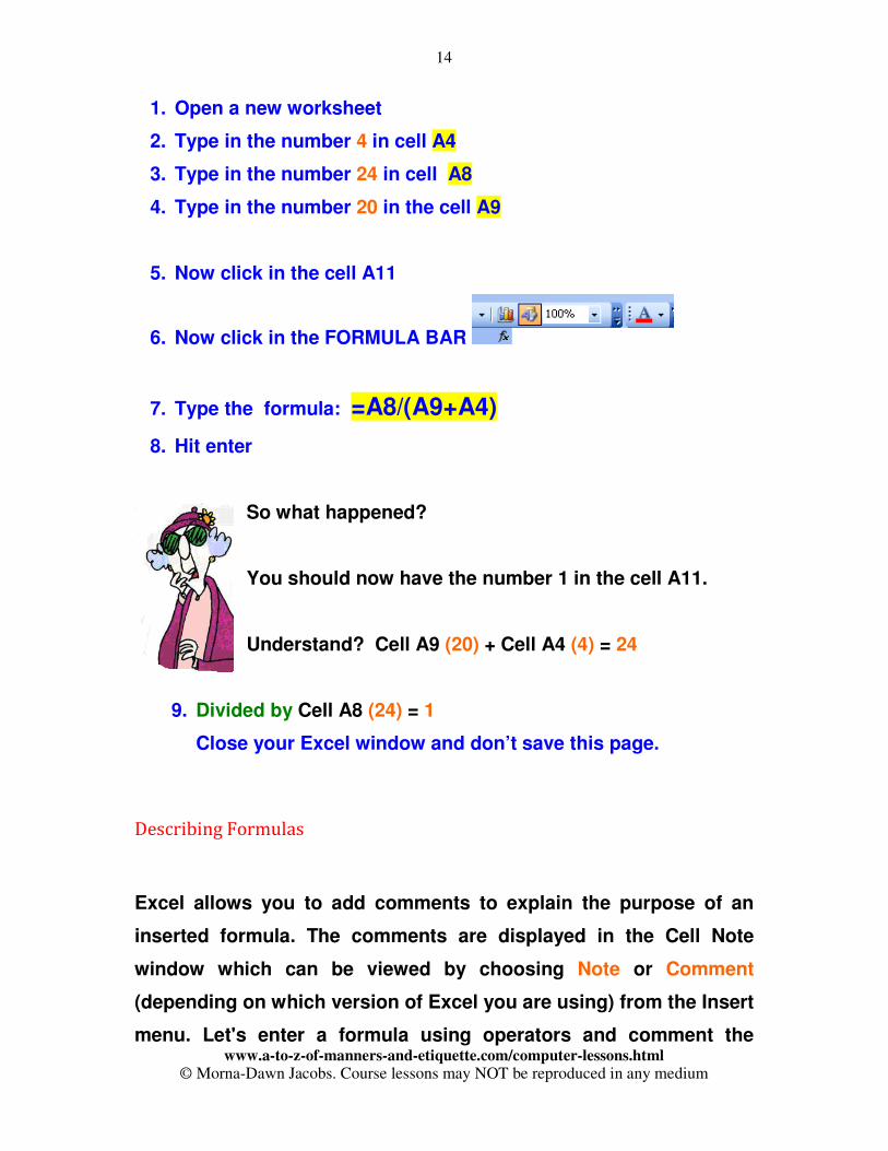
Some familiar operators are: addition (+), subtraction (-), multiplication (*), and division (/). There is an order of operations when you are evaluating a formula. (stay with me … ) Formulas are evaluated from left to right, with expressions enclosed in parentheses evaluated first, then exponents, multiplication, division, addition, and subtraction. (I know that’s a mouthful!! Just carry on – it will make sense later on). Excel has many more operators, but we will work with the operators listed above for now. Here is an example of how the order of operations works: If you have the following formula within a cell; =A8/(A9+A4) The first operation would be the sum of A9 and A4 and then A8 would be divided by that sum. Go ahead, try it out.
14
www.a-to-z-of-manners-and-etiquette.com/computer-lessons.html
© Morna-Dawn Jacobs. Course lessons may NOT be reproduced in any medium
1. Open a new worksheet
2. Type in the number 4 in cell A4
3. Type in the number 24 in cell A8
4. Type in the number 20 in the cell A9
5. Now click in the cell A11
6. Now click in the FORMULA BAR
7. Type the formula: =A8/(A9+A4)
8. Hit enter
So what happened?
You should now have the number 1 in the cell A11.
Understand? Cell A9 (20) + Cell A4 (4) = 24
9. Divided by Cell A8 (24) = 1
Close your Excel window and don’t save this page.
Describing Formulas
Excel allows you to add comments to explain the purpose of an
inserted formula. The comments are displayed in the Cell Note
window which can be viewed by choosing Note or Comment
(depending on which version of Excel you are using) from the Insert
menu. Let's enter a formula using operators and comment the
15
www.a-to-z-of-manners-and-etiquette.com/computer-lessons.html
© Morna-Dawn Jacobs. Course lessons may NOT be reproduced in any medium
formula.
Open a new workbook window.
1. Starting in cell A1 build the following table:
You are going to enter a formula which will calculate the
average of these nine grades.
2. Select cell A11 and type in the text: Total.
It would be best if the total sum of the grades was beneath the last
grade. You need to insert a column between column A and column
B so you don't have to retype all the numbers.
Insert a Column
3. Highlight column A by clicking in the column heading.
Observe:
16
www.a-to-z-of-manners-and-etiquette.com/computer-lessons.html
© Morna-Dawn Jacobs. Course lessons may NOT be reproduced in any medium
4. Choose Columns from the Insert
menu.
Column A should be a blank column now.
Select cell B1 and click in the formula bar.
Highlight the text: Grades and Cut and Paste the
text into cell A1.
Cut and Paste the text: Total into cell A11.
Now to enter the formula for the total sum of the
grades.
Select cell B11 and enter the following formula:
Remember to click on the Enter button or press the Return key
to enter the formula.
Your worksheet should look as follows:
5. Select cell A12 and enter the text: Average.
Select cell B12 and enter the following formula:
17
www.a-to-z-of-manners-and-etiquette.com/computer-lessons.html
© Morna-Dawn Jacobs. Course lessons may NOT be reproduced in any medium
Your worksheet should look as follows:
Let's annotate (comment) the formula in cell B12.
Annotating Formulas
You can attach notes to cells by using comments, formerly called
cell notes.
You can view each comment when you rest the pointer over the cell
or view all comments at the same time. You can print comments in
the same locations where they are displayed on the worksheet or a
list at the end of the worksheet.
Microsoft Excel uses the user's name in each comment.
1. Select cell B12.
2. Choose Comment from the Insert menu.
The following Cell Comment box should appear:
18
www.a-to-z-of-manners-and-etiquette.com/computer-lessons.html
© Morna-Dawn Jacobs. Course lessons may NOT be reproduced in any medium
Within the Text Note box, type in the text: Average of nine grades
and then click anywhere outside the box.
Note that there is a red note indicator in the upper- right corner of
the cell. Anytime you put the mouse over the red note indicator,
your comment will appear.
Now that you know how to compute the average using operators, it
is time to learn how to write a formula using Excel's functions.
Functions
Functions are used to form all or part of a formula. Excel provides
two general types of mathematical functions: those that are used in
business applications and those that are oriented to higher
mathematics. In this tutorial we will focus on the business
applications formulas.
The AutoSum button ( ) located in the Standard toolbar.
Whenever you click the AutoSum button, Excel inserts a SUM()
function in the active cell. Not only will the SUM() function write the
sum formula, but it will make a guess at what range of cells you
19
www.a-to-z-of-manners-and-etiquette.com/computer-lessons.html
© Morna-Dawn Jacobs. Course lessons may NOT be reproduced in any medium
desire to sum, and will leave you in edit mode so that you can
correct the sum range.
1. Select cell C11 and click on the AutoSum button located
in the Standard toolbar.
Your worksheet should look as follows:
Excel has guessed that you want to insert cell B11, which contains
the appropriate formula. Let's assume Excel did not guess
correctly.
2. Within the formula bar highlight B11 and delete it.
The Sum function is waiting for it's arguments.
You want to sum up B2 through B10, this is denoted in a more
compact form as B2:B10.
3. Position your cursor in the formula bar, cut out B11 and
instead type in B2:B10.
4. Observe:
20
www.a-to-z-of-manners-and-etiquette.com/computer-lessons.html
© Morna-Dawn Jacobs. Course lessons may NOT be reproduced in any medium
Click on the Enter button or
press the Return key to enter
the formula.
The Sum function is one of the
many functions Excel provides.
Excel also provides many
statistical functions in particular the Average function.
Excel provides two ways for entering function names. You can type
in the name of the function if you know it or you can use the
Function Wizard.
Using The Function Wizard
To use the Function Wizard you can choose Function from the
Insert menu or you can click on the Function Wizard button ( )
located on the Standard toolbar.
Select cell C12 and open the Function Wizard dialog box by either
method described above.
Observe:
21
www.a-to-z-of-manners-and-etiquette.com/computer-lessons.html
© Morna-Dawn Jacobs. Course lessons may NOT be reproduced in any medium
We want to use the AVERAGE function. The AVERAGE function will
take the average of all the numbers you list in the parentheses. The
Function Wizard will take you through setting up the formula step
by step.
Within the Function Wizard dialog box highlight the Function
Category: Most Recently Used and highlight the Function Name:
AVERAGE then click on the OK button.
The following dialog box should appear:
22
www.a-to-z-of-manners-and-etiquette.com/computer-lessons.html
© Morna-Dawn Jacobs. Course lessons may NOT be reproduced in any medium
Enter the range B2:B10 and then click on the OK button.
Click on the Enter button or press the Return key to enter the
formula.
Your workbook should look as follows:
Now that you know how to enter formulas using operators and
functions, you can practice on your "cheques" workbook.
1. Close Workbook3 and don't save the file.
2. Open the "cheques" workbook.
3. Select cell F3 and enter the following formula:
This formula will compute your balance after cheque 100 has been
written.
4. Select cell F4 and enter the
following formula:
This formula will compute your
balance after cheque 101 has been
written.
23
www.a-to-z-of-manners-and-etiquette.com/computer-lessons.html
© Morna-Dawn Jacobs. Course lessons may NOT be reproduced in any medium
5. Select cell F5 and enter the following formula:
This formula will compute your balance after cheque 102 has been
written plus the $900 dollar deposit has been accounted for.
6. Select cell F6 and enter the formula that would compute the
balance after 103 has been written.
Your "cheques" workbook should look as follows:
If something is incorrect in your "cheques" workbook, go back and
check over your formulas.
7. Save your changes.
8. Starting in cell B3, build the following table:
24
www.a-to-z-of-manners-and-etiquette.com/computer-lessons.html
© Morna-Dawn Jacobs. Course lessons may NOT be reproduced in any medium
You will learn how to format the dates, headings, and dollar
amounts in the next part of the tutorial.
Formatting The Appearance of a Workbook
You will learn how to format an Excel workbook in this part of the tutorial. 1. Open your "cheques" workbook if it isn't already opened. 2. Select the first row of the "cheques" workbook, by clicking in the cell containing the bold face 1. Observe:
You have just selected what Excel describes as a range.
The Concept of a Range
A range is a rectangular block of cells. Many things are
accomplished in Excel using ranges. For instance, the format used
to display values can be changed for an entire range. All the values
in a range can be referred to when writing a formula. A range of
25
www.a-to-z-of-manners-and-etiquette.com/computer-lessons.html
© Morna-Dawn Jacobs. Course lessons may NOT be reproduced in any medium
cells can also be protected, which means the contents of the cells
cannot be altered. Ranges can also be named.
Excel also allows you to select discontinuous ranges. You will learn
how to do this further on in the tutorial.
3. With the range of cells A1:F1 selected, click on the Bold button
and Center alignment button.
This formatting should have made the text too big for the cells.
4. Adjust the column widths of the columns.
Your workbook should look similar to the following:
Selecting Discontinuous Ranges
5. Select the first range of cells: A3:A6. 6. Hold down the Ctrl key and select the range of cells: C2:C6. Observe:
26
www.a-to-z-of-manners-and-etiquette.com/computer-lessons.html
© Morna-Dawn Jacobs. Course lessons may NOT be reproduced in any medium
7. Click on the Center alignment button. The items get centered. 8. Now let's format the dates.
Formatting Dates and Numbers
The basic formatting rule "select and then do" is used when working with Excel. 9. Select the range of cells: B3:B6. 10. Choose Cells from the Format menu. The following Format Cells dialog box should appear:
11. Click on the Number tag if it is not already displayed. 12. Within the Category box highlight Date to view all the Format Codes. 13. Scroll through the options in the Format Codes. There is no format that displays as: Aug. 8,
27
www.a-to-z-of-manners-and-etiquette.com/computer-lessons.html
© Morna-Dawn Jacobs. Course lessons may NOT be reproduced in any medium
96. You can custom format by typing in the Code box. 14. Within the Code box, type in the following custom format:
15. Click on the Center alignment button to align the dates. Now let's format the dollar amounts. 16. Select the discontinuous range displayed below:
Remember to select the first region and then hold down the Ctrl key when you select the remaining regions. 17. Choose Cells from the Format menu. 18. Click on the Number tab if it is not already displayed. 19. Within the Category box highlight Currency. 20. Select the following Format Code and then click OK:
28
www.a-to-z-of-manners-and-etiquette.com/computer-lessons.html
© Morna-Dawn Jacobs. Course lessons may NOT be reproduced in any medium
21. Click on the Center alignment button to align the dollar amounts. Note that you could have selected the whole "cheques" workbook and then clicked on the Center button. Your "cheques" workbook should look as follows:
Let's insert a row between row 2 and row 3 in the "cheques" workbook, to make the workbook more appealing to the eye. 22. Select row 3 by clicking on the bold face 3.
29
www.a-to-z-of-manners-and-etiquette.com/computer-lessons.html
© Morna-Dawn Jacobs. Course lessons may NOT be reproduced in any medium
23. Choose Rows from the Insert menu. You have now learned how to format an Excel document. Note that within the Format Cells dialog box you can format the borders of the cells, change the color, pattern, and shading of the cells and protection of cells can be set there too. You have completed your first workbook. It is time to preview it. 24. Choose Print Preview from the File menu. Observe:
25. Click on the Close button to return you to the workbook. Observe the dotted line between column E and column F, the dotted line indicates that there will be a page break there. What you want to do is actually flip the table so it will fit on the whole page. You can do this by choosing Page Setup from the File menu. 26. Choose Page Setup from the File menu. The following Page Setup dialog should appear:
30
www.a-to-z-of-manners-and-etiquette.com/computer-lessons.html
© Morna-Dawn Jacobs. Course lessons may NOT be reproduced in any medium
27. Click on the Page tab if it isn't already displayed. 28. Within the Orientation box click on Landscape and then click on the OK button. 29. Observe the dotted line (indicating a page break) at the bottom of your workbook and running horizontal. 30. Preview your "cheques" workbook and then print a copy of it. 31. When you are done printing close the "cheques" workbook.
You are now ready to learn some
advanced features
Advanced Excel (Copying Cells)
31
www.a-to-z-of-manners-and-etiquette.com/computer-lessons.html
© Morna-Dawn Jacobs. Course lessons may NOT be reproduced in any medium
In this part of the tutorial you will be creating a workbook and
learning how to fill a cell or range of cells with formulas to speed
data entry.
1. Find and Open Excel if it isn't already open.
2. Choose New from the File menu to start a new workbook if
there isn't a new workbook open.
3. Choose Formula Bar from the View menu to display the formula
bar.
You will be creating an income
statement worksheet.
Make the entries displayed on the
left:
32
www.a-to-z-of-manners-and-etiquette.com/computer-lessons.html
© Morna-Dawn Jacobs. Course lessons may NOT be reproduced in any medium
4. Select the text below the bold faced headings, and right justify
the text.
Remember to hold down the Ctrl
key when selecting a discontinuous
(irregular) range.
Observe:
Your workbook should look as follows:
33
www.a-to-z-of-manners-and-etiquette.com/computer-lessons.html
© Morna-Dawn Jacobs. Course lessons may NOT be reproduced in any medium
5. Before you enter any formulas, let's name some of the cells in
your worksheet.
Naming Cells
Excel allows you to name any cell, range, or value in a workbook.
You can then use this name to refer to the cell, range, or value.
Names make formulas easier to read, understand, and maintain.
You can change or delete names that have been defined previously.
Names appear in the reference area of the formula bar when you
select a named cell or range.
6. Select cell B6 and choose Name from the Insert menu, and
choose Define from the Name submenu.
7. Within the Names dialog box, Excel provides a possible name:
Sales. This is fine. Click the OK button.
8. Select cell B7 and name it: Service.
9. Enter the following constants into your workbook:
10. Select cell B8 and enter the formula
that sums Sales and Services.
11. Save your workbook as "company".
The formula in cell B8 should be either
the formula =B6+B7 or =SUM(B6:B7).
34
www.a-to-z-of-manners-and-etiquette.com/computer-lessons.html
© Morna-Dawn Jacobs. Course lessons may NOT be reproduced in any medium
The formula is summing up the two cells directly above cell B8. If
you look at cell B13, it will need a formula too.
The formula in cell B13 will also sum up the two cells directly above
it.
This is where Excel's Copy command is useful. What you can do is
copy the formula from one cell to another cell.
Copying From One Cell to Another Cell
1. Select cell B8.
2. Choose Copy from the Edit menu.
3. Excel places a marquee around the cell.
4. Select cell B13 and choose Paste from the Edit menu.
Your company workbook should look as follows:
5. Press the Escape key on
your keyboard to cancel
the marquee.
Select cell B13. The
formula should be
=B11+B12 or
=SUM(B11:B12). That is
the formula has
summed the two cells
directly above cell B13.
Your company workbook should look as follows:
35
www.a-to-z-of-manners-and-etiquette.com/computer-lessons.html
© Morna-Dawn Jacobs. Course lessons may NOT be reproduced in any medium
6. Save your work before proceeding.
You now know how to copy a formula from one cell to another.
Next, in order to duplicate the Qtr. heading across columns C
through E, you will make a copy from one cell to several other cells.
Copying From One Cell to Several Cells
1. Select cell B4 and choose Copy from the Edit menu.
2. Highlight the range C4:E4.
3. Choose Paste from the Edit menu.
4. Press the Escape key to remove the marquee.
Your company workbook should look as follows:
36
www.a-to-z-of-manners-and-etiquette.com/computer-lessons.html
© Morna-Dawn Jacobs. Course lessons may NOT be reproduced in any medium
Center the Qtr.
headings.
5. Save your
work before
proceeding.
The next step is to
fill in the range
C6:E7 with
projected
revenues.
6. Select cell C6
and enter the formula =B6*1.08 (assume 8% growth per
quarter).
7. Choose Copy from the Edit menu.
8. Highlight the range C6:E7.
9. Observe:
10. Choose Paste from the Edit menu.
Your
company
workbook
37
www.a-to-z-of-manners-and-etiquette.com/computer-lessons.html
© Morna-Dawn Jacobs. Course lessons may NOT be reproduced in any medium
should look as follows:
11. Highlight the cells in the range C6:E7 and observe the cell's
formulas. In each cell the formula multiplies the cell directly to
the left of it by 1.08.
You can also copy data and formulas from one location on the
workbook to another using the Fill command.
The Fill Command.
1. Select the range B8:E8.
2. Choose Fill from the Edit menu, and from the Fill submenu
choose Right.
Your company workbook should look as follows:
3. The projected expenses in the range C11:E12 are computed as
1.02 times the value of the previous quarter.
38
www.a-to-z-of-manners-and-etiquette.com/computer-lessons.html
© Morna-Dawn Jacobs. Course lessons may NOT be reproduced in any medium
4. Select cell C11 and enter the formula =B11*1.02(assume 2%
growth per quarter).
5. Select the range C11:C13 and choose Fill from the Edit menu,
and from the Fill submenu choose Down.
Your company workbook should look as follows:
Excel also provides another means of copying text, values, or
formulas from one cell to other cells. Excel provides the AutoFill
command. AutoFill copies cell's contents with out using the menu.
You work directly on the workbook using the mouse.
Copying Cells Using AutoFill The AutoFill feature is used to copy formatting, formulas, or all cell
contents, or to perform different types of series extensions. For
example, if you type Monday and Tuesday in consecutive columns,
39
www.a-to-z-of-manners-and-etiquette.com/computer-lessons.html
© Morna-Dawn Jacobs. Course lessons may NOT be reproduced in any medium
and then drag the fill handle to the right, Excel fills Wednesday,
Thursday and so on into selected cells.
1. Select cell C11. Cell C11 contains the formula you want to copy.
2. Observe the fill handle located in the lower
right corner of C11.
3. Place your mouse over the fill handle (black square dot in the
lower right corner of C11), until the arrow
becomes a black cross.
4. Drag the fill handle across the cells D11 and E11 and then
release the mouse button. The formula in C11 gets copied to
D11 and E11.
5. Your company workbook should look as follows:
You can also select more than one cell and then use the AutoFill
command to copy.
1. Select the range C12:C13.
2. Drag the fill handle across the range D12:E13.
40
www.a-to-z-of-manners-and-etiquette.com/computer-lessons.html
© Morna-Dawn Jacobs. Course lessons may NOT be reproduced in any medium
Your company workbook should look as follows:
You have now learned how to copy in Excel. You may use any
method above to finish the company workbook.
1. Select cell B16 and enter the formula =B8-B13. (Gross Income
is equal to Total Revenue minus Total Expenses)
2. Select cell B17 and enter the formula =B16*.22. (The Tax is 22%)
3. Select cell B18 and enter the formula =B16-B17.
(Net Income is Gross Income minus
the Tax)
Enough enough …. !!!!!
Only a little bit more then you can
relax … (smile)
41
www.a-to-z-of-manners-and-etiquette.com/computer-lessons.html
© Morna-Dawn Jacobs. Course lessons may NOT be reproduced in any medium
Your company workbook should look as follows:
4.
Copy the formulas in the range B16:B18 to the range C16:E18
using any method you would like.
Your company workbook should look as follows:
You have almost completed your company workbook. There is one
more column to enter.
42
www.a-to-z-of-manners-and-etiquette.com/computer-lessons.html
© Morna-Dawn Jacobs. Course lessons may NOT be reproduced in any medium
5. Select cell F4 and enter and center the text: Year.
6. Select cell F6 and enter the formula =SUM(B6:E6).
7. Copy the formula in cell F6 into the following ranges: F7:F8,
F11:F13, and F16:F18.
Your completed company workbook should look as follows:
8.
Save your changes.
Close your computer, go down to the beach
for while and come back tomorrow to finish
this (smile)… There’s about another 26
pages to learn …. I’ll leave it up to you.
Your company workbook is complete. You
can now use the power of Excel's automatic
recalculation feature. You can now use What If? analysis.
43
www.a-to-z-of-manners-and-etiquette.com/computer-lessons.html
© Morna-Dawn Jacobs. Course lessons may NOT be reproduced in any medium
What If? Analysis
What If? analysis involves three steps:
1. First, you ask a What If? question about your workbook. For
example, "What if the sales revenue in the first quarter was
$5,000?"
2. Second, you alter the appropriate cell or cells in your
workbook. In this case it would be cell B6.
3. Third, you observe how the different values in the workbook
change.
Experiment with a What If? analysis and enter $5,000 into cell B6.
1. Observe that the Income entries are now negative.
2. Undo the entering of $5,000 or enter $101,000 in cell B6.
Now that you are done with your company workbook, you can learn one more of Excel's advanced features: Linking.
Linking Documents in Excel
Excel can dynamically link a workbook to source data in another
workbook so that any changes you make in one workbook are
immediately reflected in the other workbook.
The following terms apply to linking documents:
• External Reference- A reference to another Excel workbook cell, cell range, or defined name. A formula containing an external reference is called an external reference formula.
44
www.a-to-z-of-manners-and-etiquette.com/computer-lessons.html
© Morna-Dawn Jacobs. Course lessons may NOT be reproduced in any medium
• Dependent Workbook- A workbook that contains a link to another workbook. In other words, a workbook that relies on information in another workbook.
• Source Workbook- A workbook that is the source of the information referred to in an external reference formula; source workbooks are referred to by dependent workbooks.
Creating Links between workbooks
You will need two workbooks to create a link.
The company workbook will serve as your first and as the Source
Workbook.
The second workbook will be created and serve as the Dependent
Workbook.
1. Let's start by creating the Dependent Workbook.
2. Choose New from the File menu to start a new workbook.
3. Create the following workbook and call it Personal Budget:
4. Select cell C6
and enter the
formula
=C4+C5.
5. Select cell C11
and enter the
formula
=C9+C10.
6. Select C13 and enter the formula =C6-C11.
45
www.a-to-z-of-manners-and-etiquette.com/computer-lessons.html
© Morna-Dawn Jacobs. Course lessons may NOT be reproduced in any medium
Your budget workbook should look as follows:
It is now time to create a link between the workbooks; company
and budget.
7. Have both workbooks open.
8. In the Source Workbook: company select cell F18.
This is the cell you want to refer. You want to insert this value
into your budget workbook.
9. Click the Copy button or choose Copy from the Edit menu.
10. A moving border should appear around cell F18.
11. Switch to the budget workbook.
12. This is the workbook you want to paste the linked data.
13. Select cell C4.
14. This is the cell in which you want the linked data to appear.
15. Choose Paste Special from the Edit menu.
46
www.a-to-z-of-manners-and-etiquette.com/computer-lessons.html
© Morna-Dawn Jacobs. Course lessons may NOT be reproduced in any medium
16. The following Paste Special dialog box should appear:
17. Choose All in the Paste box and None in the Operation box.
18. Choose the Paste Link button to paste the link into cell C4.
Your budget workbook should look as follows:
Excel created an external
reference formula that links
the workbooks. This formula
appears in the formula bar.
You have successfully linked two documents. You can now play
around with What If? analysis and see how changes in the Book
Company's income will effect your personal budget.
19. Save your changes.
One of Excel's major features is its ability to produce charts that
illustrate the numbers on the worksheets you produce. In the last
47
www.a-to-z-of-manners-and-etiquette.com/computer-lessons.html
© Morna-Dawn Jacobs. Course lessons may NOT be reproduced in any medium
part of the tutorial you will learn the creation, formatting, and
printing of charts.
Creating Charts
Before you can draw a chart using Excel, the numbers that compose the chart must be entered in a workbook. There are five general steps in defining a chart. Steps in Creating a Chart:
1. Enter the numbers into a workbook.
2. Select the data to be charted.
3. Choose Chart from the Insert menu.
4. Choose either Chart Type from the Format menu or click on the ChartWizard button.
5. Define parameters such as titles, scaling color, patterns, and legend.
These five steps should be performed in this order. Note that since
the chart is linked to the workbook data, any subsequent changes
made to the workbook are automatically reflected in the chart.
You will be making two charts in this part of the tutorial. The first
chart will be a pie chart and the second chart will be a column
chart.
Creating a Pie Chart
Pie charts are used to show relative proportions of the whole, for
48
www.a-to-z-of-manners-and-etiquette.com/computer-lessons.html
© Morna-Dawn Jacobs. Course lessons may NOT be reproduced in any medium
one data series only.
Data series are a group of related data points.
A data point is a piece of information that consists of a category
and value.
For example, if you were collecting data on how couples first meet,
then the number of couples who met through friends would be a
data point. In this case the category is "through friends" and the
value is the number of couples who met that way.
When you create a chart with Excel, the categories are plotted
along the horizontal or X-axis, while the values are plotted along the
vertical or Y-axis.
Data series originate from single worksheet rows or columns. Each
data series in a chart is distinguished by a unique color or pattern.
You can plot one or more data series in a chart except for pie
charts.
An example of a data series is the population of the United States
over ten years. Each data point would be made up of a year (the
category) and the population in that year (value).
The first step in creating any chart is to enter the data on a
workbook.
49
www.a-to-z-of-manners-and-etiquette.com/computer-lessons.html
© Morna-Dawn Jacobs. Course lessons may NOT be reproduced in any medium
1. Find and open Excel if it is not already open.
Make sure your toolbars and formula bar is displayed.
2. Open a new workbook.
3. Save your workbook and name it "expenses".
4. Enter the following into your expenses workbook:
You will be using the ChartWizard to create your pie chart.
Using The ChartWizard
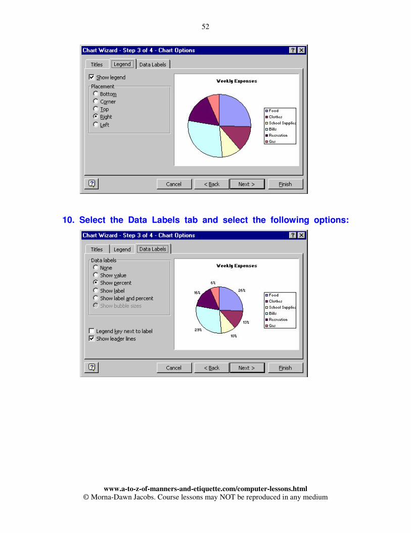
The ChartWizard is a series of dialog boxes that guide you through the steps required to create a new chart or modify settings for an existing chart. When creating a chart with the ChartWizard, you can specify the worksheet range, select a chart type and format, and specify how you want your data to be plotted. You can also add a legend, a chart title, and a title to each axis.
50
www.a-to-z-of-manners-and-etiquette.com/computer-lessons.html
© Morna-Dawn Jacobs. Course lessons may NOT be reproduced in any medium
There are two commands and two buttons that start the ChartWizard. The command you choose or the button you click will create either an embedded chart or a chart sheet. An embedded chart is a chart object that has been placed on a worksheet and that is saved on that worksheet when the workbook is saved. When it is selected you can move and size it. When it is activated, you can select items and add data, and format, move, and size items in the chart. A chart sheet is a sheet in a workbook containing a chart. When a chart sheet is created, it is automatically inserted into the workbook to the left of the worksheet it is based on. When a chart sheet is activated, you can select items and add data, and format, move and size items in the chart. In this tutorial you will be creating chart sheets only. 1. Select the data you just entered.
2. Choose Chart from the Insert menu.
3. Observe that the ChartWizard's first dialog box appears:
51
www.a-to-z-of-manners-and-etiquette.com/computer-lessons.html
© Morna-Dawn Jacobs. Course lessons may NOT be reproduced in any medium
4. You want a regular pie chart not a 3-D pie chart.
5. Select the chart type: Pie and click on the Next button.
The following dialog should
appear:
6. Read the dialog box, make
sure the range is correct and
then click the Next button.
7. The following dialog should
appear:
8. Select the Titles tab and then enter "Weekly Expenses" as the
chart title.
9. Select the Legend tab and make the following adjustments:
52
www.a-to-z-of-manners-and-etiquette.com/computer-lessons.html
© Morna-Dawn Jacobs. Course lessons may NOT be reproduced in any medium
10. Select the Data Labels tab and select the following options:
53
www.a-to-z-of-manners-and-etiquette.com/computer-lessons.html
© Morna-Dawn Jacobs. Course lessons may NOT be reproduced in any medium
11. Select the following options and then click the Finish button.
Your expenses workbook should look as follows:
12. Save your changes.
54
www.a-to-z-of-manners-and-etiquette.com/computer-lessons.html
© Morna-Dawn Jacobs. Course lessons may NOT be reproduced in any medium
Once you complete the ChartWizard, Excel displays the new chart
sheet, the Chart toolbar ( ),
and the chart menu bar. Note that if the chart toolbar is not
displayed, simply choose Toolbars from the View menu and check
of the chart box. The chart menu bar is similar to the worksheet
menu bar, except the Insert and Format menus have some different
commands.
Now that the initial chart is created, it is time to learn how to format
it.
Formatting a Chart
Before we can discuss the details of how to edit and format a chart, you need to know how to activate the chart and select items in the chart using a mouse.
Activating a Chart Sheet
When you activate a chart, the chart menu commands become
available and the Chart toolbar is displayed.
To activate a chart sheet, select the chart sheet tab you want.
Select the chart sheet tab to activate the pie chart.
55
www.a-to-z-of-manners-and-etiquette.com/computer-lessons.html
© Morna-Dawn Jacobs. Course lessons may NOT be reproduced in any medium
Once a chart is active, you can use the mouse to select chart items
one at a time. To confirm what you have selected, refer to the name
box on the formula bar.
Note that many items in a chart are grouped together. For some
grouped items, such as data series, you click once to select the
entire group, and then click the individual item you want to select
within the group. The following list is a brief overview on how to
select items in a chart using a mouse.
Selecting Items In a Chart Using a Mouse
To select one of the following items in an Excel chart:
• Data Series- click any data marker belonging to a data series.
• Pie slice- select the pie ring, and then click the slice.
• Data labels- click any data label associated with a data series.
• Single data label- select the data labels, and then click an
individual label.
• Legend- click anywhere in the legend, or click its border.
• Single legend entry- select the legend, and then click the
legend entry.
• Title- click the chart title, axis title, or text box.
56
www.a-to-z-of-manners-and-etiquette.com/computer-lessons.html
© Morna-Dawn Jacobs. Course lessons may NOT be reproduced in any medium
• Axis- click the axis or a tick-mark label to format or modify the
axis.
Let's change the colors of
the pie slices.
1. Select the Pie ring.
2. Your pie chart should
look similar to the
following:
3. Select the 29% pie slice.
57
www.a-to-z-of-manners-and-etiquette.com/computer-lessons.html
© Morna-Dawn Jacobs. Course lessons may NOT be reproduced in any medium
Observe:
58
www.a-to-z-of-manners-and-etiquette.com/computer-lessons.html
© Morna-Dawn Jacobs. Course lessons may NOT be reproduced in any medium
4. Choose Selected Data Point from the Format menu.
The following Format Data Point dialog box should appear:
5. Select the Patterns tab and choose a different color and pattern
for the slice.
6. Select another pie slice and change its color.
7. Select the Chart title.
Observe:
8.Choose a different
color from the Font
59
www.a-to-z-of-manners-and-etiquette.com/computer-lessons.html
© Morna-Dawn Jacobs. Course lessons may NOT be reproduced in any medium
Color button ( ).
9. Select the chart.
Observe the ChartWizard toolbar that is displayed on your screen.
There is a Legend button located on the toolbar. If you want to add
or delete a legend to a chart just press that button.
Now that you have completed your weekly expenses pie chart let's
print it out. Before you print it out let's preview it.
10. Save all your changes.
11. Choose Print Preview from the File menu.
Make sure that the text: Page 1 and Chart 1 is not displayed, if this
text appears the layout of the page must be set.
12. Click on the Close button.
13. Choose Page Setup from the File menu.
14. Within the Page Setup dialog box select the Header/Footer tab.
Observe:
15. Within the Header
/Footer box select
(none) from the Header
and Footer pull-down
menus
60
www.a-to-z-of-manners-and-etiquette.com/computer-lessons.html
© Morna-Dawn Jacobs. Course lessons may NOT be reproduced in any medium
61
www.a-to-z-of-manners-and-etiquette.com/computer-lessons.html
© Morna-Dawn Jacobs. Course lessons may NOT be reproduced in any medium
This will clear the text: Chart 1 at the top of your pie chart and it will
also clear the text: Page 1 at the bottom of your pie chart.
16. Within the Page Setup dialog box, select the Chart tab and
select the following setting:
17. Click on the OK button.
18. Click on the Print button.
You are now ready to create a column chart.
62
www.a-to-z-of-manners-and-etiquette.com/computer-lessons.html
© Morna-Dawn Jacobs. Course lessons may NOT be reproduced in any medium
Creating a Column Chart
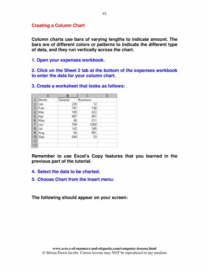
Column charts use bars of varying lengths to indicate amount. The bars are of different colors or patterns to indicate the different type of data, and they run vertically across the chart. 1. Open your expenses workbook. 2. Click on the Sheet 2 tab at the bottom of the expenses workbook to enter the data for your column chart. 3. Create a worksheet that looks as follows:
Remember to use Excel's Copy features that you learned in the previous part of the tutorial. 4. Select the data to be charted.
5. Choose Chart from the Insert menu.
The following should appear on your screen:
63
www.a-to-z-of-manners-and-etiquette.com/computer-lessons.html
© Morna-Dawn Jacobs. Course lessons may NOT be reproduced in any medium
Choose the chart type: Column and click on the Next button. Choose the following format type
and click on the Next button. The following should appear on your screen:
64
www.a-to-z-of-manners-and-etiquette.com/computer-lessons.html
© Morna-Dawn Jacobs. Course lessons may NOT be reproduced in any medium
If the range is correct, click on the Next button. Insert the following on the titles tab and click the Next button. Observe:
6.Select the following options and click the Finish button. Observe:
65
www.a-to-z-of-manners-and-etiquette.com/computer-lessons.html
© Morna-Dawn Jacobs. Course lessons may NOT be reproduced in any medium
Your column chart should look as follows:
Let's format the column chart.
1. Select the business (data series) columns and make them yellow.
66
www.a-to-z-of-manners-and-etiquette.com/computer-lessons.html
© Morna-Dawn Jacobs. Course lessons may NOT be reproduced in any medium
2. Select the general (data series) columns and make them green. Your column chart should look similar to the following:
3. Select a grid line and choose Selected Gridlines from the Format menu.
67
www.a-to-z-of-manners-and-etiquette.com/computer-lessons.html
© Morna-Dawn Jacobs. Course lessons may NOT be reproduced in any medium
4. The following Format Gridlines dialog should appear:
5. Choose a different style for the line and click the OK button.
6. Lastly, let's change the alignment of the text that makes up the
months.
7. Select the X-axis.
8. Choose Selected Axis from the Format menu.
9. Within the Format Axis dialog box click on the Alignment tab.
10. Select the following
option and click the OK
button.
Observe:
Your column chart should
look similar to the one on
the next page:
68
www.a-to-z-of-manners-and-etiquette.com/computer-lessons.html
© Morna-Dawn Jacobs. Course lessons may NOT be reproduced in any medium
11. Preview your chart.
12. Clear the Chart 2 and Page 1 text in the Header and Footer
respectively using the Page Setup command.
13. Print a copy of your column chart.
Congratulations! You have finished the Excel tutorial
That was a MAJOR learning experience.