A Visual Analysis System for Metabolomics Data

Philip Livengood∗, Ross Maciejewski∗, Wei Chen†, David S. Ebert∗

∗ Purdue University Visualization and Analytics Center† State Key Lab of CAD&CG, Zhejiang University

ABSTRACT

When analyzing metabolomics data, cancer care researchers aresearching for differences between known healthy samples andunhealthy samples. By analyzing and understanding these dif-ferences, researchers hope to identify cancer biomarkers. Inthis work we present a novel system that enables interactivecomparative visualization and analysis of metabolomics data ob-tained by two-dimensional gas chromatography-mass spectrome-try (GCxGC-MS). Our system allows the user to produce, andinteractively explore, visualizations of multiple GCxGC-MS datasets, thereby allowing a user to discover differences and featuresin real time. Our system provides statistical support in the form ofmean and standard deviation calculations to aid users in identify-ing meaningful differences between sample groups. We combinethese with multiform, linked visualizations in order to provide re-searchers with a powerful new tool for GCxGC-MS exploration andbio-marker discovery.

1 INTRODUCTION

In recent years, GCxGC-MS has become an invaluable laboratoryanalysis tool. However, this procedure produces large (gigabytesof data per sample), four dimensional datasets (retention time one,retention time two, mass and intensity). Such data is cumbersome,and researchers must spend time formatting and processing the datain order to remove acquisition artifacts, and quantify and identifychemical compounds [9]. Furthermore, while statistical analysishas played an important role in this work (because of the need toreduce the thousands of acquired spectral features to a more man-ageable size), the large data size, inherent biological variability andmeasurement noise makes the identification of bio-markers throughpurely statistical processes extremely difficult and time consuming.

As such, our work focuses on the development of a visual anal-ysis suite for exploring differences across samples and groups ofsamples. In this work, we have created a system that utilizes a seriesof multiform linked visualizations to enable interactive exploration,filtering and comparison of multiple samples simultaneously. Thisallows users to quickly locate feature similarities and differencesacross samples and drill down into the mass spectrum data for de-tailed analysis. These techniques allow researchers to form and ex-plore hypotheses about sample alignment, acquisition artifacts, and(most importantly) cancer bio-marker sites. For example, Figure 1(top) illustrates a cancerous and non-cancerous data sample visual-ized with total ion count (TIC) images. In this example, differencesbetween the two samples are not obvious, and, once differences arefound, it can be difficult to determine whether or not those differ-ences are meaningful. By using our tools, researchers are able toquickly identify and explore sample differences as seen in Figure 1(bottom).

Our work is being developed in collaboration with analyticalchemists and biology researchers, and is designed to provide aninteractive comparative visual analysis environment for GCxGC-MS data exploration. While this work is similar to previous work

Figure 1: GCxGC-MS data sets rendered as 2D TIC images (top).Our system provides visual analytic tools to help researchers iden-tify meaningful differences (bottom). Here we show a canine cancersample (left) compared with a healthy canine sample (right).

[1, 2, 7] in that we provide linked views that support the interactivevisual exploration of mass spectrometry data, our system providesseveral features not currently available in other GCxGC-MS analy-sis systems:

1. a comparative visualization window that allows multiple sam-ples (and multiple views of individual samples) to be dis-played simultaneously,

2. data exploration tools for exploring mass spectra and filteringand comparing TIC images in real-time,

3. grouping of samples and calculation of group means for com-parison and difference calculation,

4. the application of mean and standard deviation TICs to thecolor-mapping of difference measures,

5. a dynamic color scale adaptation tool for discovering differ-ences in low-intensity peaks.

As automated analysis tools take days to run, our system servesas a front end in order to make the calculation tractable by spec-ifying a region for evaluation. With our tool, users may visualizemultiple samples of GCxGC-MS data, interactively search for sam-ple differences, probe areas of interest to bring up mass spectrumplots, and compare regions where the mass spectra deviate the most.These features provide valuable data analysis for bio-marker dis-covery, and make an excellent complement to existing workflows.

2 GCXGC-MS

In cancer care engineering, researchers collect GCxGC-MS data inorder to search for biomarker differences between cancerous andnon-cancerous samples. In GCxGC-MS, a sample to be analyzed isfirst mixed with a carrier gas that transports it through the machine.The device has two columns through which a sample passes beforebeing analyzed by a mass spectrometer. Different components ofthe sample move through the columns at different rates, resultingin two levels of separation according to how long it takes each ofthe components to move through each of the columns. The massspectrometer gives an additional level of separation as the mixtureis ionized when it exits the second column. This process results ina four-dimensional dataset with two time axes (retention time one(RT1) from the first column and retention time two (RT2) from thesecond column), mass, and intensity.

Up to this point we have referred to mass as one of the dimen-sions of data produced by the mass spectrometer. More correctly,we should be referring to this as the mass-to-charge ratio, desig-nated m/z. A mass spectrometer breaks molecules up into ionizedfragments. It is then able to determine the mass-to-charge ratio byusing the fact that two particles with the same m/z will move in thesame path in a vacuum when subjected to the same electrical andmagnetic fields. A particular chemical compound will have a veryspecific mass spectral signature. The spectral signature of unknowncompounds can be compared to a library of known compounds tohelp identify the compound or its composition. This type of identi-fication can be difficult because different chemical compounds mayhave the same retention times, and thus their spectral peaks mayhave significant overlap, a problem known as co-elution.

GCxGC-MS is marked by its large peak capacity, an order ofmagnitude increase in chemical separation ability [1], and its im-proved speed [3]. However, the data obtained exhibits several com-plexities.Samples must be mixed with a carrier gas as part of the ac-quisition process. This carrier gas shows up in the resulting data set,and can obscure sample peaks of interest. Inconsistencies in sampleamounts will lead to differences in peak intensities. Peak retentiontimes and shapes exhibit slight differences that are uncontrollable,yet are unrelated to actual chemical differences in the samples [1].Data samples exhibit background noise that can vary from sampleto sample, and make accurate peak quantification difficult. Finally,despite the improved separation ability over one-dimensional GC-MS, GCxGC-MS still exhibits some peak overlap due to coelution.

Despite these difficulties, GCxGC-MS is used in a wide array ofapplications, such as quality control, chemical identification, andbiomarker detection. As a result, much research has been done todetermine effective ways to analyze the large amounts of data pro-duced and overcome the previously mentioned pitfalls. Alignmentalgorithms [14], background removal algorithms [8], and com-pound identification [10] are common areas of study. Other re-searchers have worked on identifying potentially significant com-pounds, such as the orthogonal partial least-square (OPLS) ap-proach used by Wiklund et al. [13].

3 RELATED WORK

The thrust of this work is the development and deployment of aninteractive visual analysis tool for analyzing data captured throughthe GCxGC-MS process. Kincaid and Dejgaard [6] developed asystem to explore protein complexes in tandem mass spectrometrydata through modifications to a scatter plot visualization. Jourdan etal. [5] also utilized scatterplot matrices and parallel coordinate plotsas a means of exploring metabonomics data. Work by de Corral andPfister [2] presented a system for the three-dimensional visualiza-tion of Liquid Chromatography - Mass Spectrometry (LCMS) data.The goal of this system was to provide LCMS practitioners with anoverview of their data set and enable them to identify features thatcan vary with mass and time, and this research primarily focused

on rendering speeds of large scale LCMS data. Work by Linsen et

Figure 2: A color mapped height field (left). Using the high contrastoption for height field rendering (right), small peaks and backgroundnoise, which might otherwise be hidden, are easily seen.

al. [7] also focused on LCMS data looking at characteristic pat-terns of isotopes. Their visual exploration tools allowed users toclick on labeled peaks to explore mass spectrum data similar to ourproposed system. However, the key difference lies in the ability ofthe user to compare multiple samples simultaneously through dif-ference mappings and linked views.

Perhaps the closest is the work done by Hollingsworth et al. [1],in which they utilize image processing based techniques based onthe total ion count image. Prior to visualization and comparisoneach image must undergo background removal and peak detection.Once this pre-processing is complete, a difference image is com-puted. This difference can be visualized using tabular data, a 2Dimage, or 3D height field visualization in either grayscale or color.Their main contribution is the calculation of a fuzzy difference thatcompares each pixel value in one image with a small neighborhoodof pixels in the other, rather than doing a pixel-by-pixel compar-ison. This technique helps to reduce the incidental differences inpeak shape and retention time that may still exist even after align-ment. While these techniques represent a good first step, they areill-suited for biomarker detection as they rely solely on images pro-duced from the total ion count data, meaning that peaks of inter-est could easily become obscured. Since only the magnitude ofthe difference is considered, the results obtained can be mislead-ing. Large, yet unimportant differences may be emphasized whilesmall, yet meaningful differences may not be noticeable. Addition-ally, there is only limited user interaction available for exploringpeaks and mass spectra.

4 COMPARATIVE VISUAL ANALYTICS SYSTEM

Our work provides a comparative visual analytics system forGCxGC-MS data. The primary goal is to increase data explorationand analysis in order to help researchers determine meaningful dif-ferences between groups of samples. Finding such differences isthe first step in bio-marker identification. We provide both new andtraditional visualization techniques and couple them with linked,interactive exploration. By incorporating mean and standard devia-tion calculations we are able to visualize the significance of differ-ences in peak intensity rather than merely the magnitude of thosedifferences.

In this section, we first discuss our interactive visualization meth-ods. We describe our scheme for total ion count visualization, massspectrum visualization and the various applied color mapping func-tionalities. We then discuss the linked views and data explorationtools including the area selection tool, mass filtering and TIC lens.

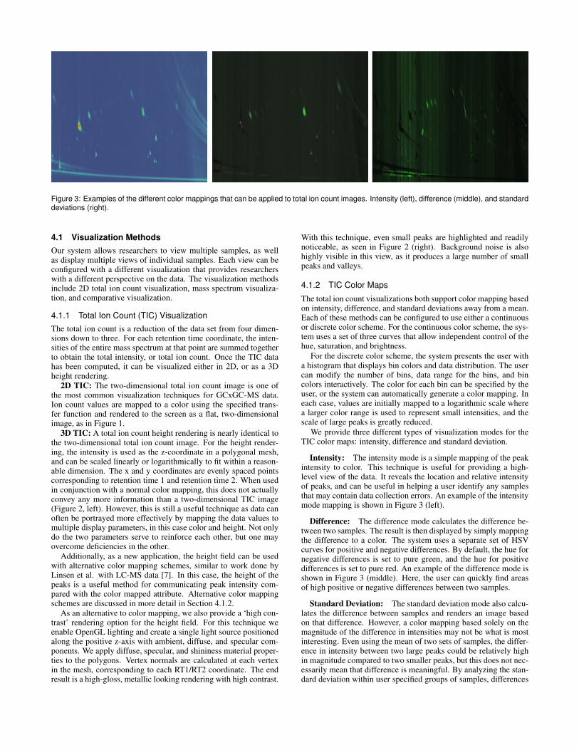
Figure 3: Examples of the different color mappings that can be applied to total ion count images. Intensity (left), difference (middle), and standarddeviations (right).

4.1 Visualization Methods

Our system allows researchers to view multiple samples, as wellas display multiple views of individual samples. Each view can beconfigured with a different visualization that provides researcherswith a different perspective on the data. The visualization methodsinclude 2D total ion count visualization, mass spectrum visualiza-tion, and comparative visualization.

4.1.1 Total Ion Count (TIC) Visualization

The total ion count is a reduction of the data set from four dimen-sions down to three. For each retention time coordinate, the inten-sities of the entire mass spectrum at that point are summed togetherto obtain the total intensity, or total ion count. Once the TIC datahas been computed, it can be visualized either in 2D, or as a 3Dheight rendering.

2D TIC: The two-dimensional total ion count image is one ofthe most common visualization techniques for GCxGC-MS data.Ion count values are mapped to a color using the specified trans-fer function and rendered to the screen as a flat, two-dimensionalimage, as in Figure 1.

3D TIC: A total ion count height rendering is nearly identical tothe two-dimensional total ion count image. For the height render-ing, the intensity is used as the z-coordinate in a polygonal mesh,and can be scaled linearly or logarithmically to fit within a reason-able dimension. The x and y coordinates are evenly spaced pointscorresponding to retention time 1 and retention time 2. When usedin conjunction with a normal color mapping, this does not actuallyconvey any more information than a two-dimensional TIC image(Figure 2, left). However, this is still a useful technique as data canoften be portrayed more effectively by mapping the data values tomultiple display parameters, in this case color and height. Not onlydo the two parameters serve to reinforce each other, but one mayovercome deficiencies in the other.

Additionally, as a new application, the height field can be usedwith alternative color mapping schemes, similar to work done byLinsen et al. with LC-MS data [7]. In this case, the height of thepeaks is a useful method for communicating peak intensity com-pared with the color mapped attribute. Alternative color mappingschemes are discussed in more detail in Section 4.1.2.

As an alternative to color mapping, we also provide a ‘high con-trast’ rendering option for the height field. For this technique weenable OpenGL lighting and create a single light source positionedalong the positive z-axis with ambient, diffuse, and specular com-ponents. We apply diffuse, specular, and shininess material proper-ties to the polygons. Vertex normals are calculated at each vertexin the mesh, corresponding to each RT1/RT2 coordinate. The endresult is a high-gloss, metallic looking rendering with high contrast.

With this technique, even small peaks are highlighted and readilynoticeable, as seen in Figure 2 (right). Background noise is alsohighly visible in this view, as it produces a large number of smallpeaks and valleys.

4.1.2 TIC Color Maps

The total ion count visualizations both support color mapping basedon intensity, difference, and standard deviations away from a mean.Each of these methods can be configured to use either a continuousor discrete color scheme. For the continuous color scheme, the sys-tem uses a set of three curves that allow independent control of thehue, saturation, and brightness.

For the discrete color scheme, the system presents the user witha histogram that displays bin colors and data distribution. The usercan modify the number of bins, data range for the bins, and bincolors interactively. The color for each bin can be specified by theuser, or the system can automatically generate a color mapping. Ineach case, values are initially mapped to a logarithmic scale wherea larger color range is used to represent small intensities, and thescale of large peaks is greatly reduced.

We provide three different types of visualization modes for theTIC color maps: intensity, difference and standard deviation.

Intensity: The intensity mode is a simple mapping of the peakintensity to color. This technique is useful for providing a high-level view of the data. It reveals the location and relative intensityof peaks, and can be useful in helping a user identify any samplesthat may contain data collection errors. An example of the intensitymode mapping is shown in Figure 3 (left).

Difference: The difference mode calculates the difference be-tween two samples. The result is then displayed by simply mappingthe difference to a color. The system uses a separate set of HSVcurves for positive and negative differences. By default, the hue fornegative differences is set to pure green, and the hue for positivedifferences is set to pure red. An example of the difference mode isshown in Figure 3 (middle). Here, the user can quickly find areasof high positive or negative differences between two samples.

Standard Deviation: The standard deviation mode also calcu-lates the difference between samples and renders an image basedon that difference. However, a color mapping based solely on themagnitude of the difference in intensities may not be what is mostinteresting. Even using the mean of two sets of samples, the differ-ence in intensity between two large peaks could be relatively highin magnitude compared to two smaller peaks, but this does not nec-essarily mean that difference is meaningful. By analyzing the stan-dard deviation within user specified groups of samples, differences

can be visualized in more certain terms. We create a standard devia-tion color mapping from a sample group by first calculating a meanTIC for all the samples within that group. Note that the samplesare chosen by the user such that they have been pre-normalized asinput to the system.

Figure 4: The point selection tool is used for comparing TIC values,as well as interactively exploring mass spectra.

Next a standard deviation TIC is calculated as:

σA =

√

1

nA

n

∑i=1

(xi −µA)2 (1)

Here, nA is the number of samples in group A, µA is the mean TICof group A, and the xi are the TICs of the ith sample. Once wehave computed the standard deviation TIC, it is stored to use forcolor mapping. This color mapping can then be applied to a samplevisualization. Generally, it would be applied to a sample that is partof another group. In order to determine the color at a particularretention time coordinate, the system calculates the correspondingz-value for each point b in the new sample, as shown in Equation2. The z-value is simply how many standard deviations different avalue is than the calculated mean. We then use that difference todetermine the appropriate color.

z =µA −b

σA(2)

This can help a user to determine whether an observed differenceis truly meaningful. Additionally, this technique may effectively re-veal areas of difference in smaller peaks that are significant in termsof standard deviations, but were not previously noticed simply be-cause the peaks themselves are smaller. An example is shown inFigure 3 (right), note the green streaks that are not seen in Figure3 (middle). This helps the user explore regions in the image thatare statistically different in a sample when compared to a group ofsamples.

4.1.3 Mass Spectrum Visualization

A mass spectrum view is simply a plot of intensity on the y-axis vs.the mass-to-charge ratio on the x-axis, as seen in Figure 4 (bottom).The user is given the option to plot this spectrum as a bar graph, oras a connected line.

4.2 Linked Views and Data Exploration

Linked views are a common technique for comparative visualiza-tion. This type of interaction aids a user in quickly, and intuitivelyexploring data. Within the context of our system, we provide a

Figure 5: The mass filter tool allows a user to compare specific massvalues using TIC visualizations. In this image, everything exceptmass 100 and 141 have been filtered out for the TIC visualization.

user with multiple tools he may use in order to interact with theviews, including scale, pan, rotate, point selection, area selection,mass filter, and tic lens. Such linked views are not scalable as thenumber of samples to be compared grows; however, by using thedifference and standard deviation views, users can explore sampleswithin groups for comparison, thereby reducing the need for nu-merous side-by-side comparison.

4.2.1 Point Selection

The point selection tool is used on 2D TIC visualizations. Thetool generates point selection messages that can then be handled byother 2D TIC visualization, and by mass spectrum visualizations.As the user interactively moves the cursor over a 2D TIC visualiza-tion, a cursor is displayed at the same location on all 2D TIC vi-sualizations. The total ion count value at that location is displayedin the lower left corner of the window, and mass spectrum viewsare updated with the corresponding mass spectrum at that location,as shown in Figure 4. All of this happens interactively, providingreal-time TIC and mass spectra exploration and comparison for thedata sets.

4.2.2 Area Selection

Rather than selecting a single point, a user may choose to selectan area in a TIC image. This tool allows a user to draw a rectan-gular region on the TIC image. The aggregated TIC value is thendisplayed in the lower left, and mass spectrum visualization are up-dated with the total sum of intensity values for each mass in theentire region. In combination with linked views, this can be used toselect a region containing a specific peak. The total integrated valueof the region can be compared across samples, as well as individ-ual mass values for any spectra that are displayed. The selectedarea can be made large enough so that the peak will be completelywithin the region across all samples, even if there is a slight varia-tion in retention time across some of the samples. This is illustratedin Figures 8 and 9.

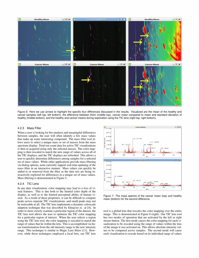
Figure 6: Here we use arrows to highlight the specific four differences discussed in the results. Visualized are the mean of the healthy andcancer samples (left top, left bottom), the difference between them (middle top), cancer mean compared to mean and standard deviation ofhealthy (middle bottom), and the healthy and cancer means during exploration using the TIC lens (right top, right bottom).

4.2.3 Mass Filter

When a user is looking for bio-markers and meaningful differencesbetween samples, the user will often identify a few mass valuesthat make up some interesting compound. The mass filter tool al-lows users to select a unique mass or set of masses from the massspectrum display. Total ion count data for active TIC visualizationsis then re-acquired using only the selected masses. The color map-ping is then rescaled to match the new range of values across all ofthe TIC displays, and the TIC displays are refreshed. This allows auser to quickly determine differences among samples for a selectedset of mass values. While other applications provide mass filteringvia dialog options, none currently support real-time updating of themass filter in an interactive manner. Mass values can quickly beadded to or removed from the filter as the data sets are being in-teractively explored for differences in a unique set of mass values.Mass filtering is demonstrated in Figure 5.

4.2.4 TIC Lens

In any data visualization, color mapping may lead to a loss of vi-sual features. This is due both to the limited color depth of thedisplay, as well as to the limited perceptual ability of human vi-sion. As a result of these properties, it can be difficult to comparepeaks across separate TIC visualizations, and small peaks may notbe noticeable at all. The TIC lens implements a dynamic colorscaleadaption technique that was described by Elmqvist et. al [4]. Inorder to more closely examine a particular region of the dataset, theTIC lens tool allows the user to optimize the TIC color mappingfor a particular region of interest. When the user selects a regionusing the TIC lens tool, the color mapping is rescaled to match therange of values that lie within the lens. This is accomplished via lin-ear transformation from the old intensity range to the new intensityrange. This technique is similar to Magic Lens filters [11]. How-ever, while those techniques employed a local lens, our TIC lens

Figure 7: The mass spectra of the cancer mean (top) and healthymean (bottom) for the second difference.

tool is a global lens that rescales the color mapping over the entireimage. This is demonstrated in Figure 6 (right). Our TIC lens toolhas two modes of operation that are activated by the left or rightmouse button. The first mode causes the color mapping for each vi-sualization to be rescaled using the range of values within the lensof the image it was activated on. This allows absolute intensity val-ues to be compared across samples. The second mode will causeeach visualization to rescale based on its individual range of values

within the lens region. This allows relative intensity values to becompared across samples. Using this tool with the 2D TIC visual-ization, the intensities of peaks can be more accurately compared,and small peaks that may have been previously hidden can be seenand compared.

5 RESULTS

To evaluate the benefits of our system, we have worked with severalbiological and chemical researchers on several datasets. In orderto better illustrate the use of this system, we describe below onesession of our working side-by-side with a GCxGC-MS researcherto analyze one of his data sets. This particular data set consisted ofcanine serum samples. There were five samples each from healthycanines and canines with cancer. No preprocessing was performedon any of these samples.

He created ‘Cancer’ and ‘Healthy’ groups in order to classify thesamples. After averages for the two groups were calculated, he thencalculated the difference of the two averages. In order to get a quickoverview of the data, the researcher first displayed 2D TIC visual-izations of the means and difference side-by-side.In the differenceimage we observed several red peaks that indicated higher intensi-ties in the cancer mean sample. However, there was a bright greenpeak about one-third of the way up on the difference image towardthe left side, as seen in Figure 6 (top middle) labeled as Arrow 1.As this seemed interesting, he then used the region select tool inorder to get a feeling for the relative peak sizes. He created twomore visualizations in order to simultaneously show the mass spec-tra of these peaks for the mean samples. The first thing we noticedwas that the mean of the healthy samples had a much higher back-ground level than the mean of the cancer samples. Unfortunately,this makes comparison using the TIC values problematic. However,individual mass values can still be compared from the mass spec-tra views, and using this we see that the healthy mean sample hasabout twice the intensity of the cancer mean sample for that peak.He next wanted to verify that this difference was consistent. Allten samples were visualized simultaneously using 2D TIC views.This allowed him to verify that this peak was consistently biggerin the healthy samples. We also noticed a single sample amongthe cancer group that had significantly less background level thanthe other samples. This one outlier was responsible for most of thedifference in background levels between the two means, and wastherefore moved into a new group so that it would not be includedin future comparisons between the calculated means.

In order to dig deeper into the differences between the samples,he next created standard deviation color mappings from the healthyand cancer samples. These color mappings indicated that severalpeaks showed higher than normal intensities in the cancer samples.After adjusting the color mapping to highlight only the largest ofthose differences, he chose to investigate one particularly noticeabledifference near the center of the image, which is shown in Figure6 (bottom, middle). After visualizing all of the samples simultane-ously, use of the region select tool showed a consistent differencebetween the two groups. Again, differences in background levelsreduce the accuracy of using the displayed TIC values as differencemeasures, but by visually inspecting the spectra we could see abouta six-fold difference in intensities between the two groups, as seenin Figure 7.

He next began exploring this area by using the TIC lens tool tocompare the two mean samples. He quickly noticed a peak in thecancer sample that barely showed up in the healthy samples, Figure6 (middle) labeled as Arrow 2. Because this peak was small, itis barely noticeable using the standard color mapping. We zoomedinto that area and immediately noticed two peaks in this area, Figure6 (right) labeled as Arrow 3 and 4. The zoom and differences canbe seen in Figure 6 (right). We again visualized all the samplessimultaneously to look for consistency. The first peak (Arrow 3)

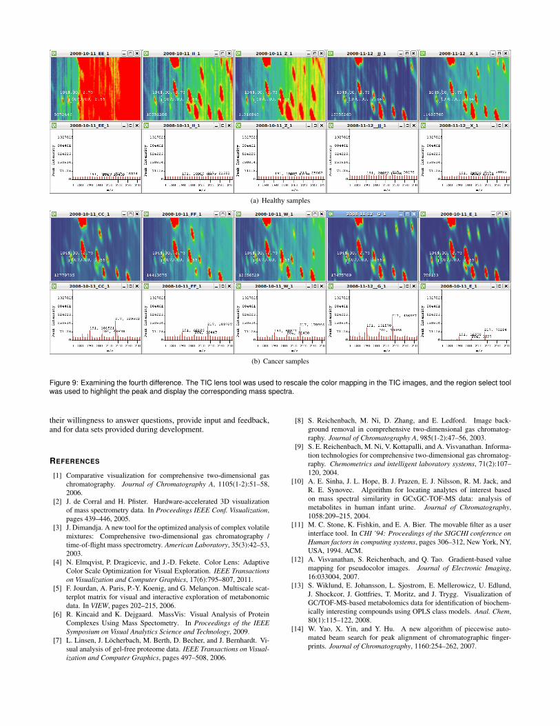
was very prominent in 4 out of the 5 cancer samples. We saw notrace of it in 3 out of 5 healthy samples, and very slight presencein the other 2 healthy samples, as shown in Figure 8. The secondpeak (Arrow 4) was even more consistent, showing a significantpresence in all 5 cancer samples, and little to no presence in all5 healthy samples, as shown in Figure 9. By noting the retentiontime coordinates, he was then able to quickly look up and confirmthese differences using the peak tables generated by commercialsoftware. These consistent differences across samples mean thatthese peaks are potential biomarkers.

6 DISCUSSION

Initial feedback from researchers working with GCxGC-MS datahas been very enthusiastic. This system has provided them withtheir first opportunity to visualize multiple samples simultaneously.Enthusiasm has also been expressed about mean, standard devia-tion, and difference calculation for a set of samples. By visualizingthese calculated data, the human eye can quickly identify differ-ences. This system can be used to identify a particular peak orregion of difference, and then the mass spectra can be explored toprovide validation of differences, and hypotheses about the com-pounds involved. With this information, their existing tools can beused to obtain information about compound identification and in-tensity details much more quickly than was previously possible.

The researchers also frequently mentioned how pleased theywere with the speed of the software. Other commercial systemswill often take tens of seconds or minutes to even display a TICimage. Additionally, these software systems allow masses to be fil-tered, and individual spectra to be visualized, however, it is a slowand cumbersome process to change parameters and redisplay a newspectra or filter out different mass values. No other system cur-rently used by this group was able to provide the fast, interactivefiltering and mass spectra exploration of our system. As an exam-ple, the researchers can now quickly change the mass filter for aspecific value, and slowly move through the entire range of massvalues. Multiple samples can be visualized, and as the mass filter isupdated the researchers can very quickly visually identify cases inwhich a unique mass has an unusual abundance in some samples.Currently, a version of this system is deployed for use on the CancerCare Engineering Hub at Purdue University, http://ccehub.org.

7 CONCLUSIONS AND FUTURE WORK

As our system was evaluated, we also received several suggestionfor future work. Plans for future work involve producing output thatcan be used by other tools. For example, we could allow the userto select a single peak (or what appears to be a single peak) froma TIC image. This could be used to reconstruct a one-dimensionalchromatogram for that region, and input that data into other existingtools that would then perform peak deconvolution (if necessary) andidentification. Finally, many of these features could benefit fromincorporating gradient based value mapping into the display. Thiswas applied to GCxGC datasets in [12], and could be very effectivewhen used with the types of comparative visualization techniquesprovided by this system.

ACKNOWLEDGEMENTS

The Cancer Care Engineering project is supported by the Depart-ment of Defense, Congressionally Directed Medical Research Pro-gram, Fort Detrick, MD (W81-XWH-08-1-0065) and the Regen-strief Cancer Foundation administered jointly through the Oncolog-ical Sciences Center at Purdue University and the Indiana Univer-sity Simon Cancer Center. This work is supported by the U.S. De-partment of Homeland Security’s VACCINE Center under AwardNumber 2009-ST-061-CI0001 and under the 973 program of China(2010CB732504), NSFC 60873123, and NSF of Zhejiang Province(N0. Y1080618). Thanks to Amber Jannasch and Bruce Cooper for

(a) Healthy samples

(b) Cancer samples

Figure 8: Examining the third difference. The TIC lens tool was used to rescale the color mapping in the TIC images, and the region select toolwas used to highlight the peak and display the corresponding mass spectra.

(a) Healthy samples

(b) Cancer samples

Figure 9: Examining the fourth difference. The TIC lens tool was used to rescale the color mapping in the TIC images, and the region select toolwas used to highlight the peak and display the corresponding mass spectra.

their willingness to answer questions, provide input and feedback,and for data sets provided during development.

REFERENCES

[1] Comparative visualization for comprehensive two-dimensional gas

chromatography. Journal of Chromatography A, 1105(1-2):51–58,

2006.

[2] J. de Corral and H. Pfister. Hardware-accelerated 3D visualization

of mass spectrometry data. In Proceedings IEEE Conf. Visualization,

pages 439–446, 2005.

[3] J. Dimandja. A new tool for the optimized analysis of complex volatile

mixtures: Comprehensive two-dimensional gas chromatography /

time-of-flight mass spectrometry. American Laboratory, 35(3):42–53,

2003.

[4] N. Elmqvist, P. Dragicevic, and J.-D. Fekete. Color Lens: Adaptive

Color Scale Optimization for Visual Exploration. IEEE Transactions

on Visualization and Computer Graphics, 17(6):795–807, 2011.

[5] F. Jourdan, A. Paris, P.-Y. Koenig, and G. Melancon. Multiscale scat-

terplot matrix for visual and interactive exploration of metabonomic

data. In VIEW, pages 202–215, 2006.

[6] R. Kincaid and K. Dejgaard. MassVis: Visual Analysis of Protein

Complexes Using Mass Spectometry. In Proceedings of the IEEE

Symposium on Visual Analytics Science and Technology, 2009.

[7] L. Linsen, J. Locherbach, M. Berth, D. Becher, and J. Bernhardt. Vi-

sual analysis of gel-free proteome data. IEEE Transactions on Visual-

ization and Computer Graphics, pages 497–508, 2006.

[8] S. Reichenbach, M. Ni, D. Zhang, and E. Ledford. Image back-

ground removal in comprehensive two-dimensional gas chromatog-

raphy. Journal of Chromatography A, 985(1-2):47–56, 2003.

[9] S. E. Reichenbach, M. Ni, V. Kottapalli, and A. Visvanathan. Informa-

tion technologies for comprehensive two-dimensional gas chromatog-

raphy. Chemometrics and intelligent laboratory systems, 71(2):107–

120, 2004.

[10] A. E. Sinha, J. L. Hope, B. J. Prazen, E. J. Nilsson, R. M. Jack, and

R. E. Synovec. Algorithm for locating analytes of interest based

on mass spectral similarity in GCxGC-TOF-MS data: analysis of

metabolites in human infant urine. Journal of Chromatography,

1058:209–215, 2004.

[11] M. C. Stone, K. Fishkin, and E. A. Bier. The movable filter as a user

interface tool. In CHI ’94: Proceedings of the SIGCHI conference on

Human factors in computing systems, pages 306–312, New York, NY,

USA, 1994. ACM.

[12] A. Visvanathan, S. Reichenbach, and Q. Tao. Gradient-based value

mapping for pseudocolor images. Journal of Electronic Imaging,

16:033004, 2007.

[13] S. Wiklund, E. Johansson, L. Sjostrom, E. Mellerowicz, U. Edlund,

J. Shockcor, J. Gottfries, T. Moritz, and J. Trygg. Visualization of

GC/TOF-MS-based metabolomics data for identification of biochem-

ically interesting compounds using OPLS class models. Anal. Chem,

80(1):115–122, 2008.

[14] W. Yao, X. Yin, and Y. Hu. A new algorithm of piecewise auto-

mated beam search for peak alignment of chromatographic finger-

prints. Journal of Chromatography, 1160:254–262, 2007.