A visual formalism for weights satisfying reverse inequalities

Accepted Manuscript

A visual formalism for weights satisfying reverse inequalities

Sapto Indratno, Diego Maldonado, Sharad Silwal

PII: S0723-0869(13)00084-4DOI: http://dx.doi.org/10.1016/j.exmath.2013.12.008Reference: EXMATH 25216

To appear in: Expo. Math.

Received date: 5 November 2012Revised date: 15 November 2013

Please cite this article as: S. Indratno, D. Maldonado, S. Silwal, A visual formalism forweights satisfying reverse inequalities, Expo. Math. (2013),http://dx.doi.org/10.1016/j.exmath.2013.12.008

This is a PDF file of an unedited manuscript that has been accepted for publication. As aservice to our customers we are providing this early version of the manuscript. The manuscriptwill undergo copyediting, typesetting, and review of the resulting proof before it is published inits final form. Please note that during the production process errors may be discovered whichcould affect the content, and all legal disclaimers that apply to the journal pertain.

http://dx.doi.org/10.1016/j.exmath.2013.12.008

A VISUAL FORMALISM FOR WEIGHTS SATISFYINGREVERSE INEQUALITIES

SAPTO INDRATNO, DIEGO MALDONADO, AND SHARAD SILWAL

Abstract. In this expository article we introduce a diagrammatic scheme torepresent reverse classes of weights and some of their properties.

1. Introduction

Let B ⊂ Rn be a Euclidean ball and let |B| denote its Lebesgue measure.Given a function w > 0 defined on B, Holder’s (or Jensen’s) inequality impliesthat for any −∞ ≤ p ≤ q ≤ ∞ we have

(1.1)(

1|B|

∫

Bwp(x) dx

)1/p

≤(

1|B|

∫

Bwq(x) dx

)1/q

,

finite or infinite (see Definition 2 below for the meaning of these integrals whenp or q equal 0,−∞, or ∞). It is a remarkable fact that for large families ofweights w one or more of the natural inequalities in (1.1) can be reversed, up toa multiplicative constant, uniformly over vast collections of balls.

The purpose of this expository article is to formalize the study of such weightsthrough a diagrammatic scheme. We found this visual scheme to be of pedagogi-cal value when teaching or explaining Muckenhoupt weights as well as some top-ics on elliptic PDEs such as Harnack’s inequality and Moser’s iterations. It alsoserves as a mnemonic device for remembering various results relating weights inreverse classes and as a tool for posing questions and conjectures for such weights.

As part of the exposition we will review a number of results on the theoryof Muckenhoupt weights; however, we will make no attempt at accounting forthe history of weights satisfying reverse inequalities; readers are encouraged toconsult, for instance, [14, Chapter 7], [16, Chapter IV], [18, Chapter 9], [27,Chapter 2], [38, Chapter 5], [39, Chapters I and II], [40, Chapter IX].

Since inequalities such as (1.1) require only the notions of ‘ball’ and ‘integral’,we set up the rest of the article in the context of spaces of homogeneous type,also known as doubling quasi-metric spaces.

Date: December 4, 2013.Key words and phrases. Muckenhoupt weights, reverse-Holder classes, Harnack’s inequality.Second and third authors were partially supported by the NSF under grant DMS 0901587.

1

2 SAPTO INDRATNO, DIEGO MALDONADO, AND SHARAD SILWAL

Definition 1. A quasi-metric space is a pair (X, d) where X is a non-empty setand d is a quasi distance on X, that is, d : X ×X → [0,∞) such that

(i) d(x, y) = d(y, x) for all x, y ∈ X,(ii) d(x, y) = 0 if and only if x = y, and(iii) there exists K ≥ 1 (quasi-triangle constant), such that

(1.2) d(x, y) ≤ K(d(x, z) + d(z, y)) ∀x, y, z ∈ X.Let (X, d) be a quasi-metric space. The d-ball with center x ∈ X and radiusr > 0 in (X, d) is defined by

Br(x) := y ∈ X : d(x, y) < r.For B := Br(x) and λ > 0, λB denotes the ball Bλr(x).

Let µ be a measure defined on the balls of X. The triple (X, d, µ) is said to bea space of homogeneous type (as introduced by Coifman and Weiss [9, ChapterIII]) if (X, d) is a quasi-metric space and µ satisfies the doubling property, thatis, if there exists a positive constant Cµ > 1 such that

(1.3) 0 < µ(B2r(x)) ≤ Cµ µ(Br(x)) ∀x ∈ X, r > 0.

Any constant depending only on the quasi-triangle constant K in (1.2) and thedoubling constant Cµ in (1.3) will be called a geometric constant. For basictopological and measure theoretic results on spaces of homogeneous type, suchas the existence of a constant α ∈ (0, 1), depending only on K, and a distance ρin X with

ρ(x, y)2

≤ d(x, y)α ≤ 4ρ(x, y) ∀x, y ∈ X,or the fact that the atoms for (X, d, µ) must be countable and isolated (wherex ∈ X is an atom if µ(x) > 0), see the pioneering work of Macıas and Segovia[32]. Another classical reference, which includes a long list of examples of spacesof homogeneous type, is the survey article by Coifman and Weiss [10]. For anexposition of some of the topics in this survey in the Euclidean context but with-out involving the doubling condition, see [35].

Definition 2. Given a function w > 0, a ball B, and −∞ ≤ p ≤ ∞, set

(1.4) w(p,B) :=(

1µ(B)

∫

Bwp dµ

)1/p

,

whenever finite, to be the p-mean of w over B. Some special cases of (1.4) arenoteworthy. The 1-mean of w over B is the arithmetic mean, or simply theaverage, of w over B. When p = 0, w(0, B) takes on the form

w(0, B) := limp→0

w(p,B) = exp(

1µ(B)

∫

Blnw dµ

),

A VISUAL FORMALISM FOR REVERSE CLASSES 3

which is the geometric mean of w over B. With the exponent p = −1 we getw(−1, B), the harmonic mean of w over B, and the exponents p = −∞ and p =∞yield the essential infimum and essential supremum of w over B, respectively, thatis,

w(−∞, B) = ess infB

w and w(∞, B) = ess supB

w.

2. Reverse Classes and their diagrams

Let (X, d, µ) be a space of homogeneous type and let Ω ⊂ X be an open set.Throughout the article we will consider balls in the collection

(2.5) BΩ := B ⊂ Ω | 2B ⊂ Ω.

Definition 3. Let −∞ ≤ r < s ≤ ∞ and C ≥ 1. We write w ∈ RC(r, s, C) andsay that w is in the reverse class with exponents r and s if wr ∈ L1

loc(Ω) and

(2.6) w(r,B) ≤ w(s,B) ≤ Cw(r,B) ∀B ∈ BΩ.

The smallest constant C ≥ 1 validating (2.6) will be called the reversal constantof the weight w in the class RC(r, s) and it will be denoted by [w]RC(r,s). Also,define

RC(r, s) :=⋃

C≥1

RC(r, s, C).

The fact that a weight w belongs to a reverse class RC(r, s) will be representedby the following diagram

r s

w ∈ RC(r, s) ⇔w

−∞ ∞Figure 1. Illustration of the reverse class RC(r, s), indicatingthe uniform comparability between r- and s-means.

In order to allow for more clear and less crowded pictures, we will make nodistinctions between arrows drawn above or below the extended real line. Thatis,


⇔

w

w

r s r s−∞ ∞ −∞ ∞

Figure 2. No distinction is made between arrows drawn aboveor below the extended real line.

In all rigor, we should write w ∈ RC(r, s, C,Ω) to account for the open set Ωwhere the balls are taken, but Ω will be always understood from the context.

Definition 4. Let −∞ ≤ r < s ≤ ∞ and C > 0. We write w ∈ RCweak(r, s, C),or simply, w ∈ RCweak(r, s), and say that w is in the weak reverse class withexponents r and s if wr ∈ L1

loc(Ω) and

(1

µ(B)

∫

Bws dµ

)1/s

≤ C(

1µ(B)

∫

2Bwr dµ

)1/r

∀B ∈ BΩ.

We visually represent this condition by joining the two exponents r and s by adashed straight line with arrowheads pointing at them as illustrated in Figure 3.

w ∈ RCweak(r, s)

r s

⇔w

−∞ ∞Figure 3. The class RCweak(r, s).

Remark 5. Notice that if w ∈ RCweak(r, s) and if wr is a doubling weight, inthe sense that there exists a constant C > 0 such that wr(1, 2B) ≤ Cwr(1, B)for every B ∈ BΩ, then w ∈ RC(r, s) and the dashed line in Figure 3 becomes asolid one.

3. The three axioms of the visual formalism

In this section we introduce the three main properties of the visual formalism:the shrinking property, the concatenation property, and the scaling property.These properties will be deduced from the definition of the reverse classes; how-ever, they will be used as axioms during formal manipulations.


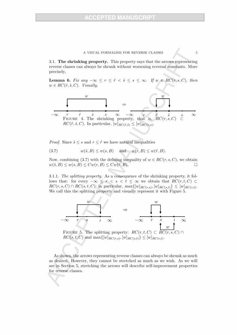
3.1. The shrinking property. This property says that the arrows representingreverse classes can always be shrunk without worsening reversal constants. Moreprecisely,

Lemma 6. Fix any −∞ ≤ r ≤ r < s ≤ s ≤ ∞. If w ∈ RC(r, s, C), thenw ∈ RC(r, s, C). Visually,

r sr

⇒w w

s −∞ ∞−∞ ∞ r sr sFigure 4. The shrinking property, that is, RC(r, s, C) ⊂RC(r, s, C). In particular, [w]RC(r,s) ≤ [w]RC(r,s).

Proof. Since s ≤ s and r ≤ r we have natural inequalities

(3.7) w(s, B) ≤ w(s,B) and w(r,B) ≤ w(r, B).

Now, combining (3.7) with the defining inequality of w ∈ RC(r, s, C), we obtainw(s, B) ≤ w(s,B) ≤ Cw(r,B) ≤ Cw(r, B).

3.1.1. The splitting property. As a consequence of the shrinking property, it fol-lows that: for every −∞ ≤ r < s < t ≤ ∞ we obtain that RC(r, t, C) ⊂RC(r, s, C) ∩ RC(s, t, C); in particular, max[w]RC(r,s), [w]RC(s,t) ≤ [w]RC(r,t).We call this the splitting property and visually represent it with Figure 5.

⇒

r s r st t

ww

w

−∞ ∞ −∞ ∞

Figure 5. The splitting property: RC(r, t, C) ⊂ RC(r, s, C) ∩RC(s, t, C) and max[w]RC(r,s), [w]RC(s,t) ≤ [w]RC(r,t).

As shown, the arrows representing reverse classes can always be shrunk as muchas desired. However, they cannot be stretched as much as we wish. As we willsee in Section 5, stretching the arrows will describe self-improvement propertiesfor reverse classes.


3.2. The concatenation property. This property provides the converse tothe splitting property. It says that whenever an arrow begins where anotherends, then they can be concatenated. Moreover, the reversal constant for theconcatenation is controlled by the product of the reversal constants involved.

Lemma 7. Fix any −∞ ≤ r < s < t ≤ ∞. If w ∈ RC(r, s, C1) ∩ RC(s, t, C2),then w ∈ RC(r, t, C1C2). Consequently, RC(r, s) ∩RC(s, t) = RC(r, t).

Bearing in mind that there is no distinction between arrows drawn above orbelow the extended real line, the statement of Lemma 7 can be visually recast asfollows:

−∞ ∞r ts−∞ ∞r ts

⇔

w

w

w

Figure 6. The concatenation property. Quantitatively,[w]RC(r,t) ≤ [w]RC(r,s)[w]RC(s,t).

Notice that the concatenation property together with the splitting propertyimply that RC(r, s) ∩RC(s, t) = RC(r, t).

Proof of Lemma 7. Since w ∈ RC(r, s, C1) ∩ RC(s, t, C2), we have w(t, B) ≤C2w(s,B) ≤ C1C2w(r,B).

3.3. The scaling property. This property dictates how reverse classes andreversal constants behave under the operation of taking powers. More precisely,

Theorem 8. Let −∞ ≤ r < s ≤ ∞ and fix w ∈ RC(r, s, C). Then,

(i) for any θ > 0, we have wθ ∈ RC( rθ ,sθ , C

θ),(ii) for any θ < 0, we have wθ ∈ RC( sθ ,

rθ , C

|θ|).

Visually, this is illustrated in Figure 7.


rθ

r s

⇔

w wθ

sθ

−∞ ∞−∞ ∞

sθ

r s

⇔

w

rθ

−∞ ∞−∞ ∞

θ > 0

θ < 0wθ

Figure 7. The scaling property. Quantitatively, [wθ]RC(r/θ,s/θ) =

[w]θRC(r,s), for θ > 0; and [wθ]RC(s/θ,r/θ) = [w]|θ|RC(r,s), for θ < 0.

Proof. Let us prove (i). Since w ∈ RC(r, s, C), given B ∈ BΩ we have

(3.8) w(s,B) =(

1µ(B)

∫

Bwθ

sθ dµ

)1/s

≤ Cw(r,B) = C

(1

µ(B)

∫

Bwθ

rθ dµ

)1/r

.

For θ > 0 we get(

1µ(B)

∫

Bwθ

sθ dµ

)θ/s≤ Cθ

(1

µ(B)

∫

Bwθ

rθ dµ

)θ/r,

that is, wθ ∈ RC( rθ ,sθ , C

θ). To prove (ii), we use (3.8) again, but now with θ < 0(

1µ(B)

∫

Bwθ

sθ dµ

)θ/s≥ Cθ

(1

µ(B)

∫

Bwθ

rθ dµ

)θ/r,

that is, wθ ∈ RC( sθ ,rθ , C

|θ|). Remark 9. It is convenient to point out that, during the formal manipulations,the axioms above provide qualitative as well as quantitative information aboutthe reverse classes and their weights. Meaning that when a particular weight issubjected to a sequence of axioms of the visual formalism, there will always bean explicit control on the reversal constants.

4. Some well-known reverse classes

Definition 10. Let 1 < s ≤ ∞. A weight w is said to belong to RHs, the reverseHolder class of order s, if the following inequality holds

[w]RHs := supB∈BΩ

w(s,B)w(1, B)−1 <∞.

In other words, RHs = RC(1, s). Visually,


s

w ∈ RHs⇔

s > 1

w

−∞ 0 1−1 ∞Figure 8. The RHs classes. Notice that RHs = RC(1, s).

Definition 11. Let 1 < p <∞. A weight w is said to belong to the Muckenhouptclass Ap if

[w]Ap := supB∈BΩ

w(1, B)w(

11− p,B

)−1

<∞.

In other words, Ap = RC(1/(1− p), 1). We write w ∈ A1 if

[w]A1 := supB∈BΩ

w(1, B)w(−∞, B)−1 <∞.

That is, A1 = RC(−∞, 1). Finally, we write w ∈ A∞ if

(4.9) [w]A∞ := supB∈BΩ

w(1, B)w(0, B)−1 <∞.

That is, A∞ = RC(0, 1). Again, we have chosen to use the notation Ap insteadof Ap(Ω). Muckenhoupt classes can be visually represented by the followingdiagrams in Figure 9.


11−p

11−p

w ∈ A1

w ∈ Ap

w ∈ A2

w ∈ Ap

w ∈ A∞

⇔

⇔

⇔

⇔

⇔

1 < p < 2

2 < p <∞

w

w

w

w

w

−∞ 0 1−1 ∞

−∞ 0 1−1 ∞

−∞ 0 1−1 ∞

−∞ 0 1−1 ∞

−∞ 0 1−1 ∞Figure 9. The Ap classes as reverse classes: Ap = RC((1− p)−1, 1).

Again, we refer the reader to [14, Chapter 7], [16, Chapter IV], [18, Chapter9], [27, Chapter 2], [34], [38, Chapter 5], [39, Chapters I and II], [40, ChapterIX], as well as references therein, for all the basic material and history of reverseHolder classes and Muckenhoupt weights.

Remark 12. The constant [w]A∞ in (4.9) was introduced by Hruscev in [21].Another constant, which has lately received a lot of attention, given by

(4.10) [w]′A∞ := supB∈BΩ

1µ(B)

∫

BM(wχB) dµ,

whereM stands for the Hardy-Littlewood maximal operator, was introduced byFujii [15] and Wilson [41]. The constant [w]′A∞ also characterizes A∞. Moreprecisely, in the Euclidean setting (with Ω = Rn), Hytonen and Perez proved in


[22] that one has [w]′A∞ ≤ cn[w]A∞ , for some dimensional constant cn > 0. Acorresponding inequality was proved in the context of spaces of homogeneous typeby Hytonen, Perez, and Rela in [23]. The study of A∞ through the constant [w]′A∞seems to be better suited for obtaining sharp reversal constants and reversalexponents, see [22, 23], and references therein.

4.1. Some practice. With the purpose of getting some practice with the visualformalism, next we go over some well-known properties of Ap weights (see, forinstance, [25, Section 1] and [11]).

It will be useful to bear in mind Remark 9 as well as the facts that, for 1 <p <∞, Ap = RC((1− p)−1, 1), A1 = RC(−∞, 1), and A∞ = RC(0, 1).

Corollary 13. Fix 1 < p < ∞ and let p′ denote its Holder conjugate, that is,1p + 1

p′ = 1. Then w ∈ Ap if and only if w1−p′ ∈ Ap′. Moreover, [w1−p′ ]Ap′ =

[w]p′−1Ap

.

Proof. This proof uses only the scaling property along with the fact that (1 −p)(1− p′) = 1.

w ∈ Ap w1−p′ ∈ Ap′

⇔Scalingw w1−p′

1 111−p′

11−p

m m

Figure 10. Visual proof of Corollary 13

Notice that, since scaling by a power θ has the effect of raising reversal con-stants to the power |θ| (see Theorem 8), for the sequence of steps, from left toright, in Figure 10 we have scaled by θ = 1− p′ < 0, yielding

[w1−p′ ]Ap′ ≤ [w]p′−1Ap′

.

Conversely, taking the steps in Figure 10 from right to left we have scaled byθ = 1− p < 0, giving

[w]Ap ≤ [w1−p′ ]p−1Ap′

.

Hence, [w1−p′ ]Ap′ = [w]p′−1Ap

.

Corollary 14. Fix 1 < p < ∞. Then, w ∈ A1 implies w1−p ∈ Ap ∩ RH∞, andwe have max[w1−p]Ap , [w1−p]RH∞ ≤ [w]p−1

A1. Conversely, w1−p ∈ Ap ∩ RH∞

implies w ∈ A1, and we have [w]A1 ≤ ([w1−p]Ap [w1−p]RH∞)1p−1 .


Proof. Here is the visual proof

w ∈ A1 w1−p ∈ Ap ∩RH∞

m

1

w

Scaling

w1−p⇔ ⇔

11−p

−∞ ∞ 111−p

Splitting

w1−p

Concatenating/

∞

m

w1−p


Again, by Theorem 8 and since shrinkage does not worsen reversal constants,for the left-to-right sequence of steps in Figure 11, we have: scaling (with θ =1−p < 0), which yields [w1−p]RC(1/(1−p),∞) = [w]p−1

A1, followed by splitting, which

then yields

max[w1−p]Ap , [w1−p]RH∞ ≤ [w]p−1

A1.

On the other hand, now considering the right-to-left sequence of steps, we have:concatenation, which yields [w1−p]RC(1/(1−p),∞) ≤ [w1−p]Ap [w1−p]RH∞ , followed

by scaling (with θ = 1/(1−p) < 0), which yields [w]A1 ≤ ([w1−p]Ap [w1−p]RH∞)1p−1 .

Corollary 15. Fix 1 < s < ∞. If w ∈ A1 ∩ RHs, then w1−p ∈ Aq ∩ RH∞ forevery 1 < p <∞ and q > (p− 1)/s+ 1. Moreover, max[w1−p]Aq , [w1−p]RH∞ ≤([w]A1 [w]RHs)p−1.

Proof. Let us start with the visual proof, which is immediate after realizing thatthe relation between the indices can be recast as s

1−p <1

1−q . We have


w ∈ A1 ∩RHs

w⇔ ⇔

Concatenating/

−∞ 1 s

w

s−∞

w

m Scaling

w1−p

∞s1−p

⇐Shrinking

s1−p

11−q

∞

w1−p

⇔

11 ∞

w1−p

w1−p

11−q

Splitting

Concatenating/Splitting

w1−p ∈ Aq ∩RH∞

m


For the clockwise sequence of steps in Figure 12 we have: first concatenation,which yields [w]RC(−∞,s) ≤ [w]A1 [w]RHs , followed by scaling (with θ = 1 − p),yielding [w1−p]RC(s/(1−p),∞) ≤ ([w]A1 [w]RHs)p−1, followed by shrinking, whichgives [w1−p]RC(1/(1−q),∞) ≤ ([w]A1 [w]RHs)p−1, and finally, splitting gives

max[w1−p]Aq , [w1−p]RH∞ ≤ ([w]A1 [w]RHs)

p−1.

Corollary 16. Fix 1 < p <∞. Then, w ∈ Ap ∩ RH∞ implies that w1−p′ ∈ A1,with [w1−p′ ]A1 ≤ ([w]RH∞ [w]Ap)p

′−1. Conversely, w1−p′ ∈ A1 implies w ∈ Ap ∩RH∞, with max[w]RH∞ , [w]Ap ≤ [w1−p′ ]p−1

A1.

Proof. Figure 13 illustrates the visual proof


w ∈ Ap ∩RH∞

m

1

w

11−p

∞

⇔Concatenating/

w

11−p

∞ −∞ 1

w

w1−p′⇔Scaling m

w1−p′ ∈ A1

Splitting


The proof here closely follows the proof of Corollary 14 along with the fact that(1− p)(1− p′) = 1. For the left-to-right sequence of steps in Figure 13 we have:concatenation, which yields [w]RH(1/(1−p),∞) ≤ [w]Ap [w]RH∞ and then scaling by1− p′ < 0, which gives [w1−p′ ]A1 ≤ ([w]Ap [w]RH∞)p

′−1.For the right-to-left sequence of steps in Figure 13 we have: scaling by 1

1−p′ =

1− p, which yields [w]RH(1/(1−p),∞) = [w1−p′ ]p−1A1

and then splitting, which gives

max[w]RH∞ , [w]Ap ≤ [w1−p′ ]p−1A1

.

Corollary 17. Let 1 < p, s <∞ and set q := s(p− 1) + 1. Then, w ∈ Ap ∩RHs

implies ws ∈ Aq, with [ws]Aq ≤ ([w]Ap [w]RHs)s. Conversely, ws ∈ Aq impliesw ∈ Ap ∩RHs, with max[w]Ap , [w]RHs ≤ [ws]1/sAq

.

Proof. Figure 14 illustrates the visual proof

w ∈ Ap ∩RHs

m

1

w

11−p

∞

⇔Concatenating/

w

11−p

∞ 1

w

ws⇔Scaling m

ws ∈ Aq

Splitting

s s 1s(1−p) = 1

1−q


In Figure 14, from left to right, we have: concatenation, which gives[w]RC(1/(1−p),s ≤ [w]Ap [w]RHs , followed by scaling by s, which gives


[ws]Aq ≤ ([w]Ap [w]RHs)s. From right to left we have: scaling by 1/s, yielding[w]RC(1/(1−p),s) = [ws]1/sAq

, followed by splitting, which gives max[w]Ap , [w]RHs ≤[ws]1/sAq

.

5. Self-improving properties

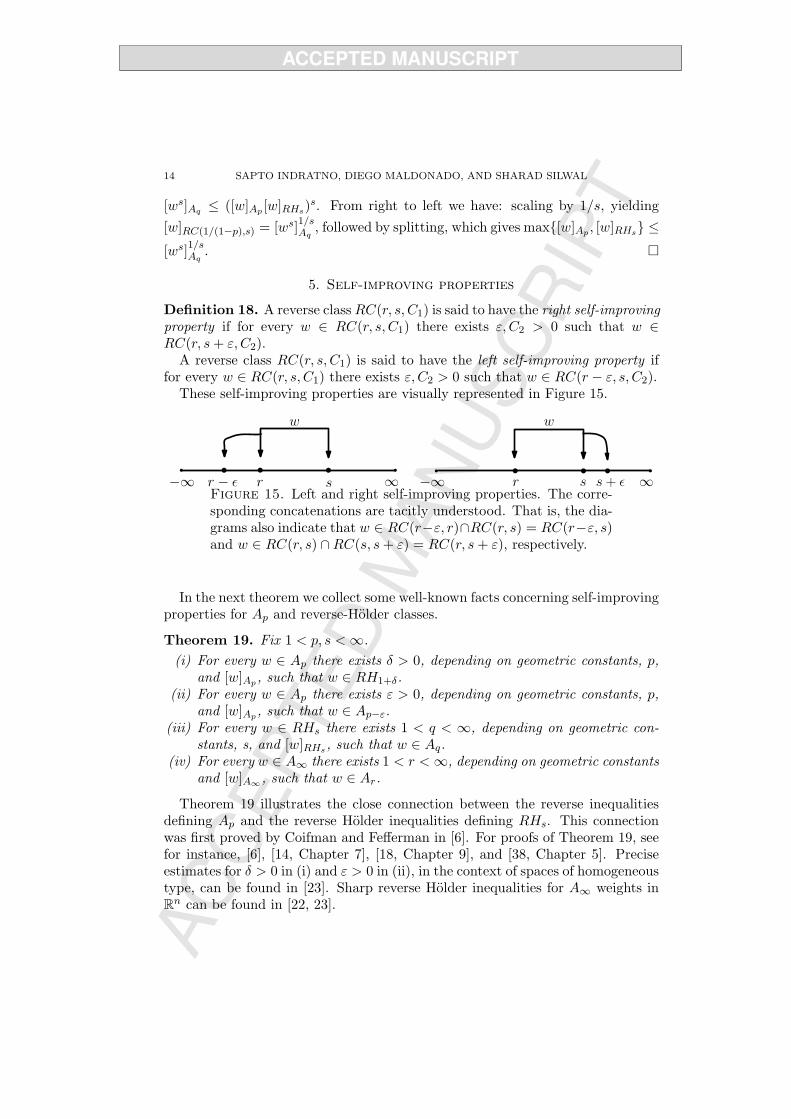
Definition 18. A reverse classRC(r, s, C1) is said to have the right self-improvingproperty if for every w ∈ RC(r, s, C1) there exists ε, C2 > 0 such that w ∈RC(r, s+ ε, C2).

A reverse class RC(r, s, C1) is said to have the left self-improving property iffor every w ∈ RC(r, s, C1) there exists ε, C2 > 0 such that w ∈ RC(r − ε, s, C2).

These self-improving properties are visually represented in Figure 15.

r s s + εr sr − ε

w w

−∞ ∞−∞ ∞Figure 15. Left and right self-improving properties. The corre-sponding concatenations are tacitly understood. That is, the dia-grams also indicate that w ∈ RC(r−ε, r)∩RC(r, s) = RC(r−ε, s)and w ∈ RC(r, s) ∩RC(s, s+ ε) = RC(r, s+ ε), respectively.

In the next theorem we collect some well-known facts concerning self-improvingproperties for Ap and reverse-Holder classes.

Theorem 19. Fix 1 < p, s <∞.(i) For every w ∈ Ap there exists δ > 0, depending on geometric constants, p,

and [w]Ap, such that w ∈ RH1+δ.(ii) For every w ∈ Ap there exists ε > 0, depending on geometric constants, p,

and [w]Ap, such that w ∈ Ap−ε.(iii) For every w ∈ RHs there exists 1 < q < ∞, depending on geometric con-

stants, s, and [w]RHs, such that w ∈ Aq.(iv) For every w ∈ A∞ there exists 1 < r <∞, depending on geometric constants

and [w]A∞, such that w ∈ Ar.Theorem 19 illustrates the close connection between the reverse inequalities

defining Ap and the reverse Holder inequalities defining RHs. This connectionwas first proved by Coifman and Fefferman in [6]. For proofs of Theorem 19, seefor instance, [6], [14, Chapter 7], [18, Chapter 9], and [38, Chapter 5]. Preciseestimates for δ > 0 in (i) and ε > 0 in (ii), in the context of spaces of homogeneoustype, can be found in [23]. Sharp reverse Holder inequalities for A∞ weights inRn can be found in [22, 23].


We can now illustrate the contents of Theorem 19 as follows

w

1 1 + δ11−p

w

111−p

11−(p−ε)

w

1 s11−q

w

1011−r

0 0

0

(i) (ii)

(iii) (iv)Figure 16. The self-improving properties for the Ap classes asstated in Theorem 19. Notice that the “improvement leaps” inparts (i), (ii), and (iv) will typically be small. That is, δ andε will be small and r will be big. However, in the case of (iii),although the index q will also be typically large, the “improvementleap” is of length larger than one, crossing from 1 all the way backto the negative number 1

1−q .

In order to keep practicing our visual formalism, let us prove some well-knownresults using the diagrams for self-improving properties.

Corollary 20. Fix 1 < s <∞. If w ∈ RHs then ws ∈ A∞.

Proof. The visual proof is illustrated in Figure 17. Notice how the first step usesthe self-improving property from Theorem 19 (iii).


w ws

s111−q

⇔Scaling

1s(1−q)

0 1

w ∈ RHs ⇔

⇓ Shrinking

ws

10

⇔ws ∈ A∞

0

Figure 17. Proof of Corollary 20.

Corollary 21. Fix 1 < s < ∞. If w ∈ RHs, then there exists t > s such thatw ∈ RC(0, t) ⊂ RHt.

Proof. The visual proof is illustrated in Figure 18. Again, the first step uses theself-improving property from Theorem 19 (iii).

w ws

s111−q

⇔Scaling

1s(1−q) 0 1

w ∈ RHs ⇔

⇓ Shrinking and

ws

10

⇔w ∈ RC(0, t)⇔

0

self-improving

1 + δ

Scalingw

s s(1 + δ)0 1

Figure 18. Proof of Corollary 21 with t := s(1 + δ).

Corollary 22. If w ∈ A∞, then there exists ε > 0 such that wε ∈ A2.

Proof. The visual proof is illustrated in Figure 19. Notice how the first step usesthe self-improving property from Theorem 19 (iv).


w w

1011−r

−1

⇒Shrinking

11−r

0 1r−1

w ∈ A∞ ⇔

1−1

m Scaling

w1

r−1

−1 10

⇔w1

r−1 ∈ A2

Figure 19. Proof of Corollary 22 with ε := 1r−1 .

Weak reverse classes also enjoy self-improving properties. For instance, wehave

Theorem 23. Fix 1 < s <∞ and 0 < p < q < r ≤ ∞. Then,(i) for every w ∈ RHweak

s there exists ε > 0 such that w ∈ RHweaks+ε , and

(ii) RCweak(q, r) = RCweak(p, r).Visually, these properties are depicted in Figures 20 and 21.

1 s s + ε0

w

−∞ ∞Figure 20. The self-improving property for the weak reverseclass RHweak

s from Theorem 23 (i).

0 p q rq r0

⇔w w

−∞ ∞ −∞ ∞Figure 21. The self-improving property for RCweak(q, r) fromTheorem 23 (ii).


The whole phenomenon of reverse inequalities and their self-improving prop-erties stems from Gehring’s work [17] (see [2, Chapter 3] for an exposition of theso-called Gehring’s lemma in doubling metric spaces). As mentioned, the con-nection between reverse Holder inequalities and Ap weights was first explored in[6]. A proof for Theorem 23 (i) in spaces of homogeneous type can be found, forinstance, in [28]. A proof for Theorem 23 (ii) in spaces of homogeneous type canbe found, for instance, in [3, Lemma 1.4] and the case r = ∞ has been workedout, for instance, in [29, Remark 4.4].

6. Reverse classes, BMO, BLO, and BUO

Throughout this section we will consider Ω = X.

Definition 24. We recall the definitions of BMO, BLO and BUO; namely, thespaces of functions of bounded mean oscillation, bounded lower oscillation, andbounded upper oscillation, respectively. w ∈ BMO if and only if

‖w‖BMO := supB∈BΩ

(1

µ(B)

∫

B|w − wB| dµ

)<∞,

where, as usual, wB :=(

1µ(B)

∫B w dµ

). w ∈ BLO if and only if

‖w‖BLO := supB∈BΩ

(1

µ(B)

∫

B(w − ess inf

Bw) dµ

)<∞.

w ∈ BUO if and only if

‖w‖BUO := supB∈BΩ

(1

µ(B)

∫

B(ess sup

Bw − w) dµ

)<∞.

Proposition 25 below provides characterizations of BMO and BLO in termsof Ap classes.

Proposition 25. The following characterizations hold true:(i) logw ∈ BMO if and only if wα ∈ Ap for some 1 < p <∞ and some α ∈ R.

(ii) logw ∈ BLO if and only if wε ∈ A1 for some ε > 0.(iii) logw ∈ BUO if and only if wε ∈ RH∞ for some ε > 0.

For a proof of (i) see, for instance, [14, p.151], [18, p.300], and [38, p.218].The proof of (ii) can be found in [8, Lemma 1]. The proof of (iii) follows, forinstance, from the characterization RH∞ = eBUO as in [36, Theorem 3.2]. Inview of Proposition 25, we have

Corollary 26. The following characterizations hold true:(i) logw ∈ BMO if and only if w ∈ RC(r, s) for some −∞ ≤ r < s ≤ ∞.

(ii) logw ∈ BLO if and only if w ∈ RC(−∞, r) for some −∞ < r ≤ ∞.(iii) logw ∈ BUO if and only if w ∈ RC(r,∞) for some −∞ ≤ r <∞.


Visually,

log w ∈ BMO ⇔

r

w

s−∞ ∞

Figure 22. A characterization of BMO: BMO = log

(⋃

−∞≤r<s≤∞RC(r, s)

).

log w ∈ BLO ⇔

−∞ ∞r

w

Figure 23. A characterization of BLO: BLO = log

(⋃

−∞<r≤∞RC(−∞, r)

).

log w ∈ BUO ⇔

r

w

−∞ ∞

Figure 24. A characterization of BUO: BUO = log

(⋃

−∞≤r<∞RC(r,∞)

).

Proof. Here is the visual proof of Corollary 26 by means of Proposition 25.

1

⇔log w ∈ BMO ⇔

011−q

wr ∈ Aq ⇔1r01

r(1−q)

wr w

Figure 25. Proof of the “only if” part of Corollary 26 (i), for0 < r, using Proposition 25 (i). In the case of r < 0, only thepositions of the points 1/r and 1/(r(1−q)) will be switched in thefigure.


w wr

r s 1 sr

11−q

⇔ wr ∈ Aq

0 0

⇔ log w ∈ BMO⇔

Figure 26. Proof of the “if” part of Corollary 26 (i), for 0 < r <s, by using Proposition 25 (i). The case r < s < 0 reduces to thiscase after scaling by −1. By the shrinking property, the generalcase r < s reduces to one of the previous two cases (see Exercise5 in Section 10).

w wr

0 r 1−∞−∞ 0

⇔Scaling

⇔ log w ∈ BLO

Figure 27. Proof of Corollary 26 (ii) for the case r > 0, by usingProposition 25 (ii).

−∞ r 0 0 1 ∞11−q

w wr w

−∞ 0 1r(1−q)

⇔ ⇔

Scaling and

Scalingself-improving

Figure 28. Proof of Corollary 26 (ii) for the case r < 0. It isshown how after scaling and self-improving, this case reduces tothe case r > 0.

The proof of Corollary 26 (iii) is left as an exercise (see Exercise 6 in Section10).

7. Interpolation

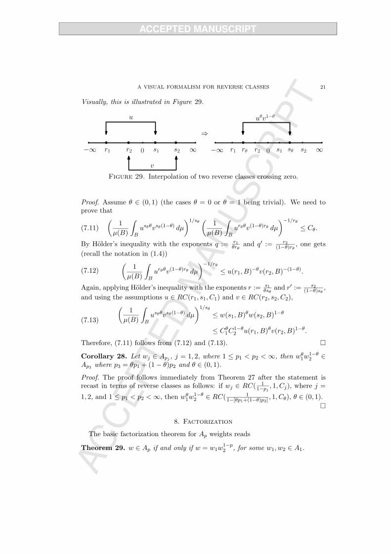
Theorem 27. Let r1 ≤ r2 < 0 < s1 ≤ s2, and u ∈ RC(r1, s1, C1) and v ∈RC(r2, s2, C2). Then, for every θ ∈ [0, 1], we have uθv1−θ ∈ RC(rθ, sθ, Cθ),where Cθ := Cθ1C

1−θ2 and

1rθ

:=θ

r1+

1− θr2

< 0,1sθ

:=θ

s1+

1− θs2

> 0.


Visually, this is illustrated in Figure 29.

⇒

u

∞−∞ r1 s2

uθv1−θ

0

v

s1r2 ∞−∞ r1 s20 s1r2rθ sθ

Figure 29. Interpolation of two reverse classes crossing zero.

Proof. Assume θ ∈ (0, 1) (the cases θ = 0 or θ = 1 being trivial). We need toprove that

(7.11)(

1µ(B)

∫

Busθθvsθ(1−θ) dµ

)1/sθ(

1µ(B)

∫

Burθθv(1−θ)rθ dµ

)−1/rθ

≤ Cθ.

By Holder’s inequality with the exponents q := r1θrθ

and q′ := r2(1−θ)rθ , one gets

(recall the notation in (1.4))(

1µ(B)

∫

Burθθv(1−θ)rθ dµ

)−1/rθ

≤ u(r1, B)−θv(r2, B)−(1−θ).(7.12)

Again, applying Holder’s inequality with the exponents r := s1θsθ

and r′ := s2(1−θ)sθ ,

and using the assumptions u ∈ RC(r1, s1, C1) and v ∈ RC(r2, s2, C2),(

1µ(B)

∫

Busθθvsθ(1−θ) dµ

)1/sθ

≤ w(s1, B)θw(s2, B)1−θ

≤ Cθ1C1−θ2 u(r1, B)θv(r2, B)1−θ.

(7.13)

Therefore, (7.11) follows from (7.12) and (7.13).

Corollary 28. Let wj ∈ Apj , j = 1, 2, where 1 ≤ p1 < p2 < ∞, then wθ1w1−θ2 ∈

Ap3 where p3 = θp1 + (1− θ)p2 and θ ∈ (0, 1).

Proof. The proof follows immediately from Theorem 27 after the statement isrecast in terms of reverse classes as follows: if wj ∈ RC( 1

1−pj , 1, Cj), where j =

1, 2, and 1 ≤ p1 < p2 <∞, then wθ1w1−θ2 ∈ RC( 1

1−[θp1+(1−θ)p2] , 1, Cθ), θ ∈ (0, 1).

8. Factorization

The basic factorization theorem for Ap weights reads

Theorem 29. w ∈ Ap if and only if w = w1w1−p2 , for some w1, w2 ∈ A1.


Theorem 29 was first proved, in the Euclidean setting, by P. Jones in [26] andother proofs then appeared in [7, 37]. For a proof in spaces of homogeneoustype, see [39, Chapter II]. A thorough discussion of this topic can be found, forinstance, in [12, Sections 1.1 and 6.2], [14, Section 5.5], and [40, Chap IX].

The visual rendition of the factorization theorem yields a certain intersectionproperty for the arrows, see Figure 30.

111−p

∞1011−p

−∞1−∞

w1, w2

0

w1

w1−p2

w1w1−p2

⇔⇔Scaling Factorization

0

Figure 30. The factorization of Ap weights as an intersectionproperty for the arrows.

Theorem 29 can be extended as follows:

Theorem 30. Let r < 0 < s. Then w ∈ RC(r, s) if and only if w = uv for someu ∈ RC(r,∞) and v ∈ RC(−∞, s). Visually,

−∞ ∞r s−∞ ∞r s

⇔

v

u

w = uv

0 0

Figure 31. The factorization of a weight w belonging to a reverseclass crossing zero as an intersection property for the arrows.

Proof. For the ‘if’ part, we take u ∈ RC(r,∞, C2) and v ∈ RC(−∞, s, C1) andwe will prove uv ∈ RC(r, s, C1C2), that is,

(8.14) (uv)(s,B) ≤ C1C2 (uv)(r,B) ∀B ∈ BΩ.

Using the assumptions u ∈ RC(r,∞, C2) and v ∈ RC(−∞, s, C1), given B ∈ BΩ

we have

(8.15) (uv)(s,B) ≤ (ess supB

u)v(s,B) ≤ C2 u(r,B)v(s,B)

and

(8.16) (uv)(r,B)−1 ≤ (ess infB

v)−1u(r,B)−1 ≤ C1 v(s,B)−1u(r,B)−1.


Hence, the estimate (8.14) follows by multiplying (8.15) and (8.16).For the ‘only if’ part, we take w ∈ RC(r, s) and need to show that there

exist u ∈ RC(r,∞) and v ∈ RC(−∞, s) such that w = uv. We know thatw ∈ RC(r, s), then, by Theorem 8 (scaling), we have ws ∈ Ap, with p := (1 −sr ) > 1. Then, by Theorem 29 (factorization), there exist u, v ∈ A1 such thatws = uv1−p. Defining u := u

1s and v := v

1−ps , we get ws = uv. Now, since

u, v ∈ A1 = RC(−∞, 1) and s > 0, by Theorem 8 (scaling), we have thatu := u

1s ∈ RC(−∞, s). On the other hand, since r = s

1−p , from the definition of

p, by scaling we have that v := v1−ps ∈ RC( s

1−p ,∞) = RC(r,∞).

Corollary 31. (See [8, Section III]) Every BMO function is the difference oftwo BLO functions, that is,

BMO = BLO −BLO.Proof. In light of Corollary 26 (i) and (ii), we only need to show that w ∈RC(r, s), for some r < 0 < s, if and only if w = w1w

−12 for some w1 ∈ RC(−∞, r1)

and w2 ∈ RC(−∞, r2), with r1, r2 > 0. Let r < 0 < s and w ∈ RC(r, s).Then, take w1 ∈ RC(−∞, s) and w2 ∈ RC(−∞,−r) provided by Theorem 30to get w = w1w

−12 . Conversely, let w1 ∈ RC(−∞, r1) and w2 ∈ RC(−∞, r2),

for some r1, r2 > 0. Finally, since −r2 < 0 < r1, by Theorem 30 we havew1w

−12 ∈ RC(−r2, r1).

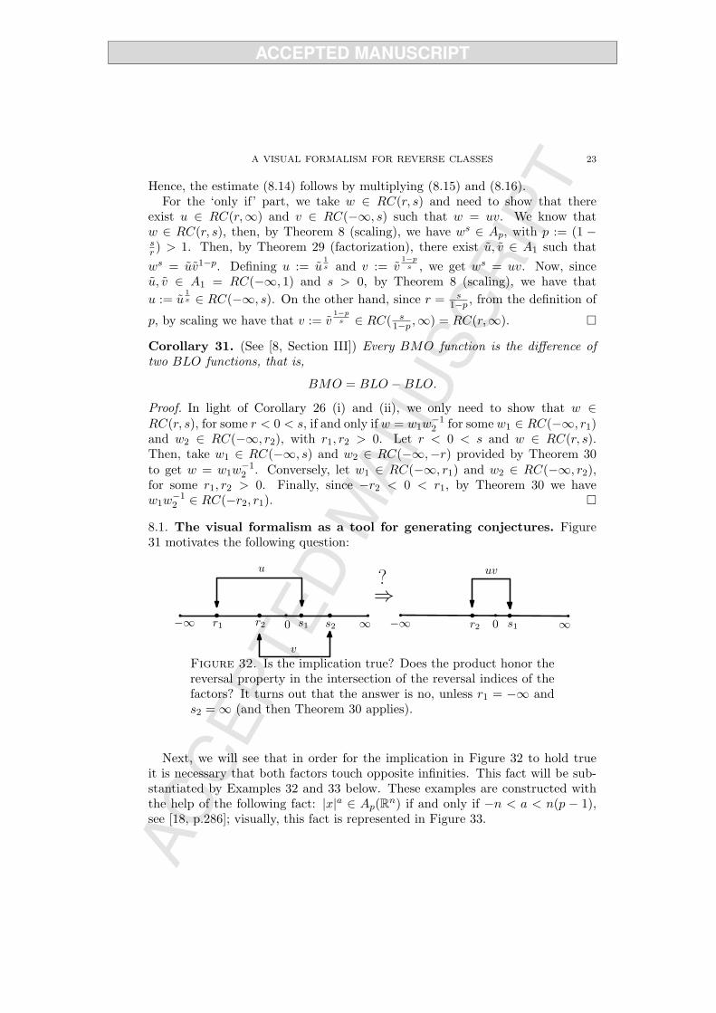
8.1. The visual formalism as a tool for generating conjectures. Figure31 motivates the following question:

u

v

uv

r1 r2 s1 s20 0r2 s1

⇒?

−∞ −∞ ∞∞

Figure 32. Is the implication true? Does the product honor thereversal property in the intersection of the reversal indices of thefactors? It turns out that the answer is no, unless r1 = −∞ ands2 =∞ (and then Theorem 30 applies).

Next, we will see that in order for the implication in Figure 32 to hold trueit is necessary that both factors touch opposite infinities. This fact will be sub-stantiated by Examples 32 and 33 below. These examples are constructed withthe help of the following fact: |x|a ∈ Ap(Rn) if and only if −n < a < n(p − 1),see [18, p.286]; visually, this fact is represented in Figure 33.


−n < a < n(p− 1)

1011−p

|x|a

⇔−∞ ∞

Figure 33. A necessary and sufficient condition for the powerweight |x|a to be in Ap(Rn).

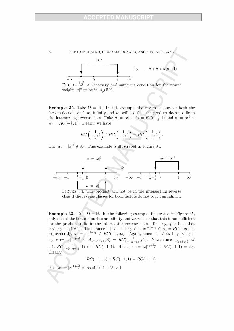
Example 32. Take Ω = R. In this example the reverse classes of both thefactors do not touch an infinity and we will see that the product does not lie inthe intersecting reverse class. Take u := |x| ∈ A3 = RC(−1

2 , 1) and v := |x|3 ∈A5 = RC(−1

4 , 1). Clearly, we have

RC

(−1

2, 1)∩RC

(−1

4, 1)

= RC

(−1

4, 1).

But, uv = |x|4 /∈ A5. This example is illustrated in Figure 34.

−∞ ∞−1 1

;

v := |x|3

u := |x|

0−12−1

4 −∞ ∞−1 10−12−1

4

uv = |x|4

Figure 34. The product will not be in the intersecting reverseclass if the reverse classes for both factors do not touch an infinity.

Example 33. Take Ω = R. In the following example, illustrated in Figure 35,only one of the factors touches an infinity and we will see that this is not sufficientfor the product to lie in the intersecting reverse class. Take ε0, ε1 > 0 so that0 < (ε0 + ε1) 1. Then, since −1 < −1 + ε0 < 0, |x|−1+ε0 ∈ A1 = RC(−∞, 1).Equivalently, u := |x|1−ε0 ∈ RC(−1,∞). Again, since −1 < ε0 + ε1

2 < ε0 +ε1, v := |x|ε0+

ε12 ∈ A1+ε0+ε1(R) = RC( 1

−(ε0+ε1) , 1). Now, since 1−(ε0+ε1)

−1, RC( 1−(ε0+ε1) , 1) ⊂⊂ RC(−1, 1). Hence, v := |x|ε0+

ε12 ∈ RC(−1, 1) = A2.

Clearly,

RC(−1,∞) ∩RC(−1, 1) = RC(−1, 1).

But, uv = |x|1+ε12 /∈ A2 since 1 + ε1

2 > 1.


−∞ ∞−1 1

;

v := |x|ε0+ε12

u := |x|1−ε0

01−(ε0+ε1)

uv = |x|1+ε12

−∞ ∞−1 101−(ε0+ε1)

Figure 35. The product will not be in the intersecting reverseclass if the reverse class of one of the factors fails to touch aninfinity.

9. Using the visual formalism to illustrate proofs of Harnack’sinequality

Fix an open set Ω ⊂ X. A weight w is said to satisfy Harnack’s inequality,with constant CH ≥ 1, in Ω if w ∈ RC(−∞,∞, CH), that is,

ess supB

w ≤ CH ess infB

w, ∀B ∈ BΩ.

That is, w satisfies the most extreme reversal inequality. Visually,

−∞ ∞

w

Figure 36. The Harnack class RC(−∞,∞).

In this section we use the visual formalism to provide a brief description ofMoser’s and Krylov-Safonov’s proofs of Harnack’s inequality for positive solu-tions to elliptic PDEs. While Moser’s method is most notable for his ingeniousiteration scheme [33] in the context of divergence-form operators, the Krylov-Safonov’s method, based on innovative probabilistic tools [30, 31], was developedin the context of non-divergence-form operators. Both of these models standas cornerstones in the study of regularity properties of solutions to PDEs andare flexible enough to be carried out in more general types of doubling quasi-metric spaces possessing suitable additional structure (e.g., carrying Sobolev orPoincare-type inequalities). In what follows the underlying space of homogeneoustype is Euclidean space Rn with Lebesgue measure (the latter indicated by | · |).

9.1. Moser’s iterations and Harnack’s inequality. Let Ω ⊂ Rn be an openbounded set and for each x ∈ Ω let A(x) be an n×n symmetric matrix verifying


the uniform ellipticity condition

(9.17) Λ1|ξ|2 ≤ 〈A(x)ξ, ξ〉 ≤ Λ2|ξ|2, ∀x ∈ Ω, ξ ∈ Rn,

for some constants 0 < Λ1 ≤ Λ2. Harnack’s inequality for positive solutions tothe divergence-form elliptic equation

Lu :=n∑

i,j=1

(aij(x)ui)j = div(A(x)∇u) = 0 in Ω ⊂ Rn

was established by J. Moser in [33]. Moreover, Moser showed that the Harnackconstant CH depends only on dimension n and the ratio Λ2/Λ1.

The first step in his approach is based on an interaction between a Sobolevinequality and an energy estimate (Caccioppoli’s inequality) to show that anypositive subsolution u (i.e., Lu ≥ 0 in Ω) satisfies u ∈ RCweak(2, 2ρ), whereρ := 2n/(n− 2) > 1. More precisely,

(9.18)(

1|B|

∫

Bu2ρ dx

) 12ρ

≤ C(n,Λ2/Λ1)(

1|B|

∫

2Bu2 dx

) 12

, ∀B ∈ BΩ.

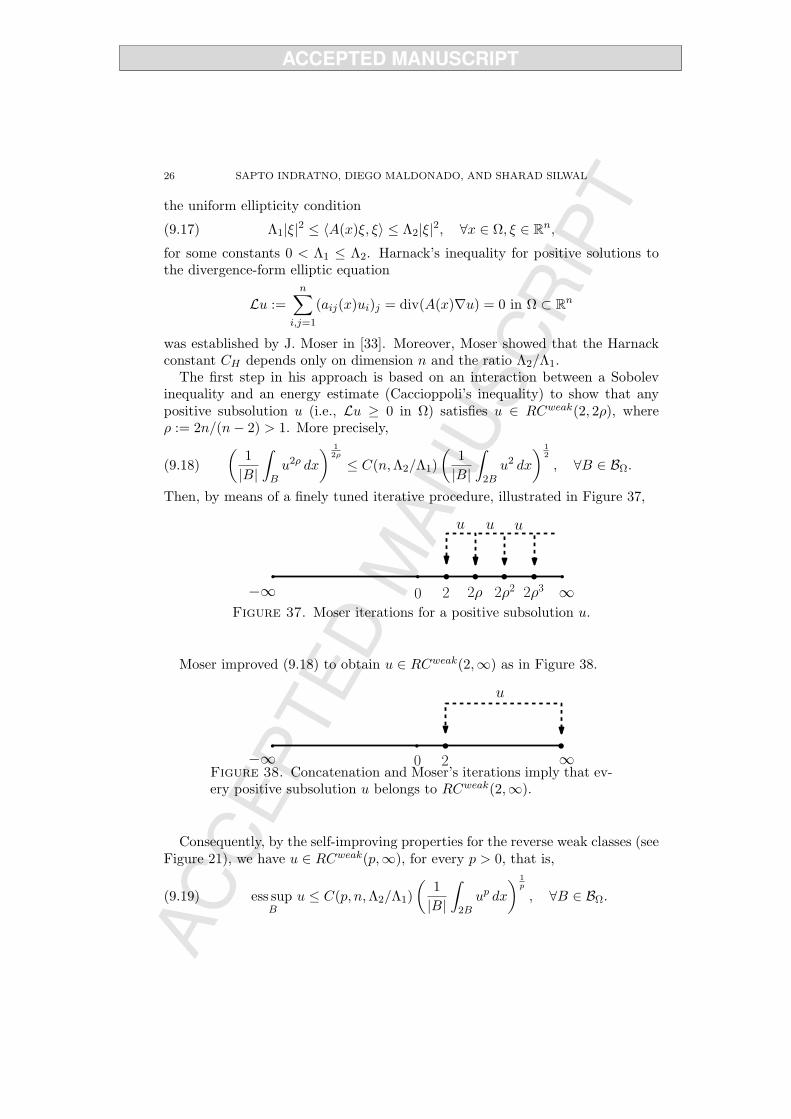
Then, by means of a finely tuned iterative procedure, illustrated in Figure 37,

u

−∞ 0 2 ∞2ρ 2ρ2 2ρ3

u u

Figure 37. Moser iterations for a positive subsolution u.

Moser improved (9.18) to obtain u ∈ RCweak(2,∞) as in Figure 38.

u

−∞ 0 2 ∞Figure 38. Concatenation and Moser’s iterations imply that ev-ery positive subsolution u belongs to RCweak(2,∞).

Consequently, by the self-improving properties for the reverse weak classes (seeFigure 21), we have u ∈ RCweak(p,∞), for every p > 0, that is,

(9.19) ess supB

u ≤ C(p, n,Λ2/Λ1)(

1|B|

∫

2Bup dx

) 1p

, ∀B ∈ BΩ.


as illustrated in Figure 39.

u

−∞ 0p ∞Figure 39. Every positive subsolution u belongs toRCweak(p,∞) for all p > 0.

Inequality (9.19) is usually referred to as the local boundedness property for uand it can also be proved by means of De Giorgi’s truncations. For both methods,Moser’s iterations and De Giorgi’s truncations, see for instance [20, Section 4.2].

Now, if u is a positive solution, then both u and u−1 are positive subsolutionsand (9.19) applied to them yields u ∈ RCweak(p,∞) and u−1 ∈ RCweak(p,∞).But, by the scaling property with θ = −1, the latter means u ∈ RCweak(−∞,−p),that is, for all p > 0,

(9.20)(

1|B|

∫

2Bu−p dx

)− 1p

≤ C(p, n,Λ2/Λ1) ess infB

u ∀B ∈ BΩ.

Hence, positive solutions satisfy both (9.19) and (9.20), this is illustrated inFigure 40.

u

−∞ 0−p

u

p ∞Figure 40. Every positive solution u belongs toRCweak(−∞,−p) ∩RCweak(p,∞) for all p > 0.

The next step in Moser’s Harnack inequality consists in establishing the exis-tence of p0 > 0 such that if u is a positive supersolution (i.e., Lu ≤ 0 in Ω), thenup0 ∈ A2(Ω). This is illustrated in Figure 41.


−p0 p0

u

−∞ 0 ∞Figure 41. There exists a structural p0 > 0 such that everypositive supersolution u (i.e., Lu ≤ 0) satisfies up0 ∈ A2. By thescaling property, this is equivalent to u ∈ RC(−p0, p0).

The step in Figure 41 is typically accomplished by using a Poincare inequalityand an energy estimate for log u to obtain that log u ∈ BMO(Ω). Then, byCorollary 22 and the techniques in the proof of Corollary 26 (i) (see also Exercise5 in Section 10), it follows that there is a p0 > 0 such that up0 ∈ A2.

Finally, by choosing the p in Figure 40 equal to the p0 in Figure 41 and using thefact that up0 is doubling, since it is A2, so that dashed lines in Figure 40 turn intosolid ones (see Remark 5), the concatenation property yields u ∈ RC(−∞,−p0)∩RC(−p0, p0) ∩RC(p0,∞) = RC(−∞,∞).

9.2. Krylov-Safanov’s approach to Harnack’s inequality. As before, letA(x) be a uniformly elliptic matrix satisfying (9.17). During the 1980’s, N.Krylov and M. Safonov took recourse to completely new measure-theoretic tools[30, 31] in order to establish Harnack’s inequality for positive solutions to thenon-divergence-form elliptic equation

(9.21) Lu :=n∑

i,j=1

aij(x)uij = tr(A(x)D2u) = 0 in Ω ⊂ Rn.

Later on, L. Caffarelli’s seminal work [4] on fully non-linear elliptic equations(see also [5, Section 4.2]) greatly enriched and simplified Krylov-Safonov theoryrendering it quite flexible and still manageable. This, in fact, paved the way forthe axiomatizations of the Krylov-Safonov theory in doubling quasi-metric spacescarried out in [1, 13, 24]. All these axiomatic approaches involve, implicitly orexplicitly, the so-called critical density and power-like decay properties.

Definition 34. Let KΩ denote a family of non-negative measurable functionswith domain contained in Ω. If u ∈ KΩ and A ⊂ dom(u) then we write u ∈KΩ(A), where dom(u) stands for the domain of the function u. Assume that KΩ

is closed under multiplication by positive scalars.Let 0 < ε < 1 ≤ M . KΩ is said to satisfy the critical density property with

constants ε and M if for every B2R(x0) ∈ BΩ and u ∈ KΩ(B2R(x0)) with

ess infBR(x0)

u ≤ 1,


it follows that

µ(x ∈ B2R(x0) : u(x) > M) ≤ εµ(B2R(x0)).

Let 0 < % < 1 < N . KΩ is said to satisfy the power-like decay property withconstants N and % if for every B2R(x0) ∈ BΩ and every u ∈ KΩ(B2R(x0)) with

ess infBR(x0)

u ≤ 1,

it follows that

µ(x ∈ BR/2(x0) : u(x) > Nk) ≤ %kµ(BR/2(x0)) ∀k ∈ N.

In the context of the non-divergence form elliptic operators (9.21), the crit-ical density property plays the role analogous to the Moser iterations in thedivergence-form setting. Indeed, let KΩ denote the class of supersolutions of(9.21) (that is, u ∈ KΩ if and only if Lu ≤ 0 in Ω), as a first step it is provedthat KΩ possesses the critical density property; see, for instance, Theorem 2.1.1on page 31 of [19]. Then, it is proved that if for any given ball B ∈ BΩ and anyscalar λ with λ − u > 0 in B we have λ − u ∈ KΩ, then u ∈ RCweak(p,∞) forevery p > 0. See, for instance [24, Section 3]. Therefore, putting these two resultstogether, if u is a positive subsolution (Lu ≥ 0), then L(λ − u) = −Lu ≤ 0, sothat λ − u ∈ KΩ and, consequently, u ∈ RCweak(p,∞) for every p > 0. This isillustrated in Figure 42.

u

−∞ 0p ∞Figure 42. The critical density property implies that every pos-itive subsolution u (i.e. Lu ≥ 0) belongs to RCweak(p,∞) for allp > 0.

The next key step in the Krylov-Safonov’s approach consists in showing thatthe class of positive supersolutions possesses the power-like decay property, seefor instance Theorem 2.1.3 on page 36 of [19] and Lemma 4.6 on page 33 of [5].Now, the fact that the class of supersolutions has the power-like decay property(and since it is closed under multiplication by positive constants) amounts tothe existence of constants 0 < δ < 1 ≤ C, depending only on %, N , Λ2/Λ1,and dimension n, such that every supersolution u satisfies the reverse inequalityRC(−∞, δ, C) (see [24, Remark 2]); namely,

(9.22)1|B|

∫

Buδ dx ≤ Cδ ess inf

Buδ ∀B ∈ BΩ.


In other words, uδ ∈ A1(Ω). Inequality (9.22) is usually referred to as the weakHarnack inequality for u and it is here illustrated in Figure 43.

u

−∞ 0 δ ∞Figure 43. There exists a structural δ > 0 such that every posi-tive supersolution u (i.e., Lu ≤ 0) satisfies uδ ∈ A1. By the scalingproperty, this is equivalent to u ∈ RC(−∞, δ).

Finally, if u is a positive solution in Ω, then it is both a subsolution and asupersolution and by choosing the p in Figure 42 equal to the δ in Figure 43(and using the fact that uδ is doubling, since it is A1, turns the dashed arrow inFigure 42 into a solid one), the concatenation property yields u ∈ RC(−∞, δ) ∩RC(δ,∞) = RC(−∞,∞).

10. Further practice

Exercise 1. Prove that the three axioms of the visual formalism for the reverseclasses RC(r, s) also apply to the weak reverse classes RCweak(r, s) and studythe behavior of the weak-reversal constants.

Exercise 2. Use the visual formalism to prove that if w ∈ A∞ and wr ∈ A1 forsome 0 < r <∞, then w ∈ A1. Estimate [w]A1 in terms of [w]A∞ and [wr]A1 byconsidering the cases r > 1 and 0 < r < 1.

Exercise 3. Fix 1 < s < ∞. Use the visual formalism to prove that ws ∈ A∞implies w ∈ RHs with [w]RHs ≤ [ws]1/sA∞ .

Exercise 4. Prove Theorem 30 using the visual formalism.

Exercise 5. Use the techniques depicted in Figures 26 and 28 to prove that everyweight satisfying a reverse inequality “must cross the exponent zero”. That is,if w ∈ RC(r, s) for some −∞ ≤ r < s < 0, then w ∈ RC(r, ε) for some ε > 0.Similarly, if w ∈ RC(r, s) for some 0 < r < s ≤ ∞, then w ∈ RC(−ε, s) for someε > 0. Consequently, every reverse class RC(r, s) self-improves “to touch zero”.Meaning that whenever −∞ ≤ r < s < 0, then RC(r, s) ⊂ RC(r, 0). Similarly, if0 < r < s ≤ ∞, then RC(r, s) ⊂ RC(0, s).

Exercise 6. Adapt the arguments in Figures 27 and 28 to visually prove Corol-lary 26 (iii).

Exercise 7. Use Figures 24 and 31 to visually prove Corollary 31. In the samevain, use Figures 24 and 31 to visually prove that BMO = BUO −BUO.


11. Acknowledgements

The authors would like to thank David Cruz-Uribe as well as the anonymousreferees for their thorough reading of the manuscript and the numerous sugges-tions that improved its presentation.

References

[1] H. Aimar, L. Forzani, and R. Toledano, Holder regularity of solutions of PDE’s: a geomet-rical view, Comm. Partial Differential Equations 26, (2001), no. 7-8, 1145–1173.

[2] A. Bjorn and J. Bjorn, Nonlinear Potential Theory on Metric Spaces, EMS Tracts in Math-ematics 17, European Mathematical Society, Zurich, 2011.

[3] S. Buckley, P. Koskela, and G. Lu, Subelliptic Poincare inequalities: the case p < 1, Publ.Mat., 39:2, (1995), 314–334.

[4] L. Caffarelli, Interior a priori estimates for solutions to fully nonlinear elliptic equations,Ann. Math. 130, (1989), 189–213.

[5] L. Caffarelli and X. Cabre, Fully nonlinear elliptic equations. American Mathematical So-ciety Colloquium Publications, Vol. 43. AMS, Providence, RI, 1995.

[6] R. R. Coifman and C. Fefferman, Weighted norm inequalities for maximal functions andsingular integrals, Studia Math. 15 (1974), 241–250.

[7] R. R. Coifman, P. Jones, and J. L. Rubio de Francia, On a constructive decomposition ofBMO functions and factorizations of Ap weights, Proc. Amer. Math. Soc. 87:4, (1983),675–676.

[8] R. R. Coifman and R. Rochberg, Another characterization of BMO, Proc. Amer. Math.Soc. 79:2 (1980), 249–254.

[9] R. R. Coifman and G. Weiss. Analyse harmonique non-commutative sur certains espaceshomogenes. Lecture Notes in Mathematics, Vol. 242. Springer-Verlag, Berlin, 1971.

[10] R. R. Coifman and G. Weiss, Extensions of Hardy spaces and their use in analysis, Bull.Amer. Math. Soc. 83 (1977), 569–645.

[11] D. Cruz-Uribe and C. J. Neugebauer, The structure of the reverse Holder classes, Trans.Amer. Math. Soc. 347:8 (1995), 2941–2960.

[12] D. Cruz-Uribe, J. M. Martell, and C. Perez, Weights, Extrapolation and the Theory ofRubio de Francia, Operator Theory: Advances and Applications, 215, Birkhauser, Basel,2011.

[13] G. Di Fazio, C. Gutierrez, and E. Lanconelli, Covering theorems, inequalities on metricspaces and applications to PDE’s, Math. Ann. 341, (2008), 255–291.

[14] J. Duoandikoetxea, Fourier Analysis. AMS, Providence, RI, 1995.[15] N. Fujii, Weighted bounded mean oscillation and singular integrals, Math. Japon., 22:5,

1977/78, 529–534.[16] J. Garcıa-Cuerva and J. L. Rubio de Francia, Weighted norm inequalities and related topics,

North-Holland Math. Studies 116, North Holland, Amsterdam, 1985.[17] F. Gehring, The Lp-integrability of the partial derivatives of a quasiconformal mapping,

Acta Math. 130, (1973), 265–277.[18] L. Grafakos, Modern Fourier Analysis. 2nd edition. Springer Verlag, 2008.[19] C. Gutierrez, The Monge-Ampere Equation. Progress in Nonlinear Differential Equations

and Their Applications, vol. 44. Birkhauser, 2001.[20] Q. Han and F.-H. Lin, Elliptic Partial Differential Equations. Courant Lecture Notes, vol.

1. AMS, 2000.[21] S. Hruscev, A description of weights satisfying the A∞ condition of Muckenhoupt, Proc.

Amer. Math. Soc. 90:2, (1984), 253–257.


[22] T. Hytonen and C. Perez, Sharp weighted bounds involving A∞, Anal. PDE, 6:4, (2013),777–818.

[23] T. Hytonen, C. Perez, and E. Rela, Sharp reverse Holder property for A∞ weights on spacesof homogeneous type, J. Funct. Anal. 263, (2012) 3883–3899.

[24] S. Indratno, D. Maldonado, and S. Silwal, On the axiomatic approach to Harnack’s inequal-ity in doubling quasi-metric spaces, J. Differential Equations, 254 (8), (2013), 3369–3394.

[25] R. Johnson and C. J. Neugebauer, Change of variable results for Ap– and reverse HolderRHr–classes, Trans. Amer. Math. Soc. 328 (1991), 2, 639–666.

[26] P. Jones, Factorization of Ap weights, Ann. of Math. 111:3 (1980), 511–530.[27] J.-L. Journe, Calderon-Zygmund Operators, Pseudo-Differential Operators and the Cauchy

Integral of Calderon. Lecture Notes in Mathematics, Vol. 994. Springer-Verlag, Berlin, 1983.[28] J. Kinnunen, Higher integrability with weights, Ann. Acad. Sci. Fenn. Ser. A I Math. 19,

(1994), 355–366.[29] J. Kinnunen and N. Shanmugalingam, Regularity of quasi-minimizers on metric spaces,

Manuscripta Math. 105, (2001), 401–432.[30] N. Krylov and M. Safonov, An estimate on the probability that a diffusion hits a set of

positive measure, Soviet Math. 20, (1979), 253–256.[31] N. Krylov and M. Safonov, A property of the solutions of parabolic equations with measurable

coefficients, Izv. Akad. Nauk SSR Ser. Mat. 44 (1980), no.1, 161-175.[32] R. Macıas and C. Segovia, Lipschitz functions on spaces of homogeneous type, Adv. Math.,

33:3, (1979), 257–270.[33] J. Moser, On Harnack’s theorem for elliptic differential equations, Comm. Pure Appl. Math.

14, (1961), 577–591.[34] B. Muckenhoupt, Weighted norm inequalities for the Hardy maximal function, Trans. Amer.

Math. Soc. 165 (1972), 207–226.[35] J. Orobitg and C. Perez, Ap weights for nondoubling measures in Rn and applications,

Trans. Amer. Math. Soc. 354 (2002), 2013–2033.[36] W. Ou, Near-symmetry in A∞ and refined Jones factorization, Proc. Amer. Math. Soc.,

136 (2008), 3239–3245.[37] J. L. Rubio de Francia, Factorization theory and Ap weights, Amer. J. Math. 106:3 (1984),

533–547.[38] E. Stein, Harmonic analysis: real-variable methods, orthogonality, and oscillatory integrals.

Princeton University Press, 1993.[39] J.-O. Stromberg and A. Torchinsky, Weighted Hardy Spaces. Lecture Notes in Mathematics,

Vol. 1381. Springer-Verlag, Berlin, 1989.[40] A. Torchinsky, Real-variable methods in harmonic analysis, Dover Publications, Inc., Mi-

neola, NY, 2004.[41] M. Wilson, Weighted inequalities for the dyadic square function without dyadic A1, Duke

Math. J., 55:1, (1987),19–50.

Sapto Indratno, Bandung Institute of Technology, Statistics Research Group,Ganesha 10, Bandung-40132, Indonesia.

E-mail address: [email protected]

Diego Maldonado, Kansas State University, Department of Mathematics. 138Cardwell Hall, Manhattan, KS-66506, USA.

E-mail address: [email protected]

Sharad Silwal, Northland College, 1411 Ellis Avenue, Ashland, WI 54806, USA.E-mail address: [email protected]

Date post:	21-Dec-2016
Category:	Documents
Upload:	sharad
View:	212 times
Download:	0 times

A visual formalism for weights satisfying reverse inequalities

Documents