Purdue University Purdue e-Pubs Computer Science Technical Reports Department of Computer Science 1992 A VML Based Implementation of a Neural Network Library on General Purpose Parallel Processors H. Byun S. K . Kortesis Elias N. Houstis Purdue University, [email protected]Report Number: 92-024 is document has been made available through Purdue e-Pubs, a service of the Purdue University Libraries. Please contact [email protected] for additional information. Byun, H.; Kortesis, S. K.; and Houstis, Elias N., "A VML Based Implementation of a Neural Network Library on General Purpose Parallel Processors" (1992). Computer Science Technical Reports. Paper 947. hp://docs.lib.purdue.edu/cstech/947
Transcript
Purdue UniversityPurdue e-Pubs
Computer Science Technical Reports Department of Computer Science
1992
A VML Based Implementation of a NeuralNetwork Library on General Purpose ParallelProcessorsH. Byun
This document has been made available through Purdue e-Pubs, a service of the Purdue University Libraries. Please contact [email protected] foradditional information.
Byun, H.; Kortesis, S. K.; and Houstis, Elias N., "A VML Based Implementation of a Neural Network Library on General PurposeParallel Processors" (1992). Computer Science Technical Reports. Paper 947.http://docs.lib.purdue.edu/cstech/947
The objectives of this effort is to identify and implement a number of virtualmachine language primitives on various parallel machines and use them toimplement ANN as an extension of some algorithmic language. For the implementation of matrix-vector and matrix-matrix multiplication operationsfor dense matrices, we have adopted the algorithms reported in [Abae191].Section 3.1 includes the description of these algorithms, together with performance results on nGUBE II and appropriate references. Furthermore inthis report, we list the processing equations of a numbered of ANN in termsof a high level definition of the VML primitives. The performance of the parallel implementation of the Hopfield (HOP) and Multiple Back PropagationNetwork (BMPN) is reported for nGUBE II and Intel iPSG/860 machines.
This report is organized as follows: Section 2 lists a set of primitive functions suitable for the implementation of ANN. This set coincides with theone chosed by the ESPRIT Galatea project [TayI91]. Section 3, describesthe neural network library whose parallel implementation we are considering.We follow the presentation in [HNC 90J. Section 3 describes the algorithmsand their performance for the implementation of dense matrix-vector VMLoperations on the NCUBE parallel machine. This is part of the publication[Aboe 91]. In Section 4, we make an attempt to formulate the processingequations of the neural networks considered in a matrix-vector and matrixmatrix form. Finally, in Section 5 we present some preliminary data of theperformance of HOP neural net used to solve a scheduling problem andMBPN for a simple test problem.
A Virtual Machine Language (VML) for Implementing Neural Nets
In this section we list a number of arithmetic operations and their high leveldefinitions to be implemented as an extension of an existing algorithmic
2
language. These extensions will be implemented for a variety of targetingparallel architectures. The parallel implementation ofs ome of them is already available for nCUBE II and Intel machines. We are implementingthe rest on the above machines. Tllis set has been adopted by the ESPRITGalatea project as virtual machine language for a NN Software environmentunder development.
Table 2.1. Virtual machine languages arithmetic operations
Lower case letters refer to scalars or functions, upper case to matrices; thisis a convention only and is not a requirement for actual variable naming.
Name Synopsis Functiona R - a (M, a) add a to M element by elementadd r = add (s, t) scalar additionaim R = aim (I, M) apply function f to each element of matrixav r = av (M) calculate average of elements of matrix:cp R = cp (M) copy (sub) matrixcv s = cv (M [iJ]) matrix element to scalar conversioncvi s;cvi(t) scalar convert ~o in teger partd R = d (M, d) divide M by d element by elementdeer r = deer (s) scalar decrementdet s = det (M) calculate determinantdiv r = div (s, t) scalar divisionea R = ea (M, N) addition of M to N element by elementem R = em (M, N) multiplication of M by N element by elementes R = es (M, N) substraction of N from M element by elementid M=id set matrix to identifyidiv r=idiv (s,t) integer scalar divisionimod r = imod (s, t) integer modulus divisionincr r = incr (s) scalar incrementinv R = inv (M) produce inverse of Mm R = m (M, m) multiply M by m element by elementmax s = max (M) find maximum of elements of matrixmaxi r = maxi (M, s, t) find maximum of elements returning indicesmin s = min (M) find minimum of elements of matrix:
3
mini r = mini (M, s, t)mt R = mt (M, N)mu R = mu (M, N)mul r = mul (s, t)neg r=neg(s)norm N = norm (M)ra R=ra(s,t)rec r=rec(s)rms s = rms (M)rnd r = rnd (s, t)set r=set(s)sgn r=sgn(s)sqrt r = sqrt (s)sub r=sub(s,t)sv M = sv (s)tr R = tr (M)
find minimum of elements returning indicesmatrix by matrix transpose (M X Nt) multiplicationmatrix by matrix multiplicationscalar multiplicationscalar change signnormalise: divide by sqrt (sum of squares)randomise matrix within range s to tscalar reciprocalroot mean squarerandom number in range s to tscalar assignmentsignum: sgn (x) = x < 0 ? -1 1square rootscalar subtractionset values to sproduce transpose of M
2 Neural Network Library
The objective of this effort is to identify and implement on general purpose vector and multiprocessor machines, a subset of Neurosoftware that iscurrently commercially available for NN emulators or co-processors. Thislibrary contains software modules availabale in the HNC neurosoftware library. Our initial effort wiU concentrate on a subset of such modules (seefigure 1). For completeness, we present a short description of these modulesand define the acronyms used to refer to them following the presentation inreference [HNC 90].
2.1 Backpropagation
Backpropagation (BPN) networks comprise one major neural network family. BPN implements a feedforward mapping which is determined by itsweights. Backpropagation learns by comparing the actual outputs producedusing its current weights with the desired outputs for the mapping it is supposed to implement. It uses the differences, or errors, to adjust its weightsin order to reduce the average error. BPN must be provided with the desiredoutput corresponding to each input, which makes it a supervised learningnetwork. BPN networks are very homogeneous in that all PEs have basicallythe same transfer function regardless of their position in the network.
4
Backpropagation networks are very versatile, because their transfer functions can jmplement a wide variety of mappings with appropriate weights.With a little creativity in representing the problem, BPN can be applied tomany tasks which do not at first appear to be BPN-type problems. For example, backprogagation can be used for classification by making the outputsrepresent the correct class of the input, or for noise reduction by making theoutputs less noisy versions of noisy inputs. Backprogagation is currently themost widely used family of neural network paradigms.
The multiple layer implementation of BPN is referred throughout asMBPN.
2.2 Feedback Associative Networks
Another neurosoftware family is the feedback associative networks. Thesenetworks are made up of a single functional layer, which is higWy selfinterconnected. All of these networks have similar connection geometry andprocessing equations. They fall into two classes: binary and continuous.Most of them, including Hopfield and BAM (Bidirectional Associate Memory), have both binary and continuous versions which are closely related.One of the most useful features of many feedback associative networks istheir automatic minimization of system "energy" which guarantees convergence of the states and also makes them applicable to optimization problems. The feedback associative networks are even more homogeneous thanthe BPN family, for not only do the PEs have the same transfer function,but all are equivalent with respect to the connection structure.
HOP (Hopfield network) is a continuous-valued associative network. Inaddition to its main processing layer, it also has an input layer. Its mainprocessing layer is fully connected. The Hopfield network is most often usedfor optimization and associative memory problems. Neither the HOP northe BAM neurosoftware has a learning law.
BAM is a binary-valued associative network. Its main processing layeris divided into two parts (slabs). Each PE on each slab is fully connectedto each PE on the other slab, but not to any PEs on its own slab. (TheBAM can be thought of as a Hopfield network with the connections betweenPEs on the same slab deletedj alternatively, the Hopfield network can bethought of as a BAM in which the two slabs are the same.) The BAMhas no input layer, although one could be defined for it analogously to theHopfield network's.
The GAN (Generalized Associative Network) combines many features
5
of the HOP and BAN networks iuto a single network. The GAN providesadditional control over network topology not found in the other feedbackassociative networks.
2.3 Competitive Networks
One strategy often used by neural networks is vector quantization-representinglarge nnmbers of vectors by a smaller set of prototypes stored as PE weightvectors. The important task for a network which uses vector quantization isto find a set of weight vectors which represent the input vectors in a suitablemanner. Networks using this approach are called prototype-based networks.
The competitive or Kohonen learning networks represent one type ofthe so-called prototype-based networks. There is some fixed number of PEswith modifiable weight vectors. For each network input, a subset of thePEs is allowed to modify its weight vectors so they become either moreor less like the input vector. The process is called competitive becausePEs "compete" against each other for the right to modify their weights.As learning progresses, the weight vectors differentiate and spread out sothat each weight vector has its region in the input space in which someinputs are closer to it than to any other weight vector. Each weight vectorbecomes the prototype example for inputs in that region. Note that this isan unsupervised learning procedure.
The first network in this family is counter propagation (ePN). ePN hastwo functional layers. The first uses a form of Kohonen learning in whichonly the PE whose weight vector is most like (i.e., closest to) the inputvector modifies its weights. This PE's weight vector is adjusted to becomemore like (closer to) the input vector. CPN is designed to learn mappings,but in a very different way than BPN. Apart from the Kohonen learning,the processing of this network works as follows. Only the PE whose weightvector is closest to the input vector can output a non-zero value. The PEsin the second functional layer output different values depending on whichone of the first layer PEs outputs a non· zero value, and the values theyoutput are determined by their own weights. TIle vector of second layer PEoutputs is the output of the network. ePN like BPN, is a supervised learningnetwork, meaning that it requires a desired output vector corresponding toeach input vector.
LVQ (Learning Vector Quantization) is much like the first layer of CPN;however, it is used for pattern classification. Input vectors are associatedwith classes, and so are first layer PEs. LVQ uses a form of supervised
6
learning in the sense that the actual class of the input must be supplied tothe network during training. Ir the PE with the closest weight vector is ofthe same class as the input vector, then as in ePN, it is moved closer tothe input vector. But if the PE is of a different class, it is moved away fromthe input vector. This processing tends to result in the PEs associated witheach class staking out a region where the input vectors in that class tend tocome from. The network is used by determining which PE's weight vectoris closes to an input vector whose class is unknown, then assigning to theinput vector the same class as the PE.
ELVQ (Extended Learning Vector Quantization) has two layers, the firstof which is exactly like LVQ. Its second layer has one PE for every class.The network is used by assigning to an input vector whose class is unknownthe class associated with whichever second layer PE has the largest output.The second layer PE outputs are determined by a weighted voting amongfirst layer PEs in the same class. The PEs which are closer to the input havea greater vote. Thus where LVP gives the single closest PE the whole vote,ELVQ allows all PEs to participate in assigning the class.
RING (Adaptive Ring) is another form of self-organizing map in whichthe topological ordering is not a two-dimensional grid, bu a one-dimensionalring. It is useful for some optimization problems, such as the travelingsalesman problem.
2.4 Probabilistic
Another family of networks is the so-called probabilistic networks. Theirmain characteristic is that they use probabilistic criteria to advance fromone stage to the other. We will implement the Simulation Annealing (SA)and Baltzmann Machine (BM) techniques.
2.5 Adaptive Resonance
Another family of networks that uses the strategy of keeping prototypesfor pattern classification is the ART (Adaptive Resonance Theory) family.ART! is designed for binary input patterns and ART2 for continuous-valuedpatterns.
ART does unsupervised pattern classification or clustering, in the sensethat it forms its own pattern classes and classifies new input vectors as eitherbeing in the same class as some inputs previously seen, or as being the firstexample of a new class. Basically, if an input vector is not sufficiently like
7
Figure 1: Parallel Nelware (S = Supervised, U ;::: Unsupervised, N = None,Y = Yes, A - Analog;, B - Binary.
MappingBackpropagation
BNPMBPN
CompetitiveCPNLVQ
Adaptive Ring
Adaptive Resonance IART 1
PropertiesAdaptive Learning Feedback Analog or Binary Input
y S N AY S N A
Y S N AY S N AY S N A
Y U Y B
AA
NN
uu
NN
Probabilistic ISABM
AssociationHOP N N Y ABAM N N Y BGAN Y S y A
any stored prototype, it is stored as the prototype for a new class. Otherwiseit is classified as the same class as the nearest prototype, and that prototypemay be modified. ART networks are complex and unhomogeneous feedbacknetworks.
3 Mapping VML Primitives to Parallel Machines
The most important objectives in designing algorithms/software for multiprocessor systems include the minimization of i) the so called edge contention (one or more links are shared between more than one paths in thecomputational graph of the algorithm [Bokh 90] and [Chri 90] ), ii) theamount of data transferred between processors, and iii) the synchronizationdelay. It has been observed that the minimization of the cost functions corresponding to the above three design objectives depend on the way the underlying computation graph is decomposed which constitutes an NP-complete
8
problem for general computational graphs [Gare 79].For the case of well structured computations, special purpose algorithm /
architecture pairs were suggested known as systolic arrays [Kung 82), [Mold82}, [Mira 84], and [Chen 87]. These architectures consist of simple processing elements(PEs) which are capable of performing one arithmetic operation.In systolic computations, the decrease of edge contention and synchronization is achieved by mapping the computation graph into a systolic arraysuch that the correct data are in the correct place at the appropriate time.
In this paper we propose systolic type techniques to parallelize primitivelinear algebra operations applied to sparse data. The set of these operationsinclude multiplication of banded matrices and banded matrix-vector operations. A source of sparse data structures is the discretization of PartialDifferential Equations(PDE) with well known finite element and differencetechniques. We are using the above implementation of matrix VML operators to implement ANN. Unlike the sparse matrix operations, the densematrix-vector and matrix-matrix have been studied extensively [Fox 87),[Cher 88], [Bern 89]. In section 2, we review some of the proposed ideas forthe parallelization of matrix VML operators and their complexity on variousarchitectures. For comparison purposes, section 3 presents the performanceof parallel matrix multiplication VML operators for dense matrices. Theexperimental results indicate an efficiency of up to 98 % for matrix-vectoroperations and 94 % for matrix·matrix operations on a 64 processors configuration ncube II with one Mbyte of memory per processor. In section 4, wepresent our proposed algorithms for the implementation of sparse matrixmatrix multiplication operators on distributed memory machines with meshand ring interconnection topologies. These algorithms depend on the bandwidth of the matrices involved. Our preliminary limited experimental databased on block banded matrices indicate 92 % efficiency on the nCUBE II.
3.1 Overview of Parallel Matrix Multiplication Algorithms
The development and implementation of scalable and portable scientific algorithms across a number of parallel machines is an important and challenging problem. One of the approaches that have been extensively explored isthe VML approach. The basic idea is to identify a kernel of high level primitive mathematical operations, implement them on a variety of machines,and use them to develop more complex applications on these targeting ma.chines. Two compute bound linear algebra operations are the matrix-vectorand matrix-matrix multiplications. In this section we review some of the
9
ideas proposed for their par.allelization in the case of dense data structuresand various architectures.
Fox et al in [Fox 87] proposed techniques for the multiplication of matrices decomposed into square or rectangular subblocks on hypercube architectures. These blocks are distributed between the processors. The product matrix is distributed among the processors in the same fashion. Thealgorithms exploit the mesh architecture embedded in any hypercube architecture. They also use broadcasting for communicating some of these datablocks. The algorithms presented in section 3 and 4 avoid any broadcasting, and attempt to implement the required communication locally amongneighboring processors.
Dekel, Nassimi, and Sahni in [Deke 81] proposed a matrix multiplicationalgorithm for cube connected and perfect shuffle computers. They use N2 mprocessors to multiply two N XN matrices in O( ~ +logm) time. They alsoshow how m2,1:::; m:::; N, processors can be used to multiply two N X Nmatrices in O( ':n,2 +m(~ )2.61) time. This method is efficient for multiplyingdense matrices, but, it appears to be inefficient for sparse BLAS 2 and 3operations.
Johnson [John 85] presented algorithms for dense matrix multiplicationand for Gauss-Jordan and Gaussian elimination. His algorithm can runon any boolean cube or torus computers. It achieves a 100 % processorutilization except for a latency period TIII!"ncy = O(n) on an n cube system.In [John 89], Johnsson et al presented a data parallel matrix multiplicationalgorithm which was implemented on the Connection Machine CM-2. Theyreport 5.8 GFLOPS overall performance.
Independently Cherakasky et al in [Cher 88], Berntsen in [Bern 89] andAboelaze [Aboe 89] improved Fox's algorithm for dense matrix multiplication, reducing the time complexity from
to2N 2N' r.;
T = pT + ..;p t!ran~! + (v P - 1)t~tllrt
where P is the number of processors, T is the time for one addition andmultiplication, and ttrlln$!, t$!lIrt are machine dependent communication parameters. Berntsen's second idea was to partition the hypercube into a set ofsubcubes and using the cascaded sum algorithm to add up the contributions
10
(3.1)
to the product matrix. His idea also reduced the asymptotic communicationto -;f at the expense of ha.ving ~ extra. bytes of memory per processor.
The algorithms for dense matrices presented in [Fox 88], [Cher 88], {Bern89], and [Aboe 89] require P and n iteration steps to compute the c = c+ Ab and C = C + AB respectively; each iteration step requires lfrttran"J +t"tart and ~2 ttransj + t slart communication time respectively. In this report,we present two algorithms for operation on band matrix A E R NXN , withbandwidth w. The first algorithm is to multiply A by b, where bERN. Thesecond algorithm is to multiply A by B, where B E RNxN, with bandwidth6. The first algorithm requires w iteration steps with each iteration requiring~ tcran"j + tstarC communication time. The second algorithm requires w +6 - I iteration steps with each iteration step requiring ~ ttran"j min(w, 6)communication time.
3.2 Parallelization of matrix multiplication operations
In this section we are considering a parallel implementation of matrix-vectormatrix-matrix operations on a wrap around linear array and grid of P processors respectively. These operations involve the matrix-vector operation c= {3 c + 0: A b , and matrix-matrix operation C = {3 C + a A B where A, B,C are matrices of dimensions M-by-K, K-by-N and M-by-N respectively, b,c are column vectors of compatible dimensions, and 0:, {3 real scalars. Ourcurrent implementation applies only to square matrices (N = M = K). Forthe complexity analysis and performance evaluation of the proposed parallelimplementation of the above VML primitives we assume i) tau denotes thetime to perform a floating-point multiply or add, ii) I +ow is the time oftransferring w words in a interconnection network (I' 6 are machine dependent parameters) iii) the fixed speedup is defined as S(N, P) = f.:;, whereTp is the execution time of the computation in a P processors machine, iv)scaled speedup is computed [Gust 88) by :
S leU M flops using P processors
c -Jp pI = ..M flops usmg smgle processor
or:
Scl...SpUp2 = P x TWork-done_by-P_proce" - TWork_wouldnICwdrme_by_:<eriaLproce"
Twork..J1one_by-P_proce"(3.2)
11
where TWork_done...1>y....P_proee.J indicates the total elapse time using P pro·cessors, and TWork_Ulollldn't..done_bY_.JeriaLproce.J indlcates the overhead due tocommunication and synchronization.
3.3 Dense Matrix x Vector Multiplication
First, we consider the implementation of the operation c = (3 c + Q Ab on a linear wrap around array of P processors. We assume that theinput data A and b are decomposed into submatrices A'-,j E R~x~ and
Nsubvectors C'-I b; E R'P respectively. Each processor, i, contains the blockrow {A;,ilf=t and subveetors bi , c,- and computes the updated subvector Ci
using A'-,(i+l)modP submatrix, and receive b; from (i + l)modP processor,one can easily show that complexity of this computation is
(3.3)
and T1 = N 2T. Furthermore, the space complexity is 0(* + 2{!).The algorithm was implemented on the nCUBE II. Table 1 indicates the
performance for different sizes of dense matrices measured in Mflops togetherwith the speedup obtained. We use the three different ways defined aboveto measure the speedup. Its performance is very close to optimal.
Table 1: Measured Mflops and SpeedUp for dense matrix-vector multiplication using 64 processors, and matrices of size N = 360, 640, 1600
Ii'< x N / node Mflops 1 p Mflops 64 p S(N,64) ScLSpUp1 ScLSpUp25 x 320 .439 7.359 16.46 16.76 35.1210 x 640 .446 17.048 38.14 38.22 46.6325 x 1600 .447 28.292 {*l 63.29 59.50
(*) T1 can not be computed due to limited memory on a single NNCUBEprocessor
Dense Matrix x Matrix Multiplication
Second, we consider the implementation of the matrix-matrix operationC = Q C + (3 A B on a wrap around grid of P processors. We assume that
12
(3.4)
N Nthe input data A, B are decomposed into submatrices Ai,j, Bi,j E R Vp x-;nwhich are stored in each processor (ij). The product submatrix Ci,i iscomputed in VP interactions. If we suppress the block indexes, then thecomputation carried out by each processor in the kth iteration consists ofsending H, C to processors (i, (j.l)mod P) and «i+l)mod P,j) respectively,computing C = C +AB, receiving Band C from processors (i, 0+1) mod..,fP) and «i-I) mod ..;p. j) respectively. It can be shown that the timecomplexity of the algorithm is
N3 N2
Tp = VP{-,T+2(7+ o-p)}p,
and the space complexity is O( r;.3). The described computation was implemented on the nCUBE II and its performance is depicted in Table 2. Againwe see a close to optimal behavior. We will use these data to compare theperformance of VML matrix operations for sparse matrices.
Table 2: Measured Mflops and SpeedUp for matrix-matrix multiplicationusjng 64 processors, and N = 160,280,360,560
jjo x jjo / node MRops 1 p Mfiops 64 p S(N, P) ScLSpUp1 ScLSpUp2
20 x 20 0.440 22.870 51.991 51.977 55.15035 x 35 0.441 25.117 55.966 56.954 58.87345 x 45 0.441 25.794 58.437 58.489 59.97670 x 70 0.441 26.664 60.351 60.462 61.373
3.4 Parallelization of matrix multiplication operations
First we consider the parallelization of the operation C = C + A b on alinear array of P processors when A is a. bounded matrix with WI, W2 upperand lower bandwidths. Throughout the paper we assume that matrices arestored using the sparse scheme [Rice 83]._ For simplicity we assume thatN = P. The proposed implementation is based on a decomposition of matrix A into an upper U (including the diagonal of A) and lower L triangularmatrices such as A = L + U. Furthermore, we assume that row {ai,j}7=1and bj are stored in processor i. Then the vector c can be expressed as c;;; C + Lb + Vb. The products Ub and Lb are computed within WI + 1
13
and W2 iterations respectively. The computation involved is described bythe following pseudo code:
Phase 1: Multiply the Upper triangular U by b
temp := dFor each PE i do in parallel
For j := 0 to v2if (i + j =< P) then
beginif ( i = 1 ) then do nothingelse Send d to PE i-lc := c + a(i. j+i) * dif ( i = P ) then do nothingelse Receive d from PE i+l
endendU
end
end
Phase 2: Multiply the Lower triangular L by b
For each PE i do in parallelbegind := temp
For j := 1 to w2
if (i < j) thenbegin
if ( i =P ) then do nothingelse Send d to PE i + 1if ( i = 1 ) then do nothingelse Receive d from PE i - 1c := c + a(i, i-j) * d
endendif
endend
14
Without any loss of generality we assume A has K non-zero elements,and N >> WI +W2 + 1. It can be shown that the time complexity is :
[( NTP=pT+(W1+w2+1)xb+8 pl (4.1)
The memory space required for each subdomain is: O(~ + 3~)
3.5 Band Matrix x Band Matrix Multiplication
Second, we consider the implementation of C = aC +{JAB, on a grid of Pprocessors when A, B are banded matrices with Ul , U2 upper bandwidths,111 12 lower bandwidths respectively and Ct, f3 real scalars. Again we describethe realization for N = P. The case N >> P is straightforward generalization. The processor i computes column Ci of matrix C and holds one row ofmatrix A (denoted by Ad and a column of matrix B (denoted by Hi). Theimplementation proposed for this operation is described by the followingalgorithm:
AIgo1'ithmThe algorithm consists of two phases as in band-matrix vector multipli
cation. In the first phase, each PE starts by calculating Cij = Ai X Hi I theneach PE i passes B; to PE i-I, this phase is repeated Ul +U2 +1 times. Inthe second phase each PE restores ai, and passes it to PE i +1, this phaseis repeated II + l2 times.
Phase 1
temp := bFor each PE i do in parallel /* each PE contain a = Ai , b = Bi */
For j := 0 to u1 + u2if (i + j =< N) then
beginif (i = 1) do nothingelse Send b to PE i-1c(i,i+j) := c(i,i+j) + a * bif (i = P) then do nothingelse Receive b from PE i+1
endifsndfor
endfor
15
Phase 2
b := tempFor Each PE i in parallel do
For j := 1 to 11 + 12 doif Ci > j) then
beginif(i = P) then do nothingelse send b to PE i+lif( i = 1) then do nothingelse receive b from PE i-1c(i. i-j) := c(i,i-j) + a * b
endifendfor
endfor
Complexity AnalysisWithout lost of generality we assume that J(I, J(2 are the number of
non-zero elements for the matrices A, B respectively and denote by WI
'U] + 11 + 1 and W2 = 'U2 +h + 1 then we can show that
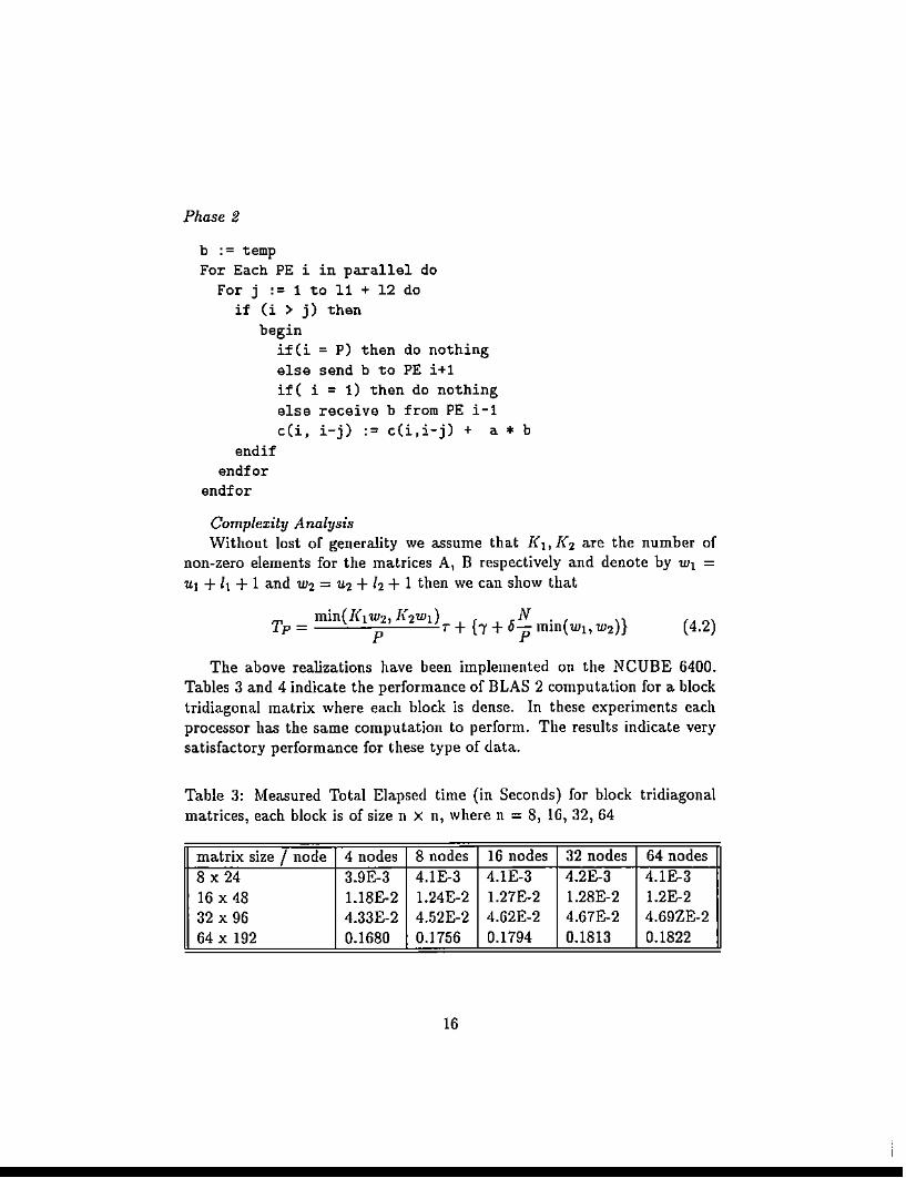
T min(J(,w" [('w,) { ,N. ( )}p= P T+ i+ U p mm WI,W2 (4.2)
The above realizations have been implemented on the NCUBE 6400.Tables 3 and 4 indicate the performance of BLAS 2 computation for a blocktridiagonal matrix where each block is dense. In these experiments eachprocessor has the same computation to perform. The results indicate verysatisfactory performance for these type of data.
Table 3: Measured Total Elapsed time (in Seconds) for block tridiagonalmatrices, each block is of size n X n, where n = 8, 16,32,64
In this section, we make an attempt to formulate the neural nets includedin Figure 1 in a matrix-vector form. For this presentation, we have adoptedthe notation and description adopted in [HNC gO).
4.1 Hopfield Net (HOP)
The HopfLeld network has been useful in performing content-addressable recall and solving optimization problems. A standard Hopfield network consists of two processing slabs (slab = groups of PEs with the same processingequations. A slab can be viewed as a layer). Following [HNC 90] description,we will divide each Hopfield PE into two components (U and V) resulting in3 slabs, where the first slab is the bias slab (I). Next we describe the processing equations based on various numerical differentiation rules. Throughoutwe make an attempt to use a matrix vector formulation of these equations.
4.1.1 Euler processing equations
UOld unew,1T
UoT
fl'V9
neural net input vectors to PEsbias vectorweight matrix where T, is the weight associated with the jth input to the ith HopfieldPEeffective steepness parameterdecay constanttime incrementoutput vector from PEsactivation function
17
The equations and steps used to determine the output of Hopfield PEs are
i) Input T, .6.t, T, UO, 7
ii) Initialization of U01d •
iii) Iterate to compute v = (g(ui/uo».iv) Iterate to compute U new = Uold + .6.t(TV + I - Uold/T)
4.1.2 Runge-Kutta processing equations
In this case the equations and steps used to determine the output of HopfieldPEs are:
From manual "Description, features, applications and network structure".
Processing Equations
Let's denote for fth hidden or output slab:
Nt Number of neurons;
(it The input vector;
1_,
External bias;
Wi Weight matrix between e- 1 and eslabs;
WO Weight matrix between input and output slabs;
Y-t -0The output vector which for input slab it's denoted by V .
Also, throughout we denote by
a = (ai)(a)iaxbnobA'
vector of elemen ts aj
the element i of vector athe cross productthe inner producttranspose of matrix A.
The processing equations and steps that implement the functionality of thenetwork aTe:
i) Input vector for neurons in slab e
where c = 1 if slab eis the output slab and the connections from theinput slab to the output slab are enabled (wO # 0), otherwise c::; 0
ii) Compute output vector slab e
Y = (g(Ui))
19
iii) Learning rule for the output slab (£ = 0).
b' = (y'(Uf)) x (f - V'),
~w' = ",(b' . (iI'-1 )'l,
and
where
9' The derivative of the activation function,
Oti The learning rate for the eth slab,
t The learning input vector.
iv) Learning rule for the hidden slab.
b' = (g'(U,)) X ((Wl+I)'b'+I),
~W' = ",(b'. (iI'-I)'),
andW~ew = W;ld +6.Wi.
In the implementation of MBPN one of the following two operations areperformed to determine the gradient direction: hatching or smoothing. Theprocessing equations for batching are:
i -i-i-II i~W..w = ",(0 (V )) + ~Wold
W;/d +6.W;ew/count if count = batchsizcW:/d otherwise
The processing equations for smoothing are
andWI~ew = W;ld +6.W~ew.
where ilL is the smoothing factor for slab t.
20
4.3 Counter Propagation (CPN)
The outer propagation network is designed to adaptively learn a mappingbetween a set of input and output vectors from examples of the mapping'saction. ePN is useful in solving problems that require the ability to learna mathematical mapping by adaptation in response to examples of correctmappings.
Network Structure
This architecture consists of four slabs: the input slab, the training slab, theKohonen slab and the Grossberg slab. The input slab is fully connected tothe Kohonen slab, which in turn is fully connected to the Grossberg slab.An adaptive weight is associated with each input connection for PEs on theKohonen and the Grossberg slabs. In addition, each Grossberg PE receivesone input from its corresponding training slab PE. This input is used onlyduring training and has no associated weight.
Processing Equations
The equations below are used to update the ePN PE states and weights.The following definitions are used in the discussion:
21
N = Number of Kohonen PEs;
n Number of input PEs;
m = Number of output PEs;
x PE values of the input slab (Xl ••• ", X n );
'ii PE values of the training slab (YI, ... , Yrn);
Z PE values of the Kohonen slab (ZI •.•. , ZN);
'ii' PE values of the Grossberg slab (YI,'" I Ym);
Wi Weight vector of the ith Kohonen PE (Wil, ... , Win);
Uj Weight vector of the jth Grossberg PE (Ujl, ... ,UjN);
bi Bias for the ith Kohonen PE;
Pi = Win frequency for the ith Kohonen PE.
Step 1
Processing for the Kohonen slab begins with calculating the Euclidean distance between the input vector x and each Kohonen weight vector Wi
di =11 Wi -" 11= V(Wi - x)+ (Wi - xl·
Step 2
After d; is calculated, subsequent Kohonen processing depends on whethertraining is enabled. If training is on, the PE with the smallest distance isdetermined according to
if i is the smallest integer for whichd; :5 dj for all j = L.Notherwise
22
Step 3
The Grossberg slab then uses Zj to modify its weights. The equations usedon the Grossberg slab are discussed later in this section.
Next, the Kohonen PE distances are adjusted by the bias values to yieldthe biased distances required by the conscience mechanism. This is doneaccording to
Step 4
ddi - b;
if Win FrequencYi < Tif Win FrequencYi ~ T.
The biased distances are then used to determine which PE will modify itsweight vector. The selection of the biased winner is according to
if i is the smallest integer for which d~ ~ dj for all j = 1otherwise
Step 5
After the biased winner is selected, the weight vectors are modified accordingto
where c is user determined parameter. ,Thus, as the Kohonen PEs neaT the equiprobable distribution, the con
science mechanism is automatically disabled.
23
Step 7
The actual win frequency for a Kohonen PE is calculated using a fading·window averaging process. This is accomplished by
where b is a user parameter which determines the period over which theaverage is taken.
Step 8
If training is not enabled, the Kohonen output values Vi are determinedaccording to the following equations. These equations define an interpolationmechanism when the parameter Winners is greater than one. Let q equalthe desired number of winners, then define S as
S = (i t ,i2 , ••• ,iq )
where iI, i2, ... ,iq are the Kohonen PE indices such that dill di2,···,di" ~
dj for all j€{{l,2, ... ,N} - 5}. The actual number of winners in Scanbe greater than the desired number jf a tie occurs at diq • In this case allPEs with a distance of di " are accepted, and q is incremented to reflect thenumber of indices in S. The minimum distance must then be selected:
do = min(d j ), i E S.
Using dOl each Kohonen PE output, Zi is calculated as follows:* ifiESanddo#O1 if i E Sand i is the smallest integer
ei = such that d; = do = 0o if i E Sand di '# do = 0o ifiES
fi = efIi
Zj=-N~-
2::'=1 Ij
24
Step 9
The processing equations for the Grossberg slab are much simpler than thosefor the Kohonen slab. The output of the kth Grossberg PE is calculated by:
N
Yk = 'Uk' Z = L Uk;Zj
;=1
where z is a vector containing all the Zj values.If training is enabled, then:
old + ( old ',f'Uk; a Yk - 'Ukiuo1d ifki
Zi = 1Zi = a
or
_.new _ _ old + ~(-l ---aId) X -i -Uj .... Y-u Z
where a: is a network parameter and Yk is the kth element of the trainingvector. Only the Grossberg weights associated with connections from thewinning Kohonen PE (the only one for which Zi = 1) are modified. In thesteady-state solution, this equation becomes:
where AVG(Yk) is the average value of all Yk values present when this weightwas allowed to modify. This average uses an exponentially-decaying timewindow with decay rate determined by the parameter Q.
4.4 Learning Vector Quantization (LVQ)
The LVQ network is applicable to difficult pattern classification problems.Its adaptive capabilities allow it to be used in problems in which there islittle a priori knowledge of the pattern class distributions. It has been usedsuccessfully to classify phonemes derived from continuous speech data.
The HNC version of Learning Vector Quantization to be implementedon parallel machines contains three slabs: the input slab, the Kohonen slab,and the training slab. The input slab is fully connected to the Kohonenslab. An adaptive weight is associated with each input to the Kohonen slabconnections. The Kohonen slab is partitioned into groups of PEs. There isone group for each pattern class. Thus each Kohonen slab PE is assigned
25
to a particular pattern class. The number of PEs per class must be equalfor all classes. The training slab contains one PE that is connected to eachKohonen slab PE. There are no weights associated with these connections.This training slab PE must contain the right class number of the inputpattern vector.
Processing Equations
Step 1
The standard LVQ training mode begins with a calculation of the distancedi, between each Kohonen PE's weight vector Wi and the i input vector xaccording to
"di =11 Wi -" 11= 2)Wi; - x;)'
j=l
where n is the size of the input vector.
Step 2
The PE with the smallest distance is designated the network-wide winner.With conscience disabled, this PE adjusts its weight vector according to
if the network-wide winneris in correct classif the lletwork-wide winneris in incorrect class
where Ct and "Yare the user-selected learning rates and the index q designatesthe network-wide winner. This equation moves the network-wide winner'sweight vector a small distance toward or away from the input vector alongthe line joining the current weight vector and the input vector.
Step 3
When conscience is enabled, the PEs assigned to the correct class (i.e., theclass associated with the input vector) have their distances adjusted by abias term according to the following equations:
26
where c is a user parameter, N is the number of Kohonen PEs per class,and p; is the relative win frequency for the ith PE. The win frequencies arecalculated among the PEs assigned to a class; they are not network-wide.
Step 4
The biased distances are then used to calculate the in-class winner. If theindices q and s are used to designate the network-wide and in-class winnersrespectively, the weight vectors of these two PEs are adjusted according to
-oldW, if network-wide winner is in
the correct classif network-wide winner is notin correct class
if in-class winner is inthe correct classif in-class winner is notin correct class
where f3 is a user selected learning rate. The network-wide and in-classwinners may be the same PE, in which case the weight vector is adjustedby the a factor.
Step 5
The win frequencies for each PE are calculated using a fading-window average. The equation for this is given by
{P,,, + b( 1 0 -1"")new I • I
Pi = pfld + b(O.O - pfld)
4.5 Adaptive Ring
if PE i is the in-class winnerif PE i is not the in-class winner
The adaptive ring network is suitable for optimization problems involvingconflict between a mapping constraint and a topological constraint. For example, in the traveling salesman problem the requirement that the salesmanvisit every city forms the mapping constraint, and the requirement that thetour be a closed circuit of minimum length forms the topological constraint.
27
The adaptive ring neurosoftware can also operate in a disconnectedmode, in which the connections between PEs are removed and the PEs areallowed to adapt independently. In this mode the network can be used toimplement vector quantification and functions as a nearest-neighbor lookuptable. In this mode, the adaptive ring network is similar to ePN, with thenotable differences that there is no processing on the output layer as in ePN.Instead, the weights of the winning PE are mapped directly onto the outputlayer.
The adaptive ring network is a four-slab network that works as a singlelayer. The slabs include an input slab, a Kohonen slab, a competition slaband a boundary slab. The input slab is used to pass data to the Kohonenslab. It is fully connected to all Kohonen slab PEs. The Kohonen slab isa closed loop of Kohonen PEs with each PE connected to its two nearestneighbors. Each PE is also connected to the competition slab. The singlePE competition slab polls the Kohonen PEs and determines which is closestto the input vector. The boundary slab allows a subset of the Kohonenslab PEs to be identified as "boundary" PEs. Such PEs do not adjust theirweights as training progresses.
Processing Equations
Step 1
An input vector Y k is selected according to the PDE (Probability DensityFunction) that is being mapped. The Kohonen slab PE with the closestweight vector Xi is determined based on the reduced distance
( K)dk; =lIih - x; II P; + N
where If is a user-selected parameter and Pi is the win frequency for thejth Kobonen PE. If J( is 0, then the actual distance between YiN and Xi isadjusted by the relative win frequency only. As Pi decreases dki increases.This allows PEs that are not winning very often to win, thereby forcing allKohonen slab PEs to participate in the PDE mapping. Since 0 :::; Pi :::; 1 alarge value of [( will disable the attention mechanism.
Step 2
The relative win frequency estimate Pi is calculated using a fading windowaveraging process according to
28
l:!.. . = { b(l- Pi) if the jth PE is the winnerPl b(O - Pi) otherwise
p~ew = Pjld + 6.Pj
where b determines the size of the fading window.
Step 3
The distance metric used has the following form
II Yi - xi 11= 2:)Y;, - xi')"
•where n is a user-selected parameter. In most applications, n is set to 1(Manhattan matrix) or w (Euclidean metric).
Step 4
Finally the weight vector Xj of the winning PE is adjusted according to thelearning law
D.Xj = O:("Yk - Xj){1j
X,!-fW = :t?/d + 6.-X'J , J
where Q' is the learning rate for the winnind PE. The term {3j is the value ofthe boundary slab input signal for this PE if the boundary slab is enabled.Otherwise Bj is set to 1 for all Kohonen slab PEs.
The weight vectors of the PEs that neighbor the winner are also adjusted.These weights aTe either adjusted toward the input vector or the weightvector of the winning PE. The run-time flag WinMap determines which isused. The updating of these weight vectors are given by
';Xi = {{3(Xi - xi)Bi{3(y. - x;)B;
if WinMapif WinMap
= 1=0
29
where f3 is the learning rate for the neighbors of the winning PE and i ;;; j±1.The value of f3 is reduced as training progresses by multiplying it by a coolingfactor after each iteration of the network.
4.6 Bi-directional Associative Memory (BAM)
The BAM network can be used to solve pattern recognition problems ina noisy environment and other applications where content addressability isimportant. BAM is a feedback neural network, which works as a singlefunctional layer. This layer is divided into two slabs, referred to as the Xslab and the Y slab. The X slab is fully connected to the Y slab, and theY slab is fully connected to the X slab.
Processing Equations
Step 1
Each BAM PE has a state value of either lor-I. When learning is disabled,Y slab PEs update their state values according to the equation:
{
I if I::ix WjjXi > 0Y'rw
;;; it'd if I::ix WjiXi ;;; 0-1 if I::ix WjiXj < 0
where Yi is the state value of the jth slab PE, Xi is the state value of theith X slab PE, Wi; is the weight associated with the connection to the jthY slab PE from the ith X SLAB PE, AND cX is the size of the X slab.
Similarly, X slab PEs update their state values according to the equation:
{
I if D Y"j'Y' > 0
x,!-ew ;;; x,!/d if ",,?Y v ..y. ;;; 0J J L...l J"
-1 if I::iY CiiYi < 0
where Uij is the weight associated with the connection to the ith X slab PEfrom the jth Y slab PE and cY is the size of the Y slab.
One iteration of the BAM network with learning disabled consists of a Yslab update, followed by an X slab update in accordance with the equationslisted above. Typically the network is iterated until the X and Y state valuesdo not change from one iteration to the next. This convergence is guaranteedto occur if the matrix W, made up of the weights wi'- is the transpose of thematrix V, composed of weights U;j. In other words, convergence occurs ifWii ;;; uii for every i and j.
30
Step 2
When learning is enabled, the weights are updated according to an outerproduct rule. Using this rule, L associations {(Xl, Yd (X2•Y2), ... , (XL. YL)}where Xk and YI.: are column vectors are stored as follows:
andL
v=I:x/,:yl·k
In other words,L
Wi; ;; LY/.:jXzik
andL
Vij = Wj; L WkjXki.
k
One term in the sums given above is calculated on each iteration of theBAM when learlling is enabled. The current state values in the X and Yslabs are nsed in the calculation. To create the weight matrices Wand V,the user should load each pair of associated vectors into the X and Y slabsand iterate the BAM once per pair.
The number of associations that can be stored with this simple learning technique is quite small and can he expected to be mucn less thanmin(cX,cY).
4.7 Adaptive Resonance Theory 1 (ARTl)
The adaptive resonance architecture provides pattern recognition where thesequence of input vectors is arbitrary, but continuous. As the values arepresented, the network responds in real time with stable, self-organized pattern recognition codes. During recognition, the network matches invariantproperties in the input pattern with exemplars in a recognition category.Thus learning is stable and adaptive, and can be buffered against noise andother irrelevant input.
ARTl is a feedback network that can be used in applications where theinput noise level is very low so the binary patterns can be perfectly learned
31
and/or classified. This includes applications where the exact nature of thepatterns may not be known in advance and the input noise level is very low.
The HNC implementation of ARTI is a two-layer neural network withfour slabs.
The four slabs used to implement ARTI are FO, FI, F2 and F3. TheFO slab is the input slab. It is connected one-to-one with the FI slab. Theshort-term memory (STM) slabs Fl and F2 are used to store activationpatterns and generated responds. They communicate with each other viatop·down and bottom-up connections. FI is fully connected with F2 and F2is fully connected with Fl. A set of adaptive weights is associated with boththe top-down and the bottom-up connections. These weights implement thelong-term memory (LTM) of the network. Slab F3 is a state slab that doesno learning or network processing. FO and FI are Boolean (integer) arrays,F2 is a trivalent array, and F3 is a two-element array.
Processing Equations
The ART I processing equations are simplified versions of the complete adaptive resonance theory equation set.
The following index sets are used throughout this section:
I All active FO PEsj
v(j) All FI PEs with top-down weights from the jth F2 PE over the criticallevelj
X AU PI PEs that are currently active;
J All F2 PEs that are not inhibited for a given input pattern.
The input pattern is a binary vector with each element Ii defined as
[. _ { Active• - Inactive
if i E Iotherwise
The output of each FI slab PE is given by
{Active
x' -I - Inactive
32
ifi E Xotherwise
if T j = max{Tk : k E J}otherwise
where X is defined as
{I if all F2 PEs are inactive
X = In v(i) if the jth F2 PE is active
Only one F2 PE is active at any given time. The output states of the F2slab PEs are given by
{Active
Yj = Inactive
where Tj is
Tj= LWjj.ieX
A reset of the F2 slab active PE occurs if the ratio of active Fl PEs to activeFO PEs is less than the user-selected vigilance parameter V. The vigilanceparameter should lie between a and 1 inclusive. Reset occurs if
IIInv(i)1III III < V
where the magnitude of an index set is defined as the number of indices inthe set_
If learning is enabled, the weights of the Fl and F2 slabs are modifiedwhen resonance occurs. The ARTl package implements the fast learningform of the weight modification equations. These are given by
{L ifiEX
x .. - I 1+11"11IJ - 0
{I ifiEX
Wji = 0 if i tE,X
wnere j is the index of the active F2 PE and i is the index of an FI PE.An important part of the processing equations of ARTI is the initial
values of the top-down and bottom-up weights. If these weights are not setto the proper initial values, the network will not function correctly.
The initial weight values must satisfy the following conditions:
LO<Wij < L l+M
8, - 1D
1< Wj; < 1
where M is number of FI PEs and B} and D1 are user-selected parameters.
33
5 Performance Evaluation of Parallel ANN
In this section we present some preliminary results of the performance ofVML based implementation of HOP and MBPN networks on the nCUBEand Intel IPSC/2 (i860) parallel machines. The VML primitives used havebeen appropriately mapped to these machines. The HOP net consideredwas applied to solve the mapping of certain computations to MIMD parallelmachines. This mapping is formulated at the geocometricjtopological data(grids or meshes) of the computations [HOllS 91] as an optimization problem.The objective of the mapping strategy realized through a HOP net is tosul:ldivide a grid or mesh in P (number of processors) subdomains that haveminimum interface length and equal number of grid points or elements. Forthe results presented here, we have considered a HOP llet for the 2-waypartitioning of an orthogonal N x N grid of an orthogonal region. First inTable 5, we present the total sequential time of three different processors.
Total Execution Time (Sec)Connectionsper iteration nCUBE II i860 Sun 4/470
Table 5. The execution time of a Hopfield net for the 2-way partitioning of8 x 8, 16 x 16 and 32 x 32 grids.
Notice that the times for i860 are for scalar code. We intend to repeatthese experiments in vector mode. In Table G we present the best execution time obtained for the above partitionings in two hypercube parallelmachines, nCUBE II and Intel IPSCj2 based on i860. The Intel machine toour disposal has only 16 processors.
34
Best Total Time in SecConnections nCUBE IPSC/2per iteration Time Processors Time Processors
8' 5.0 8 .7 816' 7.2 16 4.5 1632' 31.4 64 60.2 16
Table 6. The HOP net numerical simulation time and machine configurations used for obtaining 2-way partitionings of 8 x 8, 16 x 16, and 32 x 32orthogonal grids on the nCUBE and Intel IPSC/2.
It appears that the Intel time for a 2-way partitioning of 32 x 32 can beimproved if additional processors were available. For the benchmarking ofparallel computers two additional indicators are usually computed. Theseare the fixed speedup (S = TIITp) and the corresponding efficiency (e =SIP). Tables 7 and 8 present values for these indicators for Intel machineand the 2-way partitioning of 8 x 8, 16 x 16, and 32 X 32 grids using a HOPnet.
Table 8. The fixed speedups and corresponding efficiency for three 2·waygrid partitionings obtained by a HOP net in nCUBE II.
For the benchmarking of neurocomputers, two additional measures are usu·ally computed. These are MCPS (Million Connections Per Second) andMCUPS (Million Connections Updated Per Second). In Table 9, we list theMCUPS obtained by the three machines used so far. In the case of HOPnet for the grid partitioning application, the
CUPS = (number of iterations)*( N 4 jtime)
where N x N is the size of the grid to be partitioned.
MCUPSGrid size nCUBE iPSC/2 Sun 4/470
8x8 .122 .87 .0116 X 16 1.1 1.8 .0532 X 32 4.0 2.2 .07
Table 9. The machine performance measured in MCUPS for three 2-waygrid partitionings obtained by a HOP net.
The above results indicate that the Hopfield net numerical simulation, canbe significantly speeded up by general purpose multiprocessors. In fact, wehave observed close to optimal performance for large nets. It is worth notingthat in all computations floating point arithmetic was used.
36
To test the performance of the VML based implementation of MBPNnetwork, we considered a three layer BPM net and a very simple application. All the performance indicators presented in the previous tables werecomputed for this case too. The input of this application is a single vector ofsize N. Table 10 gives the fixed speedups and efficiences for three differentsizes of input vectors on the nGUBE II.
Table 10. The speedups and efficiencies of parallel MBPN for three dlfferentsize input data on the nGURE.
Here we observed that the speedups obtained are far from optimal. It isworth noticing that there are many alternatives for parallelizing the MBPNnet other than the VML approach. Table 11 presents the best times onthree machines to achieve 10-1 matching with a priori defined output.
Best total time in secondsinput size nCUBE Sun 4f470 Sun IPC
Table 11. The performance of nCUBE, iPSGj2 and Sun IPe for MBPNcomputations.
37
6 References
[Aboe 89] M. Aboelaze, Unpublished Manuscript, June, 1989.
[Ahoe 91] M. Aboelaze, N. P. Chrisochoides, E. N. Houstis and C. E.Houstis. The Parallelization of Level 2 and 3 BLAS Operations onDistributed Memory Machines, Proceedings of First Austrian Conference on Parallel Computing, September 1991.
[Bern 89] J. Berntsen Communication Efficient Matrix Multiplication onHypercubes, Parallel Computing, Vol 12, No 3, Dec. 1989 pp. 335-342
[Bakh 90] S. H. Bokhari Communication Overhead on the Intel iPSe-SGOHypercube. leASE Interim report 10, NASA Langley Research Center, Hampton, Virginia 23665.
[Cher 88J V. Cherakasky and R. Smith, Efficient Mapping and Implementation of Matrix Algorithms on a Hypercube, The Journal of Supercomputing, Vol 2, pp. 7-27,1988.
[Chri 90] N. P. Chrisochoides, Communication Overhead on the NCUBE6400 Hypercube. Unpublished manuscript, December 1990.
[Deke 81] E. Dekel, D. Nassimi, and S. Salmi, Parallel Matrix and GraphAlgorithms, SIAM Computing, Nov. 1981, pp. 657-675.
[Fox 87J G. C.Fox, S. W. Otto, and A. J. Hey, Matrix Algorithms on aHypercube I : Matrix Multiplication, Parallel Computing, 1987, pp.1731.
[Gare 79] M. R. Garey and D.. Johnson Computers and Intractability, AGuide to the Theory of NP-Completeness.
[Hous 91] E. N. Houstis, H. Byun and S. K. Kortesis, A Workload Partitioning Strategy for Scientific Computations by Generalized NeuralNetworks, Proceedings of International Joint Conference on NeuralNetworks, IEEE, July 1991, to appear.
[John 85] S. L. Johnsson, Communication Efficient Basic Linear AlgebraComputations on Hypercube Architecture, Technical Report YALEjCSDjRR361, Dept. of Computer Science, Yale University, 1985.
38
[John 89J S. 1. Johnsson, T. Harris, and Kapil K. Mathur, Matrix Multiplication on the Connection Machine, Proc. Supercomputing 89, Nov.13-17 1989, Reno Nevada, ACM Press, pp. 326-332.
[Kung 82J H. T. Kung, Why Systolic Architecture, Computer, Vol 15, No1, Jan. 1982, pp. 37-46.
[Mira 84) W. 1. Miranker and A. Winkler, Space-Time Representations ofComputational Structures, Computing, Vol. 32,1984, pp. 93-114.
[Mold 82J D. J. Moldovan, On the Analysis and Synthesis of VLSI Algorithms, Trans. on Computers, Vol. C-31, No 11, Nov. 1982, pp.1121-1126.