A Volume Mesh Finite Element Method for PDEs on Surfaces Maxim A. Olshanskii 1 , Arnold Reusken 2 , and Xianmin Xu 2,3 Bericht Nr. 342 Juni 2012 Keywords: surface finite element, surface SUPG stabilization, residual–type surface finite element error indicator AMS Subject Classifications: 58J32, 65N30 Institut f¨ ur Geometrie und Praktische Mathematik RWTH Aachen Templergraben 55, D–52056 Aachen (Germany) 1 Department of Mechanics and Mathematics, Moscow State University, Moscow 119899, Russia e-mail: [email protected]2 Institut f¨ ur Geometrie und Praktische Mathematik, RWTH Aachen University, D–52056 Aachen, Germany e-mail: {reusken, xu}@igpm.rwth-aachen.de 3 LSEC, Institute of Computational Mathematics and Scientific/ Engineering Computing, NCMIS, AMSS, Chinese Academy of Sciences, Beijing 100190, China
Abstract. We treat a surface finite element method that is based on the trace of a standard finiteelement space on a tetrahedral triangulation of an outer domain that contains a stationary 2Dsurface. This surface FEM is used to discretize partial differential equation on the surface.We demonstrate the performance of this method for stationary and time-dependent diffusionequations. For the stationary case, results of an adaptive method based on a surface residual-type error indicator are presented. Furthermore, for the advection-dominated case a SUPGstabilization is introduced. The topic of finite element stabilization for advection-dominatedsurface transport equations has not been addressed in the literature so far.
Maxim A. Olshanskii, Arnold Reusken, and Xianmin Xu
1 INTRODUCTION
Moving hypersurfaces and interfaces appear in many physical processes, for example in mul-tiphase flows and flows with free surfaces. Certain mathematical models involve elliptic partialdifferential equations posed on such surfaces. This happens, for example, in multiphase fluids ifone takes so-called surface active agents (surfactants) into account [1]. In mathematical modelssurface equations are often coupled with other equations that are formulated in a (fixed) domainwhich contains the surface. In such a setting, a common approach is to use a splitting schemethat allows to solve at each time step a sequence of simpler (decoupled) equations. Doing so onehas to solve numerically at each time step an elliptic type of equation on a surface. The surfacemay vary from one time step to another and usually only some discrete approximation of thesurface is available. A well-known finite element method for solving elliptic equations on sur-faces, initiated by the paper [2], consists of approximating the surface by a piecewise polygonalsurface and using a finite element space on a triangulation of this discrete surface. This approachhas been analyzed and extended in several directions in a series of papers, e.g. [3, 4, 5, 6, 7, 8].Another approach has recently been introduced in [9]. The method in that paper applies to casesin which the surface is given implicitly by some level set function and the key idea is to solvethe partial differential equation on a narrow band around the surface. Unfitted finite elementspaces on this narrow band are used for discretization. Yet another method has been studiedin [10]. The main idea of the method in the latter paper to use time-independent finite elementspaces that are induced by triangulations of an “outer” domain to discretize the partial differ-ential equation on the surface. The method is particularly suitable for problems in which thesurface is given implicitly by a level set or VOF function and in which there is a coupling witha flow problem in a fixed outer domain. If in such problems one uses finite element techniquesfor the discetization of the flow equations in the outer domain, this setting immediately resultsin an easy way to implement discretization method for the surface equation. The approach doesnot require additional surface elements. If the surface varies in time, one has to recompute thesurface stiffness matrix using the same data structures each time. Moreover, quadrature routinesthat are needed for these computations are often available already, since they are needed in othersurface related calculations, for example surface tension forces. Opposite to the method in [9]the method from [10] does not use an extension of the surface partial differential equation butinstead uses a restriction of the outer finite element spaces. This method has been further inves-tigated in [11, 12]. In the paper [12] a posteriori error indicators for this surface finite elementmethod are introduced and analyzed.
In this paper, we reconsider this volume mesh finite element method. We review the mainideas and results from [10, 12] and illustrate its behavior by presenting results of numericalexperiments for different classes of problems. We restrict ourselves to the case of a stationarysurface. Stationary and time-dependent diffusion (surface heat diffusion) problems are treated.For the stationary case the error indicator from [12] is briefly recalled and its performance fora surface diffusion problem with a nonsmooth solution is demonstrated. A new aspect, that hasnot been studied in the literature so far, is a stabilization for advection-dominated problems. Weintroduce a surface variant of the SUPG stabilization technique and show that this stabilizationperforms well both for stationary and time-dependent advection-dominated surface transportequations.
2
Maxim A. Olshanskii, Arnold Reusken, and Xianmin Xu
2 BASIC IDEA OF THE VOLUME MESH FINITE ELEMENT METHOD
In this section, we explain the basic idea of our finite element method by applying it to aLaplace-Beltrami model problem. Let Ω ⊂ R3 be a bounded polyhedral domain and Γ ⊂ Ω aclosed smooth hyper-surface in R3. Denote by nΓ the unit outward normal vector on Γ. For asufficiently smooth function g : Ω → R, its surface gradient on Γ is defined as
∇Γg = ∇g − (∇g · nΓ)nΓ.
This definition is intrinsic for Γ and does not depend on how g is extended outside Γ. TheLaplace-Beltrami operator on Γ is given by
∆Γg := ∇Γ · ∇Γg.
We consider the Laplace-Beltrami equation
−∆Γu+ c(x)u = f on Γ. (1)
Here c and f are given functions, with c(x) ≥ 0 on Γ. If c is identically zero on Γ we add theconditions
∫Γu ds =
∫Γf ds = 0 to ensure well-posedness.
The corresponding variational formulation is as follows: Find u ∈ V such that∫Γ
∇Γu · ∇Γv ds+
∫Γ
c(x)uv ds =
∫Γ
fv ds ∀v ∈ V, (2)
with
V =
v ∈ H1(Γ) |
∫Γv ds = 0 if c ≡ 0,
H1(Γ) otherwise. (3)
Let Thh>0 be a family of tetrahedral triangulations of the domain Ω. These triangulationsare assumed to be regular, consistent and stable. We assume that for each Th a polygonalapproximation of Γ, denoted by Γh, is given: Γh is a C0,1 surface without boundary and Γh canbe partitioned in planar triangular segments. It is important to note that Γh is not a “triangulationof Γ” in the usual sense (an O(h2) approximation of Γ, consisting of regular triangles). Instead,we (only) assume that Γh is consistent with the outer triangulation Th in the following sense.For any tetrahedron ST ∈ Th such that meas2(ST ∩ Γh) > 0 define T = ST ∩ Γh. We assumethat every T ∈ Γh is a planar segment and thus it is either a triangle or a quadrilateral. Eachquadrilateral segment can be divided into two triangles, so we may assume that every T is atriangle. An illustration of such a triangulation is given in Figure 1. The results shown inthis figure are obtained by representing a sphere Γ implicitly by its signed distance function,constructing the piecewise linear nodal interpolation of this distance function on a uniformtetrahedral triangulation Th of Ω and then constructing the zero level of this interpolant.
Let Fh be the set of all triangular segments T , then Γh can be decomposed as
Γh =⋃
T∈Fh
T.
Note that the triangulation Fh is not necessarily regular, i.e. elements from T may have verysmall internal angles and the size of neighboring triangles can vary strongly, cf. Figure 1. IfΓ is represented implicitly as the zero level of a level set function ϕ (e.g., the signed distance
3
Maxim A. Olshanskii, Arnold Reusken, and Xianmin Xu
Figure 1: Approximate interface Γh for an example with a sphere, resulting from a coarse tetrahedral triangulation(left) and after one refinement (right).
function), then the discrete surface Γh can be obtained as the zero level of a piecewise linearfinite element approximation to ϕ.
The surface finite element space is the space of traces on Γh of all piecewise linear con-tinuous functions with respect to the outer triangulation Th. This can be formally defined asfollows. First consider the outer space
Vh := vh ∈ C(Ω) | v|S ∈ P1 ∀ S ∈ Th, (4)
where P1 is the space of polynomials of degree one. Vh induces the following space on Γh:
V Γh := ψh ∈ H1(Γh) | ∃ vh|Sh
∈ Vh s.t. ψh = vh|Γh. (5)
When c ≡ 0, we assume that any function vh from V Γh satisfies
∫Γhvhds = 0. Given the surface
finite element space V Γh , the finite element discretization of (2) is as follows: Find uh ∈ V Γ
h
such that ∫Γh
∇Γhuh · ∇Γh
vhds+
∫Γh
ce(x)uhvhds =
∫Γh
f evhds ∀ vh ∈ V Γh . (6)
Here ce, f e are suitable extensions of c and f from Γ to Γh, for example, by taking constantvalues along normals to Γ.
For the finite element method (6) the following optimal error bounds are derived in [10]:
Here h is the characteristic mesh size of the outer triangulation Th. The result in (7) does notrequire any shape regularity of the surface triangulation Fh.
It is clear that the elements of V Γh depend only on the nodal values of outer finite element
functions in the strip ωh containing Γh:
ωh :=⋃
T∈Fh
ST .
4
Maxim A. Olshanskii, Arnold Reusken, and Xianmin Xu
Therefore, it is natural to represent the solution of (6) as a linear combination of the traces ofouter nodal functions on Γh:
uh =N∑i=1
uiφi|Γh, (8)
where φi are the nodal basis functions from Vh. In (8) only the basis functions correspondingto nodes from ωh are used. In general, the set φi|Γh
, 1 ≤ i ≤ N , is not a basis, but only agenerating system of the space V Γ
h . With the representation in (8) one obtains a linear systemfor the coefficients ui, 1 ≤ i ≤ N :
(A+Mc)u = f , (9)
with A = (aij)1≤i,j≤N , Mc = (mi,j)1≤i,j≤N and f = (fi)1≤i≤N given by
aij =
∫Γh
∇Γhφi · ∇Γh
φjds, mij =
∫Γh
ce(x)φiφjds, fi =
∫Γh
f eφids. i, j = 1, . . . , N.
Properties of the matrices A and Mc for c = 1 were studied in [11]. In particular, it was shownthat the diagonally scaled mass and stiffness matrices have (effective) condition numbers thatscale like O(h−2), where h is the characteristic mesh size for the outer triangulation Th.
To solve a parabolic equation on a stationary surface, one can apply a method of lines, i.e.,combine the finite element method described above with a standard finite difference discretiza-tion in time. As an example, consider the heat equation on the surface:
ut −∆Γu = f on Γ,
with initial condition u|t=0 = u0. The application of the finite element method results in anODE system of the form
M1ut +Au = f , (10)
which can be integrated in time numerically. In our experiments below we apply the Crank-Nicolson method:
M1un+1 − un
δt+
1
2A(un+1 + un) =
1
2(fn+1 + fn). (11)
2.1 Results of numerical experiments
Two numerical examples illustrate the performance of the surface finite element method.
Example 1 The Laplace-Beltrami equation (1) is solved on the unit sphere Γ with
f(x) = 12x1x2x3.
By direct compuation, one checks that
u(x) = x1x2x3
is the solution of (1) for c ≡ 0.We consider a sequence of uniform tetrahedral triangulations of Ω = (−2, 2)3. The discrete
surface Γh is the zero level of the nodal interpolant of the signed distance function to Γ, cf.Figure 1. The dimensions of the resulting surface FE spaces V Γ
h are N = 100, 448, 1864, 7552,30412. The accuracy of the method is monitored by computing the L2 and H1 surface errors,i.e. errL2 = ‖ue − uh‖L2(Γh) and errH1 = ‖ue − uh‖H1(Γh). The convergence plots in thelog-log scale are shown in Figure 2. The results illustrate the optimal order of convergence, aswas predicted by the results in (7).
5
Maxim A. Olshanskii, Arnold Reusken, and Xianmin Xu
2 2.5 3 3.5 4 4.5−3.5
−3
−2.5
−2
−1.5
−1
log(N)
log(
err L2
)
L2−error
2 2.5 3 3.5 4 4.5−2.5
−2
−1.5
−1
−0.5
0
log(N)
log(
err H
1)
H1−error
slope: −1/2slope: −1
Figure 2: The L2 and H1 surface FE errors for Example 1.
Example 2 We consider the time-dependent surface heat equation (2) on the torus
Γ = (x1, x2, x3) | (√x21 + x22 − 1)2 + x23 =
1
16. (12)
We setf = 100χD,
with D = x | |x − (0, 1.25, 0)| < 0.2. This example models the heat diffusion over Γ, if thearea D of the torus is heated with a constant heat generation rate.
We use a tetrahedral triangulation of the domain Ω = (−2, 2)3, which contains the torus. Theresulting trace space V Γ
h has N = 5638 degrees of freedom. For the time step in the method(11) we take δt = 0.05. The numerically computed solutions for t = 0, 0.5, 1.5, 2.5 are shownin Figure 3. One can clearly observe the heat diffusion on the torus.
3 SUPG STABLIZATION FOR ADVECTION-DOMINATED PROBLEMS
Let w : Ω → R3 be a given divergence-free (divw = 0) velocity field in Ω. If the surfaceΓ evolves with a normal velocity w · nΓ, then the conservation of a scalar quantity u with adiffusive flux on Γ(t) leads to the surface PDE:
u+ (divΓw)u− ε∆Γu = 0 on Γ(t), (13)
where u denotes the advective material derivative and ε > 0 is the diffusion coefficient. In[4] the problem (13), combined with an initial condition for u, is shown to be well-posed in asuitable weak sense.
We study the discretization of this PDE on a steady surface. Hence, we assume w · nΓ = 0,i.e. the advection velocity w is everywhere tangential to the stationary surface. The assumptionsw · nΓ = 0 and divw = 0 imply divΓw = 0, and the surface advection-diffusion equationtakes the form:
ut +w · ∇Γu− ε∆Γu = 0 on Γ. (14)
We are interested in a finite element method for the advection-dominated case, i.e., 0 < ε ‖w‖L∞(Γ)|Γ|
12 .
6
Maxim A. Olshanskii, Arnold Reusken, and Xianmin Xu
(a) (b)
(c) (d)
Figure 3: The solutions of Example 2 for t = 0, 0.5, 1.5, 2.5.
We first treat the stationary problem:
−ε∆Γu+w · ∇Γu+ c(x)u = f on Γ, (15)
with c(x) ≥ 0 and f a given source term.We consider a stabilized formulation of SUPG type. For this we introduce the bilinear form
and the functional
ah(u, v) :=ε
∫Γh
∇Γhu · ∇Γh
v ds+
∫Γh
ceuv ds
+1
2
[∫Γh
(we · ∇Γhu)v ds−
∫Γh
(we · ∇Γhv)u ds
]+∑T∈Fh
δT
∫T
(−ε∆Γhu+we · ∇Γh
u+ ceu)we · ∇Γhv ds,
fh(v) :=
∫Γh
f ev ds+∑T∈Fh
δT
∫T
f e(we · ∇Γhv) ds.
(16)
Let hT be the diameter of the tetrahedron ST from the bulk mesh, which contains T , and de-
fine the cell Peclet number PeT :=hT‖we‖L∞(T )
2εand cT = maxx∈T c
e(x). The stabilizationparameters δT are based on the cell Peclet number [13]:
δT =
δ0hT
‖we‖∞,T
if PeT > 1,
δ1h2T
εif PeT ≤ 1,
and δT = minδT , c−1T , (17)
7
Maxim A. Olshanskii, Arnold Reusken, and Xianmin Xu
with some given positive constants δ0, δ1 ≥ 0. The stabilized finite element method for (15)reads: Find uh ∈ V Γ
h such that
ah(uh, vh) = fh(vh) ∀ vh ∈ V Γh . (18)
The time-dependent problem can be treated with a similar approach. The stabilized spatialdiscretization of (14) is as follows:
m(∂tuh, vh)Γh+ ah(uh, vh) = 0, (19)
with
m(∂tuh, vh) :=
∫Γh
∂tuhvh ds+∑T∈Fh
δT
∫T
∂tuh(we · ∇Γh
vh) ds,
ah(u, v) :=ε
∫Γh
∇Γhu · ∇Γh
v ds+1
2
[∫Γh
(we · ∇Γhu)v ds−
∫Γh
(we · ∇Γhv)u ds
]+∑T∈Fh
δT
∫T
(−ε∆Γhu+we · ∇Γh
u)we · ∇Γhv ds.
Note that ah(·, ·) is the same as ah(·, ·) in (16) with c ≡ 0. The resulting system of ordinarydifferential equations can be discretized in time by the Crank-Nicolson along the same lines asin section 2.
An alternative to the skew-symmetric discretization of the advective terms in (16) is the useof the original form of the advective term, leading to the bilinear form
ah(u, v) :=ε
∫Γh
∇Γhu · ∇Γh
v ds+
∫Γh
ceuvds+
∫Γh
(we · ∇Γhu)v ds
+∑T∈Fh
δT
∫T
(−ε∆Γhu+we · ∇Γh
u+ ceu)we · ∇Γhv ds.
(20)
The bilinear forms ah(·, ·) and ah(·, ·) define different discretizations. The relation between thetwo is given by the equality∫
Γh
(we · ∇Γhu)v ds
= −∫Γh
(we · ∇Γhv)u ds−
∫Γh
(divΓhwe)uv ds+
∑E∈Eh
∫E
we · [mE]uv ds, (21)
where Eh is the set of all edges of the surface triangulation Fh and [mE] = m1E +m2
E , with m1E
and m2E the two unit normal vectors to E, tangential to Γh, from the two different sides of E.
Note that the last two terms do not vanish, in general.Concerning the analysis of this SUPG method we note the following. Using divΓw = 0,
w · n = 0 and the fact that the discrete surface Γh is close to Γ (distance O(h2)) one canderive ‖ divΓh
we‖L∞(Γh) ≤ ch and by this the second term on the right-hand side in (21)can be controlled. The last term on the right-hand side in (21) is much more difficult to dealwith. Note that this term does not occur in the plane Eulerian case. The error analysis of thesemethods is a subject of current research and the results will be presented in a forthcoming paper.
8
Maxim A. Olshanskii, Arnold Reusken, and Xianmin Xu
These results show a satisfactory error bounds only for the SUPG stabilization with the skew-symmetric variant, i.e. a bilinear form as in (16). We are not able, yet, to derive satisfactoryerror bounds for the method with the bilinear form as in (20). Numerical experiments indicatethat using the forms ah(·, ·) and ah(·, ·) works equally well, cf. below.
Finally note that in the SUPG discretizations described above the term ∆Γhuh vanishes for
linear finite elements uh ∈ V Γh .
3.1 Results of numerical experiments
We show results of two numerical tests, which demonstrate the performance of the stabilizedmethod.
Example 3 The stationary problem (15) is solved on the unit sphere Γ, with
w(x) = (−x2√
1− x23, x1
√1− x23, 0)
T .
This velocity field w is tangential to the sphere. We set ε = 10−6, c ≡ 0 and consider thesolution
u(x) =1
πarctan
(x3√ε
).
Note that u has a sharp internal layer along the equator of the sphere. The corresponding right-hand side function f is given by
f(x) =4ε3/2(4 + ε)x3π(ε+ 4x23)
2.
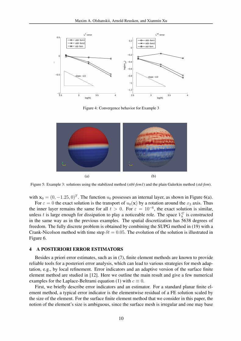
We consider the stabilized method (18) (stbl-fem1), the stabilized method with the alternativebilinear form (20) (stbl-fem2) and the standard finite element method, i.e. δT = 0, (std-fem).The dimensions of the surface finite element space in this experiment are N = 448, 1864, 7552.The resolution is relatively low such that the sharp layers can not be resolved on these meshes.The discretization errors outside the layer are computed: errL2 = ‖u− uh‖L2(D) and errLinf =‖u − uh‖L∞(D), with D = x ∈ Γ : |x3| > 0.3. Results are shown in Figure 4. We observean O(h) error behavior in the L2-norm. In this example we consider an advection-diffusionequation without a zero order term (c ≡ 0). We are not aware of any literature in which this (orany other) convergence behavior follows from a theoretical error analysis.
Figure 5 shows the computed solutions with the stabilized method stbl-fem1 and the usualGalerkin method std-fem. Since the layer is unresolved, the standard finite element method pro-duces globally oscillating solution. The stabilized method gives a much better approximation,although the layer is slightly smeared, as is typical for the SUPG method.
Example 4 This is an example of a time-dependent problem (14) posed on the same torus Γ asin Example 2. We set ε = 10−6 and consider the advection field
w(x) =1√
x21 + x22(−x2, x1, 0)T .
The initial condition is
u0(x) =1
π|x− x0|arctan
(x3√ε
),
9
Maxim A. Olshanskii, Arnold Reusken, and Xianmin Xu
2.5 3 3.5 4−1
−0.5
0
0.5
log(N)
L2
L2−error
stbl−fem1stbl−fem2std−fem
2.5 3 3.5 4
−1.2
−1
−0.8
−0.6
−0.4
−0.2
0
0.2
log(N)
log(
err in
f)
Linf−error
stbl−fem1stbl−fem2std−fem
slope −1/2 slope −1/2
Figure 4: Convergence behavior for Example 3
(a) (b)
Figure 5: Example 3: solutions using the stabilized method (stbl-fem1) and the plain Galerkin method (std-fem).
with x0 = (0,−1.25, 0)T . The function u0 possesses an internal layer, as shown in Figure 6(a).For ε = 0 the exact solution is the transport of u0(x) by a rotation around the x3 axis. Thus
the inner layer remains the same for all t > 0. For ε = 10−6, the exact solution is similar,unless t is large enough for dissipation to play a noticeable role. The space V Γ
h is constructedin the same way as in the previous examples. The spatial discretization has 5638 degrees offreedom. The fully discrete problem is obtained by combining the SUPG method in (19) with aCrank-Nicolson method with time step δt = 0.05. The evolution of the solution is illustrated inFigure 6.
4 A POSTERIORI ERROR ESTIMATORS
Besides a priori error estimates, such as in (7), finite element methods are known to providereliable tools for a posteriori error analysis, which can lead to various strategies for mesh adap-tation, e.g., by local refinement. Error indicators and an adaptive version of the surface finiteelement method are studied in [12]. Here we outline the main result and give a few numericalexamples for the Laplace-Beltrami equation (1) with c ≡ 0.
First, we briefly describe error indicators and an estimator. For a standard planar finite el-ement method, a typical error indicator is the elementwise residual of a FE solution scaled bythe size of the element. For the surface finite element method that we consider in this paper, thenotion of the element’s size is ambiguous, since the surface mesh is irregular and one may base
10
Maxim A. Olshanskii, Arnold Reusken, and Xianmin Xu
(a) (b)
(c) (d)
Figure 6: Example 4: solutions for t = 0, 0.7, 1.4, 2.1.
this notion for an element T ∈ Fh both on the diameter hT of the parent (regular) tetrahedronST and on the area |T | of the surface element. It sometimes occurs that |T | h2T . To accountfor both possibilities, we define a family of residual-type error indicators
ηp(T ) = Cp
(|T |1/2−1/ph
2/pT ‖f e +∆Γh
uh‖L2(T )
+∑E⊂∂T
|E|1/2−1/ph1/pT ‖J∇Γh
uhK‖L2(E)
), p ∈ [2,∞]. (22)
Here uh ∈ V Γh is the finite element solution and E denotes an edge of the element T . When
p = 2, this reduces to the expression η2(T ) = C2(hT‖f e+∆Γhuh‖L2(T )+h
1/2T ‖J∇Γh
uhK‖L2(∂T ))in which the diameter of the outer tetrahedron is used to measure the mesh size. At the otherextreme p = ∞, we have instead the expression η∞(T ) = C∞(|T |1/2‖f e + ∆Γh
uh‖L2(T ) +∑E⊂∂T |E|1/2‖J∇Γh
uhK‖L2(E)) in which the properties of the surface element T are used tomeasure the local mesh size.
The following result (see [12]) shows the reliability up to higher order terms of a posterioriestimators obtained by summing these local indicators over all surface element. Let u and uhbe the solutions to (1) and (6), respectively. For p ∈ [2,∞) the following holds:
‖∇Γ(u− u`h)‖L2(Γ) ≤ C
(∑T∈Fh
ηp(T )2
)1/2
+O(h2). (23)
Here u`h is the lift of the discrete surface functions to Γ. The constant C depends on the shaperegularity of the outer mesh Th and geometric properties of Γ such as curvature. The higherorder term O(h2), where h is the characteristic mesh size of the outer mesh, corresponds to thegeometric errors (resulting from the approximation of Γ by Γh).
11
Maxim A. Olshanskii, Arnold Reusken, and Xianmin Xu
The indicators ηp(T ) can be used to develop strategies for adaptive grid refinement. Nu-merical experiments show that such strategies lead to optimal convergence results for solutionswith local singularities. In the adaptive method, we employ a “maximum” marking strategy inwhich all volume tetrahedra ST from the strip ωh with ηp(T ) > 1
2maxT∈Fh
ηp(T ) are markedfor further refinement.
4.1 Results of numerical experiments
Consider the Laplace-Beltrami equation (1) with c ≡ 0 on the unit sphere. The solution andthe source term in spherical coordinates are given by
u = sinλ θ sinφ, f = (λ2 + λ) sinλ θ sinφ+ (1− λ2) sinλ−2 θ sinφ. (24)
holds. Hence, for λ < 1 the solution u is singular at the north and south poles of the sphere sothat u ∈ H1(Γ), but u /∈ H2(Γ).
We discretize this problem in V Γh using an adaptive method with local refinement based on
the “maximum” marking strategy. For several values of λ the decrease of the error in H1 andL2 norms versus the number of d.o.f. is shown in Figure 7. The results suggest that the errorestimator
(∑T∈Fh
ηp(T )2)1/2 is both reliable and efficient and the performance depends only
mildly on the value of the parameter p.In Figure 8 we illustrate the interface triangulations obtained in the adaptive method. The
results are for the parameter values λ = 0.6 and p = 2. In the left picture we have approximately103 degrees of freedom in the finite element space V Γ
h . The right picture shows the triangulationaround a pole, with a zoom-in factor 20 and a space V Γ
h with approximately 104 degrees offreedom.
5 CONCLUSIONS
We presented an overview of a special finite element method for the discretization of ellipticand parabolic partial differential equations on stationary surfaces. The method uses a polygo-nal surface approximation that is consistent with an outer tetrahedral triangulation of a domainΩ that contains the surface. Such a surface approximation can be obtained in a natural wayin a level set setting. The surface finite element space is defined as the trace of a standard fi-nite element space on the outer tetrahedral triangulation. It has been proved that for diffusiondominated problems the method has optimal order discretization accuracy. This is illustratedby results of numerical experiments. For the diffusion dominated case a residual-type errorindicator has been developed and analyzed. This method is outlined and its behavior illus-trated by numerical experiments. We introduce SUPG type stabilized variants of the methodfor advection-dominated problems. These have not been studied before. The performance ofthese methods is illustrated by results of numerical experiments. Important topics for currentand future research are the theoretical analysis of the SUPG methods and the extension of theseapproaches to problems with partial differential equations on evolving surfaces.
Acknowledgments. This work has been supported in part by the DFG the through grantRE1461/4-1 and the Russian Foundation for the Basic Research through grants 12-01-91330,12-01-00283. We also thank J. Grande for helping us with the implementation of the methods.
12
Maxim A. Olshanskii, Arnold Reusken, and Xianmin Xu
(a) (b)
(c) (d)
Figure 7: Decrease of the error in H1 and L2 norms for different values of λ. The values of the error estimator(∑T∈Fh
ηp(T )2)1/2 are shown. The parameter p equals 2 for figures (a),(c) and (d), while for figure (b) p = ∞.
Figure 8: Interfacial triangulation Γh obtained with adaptive method (left) and zoom in at the pole with the factor20 (right).
REFERENCES
[1] S. Gross and A. Reusken. Numerical Methods for Two-phase Incompressible Flows, vol-ume 40 of Springer Series in Computational Mathematics. Springer, Heidelberg, 2011.
13
Maxim A. Olshanskii, Arnold Reusken, and Xianmin Xu
[2] G. Dziuk. Finite elements for the Beltrami operator on arbitrary surfaces. In S. Hildebrandtand R. Leis, editors, Partial differential equations and calculus of variations, volume 1357of Lecture Notes in Mathematics, pages 142–155. Springer, 1988.
[3] A. Demlow and G. Dziuk. An adaptive finite element method for the Laplace-Beltramioperator on implicitly defined surfaces. SIAM J. Numer. Anal., 45:421–442, 2007.
[4] G. Dziuk and C. Elliott. Finite elements on evolving surfaces. IMA J. Numer. Anal.,27:262–292, 2007.
[5] G. Dziuk and C. Elliott. An Eulerian level set method for partial differential equations onevolving surfaces. Comput. Vis. Sci., 13:17–28, 2008.
[6] G. Dziuk and C. Elliott. Surface finite elements for parabolic equations. J. Comp. Math.,25:385–407, 2007.
[7] G. Dziuk and C. Elliott. Eulerian finite element method for parabolic PDEs on implicitsurfaces. Interfaces and Free Boundaries, 10:119–138, 2008.
[8] G. Dziuk and C. Elliott. L2-estimates for the evolving surface finite element method.SIAM J. Numer. Anal., 2011. to appear.
[9] K. Deckelnick, G. Dziuk, C. Elliott, and C.-J. Heine. An h-narrow band finite elementmethod for elliptic equations on implicit surfaces. IMA Journal of Numerical Analysis,30:351–376, 2010.
[10] M. Olshanskii, A. Reusken, and J. Grande. An Eulerian finite element method for ellipticequations on moving surfaces. SIAM J. Numer. Anal., 47:3339–3358, 2009.
[11] M. Olshanskii and A. Reusken. A finite element method for surface PDEs: matrix prop-erties. Numer. Math., 114:491–520, 2009.
[12] A. Demlow and M.A. Olshanskii. An adaptive surface finite element method based onvolume meshes. SIAM J. Numer. Anal., to appear.
[13] H.-G. Roos, M. Stynes, and L. Tobiska. Numerical Methods for Singularly Perturbed Dif-ferential Equations — Convection-Diffusion and Flow Problems, volume 24 of SpringerSeries in Computational Mathematics. Springer-Verlag, Berlin, second edition, 2008.


![Hunter, P - Finite Element Method & Boundary Element Method [Course Notes 2001]](https://static.documents.pub/doc/80x56/552d570e4a7959c6598b4696/hunter-p-finite-element-method-boundary-element-method-course-notes-2001.jpg)


![Hunter, P - Finite Element Method & Boundary Element Method [Course Notes 2003]](https://static.documents.pub/doc/80x56/55cf9942550346d0339c749a/hunter-p-finite-element-method-boundary-element-method-course-notes-2003.jpg)


