A wavelet approach to the short-term to pluri-decennal ...

INTERNATIONAL JOURNAL OF CLIMATOLOGYInt. J. Climatol. 31: 31–43 (2011)Published online 25 March 2010 in Wiley Online Library(wileyonlinelibrary.com) DOI: 10.1002/joc.1995

A wavelet approach to the short-term to pluri-decennalvariability of streamflow in the Mississippi river basin

from 1934 to 1998

N. Massei,a* B. Laignel,a E. Rosero,b A. Motelay-massei,a J. Deloffre,a Z.-L. Yangb

and A. Rossiaa UMR CNRS 6143 “Continental and Coastal Morphodynamics”, Department of Geology, University of Rouen, 76821 Mont-Saint-Aignan

Cedex, Franceb Department of Geological Sciences, The University of Texas at Austin, 1 University Station #C1100 Austin, TX 78712-0254, USA

ABSTRACT: The temporal variability of streamflow in the Mississippi river basin, including its major tributaries (Missouri,Upper Mississippi, Ohio and Arkansas rivers), was analysed using continuous wavelet methods in order to detect possiblechanges over the past 60 years. Long- to short-term fluctuations were investigated. The results were compared with SOI,PDO and NAO indices and precipitation time series and were also processed by wavelet methods. A major change pointaround 1970, also reported in other works, was recovered in all climate and hydrological processes. It is characterised bythe occurrence of an 8–16-year mode for Upper Mississippi and Missouri and of a 3–6-year mode for all rivers. Two otherdiscontinuities around the mid-1950s and 1985 were also detected. A strong power attenuation of the annual cycle in theArkansas, Upper Mississippi and Missouri rivers was also found between 1955 and 1975. In general, the dominant modesof inter-annual to pluri-annual streamflow variability lay in the 2–4-year, 4–8-year and 10–16-year ranges, which wastypical of SOI for the period of study. A preferential link with the Mississippi basin headwater zone (i.e. Upper Mississippiand Missouri) was deduced during the ≈1934–1950 and ≈1970–1985 periods.

Overall, the contribution of inter-annual to pluri-annual oscillations ranged from 6.6 to 26% of streamflow variance,while the short-term scales (<2–3 weeks) explained from 1.1 to 6.4%. The annual cyclicity explained from 19.1 to 48.6%of streamflow variance. High-frequency streamflow fluctuations linked to synoptic activity were also found to increaseafter 1955 for all basins except Upper and Lower Mississippi, apparently modulated by a ≈2–4-yr oscillation. Copyright 2010 Royal Meteorological Society

KEY WORDS Mississippi; streamflow variability; climate fluctuations; wavelet

Received 5 October 2007; Revised 29 June 2009; Accepted 10 July 2009

1. Introduction

Great rivers’ watersheds play a major role in the worldin terms of water resources. However, the way climateand global environmental changes affect streamflow vari-ability in such basins remains challenging, especially interms of quantification of their respective impact. Ziegleret al. (2005) stated that about 350 years are required todetect plausible changes in the annual streamflow. Yet, itis still possible to attempt the description of changes instreamflow during shorter periods (measurements usuallydo not span more than 100 years).

In the conterminous or in the central United States,many authors investigated the temporal trends of stream-flow variability (Lins and Slack, 1999; McCabe andWolock, 2002). To investigate the temporal trends instreamflow in the United States, Lins and Slack (1999)

* Correspondence to: N. Massei, UMR CNRS 6143 “Continental andCoastal Morphodynamics”, Department of Geology, University ofRouen, 76821 Mont-Saint-Aignan Cedex, France.E-mail: [email protected]

used a methodology based on compilation of quite a largenumber of daily discharge records (i.e. 395 time series)for watersheds relatively free of anthropogenic effects bytrend testing. These authors detected increasing trendsfor most of the US water resource regions for dischargeregimes below the upper quartile (Q75), except on thePacific coast and in some regions of the Southeast, whichexhibited decreasing trends at all quantiles. They con-cluded that the conterminous United States was gettingwetter, but it was less extreme.

Pagano and Garen (2005), in their study of streamflowdata from 141 unregulated basins in the western UnitedStates, reported three different periods of streamflowvariability: (1) a low variability and high persistence(i.e. positive autocorrelation, which means that either dryor wet periods follow each other) between the 1930sand the 1950s, (2) a low variability and anti-persistence(dry periods more often followed by wet periods andconverse) between the 1950s and the 1970s and (3) a highvariability and persistence after the 1980s. After McCabeet al. (2004), 52% of the spatial and temporal variance in

Copyright 2010 Royal Meteorological Society

32 N. MASSEI ET AL.

multi-decadal drought frequency over the United Statesmay be attributed to the PDO and the Atlantic multi-decadal oscillation (AMO), while an additional 22%could be possibly due to general climate warming.

McCabe and Wolock (2002) carried out a study onlarge-scale streamflow variability using the records ofseveral tens of gauges and concluded that there is astep increase in streamflow variability rather than agradual change around 1970. Coulibaly and Burn (2004)also noted striking climate-related features before the1950s and after the 1970s in mean annual streamflowsfrom 79 rivers selected from the Canadian ReferenceHydrometric Basin Network (RHBN) by continuouswavelet transform. This 1970 change point was alsoreported in the study from Anctil and Coulibaly (2004)on the description of the local inter-annual streamflowvariability in southern Quebec, Canada.

Recent works published on the Mississippi basinattempted to predict the potential effects of climatechanges on hydrology (Nijssen et al., 2001; Jha et al.,2004, 2006): for instance, Nijssen et al. (2001), mod-elling water balance changes up to 2045, demonstrated adecrease in snow water storage, resulting in increasedrunoff during the winter, but decreased runoff duringthe snowmelt period. Many significant works used trend-testing statistical methods to detect potential changes inboth amplitude and mean values (Lins and Slack, 1999;Mauget, 2004; Novotny and Stefan, 2007). In other words,these works aim at describing and quantifying potentialtemporal changes in mean and amplitude in streamflow.This addresses the problem of instationarity for whichwavelet-based methods are precisely designed.

In this work, we propose to investigate streamflowvariability in the Mississippi river basin using continuouswavelet analysis. This method had apparently never beenapplied to Mississippi streamflow according to the veryrich literature available. The paper aims at giving a quan-titative overview, statistically speaking, of the respec-tive contribution of long-term potentially climate-relatedoscillations. Two main issues are addressed: (1) the iden-tification of the nature of time-varying characteristicsof long-term fluctuations and the quantification of theirinfluence in streamflow variability and (2) the evolu-tion of short-term fluctuations (1 day to 3 weeks) andtheir potential link to longer-term climate patterns. Dailystreamflow data of some of the major tributaries of the

Mississippi river are used, that is, Missouri, Upper Mis-sissippi, Ohio and Arkansas rivers. These streamflowseries are finally compared with the global Mississippistreamflow series.

2. Hydroclimatological data

2.1. Hydrometeorological time series

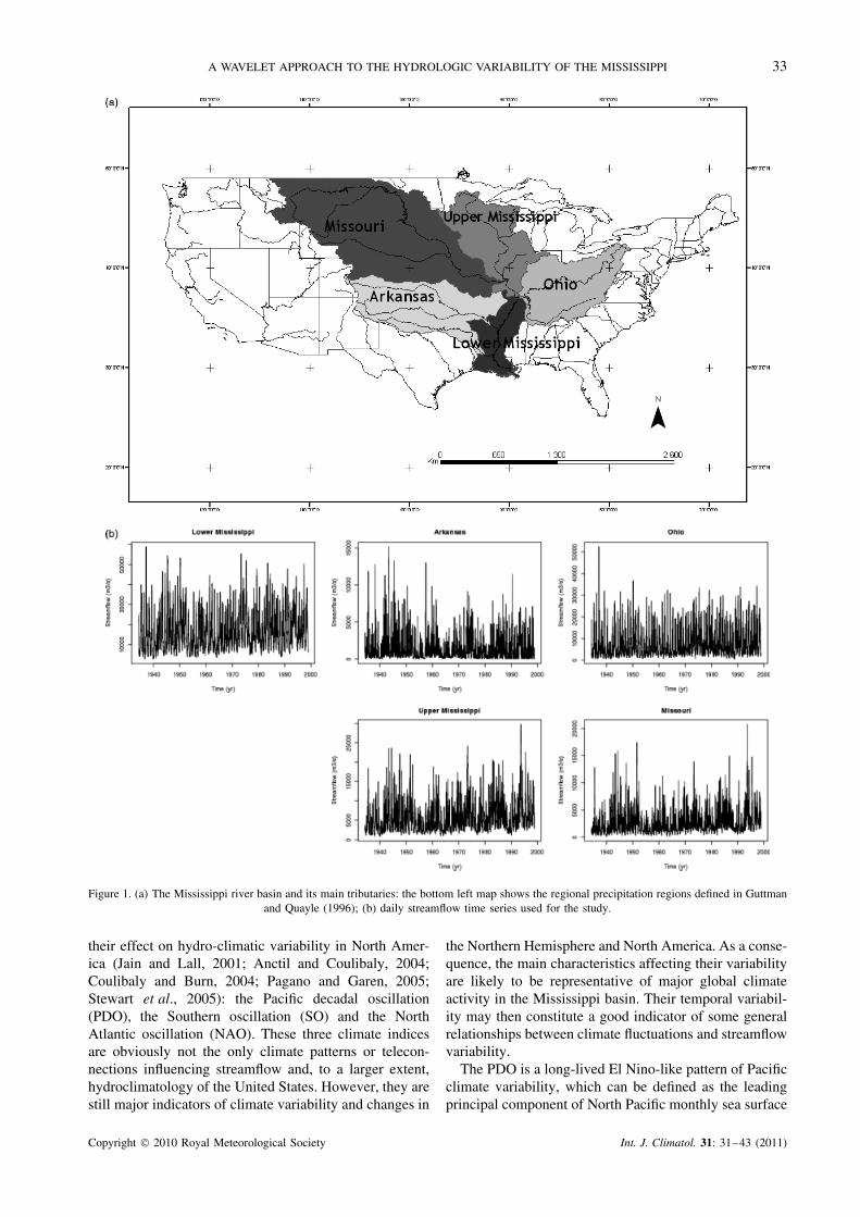
The discharge time series that was used consisted ofdaily streamflow values from the entire Mississippi riverwatershed (referred to as ‘Lower Mississippi’) and someof its most significant sub-basins in terms of dischargecontribution, i.e. Arkansas, Ohio, Upper Mississippi andMissouri Rivers (Figure1a and b). Overall, five dailystreamflow time series were used. Data were obtainedfrom the National Water Information System of the USGeological Survey (http://waterdata.usgs.gov/nwis/sw).All the records used here span a 64-year period from1934 to 1998. Streamflow values were recorded fromstations located at the outlet of the Missouri, UpperMississippi, Ohio and Arkansas Rivers. There werevery few missing values; when existing, blanks wereinterpolated using a cubic spline algorithm. The overallMississippi streamflow time series was also investigated,corresponding to daily values at the outlet of the LowerMississippi. Table I gives the location of stream gaugesalong with the total watershed area for each basin andthe number of large dams when available.

Precipitation variations were also investigated. Theseries that was used consisted of mean annual precip-itation data for climatic regions of the United States(Figure1a) between 1895 and 2000, as defined in Guttmanand Quayle (1996) and provided by the US National Cli-matic Data Center (NCDC). The climatic regions selectedfor data analysis were – according to each basin – theWest North Central, East North Central, Central andSouth regions. An additional mean precipitation serieswas used by averaging over five others to represent pre-cipitation over all five regions. Although this only givesa simplistic representation, it is likely to be sufficient inorder to look at large-scale long-term modes of variabilityin precipitation of annual rainfall in the whole area.

2.2. Climate index time series

Additionally, three monthly climate indices, among majorindicators, were chosen according to the pertinence of

Table I. Stream gauges location and total area and number of large dams for all basins.

LowerMississippi

Arkansas Ohio UpperMississippi

Missouri

Watershed area (km2) 3 202 230 435 122 490 603 489 508 1 331 810Stream gauge location Tarbert+RR

landings(LA)

Murray damnear LittleRock (AR)

Metropolis(IL)

Saint Louis(MO)

Hermann(MO)

Large Dams (WorldResources Institute)

2091 387 711 Unknown 581

Copyright 2010 Royal Meteorological Society Int. J. Climatol. 31: 31–43 (2011)

A WAVELET APPROACH TO THE HYDROLOGIC VARIABILITY OF THE MISSISSIPPI 33

Figure 1. (a) The Mississippi river basin and its main tributaries: the bottom left map shows the regional precipitation regions defined in Guttmanand Quayle (1996); (b) daily streamflow time series used for the study.

their effect on hydro-climatic variability in North Amer-ica (Jain and Lall, 2001; Anctil and Coulibaly, 2004;Coulibaly and Burn, 2004; Pagano and Garen, 2005;Stewart et al., 2005): the Pacific decadal oscillation(PDO), the Southern oscillation (SO) and the NorthAtlantic oscillation (NAO). These three climate indicesare obviously not the only climate patterns or telecon-nections influencing streamflow and, to a larger extent,hydroclimatology of the United States. However, they arestill major indicators of climate variability and changes in

the Northern Hemisphere and North America. As a conse-quence, the main characteristics affecting their variabilityare likely to be representative of major global climateactivity in the Mississippi basin. Their temporal variabil-ity may then constitute a good indicator of some generalrelationships between climate fluctuations and streamflowvariability.

The PDO is a long-lived El Nino-like pattern of Pacificclimate variability, which can be defined as the leadingprincipal component of North Pacific monthly sea surface


34 N. MASSEI ET AL.

temperature variability. As reported in Hanson et al.(2006), a change in the PDO index is a change in thecold and warm water masses of the Pacific Ocean andalters the path of the jet stream that delivers storms to theUnited States. A positive-phase PDO acts to push the jetstream further south into the southwestern United States,while a negative-phase PDO brings the jet stream furthernorth. Therefore, a negative-phase PDO index may leadto less precipitation in the southwest.

The Southern Oscillation index (SOI) is calculatedfrom the monthly or seasonal fluctuations in the air pres-sure difference between Tahiti (T) and Darwin (D) (i.e.mean sea level pressure anomalies T – D). Sustained neg-ative values of the SOI often indicate El Nino episodes;the SOI and El Nino/Southern oscillation (ENSO) are outof phase. During El Nino years/negative SOI, the stormtrack splits more frequently into two preferred branches.The first branch would bring mildly increased storminessin the southern coast of the main part of Alaska. Onthe contrary, the second branch would involve a weak-ening of the storms approaching the Pacific northwestand southwest Canada. In this last case, winter tends tobe wetter than usual from southern California eastwardacross Arizona, southern Nevada and Utah, New Mexicoand into Texas. In the Pacific northwest, El Nino tends tobring drier winters in areas including Washington, Ore-gon and the more mountainous portions of Idaho, westernMontana and northwest Wyoming; these areas correspondwell to the northwestern part of the Missouri River. Inbetween these regions, including central and northernCalifornia, northern Nevada, southern Oregon, northernUtah, southern Wyoming and much of Colorado, theeffects of El Nino are ambiguous. No strong associationcan be discerned in either direction (towards wet or dry).

As described by Hurrell (2000), ‘The NAO refersto a redistribution of atmospheric mass between theArctic and the subtropical Atlantic, and swings fromone phase to another produce large changes in the meanwind speed and direction over the Atlantic, the heatand moisture transport between the Atlantic and theneighboring continents, and the intensity and number ofstorms, their paths, and their weather’. The NAO reflectsthe main fluctuation of climatic conditions in Europeand also affects the eastern/north-eastern coast of NorthAmerica: during positive NAO, these regions as well asnorthern Europe undergo wetter weather conditions andthe converse is true for negative NAO.

The climate index data series can be obtained froma number of climate research centre websites (http://www.cru.uea.ac.uk, http://www.cgd.ucar.edu/cas/jhurrell/indices.htm, http://jisao.washington.edu/pdo/PDO.latest).

3. Methods

Data analysis consisted of Fourier spectral and con-tinuous wavelet analyses. Fourier spectral analysis wasused as a first step to describe the overall behaviourof each time series for the selected 64-year period.

Fourier energy spectra allowed identification of specificbehaviours according to representative time scales, aswell as the comparison of streamflow variability for eachwatershed. Spectra were obtained from autocorrelationfunctions of time series, on which fast Fourier trans-form were performed with application of a Tukey filteringwindow. Fourier spectra were used to compare the hydro-logical behaviour of the sub-basins: for any scaling field,the power or energy spectrum for a given time series hasa power-law dependency on frequency:

E(ω) ∼ ω−β (1)

where ω is the frequency, β the spectral exponent andE(ω) the energy of the spectrum. When plotted withina log–log scale, the energy spectrum displays a linearbehaviour with slope equal to −β. A slope change in thespectrum separates different scaling fields, each relatedto a different hydrologic regime according to time scale.Here, the period (1/ω) is used for the x-axis instead offrequency.

Time–frequency exploration was performed in a sec-ond step using continuous wavelet transform; this methodallows identification of instationarity of the time seriesstudied. This approach has already been successfullyapplied to surface watersheds (Coulibaly and Burn, 2004;Labat et al., 2005). Many published works have alreadypresented the general principle of wavelet analysis (see,for instance, Anctil and Coulibaly, 2004; Labat, 2005),most of which are based on the very accurate presenta-tion of continuous wavelet analysis techniques by Tor-rence and Compo (1998); the reader is referred to theabove-mentioned paper. An even more detailed math-ematical presentation is given in Schneider and Farge(2006). In our study, the Morlet wavelet (a Gaussian-modulated sine wave) was chosen for continuous wavelettransform owing to its good basic frequency resolution;in addition, a wavenumber of 6 was used for the ref-erence mother wavelet resolution, which offered a goodtrade-off between spectral component detection and timelocalisation.

The question often arises about the choice of themother wavelet (What if a different wavenumber/waveletwere chosen? Would the result be the same? etc.).Other wavelets can be used and have been tested toanalyse the present dataset, namely the Paul and DOG(derivative of Gaussian). Depending on the wavelet used,different types of features show up slightly differently.This does not dramatically change the characteristics ofthe spectral content: some features appear more clearlythan others when a given wavelet/wavenumber is used,and the converse is also true. Ideally, several waveletand several basic resolutions of the mother wavelet(wavenumber) should be employed to highlight the moststriking features of a signal and to choose the mostappropriate tool regarding the phenomenon to be analysedand described. For instance, increasing the magnitudeof the wavenumber would result in a better frequencyresolution, in the detriment of time resolution, i.e. the



temporal discontinuities would get ‘blurred’. All thesetests were realised in this study.

The time–frequency diagrams produced give a visuali-sation of the main energy bands present in the time seriesand highlight instationarities, that is, the temporal dis-continuities that may exist in the signal studied. Finally,examination of power fluctuations for either the entirespectral content or selected energy bands is carried outby computing and plotting the so-called scale-averagedcontinuous wavelet spectra. The scale-averaged waveletpower corresponds to the temporal evolution of powerassociated with a selected band of the wavelet spectrum.

4. Scaling regimes of streamflow time series

As a preliminary step to the identification of characteristictime scales and time periods, Fourier spectral analysisis applied to each time series. Table II summarises the

main results that could be obtained from autocorrelationfunctions and corresponding energy spectra (Figure 2).

For all streamflow series, trends (to be removed beforeautocorrelation and Fourier transform) were statisticallytested. All streamflow time series exhibited increasingtrends and the F-statistic provided indication on theincrease rate of each trend. Contrary to what Walling andFang (2003) stated, an increasing trend for the MississippiRiver was found to be statistically significant at the 95%confidence limit (F = 392.4, p < 0.0001 in Table II).

Autocorrelation functions (Figure 2) clearly show thatthe annual cycle is well represented in the series. Indeed,autocorrelation functions display a strong periodicity(gain in correlation) every ∼365 days. However, they alsoreveal different memory effects, which can be representedas a quantitative value characterising the degree of lin-ear correlation for a value with the previous ones. Here,the memory effect is estimated by fitting an exponen-tial decay (y = y0 + a.e−b.t ) to the autocorrelograms. The

Table II. Trends, representative time scales and slopes (exponents) for the different streamflow series over the 64-year(1934–1998) period.

LowerMississippi


Missouri

F-statistic for increasing trend in streamflow 392.4 115.5 228.4 986.2 906.6Memory effect (per day) −2.64 10−2 −2.98 10−2 −2.70 10−2 −2.32 10−2 −2.26 10−2

Breakup time scale (day) 37 15 32 11 14β1 exponent 8.02 6.32 6.13 7.21 7.21β2 exponent 2.08 2.78 1.56 3.04 2.32

All p-values are <0.0001.

Figure 2. Autocorrelation functions and Fourier energy spectra of streamflow time series. Each spectrum displays two different scaling regimesseparated by an 11–37-day time scale, which characterises the difference between short-term behaviour (mainly related to the meteorologicconditions and physiographic features of each basin) and long-term climate patterns. This typical time scale can be related to the so-called

synoptic maximum.


36 N. MASSEI ET AL.

speed at which the fitted exponential decays (expressedin per day) characterises the speed at which informationgets lost in the time series. It constitutes an indicator ofthe global structuration of a time series. The memoryeffect values presented in Table II correspond to the val-ues of parameter b of the exponential. The smaller thevalue of b, the smaller is the memory effect. Arkansas hasthe smallest memory effect, while Missouri displays thelargest one: the Arkansas streamflow series would thenbe poorly structured regarding other watershed series.The reason why the Arkansas streamflow series is lessstructured overall than the others is not clear. Addi-tional research and further investigation would be neededin order to provide consistent hypotheses for this spe-cial behaviour of Arkansas streamflow autocorrelation.In all of the events, the autocorrelation function remainsan interesting tool to get an overview of the generalbehaviour of a signal, although it only provides globalinformation precisely.

Representative time scales and scaling regimes couldbe investigated by Fourier spectral analysis (Figure 2).The spectra display clear breaks separating at least twodistinct flowing regimes. The values of the associatedspectral exponents ß are related to the variability of eachsignal according to time scale: the lower the magnitudeof ß, the higher is the variability in the data, whereashigher ß values correspond to smoother variations. Thetwo different slopes ß1 and ß2 characterise two typesof flow regimes associated respectively with a short-term variability and a long-term variability, respectively.The breakup time scale that separates these two typesof flowing regimes would be related to the typical timescale separating short-term meteorological field fluctu-ations from long-term climate oscillations. The Fourierperiod separating these two domains is known as the syn-optic maximum, the maximum time scale characterisingthe lifetime duration of synoptic events. All energy spec-tra display a 1-year periodicity (the annual cycle) and arecharacterised by distinct ß1 and ß2 values, with slightlydifferent synoptic maxima.

In the long term (ß2 exponent), the Mississippi riversub-basins reveal different behaviours. The Upper Mis-sissippi watershed displays a lower variability (highestß2 exponent) than the other sub-basins. On the con-trary, Ohio is characterised by a higher variability in thelong term (low ß2 exponent of 1.56). In the short term,arranging the various basins according to decreasing ß1gives the following: Lower Mississippi, Missouri/UpperMississippi, Arkansas, Ohio. Arkansas and Ohio presenta high variability (low ß1 exponents), whereas UpperMississippi/Missouri show smoother variations (higherß1). Arkansas displays more contrasted scaling proper-ties between the two long- and short-time scaling regimeswith a low ß1 and a high ß2 exponent. The variabilityin the streamflow is high in the short term, while longertime scales exhibit a lower variability with smoother vari-ations.

It is difficult to distinguish any clear hierarchisationof watersheds according to their scaling exponents. This

might be either due to the small amount of samples(i.e. the five watershed time series used) or due to thestatistical nature of the scaling exponent ß, inasmuch asthe stochastic processes.

5. Fluctuations at annual to pluri-decennal scales

In this section, continuous wavelet transform (Figure 3)is used to investigate the variability of each streamflowseries according to time (i.e. throughout the period ofstudy) and wavelet scale (i.e. from the short term to thelong term). The detected modes of variability are thencompared with those characterising climate indices andprecipitation.

Colours indicate the distribution of power, hereexpressed as normalised decibels (i.e. maximum power =0 db for each scale), with a decreasing power from pur-ple (maximum power) to dark red (minimum power).All series were zero-padded to twice the data length toprevent spectral leakage consequently to wavelet trans-form. However, zero-padding does not prevent from edgeeffects, causing some spectral components to be under-estimated, especially in the lowest frequencies and nearthe edges of the series. The area under the white-dottedcurve on each local wavelet spectrum marks those partsof the spectrum where energy bands are likely to be lesspowerful than they actually are. This area is known asthe cone of influence.

5.1. Main modes of variability and characteristic timescalesSeveral energy bands can be separated on the streamflowlocal wavelet spectra (Figure 3, Table III):

• A 1-year band (annual cycle, A in Figure 3). A strongand obvious attenuation of the intensity – in terms ofvariance – of the annual cycle between approximately1955 and 1975 is observed for all watersheds. Thisphenomenon is less marked for the Lower Mississippiand Ohio Rivers, which reveal a good sustenance ofthe annual cycle power. The annual cycle for ArkansasRiver seems poorly structured and less powerful.

• A 2–4-year band (B), a powerful structure that occursaround 1990 in all streamflow series except OhioRiver, for which this band is barely present.

• A 5–8-year band (C), which seems to be affected bya change towards a 3–6-year band (D) around 1970.

• A 8–16-year band (E) clearly characterises the UpperMississippi and Missouri Rivers, with a powerfulstructure beginning in the early 1970s (around a 10-year Fourier period). This structure is not visible inother streamflow series.

• A last low-frequency 12–16-year band (F) is onlydetected in the Lower Mississippi and Arkansasstreamflow spectra, well localised between 1940 andthe mid-1980s.

Common fluctuations could be recovered for allstreamflow series, while others (for instance, the 8–16-year band E) seemed more specific for some watersheds



Figure 3. Continuous local wavelet spectra of streamflow and climate index time series. The white dotted curves delimit the cone of influence,i.e. the area under which power can be underestimated as a result of edge effects, wraparound effects and zero padding. This figure is available

in colour online at wileyonlinelibrary.com/journal/joc

Table III. Contribution of selected energy bands to total variance of streamflow for all studied basins.

Energy band Streamflow Energy band PDO SOI NAO

A 1 year G 20–26 years – –B 2–4 years C′ 4–8 years 4–8 years –C 5–8 years D′ – 2–8 years –D 3–6 years E′ – 10–16 years –E 8–16 years C′

2 – – 5–7 yearsF 12–16 years E′

2 – – 8–12 years

(typically Upper Mississippi and Missouri). In addition,a shift towards higher frequency fluctuations (Figure 3,in chronologic order: C->D->B) could be observed foralmost all series but Ohio.

In brief, three major patterns show up on the localwavelet spectra (Figure 3):

1. A first discontinuity is visible around 1950–1960: itinvolves a shift from band C to D for Lower Missis-sippi, Arkansas, Upper Mississippi and Missouri and

an interruption of band D for Ohio. It is also accom-panied by a lack of power affecting more specificallythe annual band (A) between approximately 1950 and1975 as described above, and seems more pronouncedfor Arkansas, Upper Mississippi and Missouri.

2. A second discontinuity is visible around 1970 andseems to affect most of the signal components. Itis characterised by the occurrence of a powerful8–16-year band (E) for both Upper Mississippi and


38 N. MASSEI ET AL.

Missouri Rivers, and of a 3–6-year band (D) for allrivers.

3. A third discontinuity can be observed around 1985: theB and D energy bands seem to be more particularlyconcerned by this change, while the lower frequenciesdo not display any striking change. The 3–6-year band(D) would shift quite abruptly towards a 2–4-yearfluctuation (B).

These results seem to be in concordance with thoseof Pagano and Garen (2005), who concluded that thereexist three different periods of streamflow variability intheir analysis of April–September streamflow volumedata from 141 unregulated basins in the western UnitedStates: between the 1930s and the 1950s, the 1950s andthe 1970s and after the 1980s. Similarly, Coulibaly andBurn (2004) reported strong local correlations betweenteleconnection patterns and western, central and easternCanadian streamflows in both 2–3- and 3–6-year bandswith striking changes around 1950 and 1970. Otherauthors, such as McCabe and Wolock (2002), reporteda 1970 discontinuity, which they interpreted as a stepincrease in streamflow in the United States, coincidingwith an increase in precipitation. Overall, these studiesdid not propose any physical mechanisms to explain thephysical influence of climate over streamflow – whichremains extremely difficult.

Wavelet transforms of monthly SOI, PDO and NAOindices were performed in order to compare the scaleand temporal patterns of streamflow with the fluctuationsof three of the major climatic patterns known to impactNorth America (Anctil and Coulibaly, 2004; Coulibalyand Burn, 2004; Hanson et al., 2006). All three indicesare affected by clear temporal discontinuities in theirspectral composition (Figure 3). For the 1930–2000period, the selected climate indices are characterised bythe following modes:

> SOI: before ∼1970, 4–7-year band (C′); after ∼1970,2–6-year (D′) and 11–16-year (E′) bands

> NAO: before ∼1970, 4.5–6.6-year band (C′2); after

∼1970, 8.3–10.6-year band (E′2). NAO is also

characterised by powerful short-term structures;> PDO: it is characterised by a longer-term variability

(19.2–26.3-year band G). A 5.2–7.1-year band(C′) is clearly expressed before ∼1970 anddisappears afterwards.

The time scales of the observed energy bands are givenin Table III along with those detected in streamflow. Amore accurate description of the spectral modes of theseclimate indices can be found in many other works suchas Fernandes et al. (2003), Garcia et al. (2005), Masseiet al. (2007), Coulibaly and Burn (2004), Torrence andCompo (1998), etc.

Local wavelet spectra of annual precipitation timeseries (Figure 4) clearly display very similar featuresthat could be observed in streamflow and climateindices. Major spectral components and discontinuities

are detected such as 8–16-year and 3–6-year bandspresent in West/East North Central precipitation and Mis-souri/Upper Mississippi series, high power at 3–6-yeararound 1950 and between 1975 and 1990 in central pre-cipitation as detected in Ohio streamflow (band D). Thesame ∼1970 discontinuity is observed as well.

5.2. Relation between climate fluctuations andstreamflow instationarity

Some general patterns and changes affecting climateindices are recovered in long-term fluctuations of stream-flow. Although wavelet coherence would undoubtedlyhelp in determining the intensity of correlation betweenthe climatic and streamflow signals analysed, thisapproach was not used here because the time step forstreamflow series and climate indices was basically notthe same (respectively daily and monthly), which wouldhave required streamflow to be downsampled accordingto a monthly time step. However, a detailed study ofwavelet coherence would add some value, especially forthe comparison of streamflow with several (more thanthree, as used in this study) climate indicators.

The change point around 1970 seems to be a con-stant pattern for precipitation, streamflow and climateindex time series. Also, similar energy bands may berecovered (Figures 3 and 4, Table III). This characteris-tic time discontinuity was also reported by other worksin unregulated watersheds (McCabe and Wolock, 2002;Anctil and Coulibaly, 2004; Coulibaly and Burn, 2004),which would then suggest a climatic rather than ananthropogenic origin of such a transient pattern. Here wedemonstrate that this change point is associated with twomajor effects in streamflow according to the watershedconsidered:

1. It involves a shift in the inter- to pluri-annual band(in chronologic order: C, D, B) for Lower Mississippi,Upper Mississippi, Missouri and Arkansas (Figure 3).The (C, D, B) energy bands span the range of scales2–8 years, which is also typical of SOI (Table III).

2. It involves the occurrence of an 8–16-year band (E) inUpper Mississippi and Missouri.

Although the 1970 change point and energy bandD were detected in Ohio streamflow, this watershedis clearly apart from the others in terms of long-terminter-annual to pluri-annual fluctuations. We can alsonotice that it appears rather difficult to relate the powerattenuation over the 1-year band with climate indices orprecipitation variability, although it is particularly wellmarked for Arkansas, Upper Mississippi and Missouri.

SOI in particular appeared to display very similarmodes of variability as those detected in the streamflowtime series, especially in the case of Upper Mississippiand Missouri streamflow (Figure 3, bands E, C, D, Band C′, E′, D′), which deserves particular attention here.A global wavelet spectrum, gathering power across allthe temporal range like a Fourier spectrum, was per-formed on these series to better compare the spectral



Figure 4. Continuous local wavelet spectra of annual precipitation time series. All purple contours are at least 90% significant whentested by the Monte Carlo simulation against a background red noise AR(1) = 0.98. This figure is available in colour online at

wileyonlinelibrary.com/journal/joc

Figure 5. (a) Global wavelet spectra of SOI, Upper Mississippi andMissouri streamflow time series; (b) time-domain reconstructions ofSOI, Upper Mississippi and Missouri streamflow 1.4–16.5-year energy

bands.

components (Figure 5a). Upper Mississippi and Missourispectra display clear similarities with the SOI spectrum

in the frequency range corresponding to the 1.4–16.5-year time scales. A shift in the spectrum towards higherfrequencies is characteristic of a modulation by a high-frequency bearing signal: here it would provide evidenceof a strong influence of SOI on Upper Mississippi andMissouri, i.e. on the Mississippi watershed headwaters inthe 1.4–16.5-year scale range. It is difficult at this pointto draw hypotheses on what physical mechanism wouldbe involved in the filtering of the climate signal in Mis-sissippi headwaters streamflow (atmospheric processes,anthropogenic impact. . .). Although the global waveletspectra revealed a shift in the frequency of the stream-flow in the 1.4–16.5-year band compared to the sameband in SOI, it would be rewarding to compare the cor-responding time-domain bands between streamflow andSO. The purpose of reconstruction is to check for similar-ity between the detected oscillations in SO and in stream-flow (not between the two streamflow series) in terms ofthe expected physical influence: Do negative SOI valuescorrespond to above-normal streamflow for that com-ponent that could possibly link SO and streamflow? Areconstruction of the 1.4–16.5-year band for Upper Mis-sissippi, Missouri streamflow and SOI by inverse wavelettransform (Figure 5b) tend to show an overall good matchbetween SOI and streamflow oscillations for the peri-ods ≈1934–1950 and ≈1970–1985. This is consistentwith the fact that positive ENSO phases (negative SOIphases) are associated with drier conditions in this regionof the United States and the converse is also true. On theother hand, the ≈1950–1970 and ≈1985–1998 periodsare characterised by a poorer correspondence betweenSOI and streamflow, which can be related to the temporalchanges in the spectral composition described previously


40 N. MASSEI ET AL.

in wavelet spectra (Figure 3). In all of the events, furtherphysical interpretations would require many additionalinvestigations.

From a quantitative standpoint, it is interesting toprovide information about the part of variance associ-ated with the various observed time scales. This canbe achieved by wavelet scale averaging. Averaging inscale consists of extracting the power of a given energyband for a time series to either check for power variationthrough time or obtain the variance of the correspond-ing band relating to the total variance of the series. Inour case, the issue to be addressed was the contribu-tion of short-term (inferior to the synoptic maximum),annual and inter-/pluri-annual fluctuations of the totalstreamflow variance. We then computed scale-averagedwavelet spectra (not shown here) over the correspondingenergy bands (Table IV). Three scale-averaged waveletspectra were computed: the first spanning the range ofshort time scales inferior to the synoptic maximum, thesecond corresponding to the annual fluctuation powerand the third corresponding to inter-/pluri-annual fluc-tuations. The time interval chosen for power integrationwas 3 months, which could preserve power variabilityassociated with seasonal fluctuation. Each scale-averagedwavelet spectrum consisted of a 259 point-time series.The part of variance of the different energy bands isexpressed as a percentage of the overall variance ofeach time series. The annual fluctuation obviously rep-resents a large part of total power for each streamflowtime series. However, in the long term, Upper Mis-sissippi and Missouri display a strong power probablyrelated to SOI variations as discussed above, whereasthe overall Mississippi streamflow series (Lower Missis-sippi) and Ohio are definitely dominated by the annualoscillation. The strong power at the annual time scalein the lower Mississippi and Ohio compared to UpperMississippi and Missouri cannot be explained here. Onepotential research track to be explored would concernthe lower number of large dams with respect to the totalbasin area observed for the Missouri River compared tothe others; for instance, the Missouri River comprises581 large dams for an area of 1 331 810 km2, whileOhio comprises 711 for 490 603 km2. An attenuation oflonger-term components, enhancing the variability asso-ciated with the annual cycle, could be a question thatwould require further investigations.

In the short term, Ohio, Arkansas and Missouripresent the strongest contribution of high-frequencyevents compared to Lower and Upper Mississippi (2.9

and 1.1% respectively). Finally, summing the percent-age of variance explained by high-frequency, annual andinter-/pluri-annual fluctuations for each series shows thatArkansas, with less than 40% of variance explained bypowerful well-individualised components, is the morepoorly structured time series, the remaining variancebeing explained by more or less noisy structures in thestreamflow signal.

6. Long-term evolution of short-time flood events

One challenging concern lies in the link between high-frequency/extreme events (rain events, storms, depres-sions and other synoptic events. . .) and long-term vari-ability. Jain and Lall (2001) investigated the potentialimpact of quasi-periodic, inter-annual and inter-decadalvariations in climate (e.g. the ENSO) on flood frequencyand reported a clear control of climate on floods. Inthis section, we try to investigate a possible control oflong-term climate-driven oscillations on the short-termbehaviour of the streamflow time series. In addition, theoverall evolution in the power of high-frequency bandsof streamflow is statistically tested to assess the temporalevolution of flood events over the 64-year period of study.

Scale-averaged wavelet spectra in Figure 6 are pro-duced by scale averaging over the so-called synopticband determined by the Fourier spectral analysis (i.e.the breakup time scale, approximately less than 30 days).The corresponding distribution of variance through timehighlighted a statistically significant increase in the con-tribution of short-term fluctuations for Ohio, Upper Mis-sissippi and Missouri (Figure 6). In order to investigatethe possible modulations of these short-term time scales,that is, inferior to the synoptic maximum, by larger-scaleclimate fluctuations, we proceeded to a smoothing of allscale-averaged spectra using a Savitzky-Golay polyno-mial low-pass filter (Figure 7). This method is based onleast squares polynomial fitting across a moving windowwithin the data. It presents the advantage of preservingthe higher moments in time-domain spectral peak data.The parameters of the filter chosen here were a fourth-order polynomial and a 2-year width smoothing window,which offered the best trade-off between variance con-servation and smoothing.

For all time series, the smoothed scale-averagedwavelet spectra revealed an obvious modulation by largertime scales, in particular by a ≈2–4-year fluctuation(Figure 7). This time scale is typical of some well-known

Table IV. F-statistics and associated p-values for increasing trend of each reconstructed climate-related component.

LowerMississippi


Missouri

% of total variance for time scales < synoptic max. 2.9 4.8 6.4 1.1 4.7% of total variance for annual fluctuation 48.6 19.1 45.3 30.8 19.2% of total variance for inter-annual/pluri-annual fluctuations 11.5 16.0 6.6 25.3 26.0Sum of < synoptic max., annual and inter/pluriannual (%) 63.0 39.9 58.3 57.2 49.9



Figure 6. Scale-averaged wavelet spectra of short-term streamflow fluctuations. The short-term time scale limit was chosen according to Fourierspectra (ß1 scaling exponent), and one seeks possible trends in meteorologic-induced short-time events such as floods. Linear regression models

and slopes are statistically tested by ANOVA (F-statistic) and Student t-test (t-statistic) respectively.

climate indices’ fluctuations such as the SOI/ENSO, asdescribed in Section 5 above, which is known to dis-play a particularly strong power since approximately1960 (Torrence and Compo, 1998). This would suggesta significant control of large-scale climate on the mostrapid fluctuations in streamflow. The discontinuity thatcould be observed on the local wavelet spectra startingaround the mid-1950s (see Section 5.1) was observed onthe smoothed scale-averaged spectra, which was barelyvisible on the initial scale-averaged spectra (Figure 6)except for Arkansas. After this mid-1950s’ discontinu-ity, all smoothed spectra but those of lower and UpperMississippi displayed a statistically significant increasein the power of high-frequency streamflow, which meansthat the contribution in terms of amplitude of short-termevents to the total discharge tends to become greater. Aflood frequency analysis should be conducted addition-ally to test the hypothesis of an associated increase intheir number.

7. Conclusion

In this study, Mississippi and tributaries streamflow serieswere used to investigate long-term to short-term stream-flow variability in relation with climate fluctuations. Twomain issues were initially addressed (1) the identificationof the nature and the temporal characteristics of long-term fluctuations and the quantification of their influencein streamflow variability and (ii) the behaviour of stream-flow regarding short-term fluctuations related to meteoro-logic events (of the order of 15 to 25 days) such as strongfloods: Are they linked to longer-term climate patterns,of what type/nature? Do they present a significant trendthroughout the last 64 years?

All streamflow time series exhibited statistically sig-nificant increasing trends. A major change point wasobserved in streamflow around 1970. This change point,also reported in many other works, would affect mostof the spectral components, and is characterised by theoccurrence of a powerful 8–16-year band for both UpperMississippi and Missouri Rivers, and of a 3–6-year bandfor all rivers. It has been shown that this discontinuity isalso a characteristic pattern of all selected climate indices(SOI, PDO, NAO). Also, a lack of power affectingmore specifically the annual band between approximately1955 and 1975 was detected to be more pronounced forArkansas, Upper Mississippi and Missouri, which wouldoccur almost simultaneously with another temporal dis-continuity starting in the mid-1950s; however, no linkcould be established between these two phenomena. Itmay be rewarding in further investigations to search forpossible links between this 1-year band power attenua-tion and major periods of dam construction. Finally, a lastchange starting around 1985 was detected in streamflowseries. It was difficult to relate the energy bands observedin climate indices and in streamflow, except between SOIand Upper Mississippi and Missouri. For those basins, apotentially strong link was deduced in the 1.4–16.5-yearrange, which appeared rather consistent from a physicalstandpoint after time-domain reconstruction of this modeof variability in each series. A wavelet coherence analy-sis involving climate indices, precipitation and the samestreamflow series, currently carried out as a continuityof this work, will certainly constitute a most appropri-ate approach to the quantification of climate-originatingmodes in streamflow variability.

The contribution of inter-annual to pluri-annual oscil-lations ranged from 6.6 to 26% of the total streamflow


42 N. MASSEI ET AL.

Figure 7. Stavitsky–Golay fourth-order polynomial smoothing of scale-averaged wavelet spectra presented in Figure 4. The smoothing procedurereveals (1) a possible modulation of short-term fluctuations by a quasi-biennal fluctuation (less expressed for Arkansas and Ohio) and (2) a timediscontinuity beginning around about 1953, after which high-frequency streamflow increases significantly and seems to be more controlled by a

quasi-biennal climate fluctuation.

variance. In the short term, i.e. for time scales related tosynoptic activity (>2–3 weeks), high-frequency fluctua-tions explained from 1.1 to 6.4% of the total streamflowvariance. The annual cyclicity was more or less wellexpressed in streamflow variability according to eachwatershed, from 19.1 to 48.6%. High-frequency stream-flow fluctuations linked to synoptic activity were alsofound to increase after 1955 for all basins except UpperMississippi and Lower Mississippi (i.e. the whole Mis-sissippi basin). Finally, a control of short-term stream-flow variations by larger-scale climate fluctuations wasdemonstrated in the form of a modulation by a ≈2–4-year fluctuation.

References

Anctil F, Coulibaly P. 2004. Wavelet analysis of the interannualvariability in southern Quebec streamflow. Journal of Climate 17:163–173.

Coulibaly P, Burn D. 2004. Wavelet analysis of variability in annualCanadian streamflows. Water Resources Research 40: W03105,DOI:10.1029/2003WR002667.

Fernandez I, Hernandez CN, Pacheco JM. 2003. Is the North AtlanticOscillation just a pink noise? Physica A 323: 705–714.

Garcia NO, Gimeno L, De La Torre L, Nieto R, Anem JA. 2005. NorthAtlantic Oscillation (NAO) and precipitation in Galicia (Spain).Atmosfera 1: 25–32.

Guttman NB, Quayle RG. 1996. A historical perspective of U.S.climate divisions. Bulletin of the American Meteorological Society77(2): 293–303.

Hanson RT, Dettinger MD, Newhouse MW. 2006. Relations betweenclimatic variability and hydrologic time series from four alluvialbasins across the southwestern United States. Hydrogeology Journal14(7): 1122–1146, DOI:10.1007/s10040-006-0067-7.

Hurrell J, Kushnir Y, Ottersen G, Visbeck M. 2003. The North AtlanticOscillation: Climatic Significance and Environmental Impact.Geophysical monograph (American Geophysical Union) 134: 1–35.

Jain S, Lall U. 2001. Floods in a changing climate: does the pastrepresent the future? Water Resources Research 37(12): 3193–3205.

Jha M, Arnold JG, Gassman PW, Giorgi F, Gu RR. 2006. Climatechange sensitivity assessment on Upper Mississippi River Basinstreamflows using SWAT. Journal of the American Water ResourcesAssociation 42(4): 997–1015.

Jha M, Pan ZT, Takle ES, Gu R. 2004. Impacts of climate change onstreamflow in the Upper Mississippi River Basin: A regional climatemodel perspective. Journal of Geophysical Research 109: D09105,DOI:10.1029/2003JD003686.

Labat D. 2005. Recent advances in wavelet analysis: part 1. A reviewof concepts. Journal of Hydrology 314: 275–288.



Labat D, Ronchail J, Guyot JL. 2005. Recent advances in waveletanalyses: part 2 – Amazon, Parana, Orinoco and Congo dischargestime scale variability. Journal of Hydrology 314(1–4): 289–311.

Lins HF, Slack JR. 1999. Steamflow trends in the United States.Geophysical Research Letters 26(2): 227–230.

McCabe GJ, Palecki MA, Betancourt JL. 2004. Pacific and AtlanticOcean influences on multidecadal drought frequency in the UnitedStates. Proceedings of the National Academy of Sciences 101(12):4136–4141.

McCabe GJ, Wolock DM. 2002. A step increase in streamflow in theconterminous United States. Geophysical Research Letters 29(24):2185.

Massei N, Durand A, Deloffre J, Dupont JP, Valdes D, Laignel B.2007. Investigating possible links between the North AtlanticOscillation and rainfall variability in northwestern France overthe past 35 years. Journal of Geophysical Research 112: D09121,DOI:10.1029/2005JD007000.

Mauget S. 2004. Low frequency streamflow regimes over the centralUnited States: 1939–1998. Climatic Change 63: 121–144.

Nijssen B, O’donnell GM, Hamlet AF, Lettenmaier DP. 2001. Hydro-logic sensitivity of global rivers to climate change. Climatic Change50: 143–175.

Novotny EV, Stefan HG. 2007. Stream flow in Minnesota: indicator ofclimate change. Journal of Hydrology 334(3–4): 319–333.

Pagano T, Garen D. 2005. A recent increase in western U.S.streamflow variability and persistence. Journal of Hydrometeorology6: 173–179.

Schneider K, Farge M. 2006. Wavelets: theory. In Encyclopedia ofMathematics Physics, Francoise JP, Naber G, Tsu TS (eds). Elsevier,426-437.

Stewart IT, Cayan DR, Dettinger MD. 2005. Changes toward EarlierStreamflow Timing across Western North America. Journal ofClimate 18: 1136–1155.

Torrence C, Compo GP. 1998. A practical guide to wavelet analysis.Bulletin of the American Meteorological Society 79: 61–78.

Walling DE, Fang D. 2003. Recent trends in the suspended sedimentloads of the world’s rivers. Global and Planetary Change 39(1–2):111–126.

Ziegler AD, Maurer EP, Sheffield J, Nijssen B, Wood EF, Letten-maier DP. 2005. Detection time for plausible changes in annualprecipitation, evapotranspiration, and streamflow in three MississippiRiver sub-basins. Climatic Change 72(1–2): 17–36.


Date post:	14-Mar-2022
Category:	Documents
Upload:	others
View:	0 times
Download:	0 times

A wavelet approach to the short-term to pluri-decennal ...

Documents