A Wavelet Packet Based Sifting Process and Its Application for Structural Health Monitoring by Abhijeet Dipak Shinde A Thesis Submitted to the Faculty of WORCESTER POLYTECHNIC INSTITUTE in partial fulfillment of the requirements for the Degree of Master of Science in Mechanical Engineering by ________________________________ Abhijeet Dipak Shinde August 2004 Approved: _____________________________ Prof. Zhikun Hou Thesis Advisor ______________________________ Prof. Mikhail Dimentberg Committee Member _____________________________ Prof. Michael Demetriou Committee Member ______________________________ Prof. John Sullivan Graduate Committee Representative _____________________________ Prof. John Hall Committee Member
Transcript
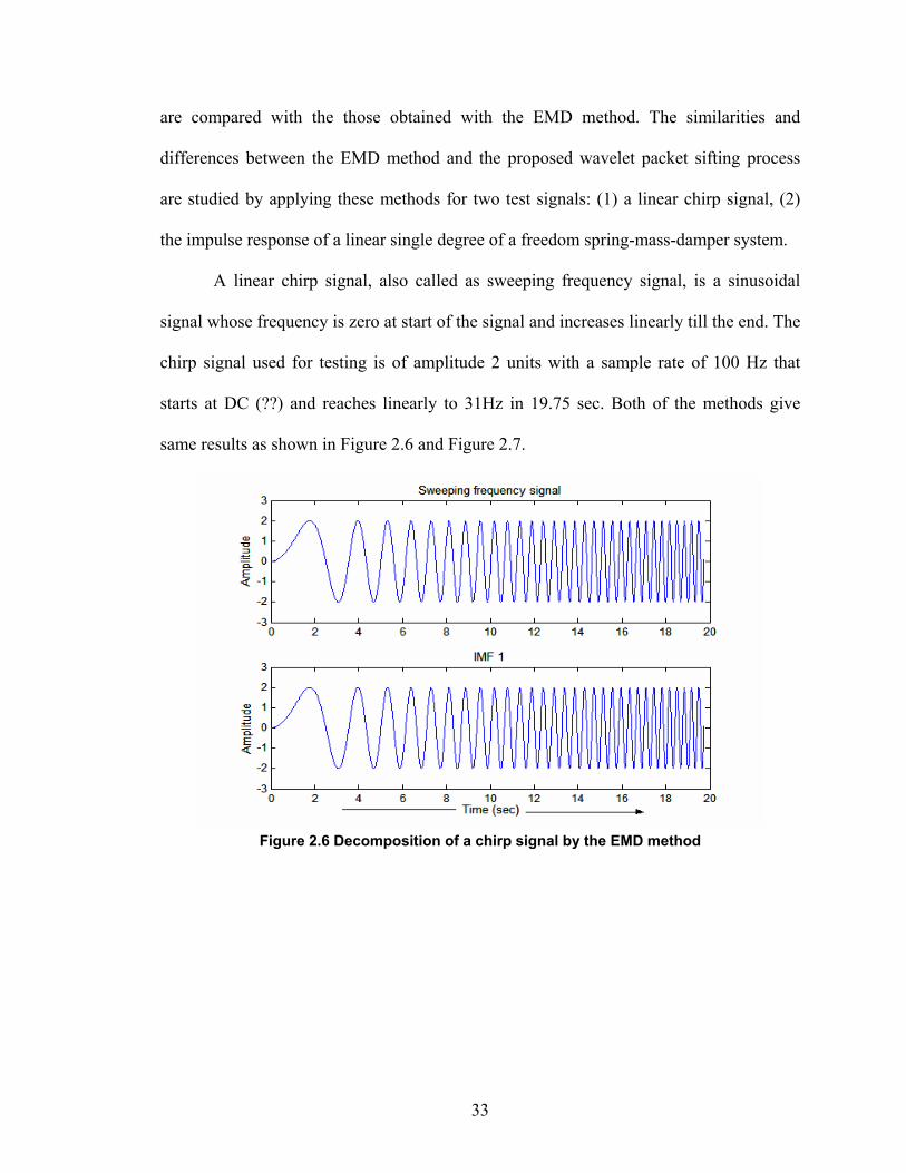
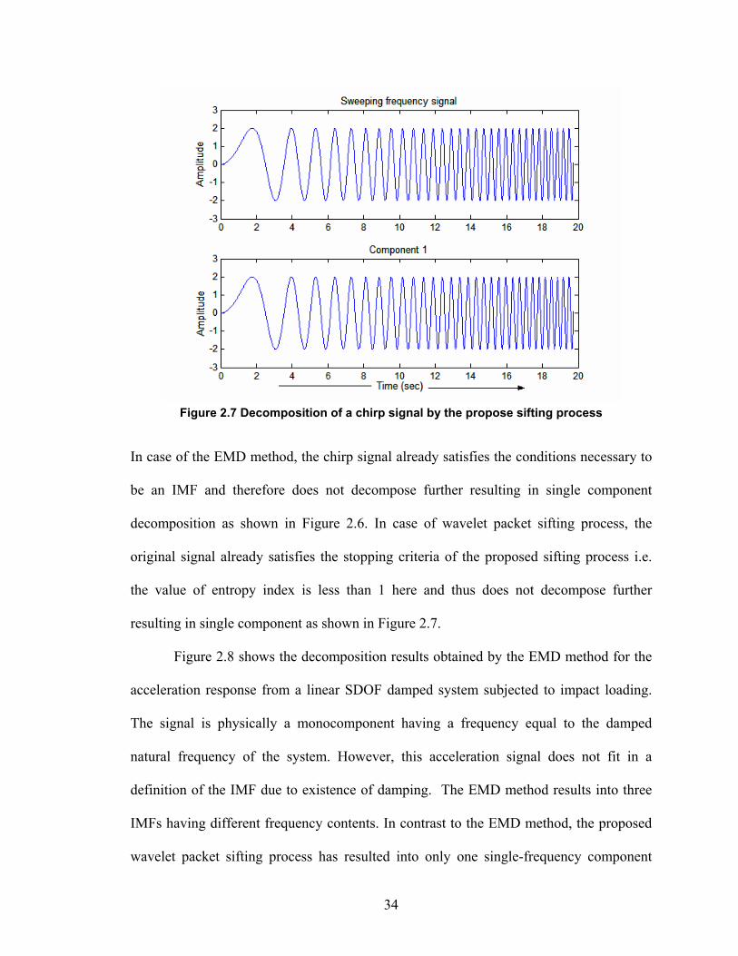
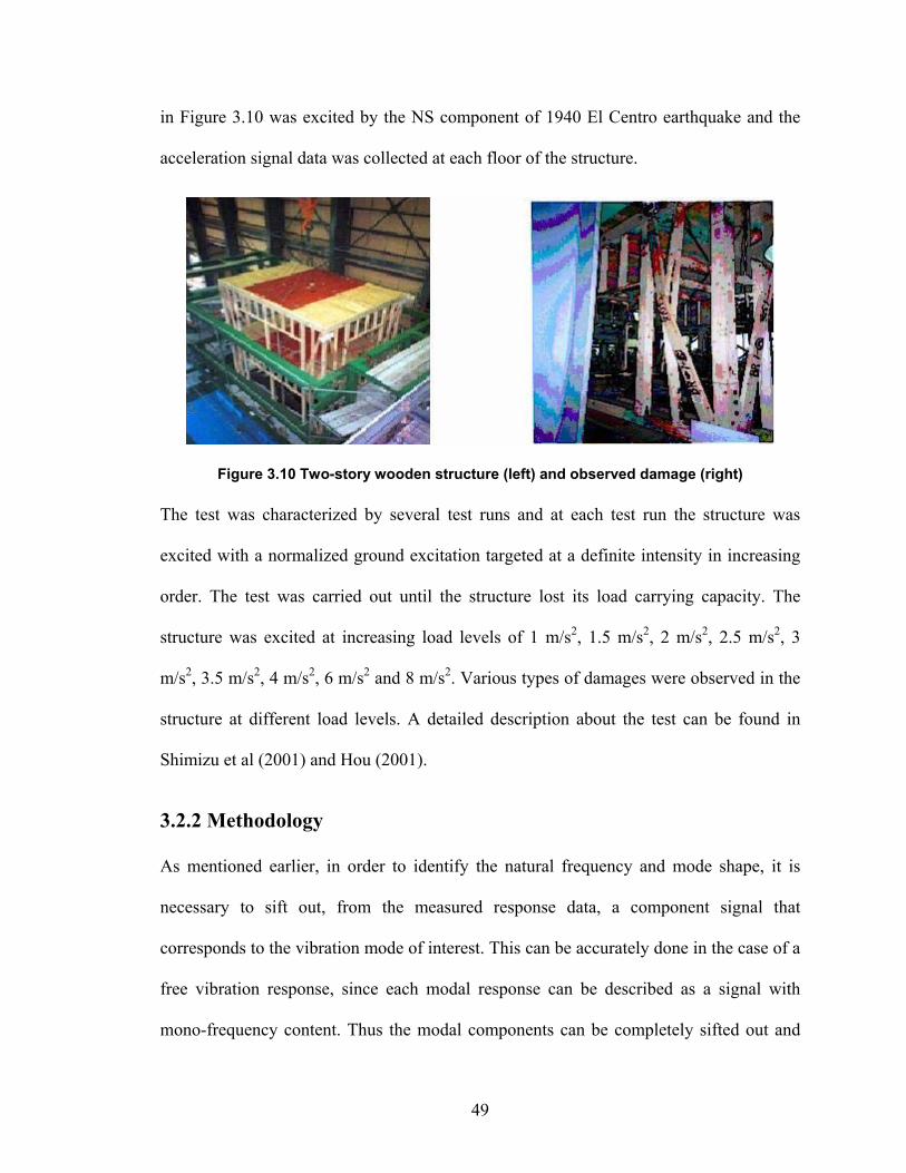
A Wavelet Packet Based Sifting Process and
Its Application for Structural Health Monitoring by
Abhijeet Dipak Shinde
A Thesis
Submitted to the Faculty of
WORCESTER POLYTECHNIC INSTITUTE
in partial fulfillment of the requirements for the
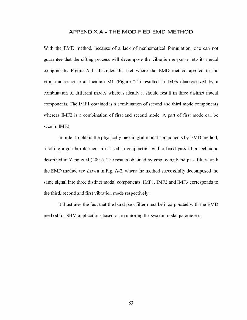
A1 Decomposition results obtained by EMD method 84
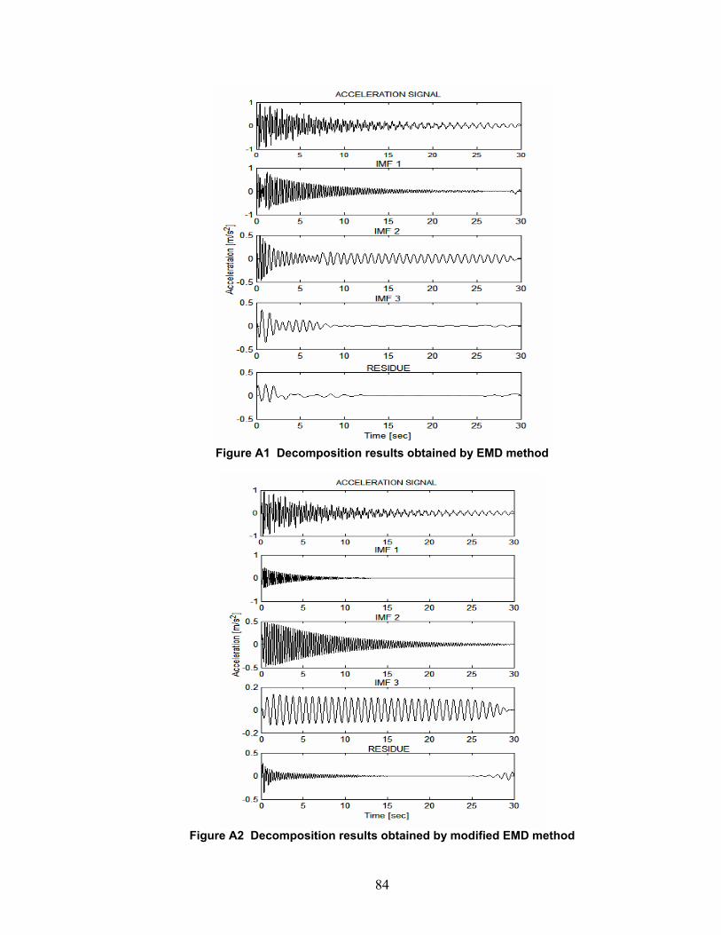
A2 Decomposition results obtained by modified EMD method 84
vii
List of Tables:
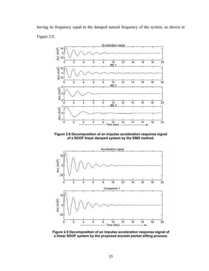
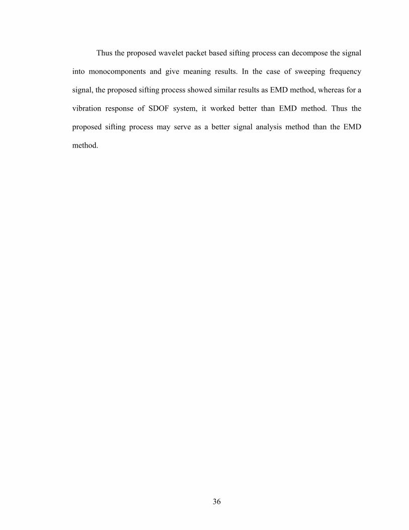
Table Page
2.1 Percentage energy contribution 29
3.1 Percentage energy contribution at various load levels 52
viii
Nomenclature: a = Dilation parameter a(t) = Instantaneous amplitude
( )iA t = Approximation component of the discrete wavelet decomposition tree at ith level b = Translation parameter
( )ic t = ith Intrinsic Mode Function (IMF) Ci = ith Damping element
( )iD t = Detail component of the discrete wavelet decomposition tree at ith level
ne = Nodal entropy in wavelet packet tree E.I. = Entropy Index
( )F t = External force matrix
( )H ω = Fourier transform of a signal Ki = ith Stiffness element Mi = ith Mass element
nr = Residue t = time
( , )fW a b = Wavelet transform of a signal
( )inormX = ith normalized mode shape vector
( )X t = Mass displacement matrix
( )X t& = Mass velocity matrix
( )X t&& = Mass acceleration matrix
z(t) = Analytic function
ix
Ø(t) = Instantaneous phase angle Ψ = Conjugate of the mother wavelet function Ψ
( )tω = Instantaneous frequency ω = Natural frequency (rad/sec)
x
1. INTRODUCTION
1.1 STRUCTURAL HEALTH MONITORING (SHM) OVERVIEW:
Structural health monitoring has become an evolving area of research in last few decades
with increasing need of online monitoring the health of large structures. The damage
detection by visual inspection of the structure can prove impractical, expensive and
ineffective in case of large structures like multistoried buildings and bridges. This
necessitates the development of structural health monitoring system that can effectively
detect the occurrence of damage in the structure and can provide information regarding
the location as well as severity of damage and possibly the remaining life of the structure.
The SHM system analyzes the structural response by excitation due to controlled or
uncontrolled loading. The controlled loading may be attributed to impulse excitation
whereas the uncontrolled loading may be attributed to the excitation by automobiles on
bridge, and a random excitation due to wind loads or an earthquake excitation.
1.1.1 Types of Damage:
Damage phenomena in a structure can be classified as linear damage and non-linear
damage. Linear damage is a case when the initially linear-elastic structure remains linear-
elastic after damage (Doebling et al, 1996). This is a case when the structure is subjected
to a sudden damage of lower intensity. The modal parameters change in this case but the
structure still exhibits linear motion after damage. This facilitates to form a simple model
of the structure and to derive equations of motion based on an assumption of linear
structural properties.
1
Non-linear damage is a case when the initially linear-elastic structure exhibits
non-linear behavior after damage. A fatigue crack initiated in shaft subjected to cyclic
loading can be called as a non-linear damage case. The crack opens and closes during
every cycle exhibiting non-linear stiffness of the shaft. Most of the damage detection
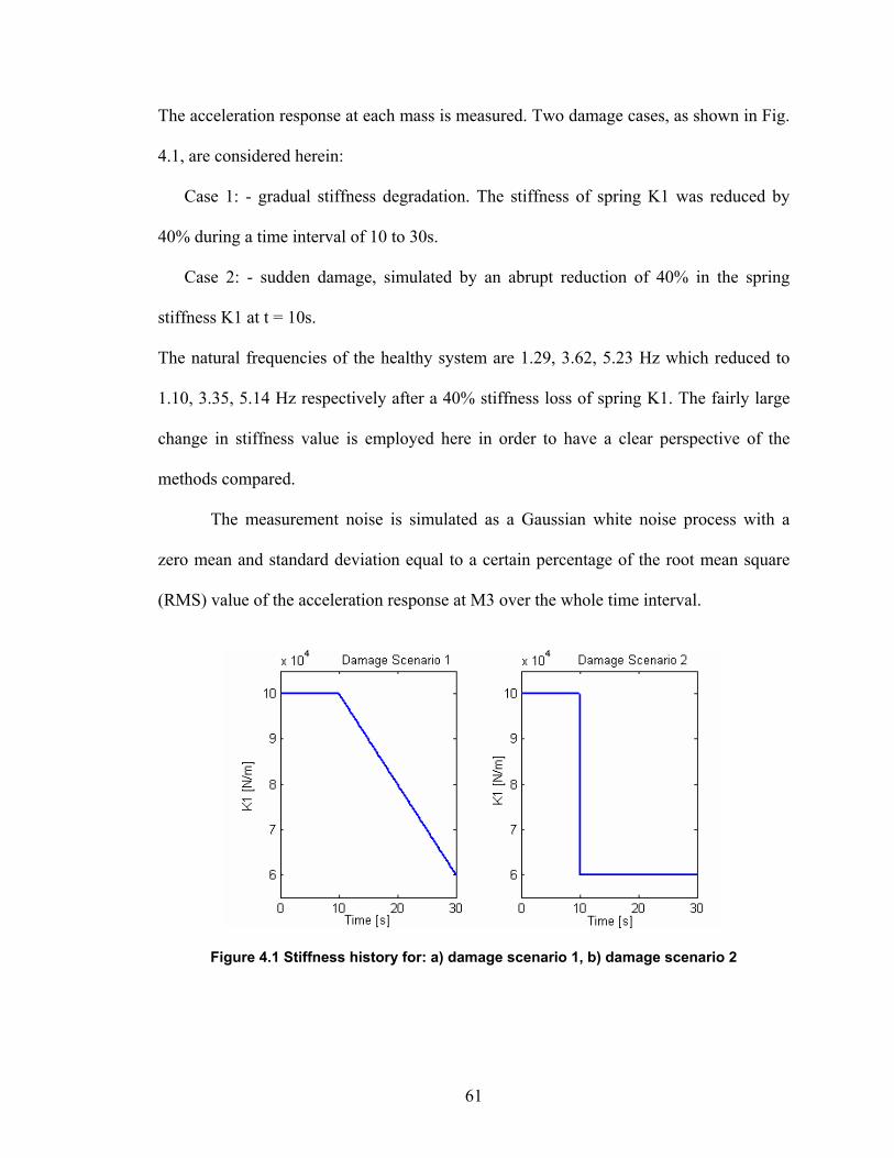
techniques assume linear damage while forming a model of the structure.
1.1.2 Types of Damage Detection Techniques:
Current damage detection methods can be mainly categorized into local damage detection
methods and global damage detection methods. In case of local damage detection
methods, the approximate location of damage in structure is known and it analyzes the
structure locally to detect the damage on or near the surface. The region of the damaged
structure needs to be easily accessible to effectively detect the exact location and severity
of damage. Some of the examples of the local damage detection techniques are eddy
current technique, acoustic or ultrasonic damage detection technique and radio graph
technique.
Contrary to the local damage detection methods, global methods do not require
prior knowledge of the location of damage in the structure to be analyzed. Global
methods monitor the changes in the vibration characteristics of the structure to detect the
location and severity of damage. The changes in dynamic properties of the structure may
be attributed to the damage occurrence in the structure as the modal parameters
comprising natural frequencies, mode shapes and damping ratio are the functions of the
physical properties(mass, damping and stiffness) of the structure. Any change in the
physical properties results change in the modal parameters.
2
1.1.3 Levels of Structural Health Monitoring:
Various global damage identification techniques have been developed till date. The
effectiveness of each method can be evaluated by the extent of the information obtained
about damage. Rytter (1993) proposed a system of classification for damage-
identification techniques which defined four levels of damage identification as follows:
Level 1: Determination that damage is present in the structure
Level 2: Determination of the geometric location of the damage
Level 3: Quantification of the severity of the damage
Level 4: Prediction of the remaining service life of the structure
Damage identification techniques used in industrial machinery may be limited to
Level 1 technique and is commonly known as fault identification technique, but most of
the damage detection techniques implemented in the SHM systems of civil infrastructures
are Level 3 or Level 4 techniques.
3
1.2 DAMAGE IDENTIFICATION TECHNIQUES:
Different types of damage identification methods based on the measurement of the
dynamic properties of the structure have been developed till date. These methods can be
categorized depending upon the type of data collected from the structure, the parameters
monitored to identify damage or technique implemented to identify damage. Some of the
methods to quote are methods monitoring changes in modal parameters, matrix update
methods, neural network based methods, pattern recognition methods, Kalman filter
based methods and methods based on statistical approach. This section summarizes all of
the above stated methods.
1.2.1 Change in Modal Parameters:
Any change in dynamic properties of structure cause change in modal properties of the
structure including change in natural frequencies, mode shapes and modal damping
values. These values can be tracked to get information about damage present in the
structure.
1.2.1.1 Change in Natural Frequency
Natural frequency of a structure is the function of stiffness and mass of the structural
members. Any damage occurred in the structure causes loss of stiffness whereas the mass
of the structural members remains the same resulting in the loss of the natural frequency
of the structure. Thus a loss in a natural frequency of the structure can be used as an
indicator of damage in the structure.
The damage identification with this technique is implemented with two types of
approaches. One of the approach models damage mathematically and predicts a natural
4
frequency of structure. The predicted natural frequency is compared it with the measured
natural frequency and damage is identified. This approach was implemented to identify a
presence of damage in the structure. Application of this approach for offshore platforms
is studied in Osegueda, et al (1992) while Silva & Gomes (1994) demonstrated use of this
approach for detecting crack length.
The second approach calculates damage parameters like crack length and location
from the frequency shifts thus measure intensity and location of damage in addition to
just damage identification as observed in the first approach. Brincker, et al. (1995a)
measured resonant frequencies and damping present in a concrete offshore oil platform
by applying auto-regressive moving average (ARMA) model to measured acceleration
response.
As a natural frequency of a structure is the global property of structure, it cannot
give spatial information about damage in the structure and thus only indicate the
occurrence of damage and only can be used as a level 1 damage detection technique.
Exception to this is a modal response at higher natural frequencies as the mode shapes are
associated with local responses at higher modal frequencies.
1.2.1.2 Change in Mode Shapes
Mode shape information can be utilized to locate damage in the structure and this
technique can be implemented as Level 3 damage detection technique. Damage present in
structure causes change in a mode shape and relative change in the mode shape can be
graphically monitored to locate damage in the structure. The mode-shapes need to be
normalized in order to effectively find the location of damage. Apart from graphical
5
monitoring of relative change in mode shape, Modal Assurance Criteria (MAC) can be
utilized to track the location of damage in the structure as described in West (1984).
1.2.2 Methods Based on Dynamic Flexibility Measurements
These methods use the dynamically measured stiffness matrix in order to detect damage.
The flexibility matrix of the structure is defined as an inverse of stiffness matrix and each
column of the flexibility matrix of the structure corresponds to the displacement pattern
of the structure when subjected to unit force at a particular node. The flexibility matrix
can be derived by calculating mass-normalized mode shapes and natural frequencies. In
case of structure having large number of degrees of freedom (DOF), due to limitations in
calculation of all mode shapes and natural frequencies, only significant low- frequency
modes and their corresponding natural frequencies are considered.
While implementing this technique, damage is detected by comparing a calculated
flexibility matrix obtained by using the modes of the damaged structure to the flexibility
matrix obtained with the modes obtained from the undamaged structure. Sometimes, for a
comparison of flexibility matrices, a flexibility matrix obtained with Finite Element
Model (FEM) of the undamaged structure may be used instead of a measured flexibility
matrix of the undamaged structure. This technique can be used as a Level 3 damage
detection technique. More information and applications of this technique can be found in
Pandey & Biswas (1994, 1995) and Salawu & Williams (1993).
1.2.3 Model Update Methods
This type of techniques uses a structural model and the structural model parameters i.e.
mass, stiffness and damping, are calculated from the equations of motion and the
6
dynamic measurements. The matrices for mass, stiffness and damping in the model are
formulated in such a way that the model response will be almost similar to the measured
dynamic response of the structure. The matrices are updated with new dynamic
measurements and the updated stiffness as well as damping matrix can be compared to
the original stiffness and damping matrix respectively to detect the location and intensity
of damage in a structure.
Various methods have been developed each with different approach for model
updating. Those can be classified in different categories depending on the objective
function for minimization problem, constraints placed on the model or numerical method
used to accomplish the optimization. For more information about model update methods,
reader is referred to Smith & Beattie (1991a) and Zimmerman & Smith (1992).
1.2.4 Neural Network (NN) based Methods
Neural Network, a concept developed as generalization of mathematical models of
human cognition or neural biology, has proven to be an efficient technique for damage
detection. According to Haykin(1998), a neural network is a massively parallel
distributed processor made of simple processing units, which has a natural propensity for
storing experimental knowledge and making it available for use. With its capacity of
performing accurate pattern recognition and classification, adaptivity, modeling non-
linearity, and learning capabilities, neural networks can be used for SHM in different
ways:
1. to model the dynamic behavior of a system or part of the system under control
(Chen et al, 1995, and Adeli, 2001)
7
2. to model the restoring forces in civil structures ( Liang et al, 1997 and Saadat,
2003)
3. to carry out pattern recognition for fault detection in rotating machinery e.g. gear
box failure (Dellomo, 1999), turbo-machinery (Kerezsi & Howard, 1995), and
bearing fault detection (Samanta et al, 2004).
Application of neural network model for SHM can also be found in Saadat (2003), where
the author used an “Intelligent Parameter Varying” (IPV) technique for health monitoring
and damage detection technique that accurately detects the existence, location, and time
of damage occurrence without any assumptions about the constitutive nature of structural
non-linearity.
The technique in Saadat(2003) was based on the concept of “gray box”, which
combined a linear time invariant dynamic model for part of the structure with a neural
network model, used to model the restoring forces in a non-linear and time-varying
system. The detailed information about the technique can be found in Nelles(2000).
Even if good results obtained with NN techniques, one of the challenges in
implementing it for a practical application in SHM is training the network. Recent work
in integration of NN with other computational techniques to enhance their performance
can be found in Adeli (2001).
1.2.5 Pattern Recognition Techniques
Damage present in the structure causes change in the modal parameters which in turn
causes change in the pattern of the structural response. This pattern can be monitored to
detect the time, location and intensity of damage. Hera & Hou (2001) successfully
detected sudden damage in ASCE benchmark structure by monitoring spikes present in
8
the higher level details of the acceleration response. A motivation behind this approach
was that a sudden damage in structure causes singularity in the acceleration response and
this singularity results in a spike in higher level details of the wavelet transform of the
signal.
Another pattern recognition method proposed by Los Alamos National
Laboratory, NM is based on statistical considerations. It proposed a statistical pattern
recognition framework which consists of the assessment of structure’s working
environment, the acquisition of structural response, the extraction of features sensitive to
damage and the development of statistical model which is used for feature discrimination.
More information and application of this method can be found in Sohn & Farrar (2001),
Sohn et al. (2001a & 2001b), Worden (2002) and Lei et al (2003).
1.2.6 Kalman Filter Technique
Kalman filter technique is the model based technique which implements an optimal
recursive data processing algorithm to estimate structural parameters necessary to
identify damage in the structure. The parameters with which damage in a structure can be
identified (stiffness and damping of the structure) can not be measured directly and in a
general practice, acceleration, velocity or displacement of the structure is measured. The
Kalman filter technique use a set of equations of motion which relate structural properties
with the measured parameters. It works in a predictor-corrector manner i.e. it estimates
the value of structural parameter based on the dynamic model and previous
measurements and then optimizes the estimated value by comparing it with the value
obtained by a measurement model and actual measurements. The optimization of the
estimated value is done to minimize the square of the difference between the estimated
9
and measured value. This technique accounts for the effect of noise introduced during
measurement as well as the effect of modeling errors. Kalman filter has been applied for
damage detection such as in Lus et al (1999).
1.2.7 Statistical Approach
This new developed technique is fundamentally based on Bayesian approach, a well
known theorem in statistical theory. An important advantage of Bayesian approach is that
it can handle the non-uniqueness of the model that can appear in the cases with
insufficient number of measurements. In order to take care of uncertainties, Beck and
Katafygiotis (1998) developed a Bayesian statistical framework for system identification
and structural health monitoring. The statistical model was developed to take care of
uncertainties introduced due to incomplete test data as a result of limited number of
sensors, noise contaminated dynamic test data, modeling errors, insensitiveness of modal
parameters to the changes in stiffness, and to describe the class of structural models
which include as much prior information as possible to reduce the uncertainties and
degree of non-uniqueness.
The method can be used for updating the system probability model to account for
above-mentioned uncertainties, and to provide a quantitative assessment of the accuracy
of results. The applications of the approach for modal identification can be found in Yuen
et al (2002), and Yuen & Katafygiotis (1998), whereas application for ASCE benchmark
SHM problem can be found in Yuen et al (2002), and Lam et al (2002).
10
1.3 SIGNAL PROCESSING METHODS
A signal collected from the accelerometers mounted on a structure can not be analyzed
directly to draw useful conclusions about damage unless the damage intensity is very
high. It needs to be processed in order to extract useful information about the structural
parameters and damage. The signal is often transformed to different domains in order to
better interpret the physical characteristics inherent in the original signal. The original
signal can be reconstructed by performing inverse operation on the transformed signal
without any loss of data. The popular methods in signal processing for SHM applications
include Fourier Analysis, Wavelet Analysis and Hilbert-Huang Analysis. All of these
methods can be distinguished from each other by a way in which it maps the signal and
have advantages over one another in terms of applicability for analyzing specific data
type. A brief introduction of each method is given below.
1.3.1 Fourier Analysis
Fourier analysis of a signal converts the signal from time domain to frequency domain.
Mathematically the Fourier transform of a signal ‘f(t)’ can be represented as
( ) ( ) tH f t e ωω∞
−
−∞
= ∫ dt (1.1)
Where ‘ ( )H ω ’ is the Fourier transform of a signal ‘f(t)’. Fourier transform represents the
signal in frequency domain and useful information about the frequency content in the
signal can be extracted. The plot of the power of Fourier transform versus frequency
exhibit peaks at the dominant frequencies present in the signal and the amplitude of the
power indicates intensity of the frequency component.
11
Note here that the Fourier transform of a signal integrates the product of the signal
with a harmonic of infinite length and the time information in the signal may be lost or
become implicit. If the signal to be analyzed is a non-stationary signal i.e. if the
amplitude or frequency is changing abruptly over time, then with the Fourier transform of
the signal , this abrupt change in time spread over the whole frequency axis in ‘ ( )H ω ’.
Thus the Fourier transform is more appropriate to analyze a stationary signal.
To cope up with a deficiency of losing time information in Fourier transform, a
Short-Time-Fourier-Transform (STFT) was developed. STFT uses a sinusoidal window
of fixed width to analyze the signal and it shifts along the data to be analyzed in order to
retain the time information in the signal. Thus in contrast to only frequency
representation ‘ ( )H ω ’ as in case of Fourier transform, STFT employs a time-frequency
representation ‘ ( ,H )ω τ ’of the signal ‘f(t’) as in the following equation 1.2.
*( , ) ( ) ( ) tH f t g t e ωω τ τ −= − dt∫ (1.2)
where g(t-τ) is a window function. Once the window width is chosen, then the time-
frequency resolution obtained remains fixed over entire time-frequency plane and one
can either get good time resolution or good frequency resolution in the analysis but not
both. More information about the STFT can be found in Allen & Rabiner (1977) and
Rioul & Vetterli (1991).
Because of its ability to identify the frequency content and intensity of the
frequency component of a signal, significant information about the modal parameters i.e.
natural frequency, mode shapes and damping can be extracted from the Fourier transform
of the structural response. Various methods of fault diagnosis and damage detection
12
based on the Fourier transform of the vibration response of the structure can be found in
Chiang et al (2001).
1.3.2 Wavelet Analysis
Analyzing the response data of general transient nature without knowing when the
damage occurred, inaccurate results may be presented by the traditional Fourier analysis
due to its time integration over the whole time span. Moreover, damage could develop in
progressively such as stiffness degradation due to mechanical fatigue and chemical
corrosion and a change in stiffness might never been found. As an extension of the
traditional Fourier analysis, wavelet analysis provides a multi-resolution and time-
frequency analysis for non-stationary data and therefore can be effectively applied for
structural health monitoring.
1.3.2.1 Continuous Wavelet Transform (CWT)
The Continuous Wavelet Transform (CWT) of a signal f(t), Wf(a,b) , is defined as
W a ba
f t t ba
dtf ( , ) ( ) * ( )=−
−∞
∞
∫1
Ψ (1.3)
Here ‘Ψ ’ is the conjugate of a mother wavelet function ‘Ψ ’, ‘a’ and ‘b’ are called as
the dilation parameter and the translation parameter, respectively. Both of the
parameters are real and ‘a’ must be positive. The mother wavelet ‘ ’ needs to satisfy
certain admissibility condition in order to ensure existence of the inverse wavelet
transform.
Ψ
The dilation parameter ‘a’ and the translation parameter ‘b’ are also referred as
the scaling and shifting parameters respectively and play an important role in the wavelet
analysis. By varying the value of translation parameter ‘b’, a signal is examined by the
13
wavelet window piece by piece localized in the neighborhood of ‘t=b’ and so the non-
stationary nature of the data can be examined which is similar to the Short Time Fourier
Transform (STFT). By varying the value of dilation parameter ‘a’, the data portion in the
neighborhood of ‘b’ can be examined in different resolutions and so a time varying
frequency content of the signal can be revealed by this multi-resolution analysis, a feature
the STFT doesn’t have. The continuous wavelet transform maps the signal on a Time-
Scale plane. The concept of scale in Wavelet analysis is similar to the concept of
frequency in Time-Frequency analysis. The scale is inversely proportional to the
frequency. Performing the inverse wavelet transform on the wavelet transform of a
signal, the original signal can be reconstructed without any loss of data. For detailed
information of wavelet transform, readers are referred to Rioul & Vetterli (1991) and
Daubechies (1992). Early applications of wavelets for damage detection of mechanical
systems were summarized in Staszewski (1998).
1.3.2.2 Discrete Wavelet Transform (DWT)
The computational cost of performing continuous wavelet transform is reduced by
implementing Discrete Wavelet Transform (DWT). In DWT the dilation parameter ‘a’
and the translation parameter ‘b’ are discretized by using the dyadic scale i.e.
a = 2j b = k.2j j k z, ∈ (1.4)
Here z is the set of positive integers.
In the case of DWT, the wavelet plays a role of dyadic filter. The DWT analyzes
the signal by implementing a wavelet filter of particular frequency band to shift along a
time axis. The frequency band of the filter depends on the level of decomposition and by
shifting it in the time domain, the local examination of the signal becomes possible. As a
14
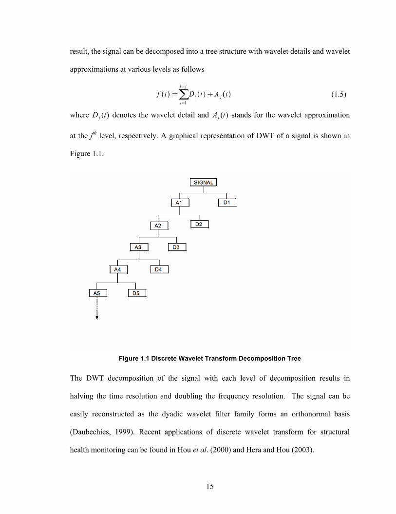
result, the signal can be decomposed into a tree structure with wavelet details and wavelet
approximations at various levels as follows
f t D t A ti ji
i j
( ) ( ) )= +=
=
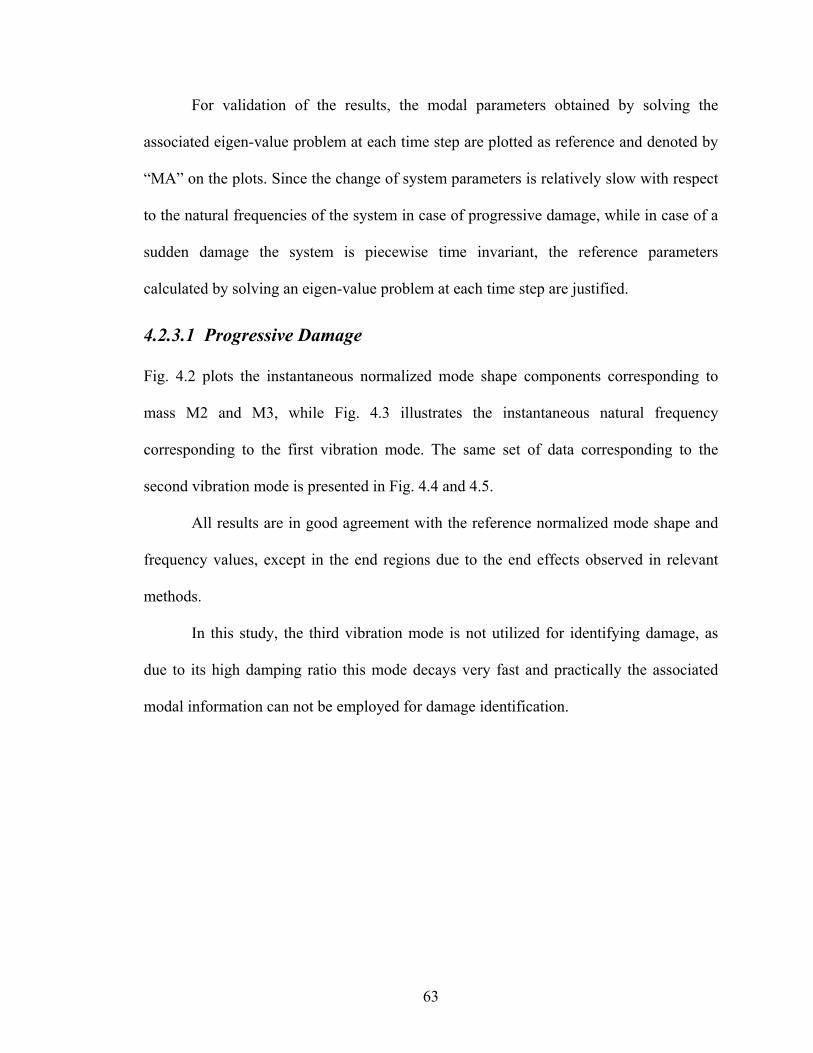
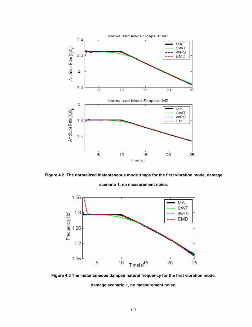
∑1
(
(1.5)
where denotes the wavelet detail and stands for the wavelet approximation
at the jth level, respectively. A graphical representation of DWT of a signal is shown in
Figure 1.1.
)(tD j )(tAj
Figure 1.1 Discrete Wavelet Transform Decomposition Tree
The DWT decomposition of the signal with each level of decomposition results in
halving the time resolution and doubling the frequency resolution. The signal can be
easily reconstructed as the dyadic wavelet filter family forms an orthonormal basis
(Daubechies, 1999). Recent applications of discrete wavelet transform for structural
health monitoring can be found in Hou et al. (2000) and Hera and Hou (2003).
15
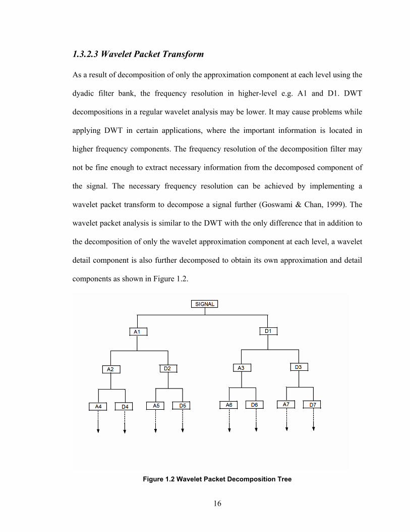
1.3.2.3 Wavelet Packet Transform
As a result of decomposition of only the approximation component at each level using the
dyadic filter bank, the frequency resolution in higher-level e.g. A1 and D1. DWT
decompositions in a regular wavelet analysis may be lower. It may cause problems while
applying DWT in certain applications, where the important information is located in
higher frequency components. The frequency resolution of the decomposition filter may
not be fine enough to extract necessary information from the decomposed component of
the signal. The necessary frequency resolution can be achieved by implementing a
wavelet packet transform to decompose a signal further (Goswami & Chan, 1999). The
wavelet packet analysis is similar to the DWT with the only difference that in addition to
the decomposition of only the wavelet approximation component at each level, a wavelet
detail component is also further decomposed to obtain its own approximation and detail
components as shown in Figure 1.2.
Figure 1.2 Wavelet Packet Decomposition Tree
16
Each component in this wavelet packet tree can be viewed as a filtered component with a
bandwidth of a filter decreasing with increasing level of decomposition and the whole
tree can be viewed as a filter bank. At the top of the tree, the time resolution of the WP
components is good but at an expense of poor frequency resolution whereas at the bottom
of the tree, the frequency resolution is good but at an expense of poor time resolution.
Thus with the use of wavelet packet analysis, the frequency resolution of the decomposed
component with high frequency content can be increased. As a result, the wavelet packet
analysis provides better control of frequency resolution for the decomposition of the
signal.
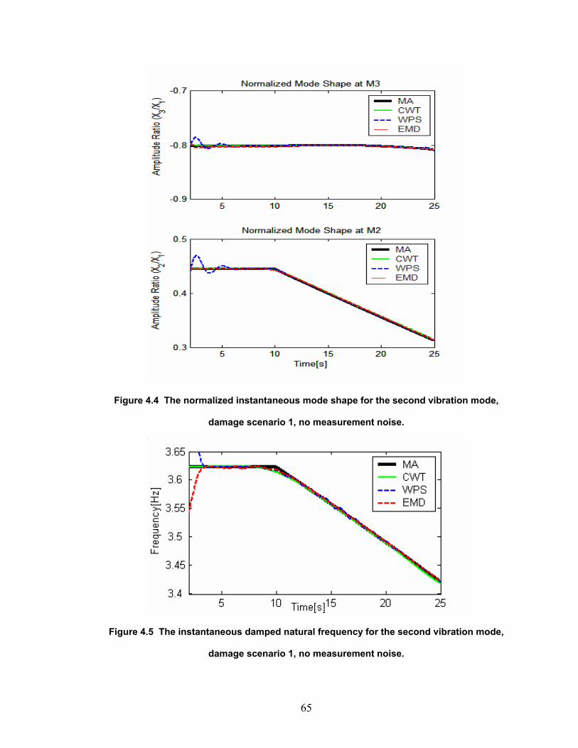
1.3.3 Hilbert-Huang Analysis
NASA Goddard Space Flight Center (GSFC) has developed a signal analysis method,
called as the Empirical Mode Decomposition (EMD) method, which analyzes the signal
by decomposing the signal into its monocomponents, called as Intrinsic Mode Functions
(IMF) (Huang et al, 1998). The empirical nature of the approach may be partially
attributed to a subjective definition of the envelope and the intrinsic mode function
involved in its sifting process. The EMD method used in conjunction with Hilbert
Transform is also known as ‘Hilbert-Huang Transform’ (HHT). Because of its
effectiveness in analyzing a nonlinear, non-stationary signal, the HHT was recognized as
one of the most important discoveries in the field of applied mathematics in NASA
history. By the EMD method, discussed in more details later in ‘Section 1.4’, the original
signal ‘f(t)’ can be represented in terms of IMFs as:
f t c t ri ni
n
( ) ( )= +=∑
1 (1.6)
17
where C i (t) is the ith Intrinsic Mode Function and rn is the residue.
A set of analytic functions can be constructed for these IMFs. The analytic
function ‘z(t)’ of a typical IMF ‘c(t)’ is a complex signal having the original signal ‘c(t)’
as the real part and its Hilbert transform of the signal as its imaginary part. By
representing the signal in the polar coordinate form one has
[ ] ( )( ) ( ) ( ) ( ). j tz t c t jH c t a t e φ= + = (1.7)
where ‘a(t)’ is the instantaneous amplitude and ‘Ø(t)’ is the instantaneous phase
function. The instantaneous amplitude ‘a(t)’ and is the instantaneous phase function
‘Ø(t)’ can be calculated as
{ } { }2 2( ) ( ) [ ( )]a t c t H c t= + (1.8)
1 [ ( )]( ) tan( )
H c ttc t
φ − =
(1.9)
The instantaneous frequency of a signal at time t can be expressed as the rate of change
of phase angle function of the analytic function obtained by Hilbert Transform of the
signal (Ville, 1948). The expression for instantaneous frequency is given in equation 1.10
( )( ) d ttdtφω = (1.10)
Because of a capability of extracting instantaneous amplitude ‘a(t)’ and instantaneous
frequency ‘ ( )tω ’ from the signal, this method can be used to analyze a non-stationary
vibration signal. In a special case of a single harmonic signal, the phase angle of its
Hilbert transform is a linear function of time and therefore its instantaneous frequency is
constant and is exactly equal to the frequency of the harmonic. In general, the concept of
instantaneous frequency provides an insightful description as how the frequency content
of the signal varies with the time. The method can be used for damage detection and
18
system identification and the relevant applications can be found in Vincent et al (1999),
Yang & Lei (2000), Yang et al (2003a, 2003b, 2004).
19
1.4 MOTIVATION
The Empirical Mode Decomposition (EMD) method proposed by Huang et al (1998)
decomposes a signal into IMFs by an innovative sifting process. The IMF is defined as a
function which satisfy following two criterion
(i) The number of extrema and the number of zero crossings in the component
must either equal or differ at most by one
(ii) At any point, the mean value of the envelope defined by the local maxima and
the envelope defined by local minima is zero.
A sifting process proposed to extract IMFs from the signal process the signal iteratively
in order to obtain a component which satisfies above mentioned conditions. An intention
behind application of these constraints on the decomposed components was to obtain a
symmetrical mono-frequency component to guarantee a well-behaved Hilbert transform.
It is shown that the Hilbert transform behaves erratically if the original function is not
symmetric with X-axis or there is sudden change in phase of the signal without crossing
X-axis (Huang et al, 1998).
Although the IMFs are well behaved in their Hilbert Transform, it may not
necessarily have any physical significance. For example, an impulse response of a simple
linear damped oscillator, which is physically mono-component with a single frequency,
may not be necessarily fit the definition of the IMF and envelope function as illustrated in
the comparison study shown in Section 2.4. Moreover the empirical sifting process does
not guarantee exact modal decomposition. The EMD method proposed in Huang et al
(1996) may lead to mode mixture and the analyzing signal needs to pass through a
bandpass filter before analysis by EMD method (Appendix A).
20
The sifting process separates the IMFs with decreasing order of frequency i.e it
separates high frequency component first and decomposes the residue obtained after
separating each IMF till a residue of nearly zero frequency content does not obtained. Till
date, there is no mathematical formulation derived for EMD method and the studies done
in order to analyze the behavior of this method in stochastic situations involving
broadband noise shows that the method behaves a dyadic filter bank when applied to
analyze a fractional Gaussian noise (Flandrin et al, 2003). In this sense, the sifting
process in the EMD method may be viewed as an implicit wavelet analysis and the
concept of the intrinsic mode function in the EMD method is parallel to the wavelet
details in wavelet analysis.
The wavelet packet analysis of the signal also can be seen as a filter bank with
adjustable time and frequency resolution. It results in symmetrical orthonormal
components when a symmetrical orthogonal wavelet is used as a decomposition wavelet.
As a signal can be decomposed into symmetrical orthonormal components with wavelet
packet decomposition, they also guarantee well behaved Hilbert transform. These facts
motivated to formulate a sifting process based on wavelet packet decomposition to
analyze a non-stationary signal, and it may be used as a damage detection technique for
structural health monitoring.
21
2. A WAVELET PACKET BASED SIFTING PROCESS
2.1 MATHEMATICAL BACKGROUND
This section briefly describes the mathematical theory behind the terminology used in the
development of wavelet packet based sifting process.
2.1.1 Wavelet Packet Transform A wavelet packet is represented as a function, ,
ij kψ , where ‘i’ is the modulation parameter,
‘j’ is the dilation parameter and ‘k’ is the translation parameter.
/ 2, ( ) 2 (2 )i j i j
j k t t kψ ψ− −= − (2.1)
Here i = 1,2…jn and ‘n’ is the level of decomposition in wavelet packet tree. The wavelet
iψ is obtained by the following recursive relationships:
2 1( ) ( ) ( )22
i i
k
tt h k kψ ψ∞
=−∞
= −∑
(2.2)
2 1 1( ) ( ) ( )22
i i
k
tt g k kψ ψ∞
+
=−∞
= −∑ (2.3)
Here is called as a mother wavelet and the discrete filters h k and 1( )tψ ( ) ( )g k are
quadrature mirror filters associated with the scaling function and the mother wavelet
function (Daubechies, 1992).
The wavelet packet coefficients ,ij kc corresponding to the signal f(t) can be obtained as,
, ,( ) ( )i ij k j kc f t tψ
∞
−∞
= ∫ dt (2.4)
provided the wavelet coefficients satisfy the orthogonality condition.
The wavelet packet component of the signal at a particular node can be obtained as
22
, ,( ) ( )i i ij j k j k
kf t c tψ
∞
=−∞
= ∑ dt (2.5)
After performing a wavelet packet decomposition up to jth level, the original signal can be
represented as a summation of all wavelet packet components at jth level as shown in
Equation 2.6
2
1( ) ( )
j
ij
if t f
=
=∑ t (2.6)
2.1.2 Wavelet Packet Node Entropy and Entropy Index
The entropy ‘E’ is an additive cost function such that E(0)=0. The entropy indicates the
amount of information stored in the signal i.e. higher the entropy, more is the information
stored in the signal and vice-versa. There are various definitions of entropy in the
literature (Coifman and Wickerhauser, 1992). Among them, two representative ones are
used here i.e. the energy entropy and the Shannon entropy. The wavelet packet node
energy entropy at a particular node ‘n’ in the wavelet packet tree of a signal is a special
case of P=2 of the P-norm entropy which is defined as
, ( 1Pi
n j kk
e c P )= ≥∑ (2.7)
where ,ij kc are the wavelet packet coefficients at particular node of wavelet packet tree. It
was demonstrated that the wavelet packet node energy has more potential for use in
signal classification as compared to the wavelet packet node coefficients alone (Yen and
Lin 2000). The wavelet packet node energy represents energy stored in a particular
frequency band and is mainly used to extract the dominant frequency components of the
signal. The Shannon entropy is defined as
23
2 2, ,( ) log ( )i i
n j k jk
e c c k = − ∑ (2.8)
Note that one can define his/her own entropy function if necessary. Here the entropy
index (EI) is defined as a difference between the number of zero crossings and the
number of extrema in a component corresponding to a particular node of the wavelet
packet tree as
. . _ _ _ _ _E I No of zero cross No of extrema= − (2.9)
Entropy index value greater than 1 indicates that the component has a potential to reveal
more information about the signal and it needs to be decomposed further in order to
obtain simple frequency components of the signal.
2.2 METHODOLOGY The proposed wavelet based sifting process starts with interpolation of data with cubic
spline interpolation. The interpolated data increases the time resolution of the signal
which will in turn increase the regularity of the decomposed components. The cubic
spline interpolation assures the conservation of signal data between sampled points
without large oscillations.
The interpolated data is decomposed into different frequency components by
using wavelet packet decomposition. A shape of the decomposed components by wavelet
analysis depends on the shape of the mother wavelet used for decomposition. A
symmetrical wavelet is preferred as a mother wavelet in the process to guarantee
symmetrical and regular shaped decomposed components. Daubechies wavelet of higher
order and discretized Meyer wavelet shows good symmetry and leads to symmetrical and
regular shaped components.
24
In case of the binary wavelet packet tree, decomposition at level ‘n’ results in 2n
components. This number may become very large at a higher decomposition level and
necessitate increased computational efforts. An optimum decomposition of the signal can
be obtained based on the conditions required to be an IMF. A particular node (N) is split
into two nodes N1 and N2 if and only if the entropy index of the corresponding node is
greater than 1 and thus the entropy of the wavelet packet decomposition is kept as least as
possible. Other criteria such as the minimum number of zero crossings and the minimum
peak value of components can also be applied to decompose only the potential
components in the signal.
Once the decomposition is carried out, the mono-frequency components of the
signal can be sifted out from the components corresponding to the terminal nodes of the
wavelet packet tree. The percentage energy contribution of the component corresponding
to each terminal node to the original signal is used as sifting criteria in order to identify
the potential components of the signal. This is obtained by summing up the energy
entropy corresponding to the terminal nodes of the wavelet packet tree of the signal
decomposition in order to get total energy content and then calculating the percentage
contribution of energy corresponding to each terminal node to the total energy. Higher
the percentage energy contribution, more significant is the component. Note that the
decomposition is unique if the mother wavelet in the wavelet packet analysis is given and
the sifting criteria are specified.
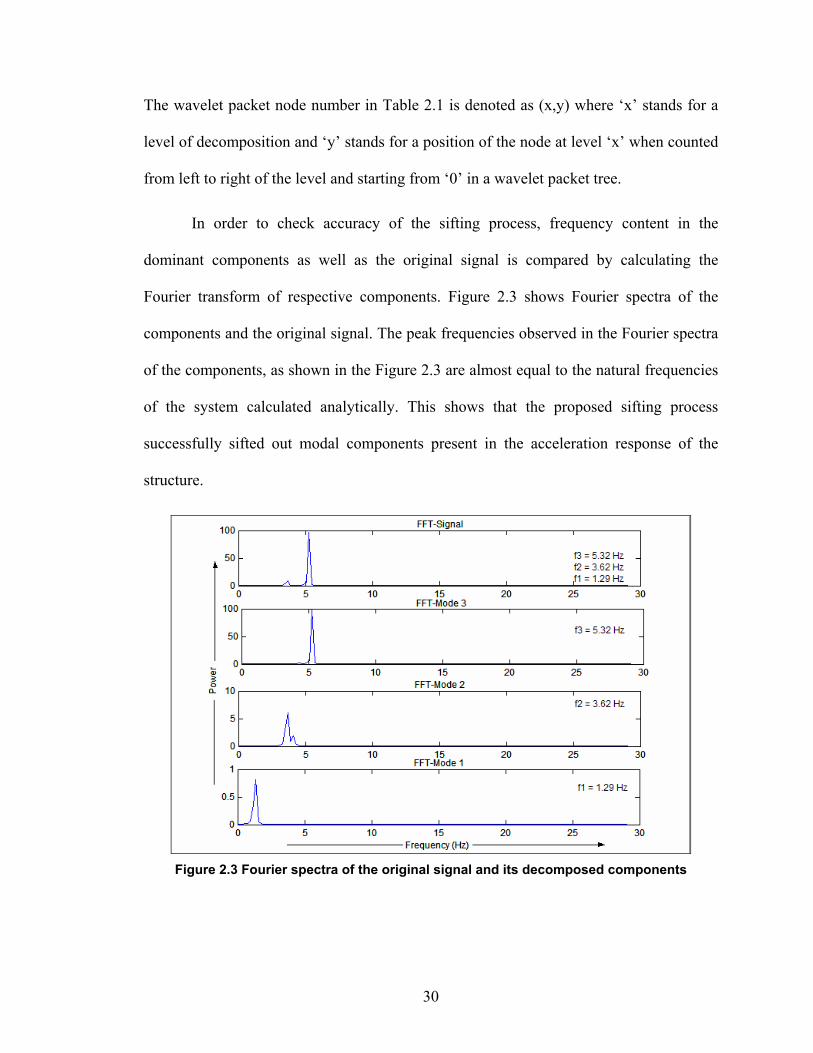
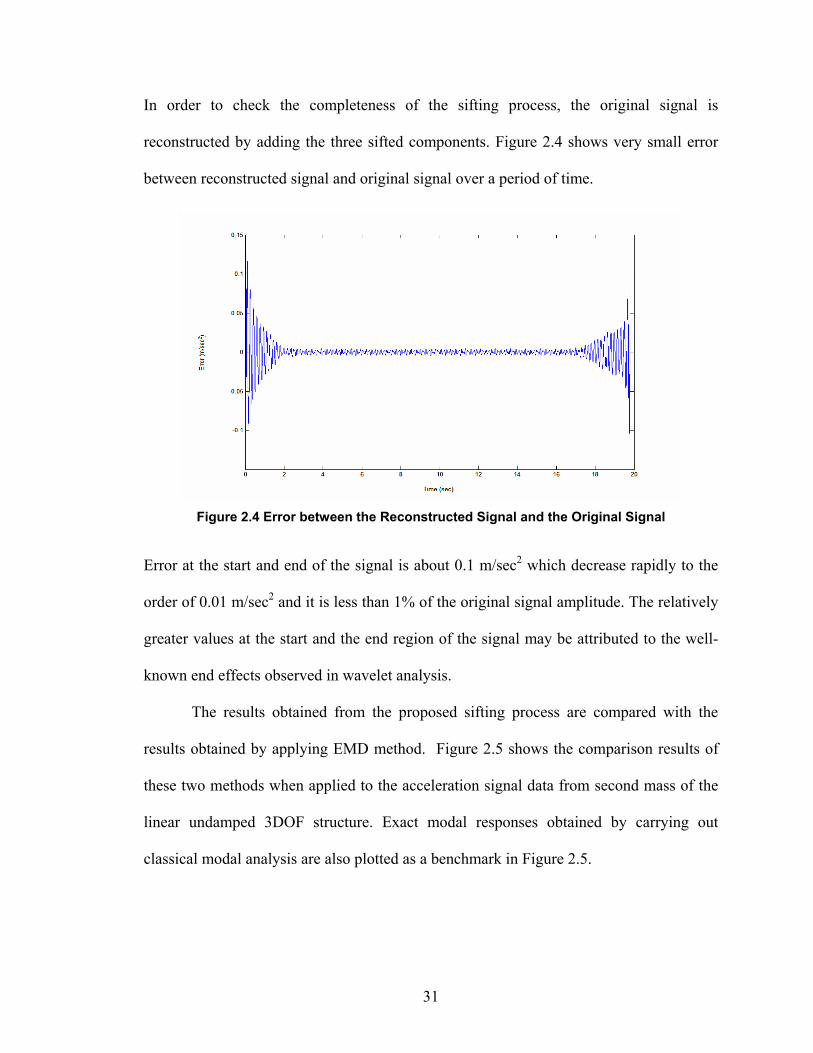
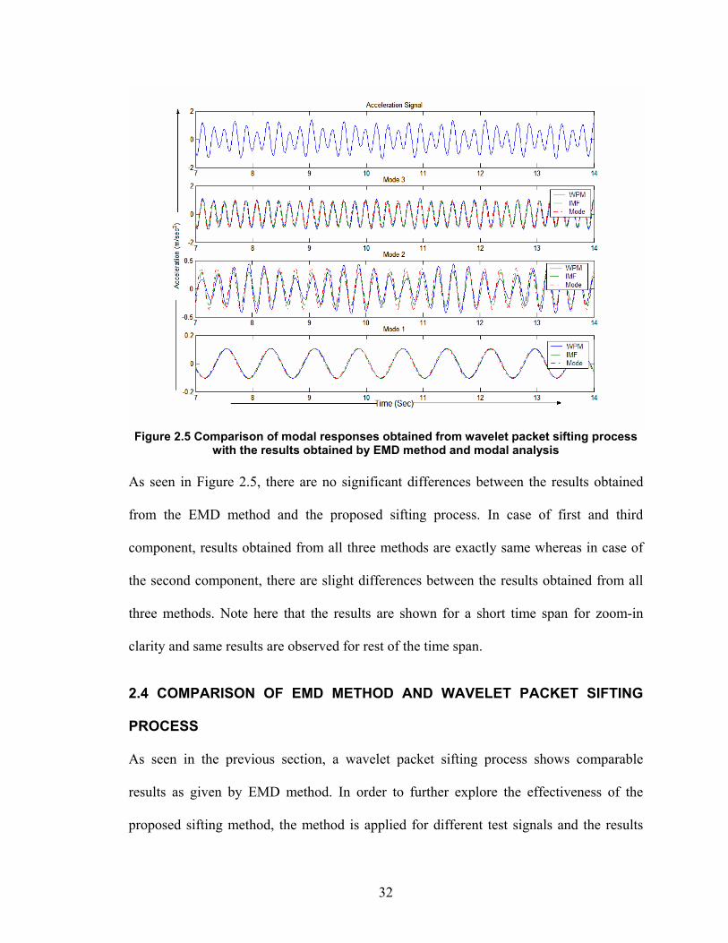
2.3 VALIDATION OF THE WAVELET PACKET BASED SIFTING PROCESS
This section validates the proposed wavelet packet based sifting process by analyzing an
acceleration response of a three storied structure. A simulation model consisting a linear
25
3 degree of freedom (DOF) spring-mass-damper system has been used for this purpose
and the results have been compared to the analytical results as well as to the results
obtained by Empirical Mode Decomposition method.
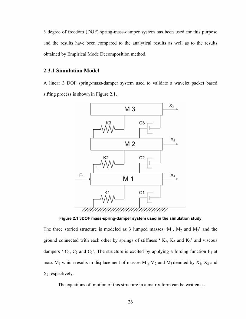
2.3.1 Simulation Model
A linear 3 DOF spring-mass-damper system used to validate a wavelet packet based
sifting process is shown in Figure 2.1.
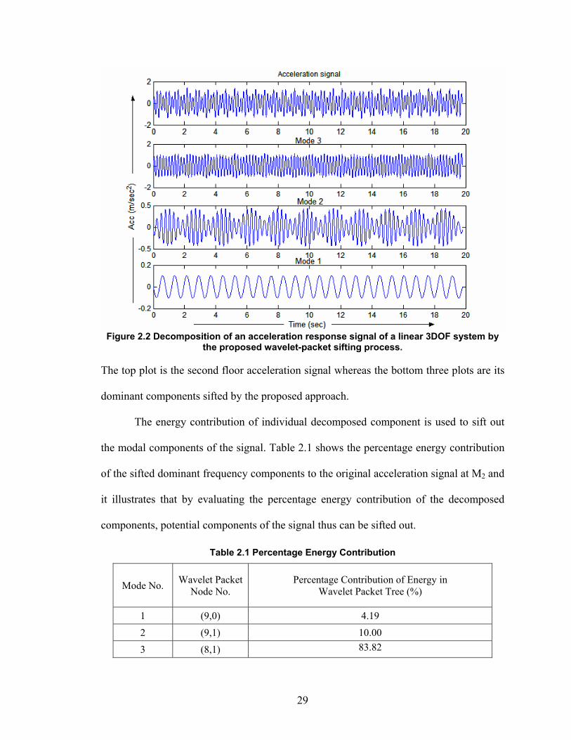
Figure 2.1 3DOF mass-spring-damper system used in the simulation study The three storied structure is modeled as 3 lumped masses ‘M1, M2 and M3’ and the
ground connected with each other by springs of stiffness ‘ K1, K2 and K3’ and viscous
dampers ‘ C1, C2 and C3’. The structure is excited by applying a forcing function F1 at
mass M1 which results in displacement of masses M1, M2 and M3 denoted by X1, X2 and
X3 respectively.
The equations of motion of this structure in a matrix form can be written as
26
( ) ( ) ( ) ( )MX t CX t KX t F t+ + =&& & (2.10)
Here M, C and K are mass, damping and stiffness matrices of the structure, respectively
where
1 1 2 2 1 1
2 2 2 3 3 2 2
3 3 3
0 0 0 00 0 , ,0 0 0 0
M K K K C C C2
3 3
3 3
M M K K K K K C C C C CM K K C C
+ − + − = = − + − = − + − −
−
A subscript indicates mass number. In Equation 2.10, F(t) is a force function matrix
whereas X(t), ( )X t& and ( )X t&& are displacement, velocity and acceleration response


![1935. Fault diagnosis of gearboxes using wavelet support ... · Zeng [30] developed an intelligent fault diagnosis procedure based on wavelet packet transform (WPT) and hybrid SVM.](https://static.documents.pub/doc/80x56/5ffde5fc9f248533cc39c91d/1935-fault-diagnosis-of-gearboxes-using-wavelet-support-zeng-30-developed.jpg)

