ECCOMAS Congress 2016 VII European Congress on Computational Methods in Applied Sciences and Engineering M. Papadrakakis, V. Papadopoulos, G. Stefanou, V. Plevris (eds.) Crete Island, Greece, 5–10 June 2016 A WAY TO IMPROVE JET MODELING WITHIN RANS EQUATION SYSTEM Alexey Troshin 1,2 1 Central Aerohydrodynamic Institute (TsAGI) 1 Zhukovsky Street, Zhukovsky, Moscow Region, 140180, Russia 2 Moscow Institute of Physics and Technology (MIPT) 9 Institutskiy per., Dolgoprudny, Moscow Region, 141700, Russia e-mail: [email protected]Keywords: Turbulence Model, Mixing Layer, Jet. Abstract. Performance of several standard turbulence models in predicting the flow field of a plane jet is analyzed. Jet potential core length is shown to be overestimated by all the models considered. To solve the problem, an additional source term in the turbulence characteristic frequency ω equation is used. It accounts the longitudinal flow inhomogeneity and entrainment which influence turbulence in jet mixing layers. In comparison to the earlier publications on this source term, a coefficient in its formulation has been slightly altered to better predict round jets. The modified SSG/LRR-ω differential Reynolds stress model is used to compute several test cases including free subsonic plane and round jets, a supersonic underexpanded free round jet, and a coaxial jet. In all the cases, improvements over the standard SSG/LRR-ω and SST models are shown. Further steps involving RANS turbulence models verification with high order of accuracy LES computations are discussed. 1
Transcript
ECCOMAS Congress 2016VII European Congress on Computational Methods in Applied Sciences and Engineering
M. Papadrakakis, V. Papadopoulos, G. Stefanou, V. Plevris (eds.)Crete Island, Greece, 5–10 June 2016
A WAY TO IMPROVE JET MODELING WITHIN RANS EQUATIONSYSTEM
Alexey Troshin1,2
1Central Aerohydrodynamic Institute (TsAGI)1 Zhukovsky Street, Zhukovsky, Moscow Region, 140180, Russia
2Moscow Institute of Physics and Technology (MIPT)9 Institutskiy per., Dolgoprudny, Moscow Region, 141700, Russia
Abstract. Performance of several standard turbulence models in predicting the flow field of aplane jet is analyzed. Jet potential core length is shown to be overestimated by all the modelsconsidered. To solve the problem, an additional source term in the turbulence characteristicfrequency ω equation is used. It accounts the longitudinal flow inhomogeneity and entrainmentwhich influence turbulence in jet mixing layers. In comparison to the earlier publications onthis source term, a coefficient in its formulation has been slightly altered to better predict roundjets. The modified SSG/LRR-ω differential Reynolds stress model is used to compute several testcases including free subsonic plane and round jets, a supersonic underexpanded free round jet,and a coaxial jet. In all the cases, improvements over the standard SSG/LRR-ω and SST modelsare shown. Further steps involving RANS turbulence models verification with high order ofaccuracy LES computations are discussed.
1
Alexey Troshin
1 INTRODUCTION
Today it is widely recognized that most turbulence models overestimate jet potential corelength Lini. In [1] Lini overprediction is reported for k − ε and SST models, in [2] the same isshown for an EARSM, and in [3] SSG/LRR-ω differential Reynolds stress model (DRSM) isfound to give similar results. This issue can negatively influence the modeling of many problemsinvolving civil aircraft propulsive jets, their interaction with nozzle walls and downstream struc-tural elements of a plane. Several solutions of this problem have been proposed. In [1], Lini isreduced by taking into account the increase in turbulent diffusion intensity near the jet axis dueto acoustic interaction between different parts of the mixing layer; in [4], another modificationof turbulent diffusion is proposed compatible with the concept of mixing layer self-similarity.In [3], the problem is further investigated and another approach to improve the jet potential coremodeling is developed which is not connected to the amplification of the modeled turbulencediffusion. Instead, the influence of longitudinal mean flow inghomogeneity on turbulence statis-tics is analyzed and taken into account. This approach is followed in the present paper. Firstly,more computational results confirming the inadequacies of standard models in predicting Lini
are presented. After that, a minor update to one of the coefficients in the model proposed in[3] is made. Finally, new test cases computations using both modified and original models arereported.
The structure of the paper is as follows. In Section 2, the results of free plane jet compu-tations using several standard turbulence models are compared, and common shortcomings ofthe solutions are discussed. In Section 3, a modification to the SSG/LRR-ω turbulence model isformulated and briefly commented. In Section 4, the computations of free subsonic plane andround jets, a supersonic underexpanded free round jet, and a coaxial jet are reported, and per-formance of the modified model is compared to the standard one and to the eddy viscosity SSTmodel. Further steps in RANS turbulence models verification involving high order of accuracyLES computations are discussed in Section 5. The conclusions are made in Section 6.
2 STANDARD TURBULENCE MODELS
2.1 Solver and turbulence models
All the computations presented here are conducted using the EWT-TsAGI in-house code[5]. The solver uses structured multiblock hexahedral meshes. Hanging nodes at the blockboundaries are allowed.
The following complete unsteady equation systems for the compressible air flow can besolved by the code:
• Euler equations;
• Navier–Stokes equations;
• Favre averaged Reynolds equations with one of the turbulence models listed below:
— Menter SST model [6];
— Coakley q − ω model [7];
— Spalart–Allmaras model [8];
— Wilcox Stress-ω DRSM [9];
— SSG/LRR-ω DRSM [10] and its modified version [3].
2
Alexey Troshin
Second order of accuracy finite volume Godunov–Kolgan–Rodionov scheme is implementedin the solver. Explicit second order two step time marching (global, fractional, and local timesteppings), first order backward Euler unconditionally stable implicit time marching (global andlocal time steppings), and second order dual time stepping are available.
The following notes concerning the numerical method need to be made. First, turbulencevariables at a face of a cell are reconstructed with the same method (using van Leer limiterby default) as main variables thus maintaining the same accuracy order for all the equations.Second, exact iterative Godunov Riemann solver is used (turbulence variables are treated aspassive scalars). To our experience, these features, aimed at increasing the accuracy of themethod, generally do not degrade convergence.
Since the test cases reported here are steady, implicit scheme has been used in the computa-tions.
2.2 Test case specification
To demonstrate the performance of the standard turbulence models, computations of a freesubsonic plane jet of a cold air have been performed. Nozzle width h based Reynolds numberReh = u0h/ν is 6.7 × 10⁶, Mach number is 0.30. At the nozzle exit, approximately top hatvelocity profile forms with thin turbulent boundary layers (each boundary layer has relative0.99u0-velocity width δ99/h of 0.014). The primary role of these boundary layers is to supplythe initial mixing layers with sufficient turbulence level for smooth self-similar development.On the other hand, both turbulence intensity and turbulent viscosity ratio in the potential coreflow have been set negligibly small (〈u′〉 /u0 ∼
√k/u0 ≈ 10−5, ωh/u0 ∼ 10−3, νt/ν ∼ 0.6).
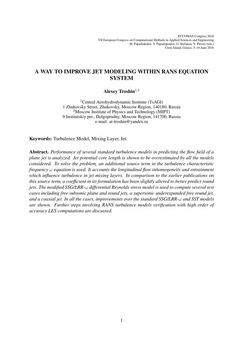
Computational domain scheme and boundary conditions (BCs) are shown in Figure 1 (scal-ing is not proportional). Soft Riemann invariants based BCs are specified on the left boundary(above the jet flow region) and on the upper half of the right boundary. On the lower part of theright boundary, extrapolation BCs are used to better predict the outflow of the jet. Symmetryplane is set at the top (to avoid incorrect entrainment flow patterns) and the bottom (which isjet centerplane). External boundaries are placed 200h away from the jet centerplane. No-slipBCs are set on the nozzle wall which length is equal to h. Ambient outer flow with relativevelocity u∞/u0 = 0.01 is specified in order to avoid instabilities due to interaction of soft BCswith stagnant air.
There are several published sets of experimental data on free subsonic plane jets. In thispaper, data on velocity distributions along the centerline are taken from [11, 12, 13, 14]. Ac-cording to them, jet potential core length Lini defined as the distance from the nozzle exit to thepoint where centerplane velocity is 0.99u0, lies in the range 5h ≤ Lini ≤ 6h.
2.3 Computational meshes and mesh convergence study
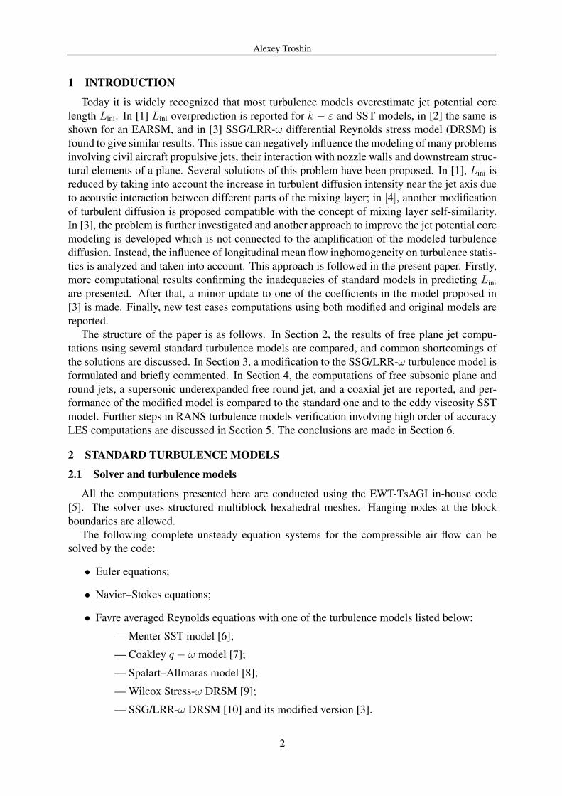
A set of three nested meshes has been generated containing approximately 60000, 15000,and 4000 cells. An overview and nozzle region of the coarse mesh are presented in Figure 2.Hanging nodes outside the jet region are clearly visible. They allow to significantly reduce thenumber of cells without affecting the accuracy of the results.
The fine mesh is designed to reproduce in details the mean flow in mixing layers (about 120cells across the turbulent zone) and shear region downstream the initial region of the jet (about140 cells per jet half-width). Nozzle boundary layer is resolved with 60 cells across it, the firstcell height in wall units being of the order of 1.
To study the mesh convergence, computations with SST turbulence model have been per-
3
Alexey Troshin
Rie
man
n B
C
Rie
man
n B
C
Ext
rapo
latio
n
Symmetry plane
Symmetry plane
Inle
t
Slip BC (Symmetry plane)No-slip BC
(jet region)
Figure 1: Computational domain scheme and boundary conditions of the plane jet test.
-50 0 50 100 150 200
0
20
40
60
80
100
120
140
160
180
200
0 2 4 6 8 10
0
2
4
6
8
Figure 2: An overview (left) and nozzle region (right) of the coarse mesh for the plane jet test.
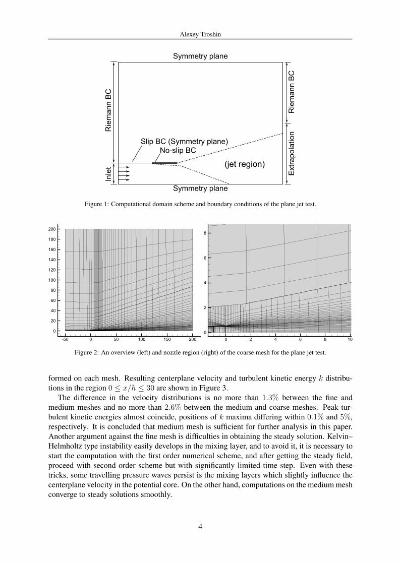
formed on each mesh. Resulting centerplane velocity and turbulent kinetic energy k distribu-tions in the region 0 ≤ x/h ≤ 30 are shown in Figure 3.
The difference in the velocity distributions is no more than 1.3% between the fine andmedium meshes and no more than 2.6% between the medium and coarse meshes. Peak tur-bulent kinetic energies almost coincide, positions of k maxima differing within 0.1% and 5%,respectively. It is concluded that medium mesh is sufficient for further analysis in this paper.Another argument against the fine mesh is difficulties in obtaining the steady solution. Kelvin–Helmholtz type instability easily develops in the mixing layer, and to avoid it, it is necessary tostart the computation with the first order numerical scheme, and after getting the steady field,proceed with second order scheme but with significantly limited time step. Even with thesetricks, some travelling pressure waves persist is the mixing layers which slightly influence thecenterplane velocity in the potential core. On the other hand, computations on the medium meshconverge to steady solutions smoothly.
4
Alexey Troshin
Figure 3: Centerplane velocity (left) and kinetic energy (right) distributions obtained on a set of nested meshes.1 — coarse mesh, 2 — medium mesh, 3 — fine mesh.
2.4 Results comparison
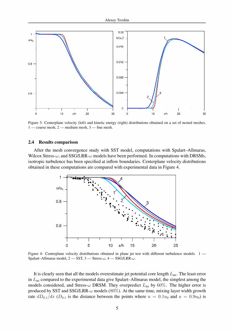
After the mesh convergence study with SST model, computations with Spalart–Allmaras,Wilcox Stress-ω, and SSG/LRR-ω models have been performed. In computations with DRSMs,isotropic turbulence has been specified at inflow boundaries. Centerplane velocity distributionsobtained in these computations are compared with experimental data in Figure 4.
Figure 4: Centerplane velocity distributions obtained in plane jet test with different turbulence models. 1 —Spalart–Allmaras model, 2 — SST, 3 — Stress-ω, 4 — SSG/LRR-ω.
It is clearly seen that all the models overestimate jet potential core length Lini. The least errorin Lini compared to the experimental data give Spalart–Allmaras model, the simplest among themodels considered, and Stress-ω DRSM. They overpredict Lini by 60%. The higher error isproduced by SST and SSG/LRR-ω models (80%). At the same time, mixing layer width growthrate dD0.1/dx (D0.1 is the distance between the points where u = 0.1u0 and u = 0.9u0) is
5
Alexey Troshin
predicted much better and lies within ±15% around experimentally observed value for all theturbulence models considered. Obtained values are collected in Table 1.
Data Lini/b dD0.1/dxexperiments 5− 6 0.14− 0.18
Spalart–Allmaras 9 0.17SST 10 0.15
Stress-ω 9 0.15SSG/LRR-ω 10 0.14
Table 1: Plane jet potential core lengths and mixing layer width growth rates predicted by different turbulencemodels.
It turns out that different classes of turbulence models, from one equation eddy viscositymodels to DRSMs, are affected by the same issue of overestimating Lini while correctly pre-dicting dD0.1/dx. This suggests an idea that mixing layer velocity profile is distorted such thatthe whole turbulent zone is “rotated” outwards the jet centerplane. In the following Section, amodification to the turbulence characteristic frequency ω equation is described which fixes themixing layer velocity profile and recovers the correct Lini in computations.
3 MODIFIED TURBULENCE MODEL
The ideas of the modification are given here in brief and consecutive derivation of the for-mulas is omitted because these questions were the subjects of another paper [3] where they aredescribed in details. The main goal of the current paper is to extend the number of test cases ofthe modified model and to more thoroughly assess its performance.
3.1 The idea of the modification
The first step of the SSG/LRR-ω model modification is recalibration of its coefficients inorder to obtain as accurate description of mixing layers as possible. During the coefficientstuning it appears that temporal mixing layer velocity profile [15] is easy to reproduce, but singlestream spatial mixing layer is a challenge. The process of tuning is described in [3]. The new“free stream” coefficient values using the designations of [10] are:
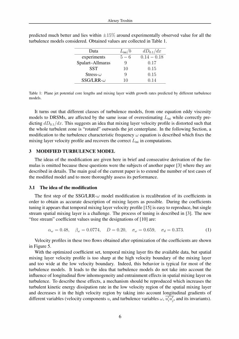
Velocity profiles in these two flows obtained after optimization of the coefficients are shownin Figure 5.
With the optimized coefficient set, temporal mixing layer fits the available data, but spatialmixing layer velocity profile is too sharp at the high velocity boundary of the mixing layerand too wide at the low velocity boundary. Indeed, this behavior is typical for most of theturbulence models. It leads to the idea that turbulence models do not take into account theinfluence of longitudinal flow inhomogeneity and entrainment effects in spatial mixing layer onturbulence. To describe these effects, a mechanism should be reproduced which increases theturbulent kinetic energy dissipation rate in the low velocity region of the spatial mixing layerand decreases it in the high velocity region by taking into account longitudinal gradients ofdifferent variables (velocity components ui and turbulence variables ω, u′iu′j , and its invariants).
6
Alexey Troshin
Figure 5: Velocity profiles in temporal (left) and single stream spatial (right) mixing layers after optimization ofthe SSG/LRR-ω model coefficients.
3.2 Modified ω equation
One possible form of taking into account the effects mentioned above is an additional sourceterm Iω in ω equation [3]. It can be written as
∂ρω
∂t+
∂
∂xk(ρωuk) = Sρω + ρIω,
Iω = −Cω3 0.03 th
(2Ωij
0.03ω4
∂ω
∂xi
∂k
∂xj
)ω2,
Ωij =1
2
(∂ui∂xj− ∂uj∂xi
), Cω3 = 20,
where Sρω are the standard diffusion and source terms in ω equation.Iω is a Galilean invariant, local source term which takes different signs at the opposite edges
of spatial mixing layers. In temporal mixing layer, it is zero. Recommended “free stream” Cω3
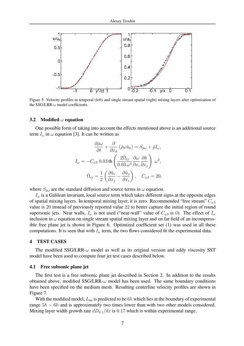
value is 20 instead of previously reported value 22 to better capture the initial region of roundsupersonic jets. Near walls, Iω is not used (“near-wall” value of Cω3 is 0). The effect of Iωinclusion in ω equation on single stream spatial mixing layer and on far field of an incompress-ible free plane jet is shown in Figure 6. Optimized coefficient set (1) was used in all thesecomputations. It is seen that with Iω term, the two flows considered fit the experimental data.
4 TEST CASES
The modified SSG/LRR-ω model as well as its original version and eddy viscosity SSTmodel have been used to compute four jet test cases described below.
4.1 Free subsonic plane jet
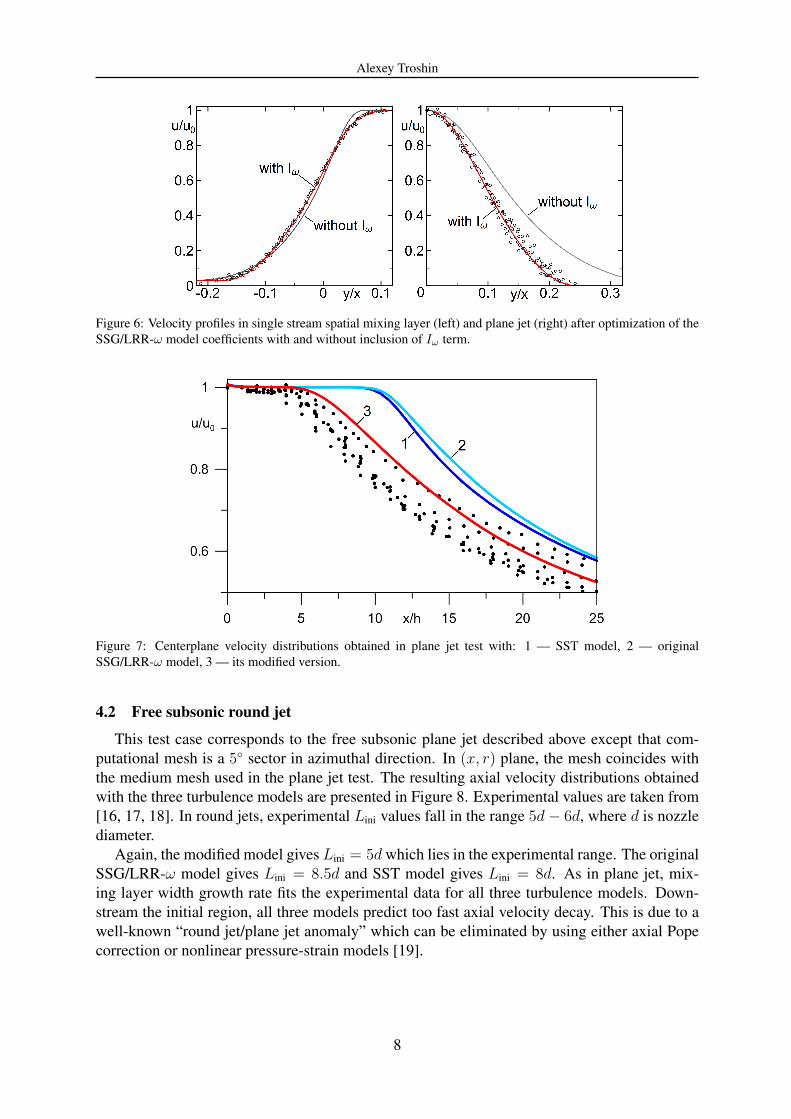
The first test is a free subsonic plane jet described in Section 2. In addition to the resultsobtained above, modified SSG/LRR-ω model has been used. The same boundary conditionshave been specified on the medium mesh. Resulting centerline velocity profiles are shown inFigure 7.
With the modified model, Lini is predicted to be 6hwhich lies at the boundary of experimentalrange 5h − 6h and is approximately two times lower than with two other models considered.Mixing layer width growth rate dD0.1/dx is 0.17 which is within experimental range.
7
Alexey Troshin
Figure 6: Velocity profiles in single stream spatial mixing layer (left) and plane jet (right) after optimization of theSSG/LRR-ω model coefficients with and without inclusion of Iω term.
Figure 7: Centerplane velocity distributions obtained in plane jet test with: 1 — SST model, 2 — originalSSG/LRR-ω model, 3 — its modified version.
4.2 Free subsonic round jet
This test case corresponds to the free subsonic plane jet described above except that com-putational mesh is a 5 sector in azimuthal direction. In (x, r) plane, the mesh coincides withthe medium mesh used in the plane jet test. The resulting axial velocity distributions obtainedwith the three turbulence models are presented in Figure 8. Experimental values are taken from[16, 17, 18]. In round jets, experimental Lini values fall in the range 5d− 6d, where d is nozzlediameter.
Again, the modified model gives Lini = 5dwhich lies in the experimental range. The originalSSG/LRR-ω model gives Lini = 8.5d and SST model gives Lini = 8d. As in plane jet, mix-ing layer width growth rate fits the experimental data for all three turbulence models. Down-stream the initial region, all three models predict too fast axial velocity decay. This is due to awell-known “round jet/plane jet anomaly” which can be eliminated by using either axial Popecorrection or nonlinear pressure-strain models [19].
8
Alexey Troshin
Figure 8: Axial velocity distributions obtained in round jet test with: 1 — SST model, 2 — original SSG/LRR-ωmodel, 3 — its modified version.
4.3 Underexpanded free round jet
In this test, a cold free supersonic round air jet has been modeled. It was studied experi-mentally at ITAM SB RAS [20]. The jet issues from a converging nozzle with Mach numberat the exit equal to 1. Nozzle pressure ratio is 2.8. Nozzle diameter d based Reynolds numbernumber Red = ued/νe is 8.5× 10⁵, where parameters with subscript “e” are taken at the nozzleexit. Turbulence level at the nozzle exit Tue is taken to be 0.9% to reproduce the experimentalconditions.
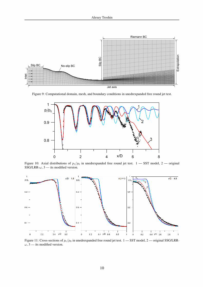
An overview of the computational domain, mesh, and boundary conditions is shown in Fig-ure 9. When generating the mesh, its density has been taken to be approximately the same asin medium mesh in free subsonic plane jet, which had been shown to produce mesh convergedsolutions.
In Figure 10, axial distributions of relative Pitot pressure pt/p0, where p0 is the total pressurein the core of the nozzle, are shown. SST and original SSG/LRR-ω models capture the first4 cells of the jet, after which they do not predict experimental pt fall. Moreover, SST modelunderpredicts the amplitude of pt oscillations at x/d > 5. The modified SSG/LRR-ω modelcaptures 5 jet cells and pt fall at x/d > 5, which fits the experimental data better.
In Figure 11, three cross-sections of pt/p0 obtained in computations are compared with theexperimental data. SST and original SSG/LRR-ω models give similar results predicting toosharp high velocity boundary of the mixing layer. The modified SSG/LRR-ω model makemixing layer smoother in this region and captures the experimental behavior of Pitot pressure.
4.4 Coaxial jet
This flow was also studied experimentally at ITAM SB RAS. Now it is one of the tests inFirst TILDA Workshop on Industrial LES & DNS (2016). A cold free air jet issues from a dual-stream round nozzle. The inner contour is subsonic with nozzle pressure ratio NPR1 = 1.72and Mach number at the exit M1 = 0.8. The outer contour is supersonic with NPR2 = 2.25(underexpanded flow) andM2 = 1.0. Outer contour diameterD based Reynolds number ReD =u2D/ν2 is equal to 2.9× 10⁶.
Computational mesh near the nozzle is shown in Figure 12. As in previous test, mesh density
9
Alexey Troshin
Riemann BC
Ext
rapo
latio
n
Slip
BC
Inle
t
No-slip BC
Jet axis
Slip BC
Figure 9: Computational domain, mesh, and boundary conditions in unedrexpanded free round jet test.
Figure 10: Axial distributions of pt/p0 in unedrexpanded free round jet test. 1 — SST model, 2 — originalSSG/LRR-ω, 3 — its modified version.
Figure 11: Cross-sections of pt/p0 in unedrexpanded free round jet test. 1 — SST model, 2 — original SSG/LRR-ω, 3 — its modified version.
10
Alexey Troshin
has been taken to be approximately the same as in medium mesh in free subsonic plane jet toget mesh converged solutions. In this test, it contains approximately 150000 cells.
Figure 12: Mesh in coaxial jet test. Every second mesh line is shown.
In Figure 13, three computed cross-sections of pt/p0, where p0 is the total pressure in the airsupply of the outer contour, are compared with the experimental data. Longitudinal coordinateaxis x origin is at the tip of the central body. As clearly seen from the experimental data,boundary layers at the walls of the outer contour are much thicker than in computations. Infact, their traces collapse already at x/D = 0.08. This leads to lower peak pt values at y/D ≈0.3 than in computations. SST model predicts a small region of pt decrease at y/D ≈ 0.2downstream the position x/D = 0.80 which is absent both in experiments and in computationsusing DRSMs. On the other hand, wake intensity behind the central body is overpredictedby all the models considered. This is an interesting issue to investigate in the future. Apartfrom this discrepancies, the overall agreement between the computations and the experimentis satisfactory. The modified SSG/LRR-ω model predicts a different velocity profile in theouter mixing layer which seems to be realistic since similar behavior allowed to better fit theexperimental data in the previous tests.
5 FURTHER STEPS: LES BASED VALIDATION
As has been shown in paper, the modified model improves modeling accuracy of the jet flowsconsidered in the paper. However, several questions are still open, some of them are:
• Are there other, maybe simpler, forms of additional source term in ω equations whichplay the same role as Iω used in the paper? If there are, which one to prefer?
• How to further modify turbulence model equations to better capture the decay of turbulentwakes, e.g. central body wake in the coaxial jet test?
• How do mixing layers develop when they originate from thick boundary layers? Are thereany specific features? Does Iω term needs a correction in this case? This can be studied ina series of coaxial jet test computations with correct boundary layers in the outer contour.
11
Alexey Troshin
Figure 13: Cross-sections of pt/p0 in coaxial jet test. 1 — SST model, 2 — original SSG/LRR-ω, 3 — its modifiedversion.
Nowadays, there is strong progress in developing and validating the high order LES tech-niques, among which is Discontinuous Galerkin based LES [21]. These techniques are capableof accurately capturing turbulence phenomena in the range of scales, and it looks natural to usethese capabilities for term-by-term validation and tuning of RANS turbulence models.
As the next step for the research presented in the paper, we plan to conduct LES basedcomputations of the coaxial jet to get answers to at least some of the questions listed above. Wehave developed a new in-house code with the following features:
• High spatial order Discontinuous Galerkin method with up to piecewice cubic polynomi-als.
• Explicit time discretization (multistage Runge–Kutta schemes of up to 4th order) withfractional time stepping technique.
• Complete compressible LES equation system with Smagorinsky subgrid scale model.
• MPI parallelism with efficient scalability on up to ∼ 104 cores.
The data obtained in LES computations will allow to extract distributions of individual termsin Reynolds stress and ω equations. They will be compared to the data in RANS computationsto improve the engineering models for different terms in RANS turbulence models.
6 CONCLUSIONS
It is shown that different standard turbulence models, from linear eddy viscosity modelsto DRSMs, incorrectly predict jet potential core length. SSG/LRR-ω DRSM is recalibratedand supplemented by an additional source term in the turbulence characteristic frequency ωequation which accounts the longitudinal flow inhomogeneity and entrainment. These effectsinfluence turbulence in jet mixing layers and change its velocity profile. Four jet test cases areconsidered, in all of which the modified model improves the accuracy of flow field predicionover the standard models examined in the paper.
Theoretical part of the study was supported by RFBR, research project No. 16-38-00760.Computations presented in the paper were supported by the Ministry of Education and Sci-
[1] W.A. Engblom, N.J. Georgiadis, A. Khavaran, Investigation of variable-diffusion turbu-lence model correction for round jets. 11th AIAA/CEAS Aeroacoustics Conference, Mon-terey, California, May 23-25, 2005.
[2] N.J. Georgiadis, D. Papamoschou, Computational investigations of high-speed dual-stream jets. 9th AIAA/CEAS Aeroacoustics Conference and Exhibit, Hilton Head, SouthCarolina, May 12-14, 2003.
[3] A.I. Troshin, A turbulence model taking into account the longitudinal flow inhomogene-ity in mixing layers and jets. 6th European Conference for Aerospace Sciences, Krakow,Poland , June 29 - July 3, 2015.
[4] A.I. Troshin, A turbulence model with variable coefficients for calculating mixing layersand jets. Fluid Dynamics, 47, No. 3, 320–328, 2012.
[5] V. Neyland, S. Bosniakov, S. Glazkov, A. Ivanov, S. Matyash, S. Mikhailov et al., Concep-tion of electronic wind tunnel and first results of its implementation. Progress in AerospaceSciences, 37, No. 2, 121–145, 2001.
[6] F.R. Menter, M. Kuntz, R. Langtry, Ten years of industrial experience with the SST turbu-lence model. Turbulence, Heat and Mass Transfer, 4, 625–632, 2003.
[7] T.J. Coakley, Turbulence modeling methods for the compressible Navier-Stokes equations.AIAA 16th Fluid and Plasma Dynamics Conference, Danvers, Massachusetts, July 12-14,1983.
[8] P.R. Spalart, S.R. Allmaras, A one-equation turbulence model for aerodynamic flows. 30thAerospace Sciences Meeting & Exhibit, Reno, Nevada, January 6-9, 1992.
[10] R.-D. Cecora, R. Radespiel, B. Eisfeld, A. Probst, Differential Reynolds-stress modelingfor aeronautics. AIAA Journal, 53, 739–755, 2015.
[11] E. Gutmark, I.J. Wygnanski, The planar turbulent jet. Journal of Fluid Mechanics, 73,465–495, 1976.
[12] B.R. Ramaprian, M.S. Chandrasekhara, LDA measurements in plane turbulent jets. Jour-nal of Fluids Engineering, 107, 264–271, 1985.
[13] M. Alnahhal, Th. Panidis, The effect of sidewalls on rectangular jets. Experimental Ther-mal and Fluid Science, 33, 838–851, 2009.
[14] R.C. Deo, J. Mi, G.J. Nathan, The influence of Reynolds number on a plane jet. Physicsof Fluids, 20, 075108, 2008.
[15] J.H. Bell, R.D. Mehta, Development of a two-stream mixing layer from tripped and un-tripped boundary layers. AIAA Journal, 28, 2034–2042, 1990.
13
Alexey Troshin
[16] H.J. Hussein, S.P. Capp, W.K. George, Velocity measurements in a high-Reynolds-number, momentum-conserving, axisymmetric, turbulent jet. Journal of Fluid Mechanics,258, 31–75, 1994.
[17] J.C. Lau, P.J. Morris, M.J. Fischer, Measurements in subsonic and supersonic free jetsusing a laser velocimeter. Journal of Fluid Mechanics, 93, 1–27, 1979.
[18] J. Bridges, M. Wernet, Establishing consensus turbulence statistics for hot subsonic jets.16th AIAA/CEAS Aeroacoustics Conference, Stockholm, Sweden, June 7-9, 2010.
[19] K. Hanjalic, B. Launder, Modelling turbulence in engineering and the environment:second-moment routes to closure. Cambridge University Press, 2011.
[21] F. Bassi, L. Botti, A. Colombo, A. Crivellini, A. Ghidoni, A. Nigro, S. Rebay, Time in-tegration in the Discontinuous Galerkin code MIGALE - unsteady problems. NumericalFluid Mechanics and Multidisciplinary Design, 128, 205–230, 2015.