A way to synchronize models with seismic faults for earthquakeforecasting: Insights from a simple stochastic model
Álvaro González a,⁎, Miguel Vázquez-Prada b, Javier B. Gómez a, Amalio F. Pacheco b
a Departamento de Ciencias de la Tierra, Universidad de Zaragoza, C./ Pedro Cerbuna, 12. 50009 Zaragoza, Spainb Departamento de Física Teórica and BIFI, Universidad de Zaragoza, C./ Pedro Cerbuna, 12. 50009 Zaragoza, Spain
Received 5 August 2005; received in revised form 11 November 2005; accepted 25 March 2006Available online 23 June 2006
Abstract
Numerical models are starting to be used for determining the future behaviour of seismic faults and fault networks. Their finalgoal would be to forecast future large earthquakes. In order to use them for this task, it is necessary to synchronize each model withthe current status of the actual fault or fault network it simulates (just as, for example, meteorologists synchronize their models withthe atmosphere by incorporating current atmospheric data in them). However, lithospheric dynamics is largely unobservable:important parameters cannot (or can rarely) be measured in Nature. Earthquakes, though, provide indirect but measurable clues ofthe stress and strain status in the lithosphere, which should be helpful for the synchronization of the models.
1. Introduction: data assimilation in numerical faultmodels
Numerical models are now frequently used to simulatethe seismic behaviour of faults (e.g. Kato and Seno, 2003;Fitzenz and Miller, 2004; Kuroki et al., 2004) and fault
networks (e.g. Ward, 2000; Hashimoto, 2001; Robinsonand Benites, 2001; Rundle et al., 2001; Soloviev andIsmail-Zadeh, 2003; Robinson, 2004; Rundle et al., 2004,2006). In these models, fault planes separate lithosphericblocks that are strained at specific rates, and sudden slips(earthquakes) are generated by the faults according tocertain friction and/or rupture laws. Although no com-pletely realistic dynamical model presently exists, thesesimulations are now sufficiently credible to begin to play asubstantial role in scientific studies of earthquake
320 Á. González et al. / Tectonophysics 424 (2006) 319–334
probability and hazard (Ward, 2000). The final goals of thenumerical modelling of seismicity are not different from,for example, the goals of numerical models of theatmosphere. A good model should be able to:
(1) reproduce the general characteristics of thesystem,
(2) mimic the state of the system at the presentmoment, and
(3) forecast the future evolution of the system.
Most numerical models of seismicity have beendesigned to achieve the first goal, by reproducinggeneral characteristics of earthquakes such as their size–frequency distribution (e.g. Bak and Tang, 1989; Olamiet al., 1992; Dahmen et al., 1998; Preston et al., 2000;Vázquez-Prada et al., 2002), or the generation ofaftershocks and foreshocks (e.g. Hainzl et al., 1999).When a model is designed this way, it is left to evolvefreely according to its rules, and all that is checked iswhether the overall results of the model are similar to theobservations made in Nature.
The second goal requires data assimilation, that is, theprocess of absorbing and incorporating observed infor-mation into themodel. By this process, themodel is tunedand synchronized, at least partially, with the real system ittries to simulate. In a meteorological model, data ofatmospheric pressure, temperature, humidity, cloudcover, precipitation, etc. measured in a given momentat different locations and heights can be included. Withthis procedure, the model becomes a reasonably goodrepresentation of the atmosphere at that moment. Then itcan be used to calculate the probable future atmosphericevolution (i.e. the third goal cited above).
Seismic data assimilation poses greater problemsthan its meteorological equivalent. This explains (atleast partially) the relative delay in developing reliableforecasts of large earthquakes. The inner workings ofboth the atmosphere (Houghton, 2002) and thelithosphere (Goltz, 1997; Turcotte, 1997; Keilis-Borok, 2002) are complex and chaotic, so they areinherently difficult to forecast. However, while meteor-ologists can probe the atmosphere every day at differentplaces and heights (and assimilate the obtained data intheir models in near real-time), lithospheric variables ofparamount importance, such as the stress and strain, canbe measured only in certain places, and not at any time:earthquakes have unobservable dynamics (e.g. Rundleet al., 2003). For example, the best current compendiumof stress magnitudes and directions in the lithosphere isthe World Stress Map (Zoback, 1992; Reinecker et al.,2005), whose entries are point static time-averaged
estimates of maximum and minimum principal stressesin space. And the direct measurements of stress onactive fault zones at depth are still scarce (e.g. Ikeda etal., 2001; Tsukahara et al., 2001; Yamamoto and Yabe,2001; Hickman and Zoback, 2004; Boness and Zoback,2004). The numerical models would need better spatialand temporal information of stress, both more abundantand more systematically collected than that currentlyavailable (Rundle et al., 2004). It is thus necessary toseek ways to tune and synchronize the models withmore abundant observable data.
A first step of data assimilation in models ofearthquake faults is to introduce information regardingthe topology (that is, the shape and location) of theactive faults and their long-term behaviour. Forexample, the long-term fault slip rate, and the averagerecurrence interval of the largest earthquakes in the faultcan be estimated from paleoseismological studies andshould be included in the models (Grant and Gould,2004). Examples of this approach are the works of Ward(2000), Robinson (2004) and Rundle et al. (2006). Thesurface deformation measured via Global PositioningSystem (GPS) networks and by Synthetic ApertureRadar Interferometry (InSAR) can also constitute inputdata for the fault models (Rundle et al., 2004).Earthquakes themselves are indeed the most obviousobservable events of lithospheric dynamics, and couldprovide the most detailed data available to assimilate inthe models, but how? The earthquake rupture area couldbe an important clue.
The rupture area and slip distribution in real earth-quakes can be very complex (Sieh, 1996; Kanamori andBrodsky, 2004), but can be estimated in a variety ofways. The slip distribution can be calculated byinverting the observed seismic waveforms (Kanamoriand Brodsky, 2004) or tsunami waveforms (e.g. Taniokaet al., 2004; Baba and Cummins, 2005), and/or bygeodetic modelling of ground displacement (Yabuki andMatsuura, 1992). Some earthquakes produce surfaceruptures, which are useful for estimating the rupture area(Stirling et al., 2002). Although most surface rupturesoccur in large shocks, with magnitudes larger than about6, they have been reported for earthquakes withmagnitudes down to 2.5 (see the compilation of historicearthquakes with surface rupture by Yeats et al., 1997,pp. 473–485). Also, the rupture area can be estimatedfrom the seismic moment (calculated from the amplitudespectra of seismic waves; Scholz, 2002; Kanamori andBrodsky, 2004), or from the moment magnitude (Wellsand Coppersmith, 1994; Stirling et al., 2002; Dowrickand Rhoades, 2004). Frequently the location of earlyaftershocks is used to determine the rupture area of the
321Á. González et al. / Tectonophysics 424 (2006) 319–334
mainshock (Wells and Coppersmith, 1994), although theaftershock zone tends to grow with time (Kisslinger,1996) and is not necessarily a good indicator of that area(Yagi et al., 1999).
Complex models with realistic fault topology areable to reproduce the rupture area and co-seismic slipof past earthquakes. It is thus possible to force themodel to reproduce the rupture of a past earthquake,and let it evolve from that moment onwards to seewhat could happen in the future. For example, Ward(2000) developed a model including the network ofmain faults in the San Francisco Bay Area (California).He forced the model to reproduce the San AndreasFault surface co-seismic slip of the 1906 San Franciscoearthquake, and let it evolve freely from thatearthquake onwards, in an attempt to simulate theprobable sequence of earthquake ruptures during thenext 3000 years.
But considering only the data of the largestearthquake in the series is probably not sufficient toproperly synchronize the model. Complex and chaoticsystems are very sensitive to the initial conditions. Theinformation regarding only one event probably does notsufficiently constrain the initial conditions, and thecalculated evolution will probably be a particular caseof a large range of possible outcomes. Will thispanorama improve by forcing the model to reproduceall the observed earthquake ruptures, including thesmall ones? Probably yes. To check whether this ideaworks, at least to forecast synthetic seismicity, is thepurpose of this paper. The number of recorded largeearthquakes is relatively scarce, especially in individualfaults (where the recorded series very rarely includesten large events). This hampers the ability to charac-terize statistically the effectiveness of any forecastingmethod. Synthetic earthquake catalogues, on the otherhand, can be as long as desired. This enables toascertain, with robust statistics, whether a forecastingstrategy could be useful, before endeavouring to applyit to real seismicity.
In the following sections, our goal will be to forecastthe largest earthquakes generated by the minimalistmodel, a simple numerical fault model. We will showthat when all the earthquake ruptures generated by thismodel are imposed on other, similar models, thesebecome partially synchronized with the former. We usethem to declare alarms that efficiently mark theoccurrence of the largest shocks in the first model.The results are much better than those obtained withother strategies that consider only the earthquake series.The model, albeit simple, is stochastic (it involvesrandomness), so its efficient forecasting is not trivial.
We will describe how this stochasticity can be dealtwith, by using an approach similar to the so-calledensemble forecasting used in Meteorology (Palmer etal., 2005). The method could be used in other moredetailed and realistic models (stochastic or not) to testour general conclusion: that they might be partiallysynchronized with actual faults by being forced toreproduce the series of observed earthquake ruptures.
In the next section we describe the model and itsproperties. Then, we outline the general scheme ofprediction and the forecasting strategies used asreference to assess the merits of any other predictivemethod in the model. Finally, the method based onpartial synchronization is explained and its possibleutility discussed.
2. The minimalist model
The minimalist model is the numerical model whoselargest earthquakes we will try to forecast. It wasintroduced in a previous work (Vázquez-Prada et al.,2002), and has mainly two, apparently contradictory,advantages for the purpose of this paper: it is simplebut, at the same time, it is difficult to forecast. Becauseit is simple, several of its properties can be derivedanalytically, and it can be characterized in detail withnumerical simulations which do not require animpractical amount of computer time. Because it isstochastic, it is difficult to forecast, so the results wewill obtain here are not trivial. In the followingparagraphs we will explain how the model works, andwhat are its main properties, comparing them with thoseof actual faults.
2.1. How the model works
The model is a simple (hence its name) cellularautomaton. Cellular automata are frequently used tomodel seismic faults. In these models, the fault plane isdivided into a grid of cells (each cell representing afraction of the fault area), and the time evolves indiscrete time steps. Each cell's state is updated at eachtime step according to rules that usually depend on thestate of the cell or that of its neighbors in the previoustime step. These rules can be designed according tocertain friction laws (Ben-Zion, 2001), stress transfer(Olami et al., 1992; Hainzl et al., 1999; Preston et al.,2000), and the mechanical effects of fluids (Miller et al.,1999). In the minimalist model, as well as in other verysimple cellular automata (e.g. Newman and Turcotte,2002; González et al., 2005), these details are ignored:the model is driven stochastically, there are only two
322 Á. González et al. / Tectonophysics 424 (2006) 319–334
possible states for each cell, and the earthquakes aregenerated according to simplified breaking rules.
Let us now explain the simplified view of earthquakegeneration that the model tries to sketch. In actual faults,the regional stress strains the rock blocks of the fault,making portions (patches) of the fault plane to becomemetastable. That is, they are static, but store enoughelastic energy to propagate an earthquake rupture oncetriggered. Different processes (for example, fault creep—aseismic slip— and plastic deformation) dissipatestress along the fault plane, so stress is not directlyconverted into elastic strain. Earthquakes rupture someof the metastable patches of the fault, that then becomestable, thus relieving strain. The hypocentre of anearthquake is usually located in a particularly strongpatch of the fault plane, called “asperity” (Kanamori andStewart, 1978; Aki, 1984; Das, 2003; Lei et al., 2003).Asperities appear to be persistent features whereearthquake ruptures start once and again (Aki, 1984;Okada et al., 2003). Once the rupture starts, itpropagates along the fault plane until it arrives at apatch of the fault that is not sufficiently strained. Thenthe rupture cannot propagate further, and is arrested. Therelatively stable patch that is not sufficiently strainedand that arrests the rupture is called the “barrier” (Dasand Aki, 1977; Aki, 1984; Das, 2003).
The model, depicted in Fig. 1, sketches these featuresas follows. It divides the plane of a fault into an array ofN equal cells, each denoted by an index i. In previouspapers (Vázquez-Prada et al., 2002, 2003; López-Ruiz
Fig. 1. The minimalist model as a sketch of a seismic fault. The faultplane is divided into an array of N equal cells, denoted with an index i,1≤ i≤N. The increase of regional stress is represented by the randomaddition of “stress particles” to the cells. Earthquake ruptures start at anasperity, the cell i=1, when a stress particle arrives to it. The rupturepropagates through all the consecutive metastable cells (occupied byparticles). The rupture area is k, the number of cells broken. The figuredepicts an earthquake with k=3.
et al., 2004; Gómez and Pacheco, 2004; González et al.,2004), this array was drawn vertically, in order tosimplify its description. Here the model will be drawnhorizontally, in order to sketch the fault plane in a waymore similar to that of actual faults (which are usuallylonger along the strike than along the dip). Some othercellular automaton models discretize the fault plane ina similar way (e.g. Rundle et al., 2004, 2006). Theparameter N is the only one that can be changed in themodel. The cells can only be in one of two states:“empty” (stable) or “occupied” (metastable). The stateof the model at each time step can be described simplyby stating which cells are occupied and which are not.The increase of regional stress, as in other simplemodels (Bak and Tang, 1989; Castellaro and Mulargia,2001; Newman and Turcotte, 2002; González et al.,2005), is represented by the random addition of “stressparticles”. This randomness is a way of dealing withthe complex stress increase in actual faults. At eachtime step, one cell is selected randomly, and a newparticle arrives on it. That is, each cell has the sameprobability, 1/N, of receiving the new stress particle. Ifthe chosen cell is empty, the particle “occupies” it. Thismeans that the regional stress has produced enoughstrain on that cell to make it metastable. If the cell isalready occupied, that stress particle is lost; this isanalogous to stress dissipation on the fault plane. Thetotal number of occupied cells represents the totalelastic strain on the fault.
In the model, we assume that there is only one,persistent, asperity: the first cell, i=1, placed at one endof the array. This option is chosen because it simplifiesthe analytical description of the model. When a stressparticle fills cell i=1, a rupture starts there, andpropagates through all the consecutive metastable cellsuntil it is arrested by a stable cell. That is, if all thesuccessive cells i=1 to i=k are occupied, and cell k+1 isempty, then the effect of the earthquake is to empty allthe cells from i=1 to i=k. The other cells, i>k remainunaltered. The cell k+1 is a barrier: it is empty (stable),so the rupture cannot propagate through it. The size(rupture area) of the earthquake is k, the number of cellsbroken in the synthetic earthquake. Thus, the earthquakesize in the model is discrete, 1≤k≤N. Earthquakes, inpractice, are instantaneous in the model (they do not lastfor any time step). This represents the fact thatearthquake ruptures are, indeed, much faster than theslow stress loading represented by the addition ofparticles.
The random addition of particles is what makes themodel stochastic. It also determines the rate at whichearthquakes occur in the model. At each time step,
Fig. 2. The number of occupied cells in a minimalist model withN=20, for ten seismic cycles. This number is analogous to the totalelastic strain accumulated in the fault. Sudden drops correspond toearthquakes. Each seismic cycle ends with an earthquake of size N.
323Á. González et al. / Tectonophysics 424 (2006) 319–334
independently of the previous earthquake history, thereis a probability 1/N for the incoming stress particle toarrive at cell i=1 and start an earthquake. Thus anearthquake, on average, occurs every N steps. The timebetween any two consecutive earthquakes is purelyrandom (exponentially distributed, with rate 1/N).
The cellular-automaton approach of this model issimilar to that of the “forest fire” models, in whichclusters of interconnected occupied cells (“trees”)“burn” and are reset to empty when they are randomlystruck by “lightning” (Drossel and Schwabl, 1992;Henley, 1993). The utility of this kind of models forearthquake physics has been noted by Rundle et al.(2003). In the minimalist model there is no random“lightning”: the clusters of interconnected metastablesites are only emptied if they are connected to the celli=1 and if this fails.
2.2. Main properties of the model
The minimalist model, because of its extremesimplicity, lacks the detailed description of the seismicprocess that a fully dynamical model can display. Forexample, it does not include the effects of fault friction,elastic stress transfer, or the role of fluids that morecomplex models can take into account. However, itspontaneously displays several properties that arecomparable to those of actual faults, outlined as follows:
(1) Earthquake size–frequency distribution. It is ofthe characteristic earthquake type (Wesnousky etal., 1983; Schwartz and Coppersmith, 1984;Youngs and Coppersmith, 1985; Wesnousky,1994), observed in seismic faults with simpletraces (Stirling et al., 1996) and in othernumerical models if the fault plane is homoge-neous (e.g. Rundle and Klein, 1993; Main, 1996;Dahmen et al., 1998; Steacy and McCloskey,1999; Moreno et al., 1999; Hainzl and Zöller,2001; Heimpel, 2003; Zöller et al., 2005). In thisdistribution there is a relative excess of events(called characteristic earthquakes) which breakthe whole fault or most of it. In the model, theyare the earthquakes with size N, and will be theevents to forecast. The Gutenberg–Richter distri-bution (Ishimoto and Iida, 1939; Gutenberg andRichter, 1944, 1954) observed in regionalseismicity (which includes contributions frommany faults) can be reproduced adding up theseismicity of an ensemble of minimalist modelswhose sizes (N) are distributed as in actual faults(López-Ruiz et al., 2004).
(2) Duration of the earthquake cycle. The earthquakecycle of a fault is the time interval between twoconsecutive characteristic earthquakes (e.g.Scholz and Gupta, 2000). The statistical distribu-tion of these intervals in the model is similar to theobserved in seismic faults (Gómez and Pacheco,2004). The distribution of time intervals betweenconsecutive earthquakes of any size in the modelis exponentially distributed. However, if only thecharacteristic earthquakes are considered, thedistribution is not exponential. This is becausethe maximum possible size of an event dependson the size of the previous event and the timeelapsed since it occurred. This is commented inthe next paragraph.
(3) Stress shadow. When a fault generates a largeearthquake, the elastic strain is reduced, and aminimum time has to elapse until the fault, byslow tectonic deformation, accumulates enoughstrain to generate another large earthquake. Thiseffect is called stress shadow (Harris, 2000). In theminimalist model there is a stress shadow: if anevent of size k takes place, at least k time stepshave to elapse until another event of that size canoccur.
(4) Pattern of strain loading. In actual faults, thestrain increases rapidly just after a large earth-quake, and then more slowly (Michael, 2005). Inthe model, the total elastic strain is represented bythe occupation (the total number of occupied cells,Fig. 2), which has a similar pattern. Just after alarge earthquake, there are fewer occupied cells,so it is more probable for the incoming particles toland on empty cells, and the occupation growsfaster than later on (Fig. 2).
(5) Seismic quiescence. The model displays seismicquiescence (absence of earthquakes) before the
324 Á. González et al. / Tectonophysics 424 (2006) 319–334
characteristic events. Once N−1 cells (from i=2to i=N) become occupied, the occupation reachesa plateau (Fig. 2) and, on average, N time stepshave to elapse until the next earthquake (which isthe characteristic one) occurs. Seismic quiescencehas been observed preceding many large earth-quakes (e.g. Wyss and Habermann, 1988; Scholz,2002), although in other cases the opposite effect(increased activity) has been observed (e.g.Bowman et al., 1998; Reasenberg, 1999; Tiampoet al., 2002). The minimalist model does not showthis last behaviour.
3. General scheme of forecasting
In this section we will explain the general frameworkfor the forecasting of the largest earthquakes in themodel. As a first remark, we have to consider that themodel is stochastic, so it is not predictable with absoluteprecision. Only simple deterministic systems are fullypredictable. The evolution of complex systems, such asthe atmosphere or the lithosphere (even if it weredeterministic) is very sensitive to the initial conditions.As these complex systems cannot be fully characterized,they turn out not to be fully predictable either.
Earthquake prediction (e.g. Keilis-Borok, 2002;Keilis-Borok and Soloviev, 2003; Rundle et al., 2003),as well as some atmospheric predictions (Mason, 2003),is frequently regarded as a binary forecast: one has todecide whether a large earthquake is going to occur ornot, in a certain time-space window, instead ofcalculating the exact probability of this event. In thisbinary-forecasting approach, an “alarm” is declaredwhen a large earthquake is expected. If it takes placewhen the alarm is on, the outcome is a successfulforecast. If it takes place when the alarm is off, there hasbeen a prediction failure. If the alarm was declaredduring a certain period, but the expected earthquake didnot happen, that constitutes a false alarm.
Note that for using this approach it is necessary todefine precisely what the target earthquakes are thatwe wish to forecast. Usually they are defined as thosewith a magnitude larger than a given threshold, bothwhen dealing with actual earthquakes (e.g. Keilis-Borok and Soloviev, 2003; Rundle et al., 2003) orwith synthetic ones (e.g. Pepke and Carlson, 1994;Hainzl et al., 2000). In the minimalist model, it isnatural to choose as target events the characteristicearthquakes (size k=N), as they mark a distinct peakin the size–frequency diagram, being much morefrequent than other large earthquakes (Vázquez-Pradaet al., 2002, 2003).
Away to quantify the forecasting ability of a certainstrategy is to compute the fraction of errors, fe, and thefraction of alarm time, fa (Molchan, 1997). Given acertain time series of the model, fe is the ratio of the totalnumber of prediction failures to the total number oftarget events. And fa is the ratio of the total time duringwhich the alarm was on to the total duration of the timeseries. The fraction of false alarms, ff, is included in fa,and is the ratio of the total duration of false alarms to thetotal duration of the time series.
Of course, a good forecasting strategy should rendersmall fa, fe and ff. However, as a general rule, a strategythat renders low fe tends to produce large fa and ff.Dealing with real seismicity, both a failure and an alarmare costly. Eventually, decision-makers would need toconsider what is less costly: to predict most of thedangerous earthquakes, but declaring many alarms, or todeclare fewer alarms but failing the forecast of morelarge shocks (Molchan, 1997). Depending on the trade-off between costs and benefits, one should try tominimize a loss function, L, that can depend on fa, fe and/or ff.
In the next section, we will describe the forecastingstrategies that will be used to compare the merits of thenew strategy proposed in this paper, based onsynchronizing models between themselves. In the firstof the subsections we will indicate the loss function wewill try to minimize in the forecasting of the model.
4. Forecasting strategies for comparison
We describe here three forecasting strategies, basedon the earthquake series, that we will use to asses themerits of the new strategy described later in this paper.The first two strategies (the random guessing strategyand the so called reference strategy) can be used in anysystem. The third is specific to the minimalist model,and serves to ideally determine its maximum theoreticalpredictability.
4.1. Random guessing strategy
In this strategy, the alarm is randomly turned on andoff. It is simple to apply this strategy to any cellularautomaton model. Here, in each time step, the alarm ison with a probability p. As a result, the alarm will be onduring a fraction p of time steps ( fa=p). When the targetearthquake finally occurs in a certain time step, therewill be a probability p for the alarm to be on. Thus, onaverage, a fraction p of target earthquakes will bepredicted, and a fraction fe=1−p will be predictionfailures, so fa+ fe=1. This strategy has two trivial cases:
Fig. 3. Loss function (L) obtained with the different forecastingmethods used in this paper, for various system sizes (2≤N≤20). Arandom guessing strategy would render L=1 for any N, while L=0would mean a perfect prediction. The shadowed zone is unattainablefor any forecasting strategy used in the minimalist model, and thestrategy that marks its upper limit is called “Ideal”. The “Reference”strategy is based only on the series of the largest earthquakes in themodel. The three strategies labelled “Clones” are based on thesynchronization of models with the minimalist model whose largestearthquakes we try to forecast.
325Á. González et al. / Tectonophysics 424 (2006) 319–334
if the alarm is always on ( fa=1), all the targetearthquakes are “forecasted” ( fe=0). Conversely, ifthe alarm is always off ( fa=0), we fail to predict any ofthem.
To be statistically significant, any forecastingstrategy must render better results than a randomguess. A natural way to measure this improvement isto consider the loss function L= fa+ fe. Then, L=1means that the strategy performs as a random guess,and L=0 means a perfect prediction. If L>1, thestrategy is performing exactly the opposite to how itshould. Thus, the exact reverse strategy should beconsidered, and this will provide the opposite results( fa′=1− fa, and fe′=1− fe).
4.2. Reference strategy
Of course, the random guessing strategy depictedabove is only useful as a baseline, but does not serve toprovide a real significant forecast. In this subsection wedescribe the simplest meaningful forecasting strategyone can consider for any system. This will be called thereference strategy, and any forecasting procedure morecomplex than this should render better results.
The reference strategy consists simply in declaring analarm some time after each target event, and maintainingit on until the next target event (e.g. Newman andTurcotte, 2002; Vázquez-Prada et al., 2003; González etal., 2005). As a general rule, the shorter this time, thebigger fa and the lesser fe. Which time is best, then? Forthe minimalist model, we can look for the number oftime steps n to use with this strategy for obtaining asmaller L. In a previous paper (Vázquez-Prada et al.,2003) we observed that effectively, for each N, there is an that minimizes L. In Fig. 3, the minimum L that can beobtained with this strategy is plotted for N between 2and 20, as the curve labeled “Reference”. This methoddoes not generate any false alarm, nor take into accountthe occurrence of earthquakes smaller than the charac-teristic ones. The only information required is thestatistical distribution (probability distribution function)of the duration of the cycles (Vázquez-Prada et al.,2003). Taking into account the effects of smallerearthquakes, the forecast can be modestly improved inthe model (Vázquez-Prada et al., 2003; González et al.,2004).
4.3. Ideal strategy
As the minimalist model is very simple, it ispossible to explore its maximum predictability. Theideal strategy needed for getting this result, unlike the
two previously described, is model-specific. It isdeduced in the Appendix. This ideal result could onlybe obtained if we could “see” inside the model to checkat each time step which cells are occupied and whichare not. Thus, it requires a perfect knowledge of thesystem, and equivalent strategies cannot be used withactual faults where we cannot know the detailed stateof stress and strain. In the Appendix it is deduced thatthe alarm should be declared at the instant in which N−1 cells of the model are full (just at the beginning ofthe plateau with seismic quiescence commented on inSection 2.2). Then, it should be maintained on until thenext characteristic earthquake. This is a no-errorstrategy ( fe=0, and L= fa). As the model is stochastic,a is not zero; a minimum alarm time is needed toforecast all the characteristic earthquakes. It is given byfa=L=N / ⟨n⟩, where ⟨n⟩ is the average duration of thecycles (which depends on N). This L is also plotted inFig. 3, as the curve labelled “Ideal”. This is therigorous minimum L that can be obtained in the model.A good forecasting strategy should produce an L lowerthan the “Reference” curve and as close as possible tothe “Ideal” curve.
326 Á. González et al. / Tectonophysics 424 (2006) 319–334
5. Synchronization-based forecasting
In this section we will describe the novel forecastingmethod based on the synchronization between models,obtained by imposing the rupture area of a minimalistmodel onto other similar models. This section expandsand complements our previous results (González et al.,2004).
We will try to forecast the characteristic earthquakesgenerated by a minimalist model with N cells. Thismodel will be called master. We will consider thismaster as if it were an actual fault, from which we canknow the rupture area of its earthquakes (equivalent tothe number of cells broken, k), but not the strain or stressat depth (equivalent to the occupation state of the modelcells). As in an actual fault, we cannot change the stateof the master at any moment.
In this forecasting method we will use other models,which we call clones (González et al., 2004). These areequivalent to the models that a scientist devises forforecasting the future evolution of the fault. We willmodify their evolution at will, and their governing ruleswill be different than those of the master. In this paper,for simplicity, we will consider that the clones are alsoarrays of N cells. The average duration of theearthquake cycle in the model (average recurrenceinterval of the characteristic earthquakes), ⟨n⟩, stronglydepends on N (Gómez and Pacheco, 2004). Choosing adifferent N for the clones will imply a different loadingrate of the cells and a different average recurrenceinterval of the characteristic earthquakes in the clonesthan in the master. These effects would require furthertuning of the clones, which would complicate thefollowing discussion.
Let us describe in the following paragraphs thegeneral outline of the procedure. We will use a total of Qclones, that will be loaded (one particle per time step andper clone) at the same time as the master, but randomlyand independently to the master and to each other. Wewill apply some procedures for partially synchronizingthe clones with the master. Namely, if in a given timestep the master does not generate any earthquake, wewill oblige the clones not to generate any earthquakeeither. And if the master does generate an earthquake,we will force the clones to reproduce the rupture area ofthis earthquake, as described below in more detail. Notethat, although the master and the clones are drivensimultaneously, the effects of the master are dealt withfirst.
Why use several clones? The master and the clonesare all stochastic, so each one evolves with time in adifferent way. By using several clones, we can take into
account a broad range of possible evolutions. By usingonly one clone, we could not be very sure that it issatisfactorily mimicking the evolution of the master.However, if several of these Q clones are in the samestate, then it is more probable that the master is also inthat state. If the clones were deterministic, only onewould be required.
We have commented before (Section 4.3 andAppendix) that the ideal forecasting strategy for theminimalist model will be to declare the alarm just whenN−1 cells of the model become occupied. Then themaster enters the stage of seismic quiescence, orplateau, and the next earthquake is the characteristicone.We will try to determine this ideal instant as well aspossible with the clones. For this, we will use a“democratic” procedure: we will declare an alarm whena minimum of q clones “vote” (become occupied to acertain threshold, described below). Later on we willexplore the combinations of Q and q that render thebest results. Once the alarm is declared, it is maintainedon until the next earthquake in the master. If it is acharacteristic one, this is a successful prediction. Itsrupture is imposed on the clones (so we reset all thecells of the clones to empty) and a new cycle starts. Ifthe next earthquake is not a characteristic one, thisrepresents a false alarm. We will disconnect the alarm,and impose the rupture on the clones as is done withany other earthquake. Of course, if a characteristicearthquake takes place when the clones have still notdeclared the alarm (when less than q clones havevoted), this is a prediction failure. If the clones declarean alarm in the same time step in which the mastergenerates a characteristic earthquake, we also considerthis as a prediction failure.
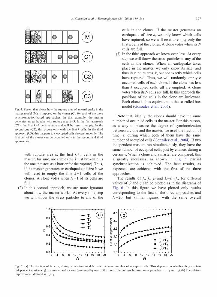
The exact rules for driving the clones will follow oneof the three approaches commented on below. Eachapproach imply a different knowledge of how the masterworks, and a different way of imposing the rupture areaon the clones. They are depicted in Fig. 4 and describedas follows:
(1) This first approach will indicate which is the bestresult that can be obtained with the synchroniza-tion-based forecasting. For this reason, the clonesare indeed minimalist models identical to themaster (González et al., 2004). The clones areloaded only if the master does not generate anearthquake in that time step. We know that in thiscase the particle in the master has gone to one ofthe cells i≥2, so the particles in the clones will berandomly thrown to the cells i≥2. We alsoconsider as known that, just after an earthquake
Fig. 4. Sketch that shows how the rupture area of an earthquake in themaster model (M) is imposed on the clones (C), for each of the threesynchronization-based approaches. In this example, the mastergenerates an earthquake with rupture area k=3. In the first approach(C1), the first k+1 cells rupture and will be reset to empty. In thesecond one (C2), this occurs only with the first k cells. In the thirdapproach (C3), this happens to k occupied cells chosen randomly. Thefirst cell of the clones can be occupied only in the second and thirdapproaches.
327Á. González et al. / Tectonophysics 424 (2006) 319–334
with rupture area k, the first k+1 cells in themaster, for sure, are stable (the k just broken plusthe one that acts as a barrier for the rupture). Thus,if the master generates an earthquake of size k, wewill reset to empty the first k+1 cells of theclones. A clone votes when N−1 of its cells arefull.
(2) In this second approach, we are more ignorantabout how the master works. At every time stepwe will throw the stress particles to any of the
Fig. 5. (a) The fraction of time, τ, during which two models have the samindependent masters (τ0) or a master and a clone (governed by one of the threimprovement, defined as τn /τ0.
cells in the clones. If the master generates anearthquake of size k, we only know which cellshave ruptured, so we will reset to empty only thefirst k cells of the clones. A clone votes when its Ncells are full.
(3) In the third approach we know even less. At everystep we will throw the stress particles to any of thecells in the clones. When an earthquake takesplace in the master, we only know its size, andthus its rupture area, k, but not exactly which cellshave ruptured. Thus, we will randomly empty koccupied cells of each clone. If the clone has lessthan k occupied cells, all are emptied. A clonevotes when its N cells are full. In this approach thepositions of the cells in the clone are irrelevant.Each clone is thus equivalent to the so-called boxmodel (González et al., 2005).
Note that, ideally, the clones should have the samenumber of occupied cells as the master. For this reason,as a way to measure the degree of synchronizationbetween a clone and the master, we used the fraction oftime, τ, during which both of them have the samenumber of occupied cells (González et al., 2004). If twoindependent masters run simultaneously, they have thesame number of occupied cells, just by chance, during acertain τ. When a clone and a master are compared, thisτ greatly increases, as shown in Fig. 5: partialsynchronization is achieved. The best results, asexpected, are achieved with the first of the threeapproaches.
The results of fa, fe, ff and L= fa+ fe, for differentvalues of Q and q can be plotted as in the diagrams ofFig. 6. In this figure we have plotted only resultscorresponding to the first of the three approaches andN=20, but similar figures, with the same overall
e number of occupied cells. This depends on whether they are twoe different synchronization approaches: τ1, τ2 and τ3). (b) The relative
Fig. 7. Loss function (L), fraction of alarm time ( fa), fraction of falsealarm time ( ff) and fraction of errors ( fe) obtained with the firstsynchronization-based forecasting approach, for N=20 and differentnumbers of clones (Q) along the rectilinear valley observed in L in Fig.6 (the first five points of each curve correspond to the cells marked inthat figure). The curves are exponential fits with three parameters.
Fig. 6. Fraction of alarm time ( fa), fraction of false alarm time (ff), fraction of errors ( fe), and loss function (L) obtained with the the firstsynchronization-based forecasting approach, for N=20 and different numbers of clones (Q) and votes (q). The squared cells mark a rectilinear valleyin the values of L.
328 Á. González et al. / Tectonophysics 424 (2006) 319–334
properties, can be drawn for the other two approachesand for any N (see below). There are simple trends inthese graphs. In Section 3 we noted that, in general, aforecasting strategy that produces lower fe tends toproduce higher fa and ff. If Q is fixed (same row), thegreater the q, the later the alarm is declared, so fa and ffare lesser and fe is greater. If q is fixed (same column),the greater the Q, the earlier the alarm is declared,resulting in the opposite trend.
We are interested in finding the combinations of Qand q that minimize L. The interesting fact is that the sumfa+ fe shows a rectilinear “valley” for certain combina-tions ofQ and q, marked with squares in the graph of Fig.6. This valley goes down as Q and q increase. In Fig. 7 itcan be observed that the valley goes down indefinitely,tending to a lowest asymptotic value of L. We estimatethis value, as a function of Q, with a three-parameterexponential fit of the form F=a exp[b / (Q+c)], where a,b, and c are parameters (Fig. 7). The value of a is theasymptotic one for Q→∞. This value is represented, foreach N, in Fig. 3. The fa, ff and fe also have asymptotictrends along this valley of L, also plotted in Fig. 7. Theycan also be fitted with the same kind of three-parameterdistribution, to estimate their asymptotic values as
Q→∞. A nice property is that, as shown in Fig. 7 for acertain case, these forecasting approaches predict mostof the characteristic earthquakes (fe is low), and have a
Fig. 9. Probability that a clone or thirty clones (with q=5; theuppermost squared cell in L in Fig. 6) declare an alarm in a given time,around the instant when it should for obtaining the ideal forecast.
329Á. González et al. / Tectonophysics 424 (2006) 319–334
very small fraction of false alarms. Note also that a fewtens of clones already render results close to theasymptotic ones.
As can be noted in Fig. 3, the synchronization-basedstrategies perform much better than a random guess, andalso much better than the reference strategy described inSection 4.2. Their results are intermediate between theideal forecast and the reference one. The second andthird synchronization-based approaches give onlyslightly greater L than the first one. The differencesare large only for small N. Although the first approachsynchronizes more efficiently each individual clonewith the master (Fig. 5), this effect is compensated byusing many clones.
To assess the performance of the method with largersystems, we plot in Fig. 8 the results of L for the threeapproaches, for N=100 and up to 60 clones. Asoccurred for smaller N, a rectilinear valley is observedin the graphs, and this tendency can be extrapolated toestimate the asymptotic value of L. Note that theresults for the first and second approaches are almostidentical (although L is slightly larger in the secondapproach). With the third approach, L decays to itsasymptotic value more slowly (the valley floor has asmaller slope, so more clones are needed to achieve agiven low L). The asymptotic values of L, however,are very similar in the three cases (0.298 for the firstand second approaches; 0.306 for the third one). Notethat these values are smaller than for N=20, asexpected from the trend observed in Fig. 3. The fa, feand ff show trends similar to the ones described forFigs. 6 and 7. The asymptotic fe is very low (0.062,0.075 and 0.071 for the first, second, and thirdapproach, respectively).
Another way to measure the synchronization of theclones with the master is drawn in Fig. 9 for N=20. Theideal strategy (Section 4.3 and Appendix), would be todeclare the alarm just when N−1 cells of the master are
Fig. 8. Loss function (L) obtained with the three synchronization-based forecvotes (q). The squared cells mark rectilinear valleys in the values of L.
full. The figure shows how a single clone declares thealarm around that moment, but a group of clones does amuch better job.
6. Discussion and conclusions
In this paper we have tried to provide some insightinto how to synchronize numerical models with seismicfaults, in order to better forecast large earthquakes inthem. The idea is that, although we can rarely measure thestress and strain in actual faults, we can estimate therupture area and co-seismic displacement of their earth-quakes. If we force a calibrated model to reproduce everyearthquake rupture of the fault it simulates, probably themodel will be synchronized with the fault. Then it couldbe used to forecast the future evolution of the fault,including future large earthquakes. This idea is notcompletely new: e.g. Ward (2000) forced a model toreproduce a large-earthquake rupture and run the modelforward to see what could happen in the future. Theresults of this paper expand on earlier ones (González etal., 2004), and are still only theoretical, but fully
asting approaches, for N=100 and different numbers of clones (Q) and
330 Á. González et al. / Tectonophysics 424 (2006) 319–334
quantitative. We demonstrate that it is possible to partiallysynchronize numerical fault models between themselves,and use this to forecast synthetic earthquakes.
One of the models, called the master, evolves freely.We consider it as an actual fault, from which we canknow the rupture area of its earthquakes, but not thestrain or stress at depth. Our goal is to forecast thelargest earthquakes it generates. In the synchronization-based forecasting, we use several other models, calledclones, similar to the master (calibrated to have thesame average recurrence interval of large earthquakesthat the master has). These clones are equivalent to themodels that can be devised to simulate a seismic fault.They are run simultaneously and independently to themaster and to each other. We force them to reproducethe series of earthquake ruptures of the master, and thismakes them partially synchronized with it. In simplewords, if the master does not generate an earthquake,we preclude any earthquake in the clones; if the masterdoes generate an earthquake, we impose the samerupture area on the clones. When several of the clonesare highly loaded (strained), we declare an alarm,because the master is probably also highly loaded, andthus probably a large earthquake is impending. Thisprocedure efficiently predicts most of the largestearthquakes of the master, with a relatively low fractionof total alarm time and few false alarms. These resultsare robust: they are almost the same when the exactrules for imposing the earthquake ruptures vary, and thisgood performance is observed along the whole range ofmodel sizes considered. This synchronization-basedforecasting outperforms other procedures based only onthe earthquake series of the model (Vázquez-Prada etal., 2003; González et al., 2004).
The master and the clones are stochastic (random), soeach individual clone is only partially synchronized withthe master. However, when several clones are in thesame state, then it is more likely that the master is also inthis state, so the group of clones makes a much betterforecasting job than only one clone does. If the cloneswere deterministic, as a general rule only one would beneeded; more clones would have identical evolutions ifrun with the same initial conditions.
The procedure developed here is a kind of ensembleforecasting, in which several models are run to obtain abetter picture of how a system will evolve. This conceptis used in atmospheric forecasting (Palmer et al., 2005):several models are run simultaneously, and theiraverage result has a larger forecasting ability than thatof an individual model (Houghton, 2002; Palmer etal., 2005). Each model in this approach hasslightly different initial conditions, to take into account
measurement errors and then to represent one possiblestate of the atmosphere, among various possibilities. Inour approach, each clone marks a possible state of themaster among a range of possible options. Severaldeterministic clones could also be used with differentinitial conditions.
Our procedure also shares some similarities withcertain earthquake forecasting algorithms (Kossobokovet al., 1999; Keilis-Borok and Soloviev, 2003), in whichseveral seismicity functions are evaluated in real-time.When several of these functions indicate that a largeearthquake is probable, an alarm is declared. In our ap-proach, the clones are performing a role similar to thesefunctions, monitoring what is happening in the master.
Our proposal is that a possible way to synchronizemore complex, calibrated models with real faults mightbe to force them to reproduce the past series ofearthquakes (with the same rupture area and/or co-seismic displacement). This would need to be tested inthe future. Also it will be possible to test whether thisprocedure works in the forecasting of synthetic earth-quakes in other models.
Forcing the models to reproduce only one largeobserved rupture (as in Ward, 2000) probably is notenough (this is certainly the case in our stochasticmodel). Complex and chaotic systems, such as thelithosphere, are very sensitive to initial conditions.Forcing the model to reproduce only one rupture is anecessary and laudable first step, but probably does notconstrain the initial conditions sufficiently. We proposethat every observed rupture, albeit small, should beconsidered. Small earthquakes are much more frequentthan large ones, thus providing much more data.Moreover, they provide insight into the mechanicalstate of the crust (Seeber and Armbruster, 2000) and intothe mechanics of earthquake rupture (Rubin, 2002).They may indicate the patch of the fault plane which isexperiencing higher stresses and is likely to rupture inthe next large shock (Schorlemmer and Wiemer, 2005).Finally, they are important in the transfer of stress withinthe lithosphere, and in earthquake triggering (Helm-stetter et al., 2005).
Acknowledgments
Á.G. thanks Robert Shcherbakov for helping him toview the model with new eyes. We benefited from thereviews by Kristy F. Tiampo and an anonymousreviewer. Part of the numerical simulations were donein the computer cluster of the Institute of Biocomputingand Physics of Complex Systems (BIFI), at theUniversity of Zaragoza. The Spanish Ministry of
331Á. González et al. / Tectonophysics 424 (2006) 319–334
Education and Science funded this research by means ofthe project FIS2005-06237, and the grant AP2002-1347held by Á.G.
Appendix A. Deduction of the ideal forecastingstrategy
In this appendix we will deduce the ideal strategyoutlined in Section 4.3. This strategy renders the lowest(best) value of L= fa+ fe achievable in the minimalistmodel.
For this reasoning we would consider every cycle ofthe model as composed of two independent andconsecutive stages. The first, that will be called theloading stage, starts just after the occurrence of acharacteristic earthquake. During this stage the totalnumber of occupied cells grows, but not in a monotonicway, because the particles may land in already occupiedcells (and then be dissipated), and also because of theoccurrence of non-characteristic earthquakes (Fig. 2).When N−1 cells (all but the first one) become occupied,this first stage ends and the second stage, that will becalled the hitting stage (or plateau in the occupation),starts. In this second stage, the system resides staticallyin the state of maximum occupancy (Fig. 2) until aparticle arrives at the first cell. Then, a characteristicevent occurs, all the cells are emptied, and a new cyclebegins. The hitting stage can be mathematically treatedas a form of Russian roulette.
Both the time spent by the system in the loadingstage, x, and in the hitting stage, y, are statisticallydistributed. The distribution of y, denoted by P2(y), isgeometric. Considering that, in each time step, theprobability of hitting the first cell is p=1 /N, and itscomplementary is q=1−1 /N, it follows that
P2ðyÞ ¼ 1N
1−1N
� �y−1
; ðA:1Þ
whose mean is
hyi ¼ N ; ðA:2Þand whose standard deviation is
r ¼ N
ffiffiffiffiffiffiffiffiffiffi1−
1N
r: ðA:3Þ
The time elapsed between consecutive characteristicevents has been denoted by n, which is statisticallydistributed according to the function PN(n) (Vázquez-Prada et al., 2002, 2003; Gómez and Pacheco, 2004).Because the variables x and y are independent, the mean
length of the cycles ⟨n⟩ is the sum of the mean lengths ofthe two stages:
hni ¼ hxi þ hyi: ðA:4ÞIt is clear that the best L would be obtained only if we
knew the state of occupation of the system and couldmark, for each cycle, the instant at which the stage ofloading concludes. Let us explore the result of Lobtained if we turn the alarm on at a given value y=y0within the second stage of all the cycles. With thisstrategy, the fraction of errors is given by
feðy0Þ ¼Xy0
1P2ðyÞ ðA:5Þ
and inserting Eq. (A.1) we obtain
feðy0Þ ¼ 1−qy0 : ðA:6ÞWith respect to the fraction of alarm, its form is
faðy0Þ ¼
Xly¼y0
ðy−y0ÞdP2ðyÞ
hxi þ hyi ; ðA:7Þ
and inserting Eq. (A.1), we get
faðy0Þ ¼ Nqy0
hxi þ N: ðA:8Þ
Note the important contribution of the first stage ofthe process in the denominator. Thus, the specific formof the loss function is
Lðy0Þ ¼ 1−qy0 þ Nqy0
hxi þ N: ðA:9Þ
It is noteworthy that in the absence of the first stage,i.e. in the hypothesis of a pure geometric distribution,the value of L would be 1, not dependent on the value ofy0. The minimum value of L in Eq. (A.9) as a function ofy0 is obtained for y0=0, i.e. just after the end of the firststage, when the N−1 upper cells of the system becomefull. And this minimum value is
Lmin ¼ Nhni : ðA:10Þ
This result constitutes a rigorous lower bound for theexpected accuracy of any forecasting strategy in theminimalist model. For this model, ⟨n⟩ increases rapidlyas N grows (Gómez and Pacheco, 2004). This impliesthat the minimum L, obtained with this optimalforecasting strategy, decreases as N increases, asshown by the curve labeled as “Ideal” in Fig. 3. Thatis to say, minimalist models with more cells are more
332 Á. González et al. / Tectonophysics 424 (2006) 319–334
predictable. This is consistent with the fact that the timeseries of characteristic earthquakes is more periodic forlarger N (Gómez and Pacheco, 2004).
References
Aki, K., 1984. Asperities, barriers, characteristic earthquakes andstrong motion prediction. Journal of Geophysical Research 89,5867–5872.
Baba, T., Cummins, P.R., 2005. Contiguous rupture areas of twoNankai Trough earthquakes revealed by high-resolution tsunamiwaveform inversion. Geophysical Research Letters 32, L08305.
Bak, P., Tang, C., 1989. Earthquakes as a self-organized criticalphenomenon. Journal of Geophysical Research 94, 15635–15637.
Ben-Zion, Y., 2001. Dynamic ruptures in recent models of earthquakefaults. Journal of the Mechanics and Physics of Solids 49,2209–2244.
Boness, N.L., Zoback, M.D., 2004. Stress-induced seismic velocityanisotropy and physical properties in the SAFOD Pilot Hole inParkfield, CA. Geophysical Research Letters 13, L15S17.
Bowman, D.D., Ouillon, G., Sammis, C.G., Sornette, A., Sornette, D.,1998. An observational test of the critical earthquake concept.Journal of Geophysical Research 103, 24359–24372.
Castellaro, S., Mulargia, F., 2001. A simple but effective cellularautomaton for earthquakes. Geophysical Journal International 144,609–624.
Dahmen, K., Ertaş, D., Ben-Zion, Y., 1998. Gutenberg–Richterand characteristic earthquake behavior in simple mean-fieldmodels of heterogeneous faults. Physical Review E 58,1494–1501.
Das, S., Aki, K., 1977. Fault plane with barriers: a versatile earthquakemodel. Journal of Geophysical Research 82, 5658–5670.
Dowrick, D.J., Rhoades, D.A., 2004. Relations between earthquakemagnitude and fault rupture dimensions: how regionally variableare they? Bulletin of the Seismological Society of America 94,776–788.
Drossel, B., Schwabl, F., 1992. Self-organized criticality in a forest-firemodel. Physica A 191, 47–50.
Fitzenz, D.D., Miller, S.A., 2004. New insights on stress rotations froma forward regional model of the San Andreas fault system near itsBig Bend in southern California. Journal of Geophysical Research109, B08404.
Goltz, C., 1997. Fractal and Chaotic Properties of Earthquakes.Springer-Verlag, Berlin, Germany, p. 178.
Gómez, J.B., Pacheco, A.F., 2004. The minimalist model ofcharacteristic earthquakes as a useful tool for description of therecurrence of large earthquakes. Bulletin of the SeismologicalSociety of America 94, 1960–1967.
González, Á., Vázquez-Prada, M., Gómez, J.B., Pacheco, A.F., 2004.Using synchronization to improve the forecasting of largerelaxations in a cellular-automaton model. Europhysics Letters68, 611–617.
González, Á., Gómez, J.B., Pacheco, A.F., 2005. The occupation of abox as a toy model for the seismic cycle of a fault. AmericanJournal of Physics 73, 946–952.
Grant, L.B., Gould, M.M., 2004. Assimilation of paleoseismic data forearthquake simulation. Pure and Applied Geophysics 161,2295–2306.
Gutenberg, B., Richter, C.F., 1944. Frequency of earthquakes inCalifornia. Bulletin of the Seismological Society of America 34,185–188.
Gutenberg, B., Richter, C.F., 1954. Seismicity of the Earth andAssociated Phenomena, 2nd edn. Princeton University Press,Princeton, New Jersey, USA, p. 310.
Hainzl, S., Zöller, G., 2001. The role of disorder and stressconcentration in nonconservative fault systems. Physica A 294,67–84.
Hainzl, S., Zöller, G., Kurths, J., 1999. Self-organized criticality modelfor earthquakes: quiescence, foreshocks and aftershocks. Interna-tional Journal of Bifurcation and Chaos 9, 2249–2255.
Hainzl, S., Zöller, G., Kurths, J., Zschau, J., 2000. Seismic quiescenceas an indicator for large earthquakes in a system of self-organizedcriticality. Geophysical Researh Letters 27, 597–600.
Hashimoto, M., 2001. Complexity in the recurrence of largeearthquakes in southwestern Japan: a simulation with an interact-ing fault system model. Earth, Planets and Space 53, 249–259.
Heimpel, M.H., 2003. Characteristic scales of earthquake rupture fromnumerical models. Nonlinear Processes in Geophysics 10,573–584.
Helmstetter, A., Kagan, Y.Y., Jackson, D.D., 2005. Importance ofsmall earthquakes for stress transfers and earthquake triggering.Journal of Geophysical, Research 110, B05S08.
Henley, C.L., 1993. Statics of a “self-organized” percolation model.Physical Review Letters 71, 2741–2744.
Hickman, S., Zoback, M., 2004. Stress orientations and magnitudes inthe SAFOD pilot hole. Geophysical Research Letters 31, L15S12.
Houghton, J., 2002. The Physics of Atmospheres. CambridgeUniversity Press, Cambridge, UK, p. 320.
Ikeda, R., Iio, Y., Omura, K., 2001. In situ stress measurements inNIED boreholes in and around the fault zone near the 1995Hyogoken Nanbu earthquake, Japan. The Island Arc 10, 252–260.
Ishimoto, M., Iida, K., 1939. Observations sur les séismesenregistrés par le microséismographe construit dernièrement(I). Bulletin of the Earthquake Research Institute, University ofTokyo 17, 443–478.
Kanamori, H., Brodsky, E.E., 2004. The physics of earthquakes.Reports on Progress in Physics 67, 1429–1496.
Kanamori, H., Stewart, G.S., 1978. Seismological aspects ofGuatemala earthquake on February 4, 1976. Journal ofGeophysical Research 83, 3427–3434.
Kato, N., Seno, T., 2003. Hypocenter depths of large interplateearthquakes and their relation to seismic coupling. Earth andPlanetary Science Letters 210, 53–63.
Keilis-Borok, V.I., 2002. Earthquake prediction: state-of-the-art andemerging possibilities. Annual Review of Earth and PlanetarySciences 30, 1–33.
Keilis-Borok, V.I., Soloviev, A.A. (Eds.), 2003. Nonlinear Dynamicsof the Lithosphere and Earthquake Prediction. Springer, Berlin,p. 337.
Kossobokov, V.G., Romashkova, L.L., Keilis-Borok, V.I., Healy, J.H., 1999. Testing earthquake prediction algorithms: statisticallysignificant advance prediction of the largest earthquakes in theCircum-Pacific, 1992–1997. Physics of the Earth and PlanetaryInteriors 111, 187–196.
Kuroki, H., Ito, H.M., Takayama, H., Yoshida, A., 2004. 3-Dsimulation of the occurrence of slow slip events in the Tokai
333Á. González et al. / Tectonophysics 424 (2006) 319–334
region with a rate- and state-dependent friction law. Bulletin of theSeismological Society of America 94, 2037–2050.
Lei, X., Kusunose, K., Satoh, T., Nishizawa, O., 2003. The hierarchicalrupture process of a fault: an experimental study. Physics of theEarth and Planetary Interiors 137, 213–228.
López-Ruiz, R., Vázquez-Prada, M., Gómez, J.B., Pacheco, A.F.,2004. A model of characteristic earthquakes and its implicationsfor regional seismicity. Terra Nova 16, 116–120.
Main, I., 1996. Statistical physics, seismogenesis, and seismic hazard.Reviews of Geophysics 34, 433–462.
Mason, I.B., 2003. Binary forecasts. In: Joliffe, I.T., Stephenson, D.B.(Eds.), Forecast Verification: A Practitioner's Guide in Atmo-spheric Science. Wiley, West Sussex, UK, pp. 37–76. Referencesin pp. 215–226.
Michael, A.J., 2005. Viscoelasticity, postseismic slip, fault interac-tions, and the recurrence of large earthquakes. Bulletin of theSeismological Society of America 95, 1594–1603.
Miller, S.A., Ben-Zion, Y., Burg, J.-P., 1999. A three-dimensionalfluid-controlled earthquake model: behavior and implications.Journal of Geophysical Research 104, 10621–10638.
Molchan, G.M., 1997. Earthquake prediction as a decision-makingproblem. Pure and Applied Geophysics 149, 233–247.
Moreno, Y., Gómez, J.B., Pacheco, A.F., 1999. Self organizedcriticality in a fiber-bundle-type model. Physica A 274, 400–409.
Newman, W.I., Turcotte, D.L., 2002. A simple model for theearthquake cycle combining self-organized complexity withcritical point behavior. Nonlinear Processes in Geophysics 9,453–461.
Okada, T., Matsuzawa, T., Hasegawa, A., 2003. Comparison of sourceareas of M4.8±0.1 repeating earthquakes off Kamaishi, NE Japan:are asperities persistent features? Earth and Planetary ScienceLetters 213, 361–374.
Olami, Z., Feder, H.J.S., Christensen, K., 1992. Self-organizedcriticality in a continuous, nonconservative cellular autom-aton modeling earthquakes. Physical Review Letters 68,1244–1247.
Palmer, T.N., Shutts, G.J., Hagedorn, R., Doblas-Reyes, F.J., Jung, T.,Leutbecher, M., 2005. Representing model uncertainty in weatherand climate prediction. Annual Review of Earth and PlanetarySciences 33, 163–193.
Pepke, S.L., Carlson, J.M., 1994. Predictability of self-organizingsystems. Physical Review E 50, 236–242.
Preston, E.F., Sá Martins, J.S., Rundle, J.B., Anghel, M., Klein, W.,2000. Models of earthquake faults with long-range stress transfer.Computing in Science and Engineering 2, 34–41.
Reasenberg, P.A., 1999. Foreshock occurrence rates before largeearthquakes worldwide. Pure and Applied Geophysics 155,355–379.
Reinecker, J., Heidbach, O., Tingay, M., Sperner, B., Müller, B., 2005.The release 2005 of the World Stress Map (available online atwww.world-stressmap. org).
Robinson, R., 2004. Potential earthquake triggering in a complex faultnetwork: the northern South Island, New Zealand. GeophysicalJournal International 159, 734–748.
Robinson, R., Benites, R., 2001. Upgrading a synthetic seismicitymodel for more realistic fault ruptures. Geophysical ResearchLetters 28, 1843–1846.
Rubin, A.M., 2002. Aftershocks of microearthquakes as probes of themechanics of rupture. Journal of Geophysical Research 107, 2142.
Rundle, J.B., Klein, W., 1993. Scaling and critical phenomena in acellular automaton slider-block model for earthquakes. Journal ofStatistical Physics 72, 405–413.
Rundle, P.B., Rundle, J.B., Tiampo, K.F., Sa Martins, J.S., McGinnis,S., Klein, W., 2001. Nonlinear network dynamics on earthquakefault systems. Physical Review Letters 87, 148501.
Rundle, J.B., Turcotte, D.L., Shcherbakov, R., Klein, W., Sammis, C.,2003. Statistical physics approach to understanding the multiscaledynamics of earthquake fault systems. Reviews of Geophysics 41,1019.
Rundle, J.B., Rundle, P.B., Donnellan, A., Fox, G., 2004. Gutenberg–Richter statistics in topologically realistic system-level earthquakestress-evolution simulations. Earth, Planets and Space 56,761–771.
Rundle, J.B., Rundle, P.B., Donnellan, A., Li, P., Klein, W.,Morein, G., Turcotte, D.L., Grant, L., 2006. Stress transfer inearthquakes, hazard estimation and ensemble forecasting:inferences from numerical simulations. Tectonophysics 413,109–125.
Scholz, C.H., 2002. The Mechanics of Earthquakes and Faulting,2nd edn. Cambridge University Press, Cambridge, UK, p. 496.
Scholz, C.H., Gupta, A., 2000. Fault interactions and seismic hazard.Journal of Geodynamics 29, 459–467.
Schorlemmer, D., Wiemer, S., 2005. Microseismicity data forecastrupture area. Nature 434, 1086.
Schwartz, D.P., Coppersmith, K.J., 1984. Fault behavior andcharacteristic earthquakes: examples from the Wasatch and SanAndreas fault zones. Journal of Geophysical Research 89,5681–5698.
Seeber, L., Armbruster, J.G., 2000. Earthquakes as beacons of stresschange. Nature 407, 69–72.
Sieh, K., 1996. The repetition of large-earthquake ruptures. Proceed-ings of the National Academy of Sciences of the United States ofAmerica 93, 3764–3771.
Soloviev, A., Ismail-Zadeh, A., 2003. Models of dynamics of block-and-fault systems. In: Keilis-Borok, V.I., Soloviev, A.A. (Eds.),Nonlinear Dynamics of the Lithosphere and EarthquakePrediction. Springer, Berlin, Germany, pp. 71–139. Referencesin pp. 311–332.
Steacy, S.J., McCloskey, J., 1999. Heterogeneity and the earthquakemagnitude–frequency distribution. Geophysical Research Letters26, 899–902.
Stirling, M.W., Wesnousky, S.G., Shimazaki, K., 1996. Fault tracecomplexity, cumulative slip, and the shape of the magnitude–frequency distribution for strike–slip faults: a global survey.Geophysical Journal International 124, 833–868.
Stirling, M., Rhoades, D., Berryman, K., 2002. Comparison ofearthquake scaling relations derived from data of the instrumentaland preinstrumental era. Bulletin of the Seismological Society ofAmerica 92, 812–830.
Tanioka, Y., Hirata, K., Hino, R., Kanazawa, T., 2004. Slipdistribution of the 2003 Tokachi-oki earthquake estimated fromtsunami waveform inversion. Earth, Planets and Space 56,373–376.
Tiampo, K.F., Rundle, J.B., McGinnis, S.A., Klein, W., 2002. Patterndynamics and forecast methods in seismically active regions. Pureand Applied Geophysics 159, 2429–2467.
Tsukahara, H., Ikeda, R., Yamamoto, K., 2001. In situ stressmeasurements in a borehole close to the Nojima Fault. The IslandArc 10, 261–265.
Turcotte, D.L., 1997. Fractals and Chaos in Geology and Geophysics,2nd edition. Cambridge University Press, Cambridge, UK, p. 412.
Vázquez-Prada, M., González, Á., Gómez, J.B., Pacheco, A.F., 2002.A minimalist model of characteristic earthquakes. NonlinearProcesses in Geophysics 9, 513–519.
334 Á. González et al. / Tectonophysics 424 (2006) 319–334
Vázquez-Prada, M., González, Á., Gómez, J.B., Pacheco, A.F., 2003.Forecasting characteristic earthquakes in a minimalist model.Nonlinear Processes in Geophysics 10, 565–571.
Ward, S.N., 2000. San Francisco Bay area earthquake simulations: astep toward a standard physical earthquake model. Bulletin of theSeismological Society of America 90, 370–386.
Wells, D.L., Coppersmith, K.J., 1994. New empirical relationshipsamong magnitude, rupture length, rupture width, rupture area, andsurface displacement. Bulletin of the Seismological Society ofAmerica 84, 974–1002.
Wesnousky, S.G., 1994. The Gutenberg–Richter or characteristicearthquake distribution, which is it? Bulletin of the SeismologicalSociety of America 84, 1940–1959.
Wesnousky, S.G., Scholz, C.H., Shimazaki, K., Matsuda, T., 1983.Earthquake frequency distribution and the mechanics of faulting.Journal of Geophysical Research 88, 9331–9340.
Wyss, M., Habermann, R.E., 1988. Precursory seismic quiescence.Pure and Applied Geophysics 126, 319–332.
Yabuki, T., Matsu'ura, M., 1992. Geodetic data inversion using abayesian information criterion for spatial-distribution of fault slip.Geophysical Journal International 109, 363–375.
Yagi, Y., Kikuchi, M., Yoshida, S., Sagiya, T., 1999. Comparison ofthe coseismic rupture with the aftershock distribution in theHyuga-nada earthquakes of 1996. Geophysical Research Letters26, 3161–3164.
Yamamoto, K., Yabe, Y., 2001. Stresses at sites close to the NojimaFault measured from core samples. The Island Arc 10, 266–281.
Yeats, R.S., Sieh, K., Allen, C.R., 1997. The Geology of Earthquakes.Oxford University Press, New York, USA, p. 568.
Youngs, R.R., Coppersmith, K.J., 1985. Implications of fault slip ratesand earthquake recurrence models to probabilistic seismic hazardestimates. Bulletin of the Seismological Society of America 75,939–964.
Zoback, M.L., 1992. 1st-order and 2nd-order patterns of stress in thelithosphere — The World Stress Map project. Journal ofGeophysical Research 97, 11703–11728.
Zöller, G., Holschneider, M., Ben-Zion, Y., 2005. The role ofheterogeneities as a tuning parameter of earthquakes dynamics.Pure and Applied Geophysics 162, 1027–1049.