A ”well-balanced” finite volume scheme for blood

flow simulation

O. Delestre∗,†, P.-Y. Lagree†

May 29, 2012

Abstract

We are interested in simulating blood flow in arteries with a one di-mensional model. Thanks to recent developments in the analysis of hy-perbolic system of conservation laws (in the Saint-Venant/ shallow waterequations context) we will perform a simple finite volume scheme. Wefocus on conservation properties of this scheme which were not previouslyconsidered. To emphasize the necessity of this scheme, we present how atoo simple numerical scheme may induce spurious flows when the basicstatic shape of the radius changes. On contrary, the proposed schemeis ”well-balanced”: it preserves equilibria of Q = 0. Then examples ofanalytical or linearized solutions with and without viscous damping arepresented to validate the calculations. The influence of abrupt change ofbasic radius is emphasized in the case of an aneurism.

Keywords blood flow simulation; well-balanced scheme; finite volume scheme;hydrostatic reconstruction; man at eternal rest; semi-analytical solutions; shal-low water

1 Introduction

As quoted by Xiu and Sherwin [86] the one dimensional system of equationsfor blood flow in arteries was written long time ago by Leonhard Euler in 1775.Of course, he noticed (see Parker [64]) that it was far too difficult to solve.Since then, the pulsatile wave flow has been understood and is explained inclassical books such as Lighthill [50] and Pedley [65]. More recently a huge lotof work has been done and a lot of methods of resolution have been proposedto handle this set of equations, among them [81], [88], [73], [62], [44] [42] [71],[86], [25], [83], [58], [27], [15], [1], [16], [84], [84, 55]... and we forgot a lot ofactors. Even if recent progress of fluid structure interaction in 3D have beenperformed (Gerbeau et. al. [24], Van de Vosse et. al. [79], among others), thoseadvances have not made the 1-D modelisation obsolete. On the contrary, it isneeded for validation, for physical comprehension, for boundary conditions, fast

∗Corresponding author: Delestre@unice.fr, presently at: Laboratoire de MathematiquesJ.A. Dieudonne (UMR CNRS 7351) – Polytech Nice-Sophia , Universite de Nice – SophiaAntipolis, Parc Valrose, 06108 Nice cedex 02, France†CNRS & UPMC Universite Paris 06, UMR 7190, 4 place Jussieu, Institut Jean Le Rond

d’Alembert, Boıte 162, F-75005 Paris, France

1

arX

iv:1

205.

6033

v1 [

mat

h.N

A]

28

May

201

2

or real time computations and it is always relevant for full complex networksof arteries ([88], [73], [69], [62, 63]) or veins ([28]) or in micro circulation in thebrain [67].

In most of the previous references it is solved thanks to the method of char-acteristics, to finite differences or finite volumes (that we will discuss and im-prove in this paper), or finite elements methods (Galerkin discontinuous). Eachmethod has its own advantages.

In the meanwhile, the set of shallow water equations (though younger, asthe equations have been written by Adhemar Barre de Saint-Venant in 1871[18]) have received a large audience as well. They are used for modelling theflow in rivers [31], [12] (and networks of rivers), in lakes, rain overland flow[20, 21], [75], in dams [77, 78] or the long waves in shallow water seas (tides inthe Channel for example [70], or for Tsunami modelling [23], [68]). It has beenobserved that Saint-Venant equations with source terms (which are the shape ofthe topography, and the viscous terms) present numerical difficulties for steadystates. The splitting introduced by the discretisation creates an extra unphysicalflow driven by the change of the topography. A configuration with no flow, forexample a lake, will not stay at rest: thus, the so called equilibrium of the ”lakeat rest” is not preserved. So new schemes, called ”well-balanced” have beenconstructed to preserve this equilibrium. Bermudez and Vazquez [6, 5] havemodified the Roe solver to preserve steady states. Other ways to adapt exact orapproximate Riemann solver to non-homogeneous case have been proposed byLeVeque [47] and Jin [37]. Following the idea of the pioneer work of Greenbergand LeRoux [32], [30] and [29] have proposed schemes based on the solutionof the Riemann problem associated with a larger system (a third equation onthe bottom topography variable is added). A central scheme approach hasbeen developped in [41]. In Perthame and Simeoni [66], the source terms areincluded in the kinetic formulation. In [3] and [8], a well-balanced hydrostaticreconstruction has been derived. It can be applied to any conservative finitevolume scheme approximating the homogeneous Saint-Venant system. In [82],[17], [8] and [52, 51] the friction source term is treated under a well-balancedway. More recently, in [45], the system of shallow water with topography isrewritten under a homogeneous form. This enables them to get Lax-Wendroffand MacCormack well-balanced schemes. With well-balanced methods, spuriouscurrent does not appear.

Thus we will follow those authors and construct by analogy a similar methodbut for flows in elastic tubes rather than for free surface flows. Even if for arteryflows the wave behaviour of the solution is very important (forced regime withlot of reflexions), we have in mind complex networks. In this case we willhave to deal from the arteries to the veins with eventually microcirculationin the brain. In the smaller and softer vessels, the 1D approximation is stillvalid, the pulsatile behaviour is less important, and there are lot of changes ofsections (across stenosis, aneurisms, valves). Those changes of sections have tobe treated numerically with great care, which has not been the case up to nowin the litterature.

So here, we will follow the authors of the Saint-Venant community and con-struct by analogy a similar method but for artery flow. At first we derive theequations written in conservative form, looking in the literature, we found thatit has been only written by [83] in a PhD thesis and by [15], [16] but not ex-ploited in the ”well-balanced” point of view. Mostly ([86], [55]), equations are

2

in fact written in a non-conservative form. With non-conservative schemes, wehave consistency defaults and shocks are not uniquely defined, see among others[36], [7] and [13]. Furthermore, the discharge Q is not conserved. Not a lot ofattention has been attached to this problem up to now. But this non conser-vation is a real problem if we consider networks with tubes with non uniformsection and ultimately quasi steady flow in small terminal vessels.

Hence after the introduction of the set of equations in section 2 and derivingwith this new point of view the conservative equations, we construct by analogythe numerical scheme both at first and second order in section 3. Then section4 is devoted to several test cases to validate the different parts of the equations.The most important case is the ”man at eternal rest” by analogy to the ”lakeat rest” which would not be preserved by non-conservative schemes. The aimof this paper is to use this property to construct efficient methods of resolution.

2 The 1D model

2.1 Derivation of the equations

We first derive the model equations, they are of course now classical, as alreadymentioned. Starting from unsteady incompressible axi-symmetrical Navier-Stokes equations, and doing a long wave approximation one obtains a first setof Reduced Navier-Stokes equations ([42], [43]). One has the longitudinal con-vective term, the longitudinal pressure gradient, and only the transverse viscousterm, the longitudinal being negligible. The pressure is constant across the crosssection and depends only of x the longitudinal variable. The incompressibilityis preserved.

Then, integrating over the section, one obtains two integrated equations(kind of Von Karman equation). The first one is obtained from incompressibilityand application of boundary condition and relates the variation of section to thevariations of flow. The second one is obtained from the momentum. The finalequations are not closed and one has to add some hypothesis on the shape ofthe velocity profile to obtain a closed system (some discussions of this are in[42]). We then obtain the following system with dimensions which is the 1-Dmodel of flow: ∂tA+ ∂xQ = 0

∂tQ+ ∂xQ2

A+A

ρ∂xp = −Cf

Q

A

, (1)

where A(x, t) is the cross-section area (A = πR2, where R is the radius of thevessel), Q(x, t) = A(x, t)u(x, t) is the flow rate or the discharge, u(x, t) themean flow velocity, and ρ the blood density (see figure 1). The first equation iswithout any approximation. An extra factor of value 4/3 may appear in frontof Q2/A if the chosen profile is a Poiseuille profile (with either large viscosityν or low frequency ω/(2π) so that α = R0

√ω/ν the Womersley number is

small). This comes from the fact that this term is in fact an approximation

of∫ R0

2πu(t, x, r)2rdr (this u(t, x, r) being the actual longitudinal velocity, not

to be confused with u(x, t) =∫ R0

2πu(t, x, r)rdr). The chosen unit value cor-responds to a flat profile. The viscous term has been modelised by a frictionproportional to Q/A (see [87] [42]): Cf = 8πν where ν is the blood viscosity.Again, a friction term written −8πνQ/A is an approximation of the effective

3

term which is νR∂u/∂r|R (with here again u(t, x, r) the real longitudinal ve-locity). This specific choice corresponds to a Poiseuille flow (small α), and istherefore non consistent with the coefficient in the convective term. This isnot a real problem, those coefficients are adjusted in the literature. Note thatin Saint-Venant community, the skin friction modelling involves a square of Q,reminiscent to the turbulent nature of river flow. This is seldom used in blood-flow. To conclude on the mechanical modelling we will take the form of Eq. 1for granted and we will no more discuss it.

Finally, one has to model the arterial wall, the pressure has to be linked withthe displacement of the vessel. A simple elastic linear term in the variation ofradius is taken:

p− p0 = k(R−R0) or as well p = p0 + k

√A−√A0√

π, (2)

A0(x) is the cross section at rest (A0 = πR20, where R0 is the radius of the

vessel which may be variable in the case of aneurism, stenosis or taper), and thestiffness k is taken as a constant. The external pressure p0 is supposed constantas well. Again, this relation which is here a simple elastic string model maybe enhanced. Non linear terms, non local (tension) terms and/or dissipativeunsteady terms may be introduced (viscoelasticity). We take here the mostsimple law, but we are aware of the possibilities of complexity.

Note that the derivation of those equations may be done with only 1D fluidmechanics arguments ([67] or [39]). One has to be very careful then to writeprecisely the action of the pressure on the lateral walls (for example Kundu [40]page 793 does a mistake in his text book). But, the real point of view to derivethe equations is the one explained at the beginning of this section and involvesthe Reduced Navier-Stokes equations ([42]).

We will now change a bit this form to write a real conservative form. Notethat authors ([71], [55]) write system (1) as

∂tU + ∂xF (U) = S(U),

they use the variables U = (A, u), so that they identify a kind of flux F (U) =(Au, u2/2+p/ρ) and a source term S(U) = −Cfu/A. But u is not a conservativequantity, Q is, as we will see next.

Of course, those Saint-Venant and blood flow equations are very similar tothe 1D Euler compressible equations that one can write in nozzles, or in acoustics(Lighthill [50]), in this case the density ρ is variable and linked to the pressureby the isentropic law p ∝ ργ . This relation is the counter part of the relation ofpressure which are in Saint-Venant and respectively in the artery: hydrostaticbalance p = ρgη (density, gravitational acceleration, level of the free surface)and respectively the elasticity response of the artery p = k(R−R0) (stiffness ofthe wall, current radius of the vessel, reference radius at rest).

4

h

z

u uRR0x x

Figure 1: 1D models: left the blood flow model (u is the mean velocity, R theradius, A = πR2 the instantaneous area, R0 the radius at rest, A0 = πR2

0 thearea with no flow), right the shallow water model (u is the mean velocity, h thewater column height, z the topography).

2.2 Conservative system

So, to write the conservative system, the second equation of (1) is rewritten anddeveloped. Thus we get the following system of conservation laws:

∂tA+ ∂xQ = 0

∂tQ+ ∂x

[Q2

A+

k

3ρ√πA3/2

]=

kA

2ρ√π√A0

∂xA0 − CfQ

A

, (3)

we can write (3) under a more compact form:

∂tU + ∂xF (U) = S(U), (4)

with a new definition of U , F (U) and S(U). We identify U the vector of theconservative variables, F (U) the flux

U =

(AQ

), F (U) =

QQ2

A+

k

3ρ√πA3/2

(5)

and the source term takes into account the initial shape of the vessel A0 andthe friction term:

S(U) =

0kA

ρ√π∂x√A0 − Cf

Q

A

. (6)

This system is strictly hyperbolic when A > 0 (which should be the case inarteries). Indeed, this means that we have

∂xF (U) =

0 1

k√A

2ρ√π− Q2

A2

2Q

A

.∂x

(AQ

)= J(U).∂xU,

where the Jacobian matrix J(U) has two real eigenvalues (which is the definitionof hyperbolicity)

λ1 =Q

A−√k√A

2ρ√π

= u− c and λ2 =Q

A+

√k√A

2ρ√π

= u+ c. (7)

We recognise c as the well-known Moens Korteweg wave propagation speed([65]):

c =

√k√A

2ρ√π.

5

The system (3) without friction i.e. with Cf = 0 admits special solutions whichare steady state solutions, that means that we have

∂tA = ∂tu = ∂tQ = 0. (8)

Thus the mass conservation equation gives the discharge conservation: ∂xQ(x, t) =0. The momentum conservation equation, under the steady state and frictionlesshypothesis reduces to

∂x

[Q0

2

2A2+ b√A− b

√A0

]= 0, (9)

with b = k/(ρ√π). So that system (3) integrates to the two constants: Q(x, t) = Q0

Q02

2A2+ b√A− b√A0 = Cst

. (10)

The first is a constant flux, the second is the Bernoulli constant.We have of course made analogy between (3) and the one-dimensional Saint-

Venant (or shallow water) system:∂th+ ∂xq = 0

∂tq + ∂x

(q2

h+gh2

2

)= −gh∂xz − c|q|

q

hβ, (11)

where h(x, t) is the water height, u(x, t) the mean flow velocity, q(x, t) =h(x, t)u(x, t) the flow rate and z(x, t) the topography of the bottom and c isthe friction coefficient. With β = 2 we recover Chezy’s or Darcy-Weisbach’s law(depending on the way c is written) and with β = 7/3, we get the Manning-Strickler’s friction law.

This system admits steady state frictionless solutions too:

∂th = ∂tu = ∂tq = 0. (12)

Thus we get the conservation of discharge and the Bernoulli’s relation q = q0q0

2

2gh2+ z + h = Cst

, (13)

which is the exact analogous of (10). In the literature we can find numericalschemes preserving steady states under the form (13), but they are complex tohandle (see [14], [60], [76] and [9]). Most of the time, more simple steady statesare considered

q = u = 0

∂x

(gh2

2

)+ gh∂xz = 0

, (14)

which correspond from a mechanical point of view to the modelling of a ”lakeat rest”. We have a balance called hydrostatic balance between the hydrostaticpressure and the gravitational acceleration down an inclined bottom z. Thesecond term of (14) reduces to

H = h+ z = Cst, (15)

6

where H is the water level. Since the work of [32], schemes preserving at least(14) are called well-balanced schemes. This allows to have an efficient treatmentof the source term. Thus, in practice, schemes preserving (14) give good resultseven in unsteady cases. The analogous of the ”lake at rest” for the system(3) without friction, can be called the ”man at eternal rest” or ”dead manequilibrium”, it writes Q = u = 0

∂x

(k

3ρ√πA3/2

)− kA

ρ√π∂x√A0 = 0

. (16)

In this case we have√A =

√A0. We will now use this property to construct

the schemes.

xi−1 xi−1/2 xi xi+1/2 x

∆x

tn+1

O

t

tn∆tn

xi+1

Figure 2: The time and space stencil.

3 The numerical method

In this section, we describe the scheme for system (1) at first and second order,with the space and time discretisation illustrated in Figure 2.

3.1 Convective step

For the homogeneous system i.e. system (4) without source term: S(U) = 0, afirst-order conservative finite volume scheme writes simply (see figure 2):

Un+1i − Uni

∆t+Fni+1/2 − Fni−1/2

∆x= 0, (17)

where Uni is an approximation of U

Uni '1

∆x

∫ xi+1/2

xi−1/2

U(x, tn)dx

n refers to time tn with tn+1− tn = ∆t and i to the cell Ci = (xi−1/2, xi+1/2) =(xi−1/2, xi−1/2+∆x). The two points numerical flux Fi+1/2 is an approximationof the flux function (5) at the cell interface i+ 1/2

Fi+1/2 = F(Ui, Ui+1). (18)

This flux function will be detailed in section 3.3.

7

3.2 Source term treatment

3.2.1 ”Topography” treatment

The source termkA

ρ√π∂x√A0 is the analogous of the topography source term

(−gh∂xz) in the shallow water system (11). Looking at (3), it might be treatedexplicitly which writes

Un+1i = Uni −

∆t

∆x

(Fni+1/2 − Fni−1/2

)+ ∆tS(Uni ) (19)

where the source is written simply by evaluating the derivative of A0:

S(Uni ) =

0kAni

2ρ√π√A0i

A0i+1/2 −A0i−1/2

∆x

,

with the definition

A0i+1/2 =A0i+1 +A0i

2.

We will illustrate the fault of this naive method in sections 4.4 and 4.5. Wewill prefer a well-balanced method inspired from the hydrostatic reconstruction(see [3] and [8]). As for the hydrostatic reconstruction we do not consider thefriction term and we are looking for a scheme which preserves steady states atrest (16), the second equation in (16) means that we have

√A−

√A0 = Cst, (20)

as for the hydrostatic reconstruction we will use locally this relation to performa reconstruction of the variable A. On each part of the interface, we have thefollowing reconstructed variables

√Ai+1/2L = max(

√Ai + min(∆

√A0i+1/2, 0), 0)

Ui+1/2L = (Ai+1/2L, Ai+1/2Lui)t√

Ai+1/2R = max(√Ai+1 −max(∆

√A0i+1/2, 0), 0)

Ui+1/2R = (Ai+1/2R, Ai+1/2Rui+1)t

, (21)

where ∆√A0i+1/2 =

√A0i+1 −

√A0i.

For consistency the scheme (17) has to be slightly modified under the form

Un+1i = Uni −

∆t

∆x(Fni+1/2L − Fni−1/2R), (22)

whereFni+1/2L = Fni+1/2 + Si+1/2L

Fni−1/2R = Fni−1/2 + Si−1/2R, (23)

with

Si+1/2L =

(0

P(Ani )− P(Ani+1/2L)

)Si−1/2R =

(0

P(Ani )− P(Ani−1/2R)

) (24)

8

and

P(A) =k

3ρ√πA3/2. (25)

The numerical flux Fni+1/2 is now calculated with the reconstructed variables

(21):Fni+1/2 = F(Uni+1/2L, U

ni+1/2R).

Having treated the term linked to the variation of radius we now turn to thefriction term.

3.2.2 Friction treatment

Concerning the friction treatment two methods are presented here, namely: asemi-implicit treatment ([26], [11], and [49]) which is classical in shallow watersimulations and the apparent topography method (see [8], [54, 53]) which is awell-balanced method.

Semi-implicit treatment We use (22) as a prediction without friction, i.e.:

U∗i = Uni −∆t

∆x(Fni+1/2L − Fni−1/2R) (26)

and a friction correction (via a semi-implicit treatment) is applied on the pre-dicted variables (U∗i ):

A∗i

(un+1i − u∗i

∆t

)= −Cfun+1

i , (27)

thus we get un+1i and we have An+1

i = A∗i . It preserves zero velocity.

Apparent topography The apparent topography method (see [8]) consistsin writing the second equation of the system under the following form

∂tQ+ ∂x

[Q2

A+

k

3ρ√πA3/2

]=

kA

ρ√π∂x

√A0app, (28)

with

∂x

√A0app = ∂x

(√A0 + b

),

where

∂xb = −ρ√πCfk

Q

A2.

The hydrostatic reconstruction (21) is performed with the corrected term√A0app.

3.3 Numerical flux

Several numerical fluxes might be used, some of them are defined in the follow-ing.

9

Rusanov flux Following [8], the Rusanov flux writes

F(UL, UR) =F (UL) + F (UR)

2− cUR − UL

2,

withc = sup

U=UL,UR

( supj∈{1,2}

|λj(U)|),

where λ1(U) and λ2(U) are the eigenvalues of the system.

HLL flux Following [8], the HLL flux (Harten, Lax and van Leer [35]) writes

F(UL, UR) =

F (UL) if 0 ≤ c1c2F (UL)− c1F (UR)

c2 − c1+

c1c2c2 − c1

(UR − UL) if c1 < 0 < c2

F (UR) if c2 ≤ 0

,

(29)with

c1 = infU=UL,UR

( infj∈{1,2}

λj(U)) and c2 = supU=UL,UR

( supj∈{1,2}

λj(U)),

where λ1(U) and λ2(U) are the eigenvalues of the system.

VFRoe-ncv flux Adapting the main line of [56] and [57], we get the followingVFRoe-ncv flux for system (3)

F(UL, UR) =

F (UL) if 0 < λ1(U)

F (U∗) if λ1(U) < 0 < λ2(U)

F (UR) if λ2(U) < 0

,

with the mean state

W =

(4cu

)=

(2 (cL + cR)uL + uR

2

)

and

U∗ =

(A∗A∗u∗

),

where A∗ et u∗ are the Roe mean states, we get them thanks the Riemanninvariant {

uR − 4cR = u∗ − 4c∗uL + 4cL = u∗ + 4c∗

, (30)

thus we have {u∗ = u− 2(cR − cL)

c∗ = c− 1

8(uR − uL)

.

When λ1(UL) < 0 < λ1(UR) or λ2(UL) < 0 < λ2(UR), we can get non entropicsolutions. We perform an entropy correction thanks to the Rusanov flux.

10

Kinetic flux Adapting the main line of [2] and [4], we get the following kineticflux for system (3)

F(UL, UR) = F+(UL) + F−(UR),

with

F+(UL) =AL

2√

3TL

M+2 −M−2

2M+

3 −M−3

3

F−(UR) =AR

2√

3TR

m+2 −m−2

2m+

3 −m−3

3

where

M+ = max(0, uL +√

3TL)M− = max(0, uL −

√3TL)

m+ = min(0, uR +√

3TR)m− = min(0, uR −

√3TR)

with

TL =k

3ρ√π

√AL and TR =

k

3ρ√π

√AR.

CFL condition We have to impose a CFL (Courant, Friedrichs, Levy) con-dition on the timestep to prevent blow up of the numerical values and to ensurethe positivity of A. This classical stability condition writes

∆t ≤ nCFLmini

(∆xi)

maxi

(|ui|+ ci),

where ci =√k√Ai/(2ρ

√π) and nCFL = 1 (resp. nCFL = 0.5) for the first

order scheme (resp. for the second order scheme see 3.5).We have to notice that the kinetic flux needs a particular CFL condition

(see [2, p.24])

∆t ≤ nCFLmini

(∆xi)

maxi

(|ui|+√

3Ti).

The Rusanov is the most diffusive but the most simple to implement, thekinetic one is slightly less diffusive but more cpu time consuming. VFRoe-ncvand HLL are comparable, but the first one is a little more time consuming dueto entropy correction. All these fluxes are compared in [19] in Saint-Venantframework.

3.4 Boundary conditions

3.4.1 Characteristic system

Of course boundary conditions are very important for artery flow. We willnot too much insist on them, and we will not present for example the classicalWindkessel model or variations. Nevertheless, adapting [11] to blood flow, we

11

can write the homogeneous form of (4) under the following non conservativeform

∂tA+ u∂xA+A∂xu = 0

∂tu+k

2ρ√π√A∂xA+ u∂xu = 0

. (31)

Thanks to the Moens Korteweg velocity rewritten as A = c4π(2ρ/k)2, we get{∂t [4c− u] + (u− c)∂x [4c− u] = 0∂t [4c+ u] + (u+ c)∂x [4c+ u] = 0

, (32)

thus we haved(4c− u)

dt= 0 (respectively

d(4c+ u)

dt= 0) or the Riemann in-

variant 4c − u = Cst (resp. 4c + u = Cst) along the characteristic curve C−

(resp. C+) defined by the equationdx

dt= u− c (resp.

dx

dt= u+ c).

The boundary conditions will be prescribed thanks to the method of char-acteristics. We set Ubound = U(0) or U(L) and Unear = U(∆x) or U(L −∆x)depending on the considered boundary (x = 0 or x = L).

3.4.2 Subcritical flow

We write here boundary condition for subcritical flow: at the boundary the flowis subcritical if we have |ubound| < cbound or equivalently

(ubound − cbound) (ubound + cbound) < 0. (33)

Of course it seems to be always the case in blood flows, where |Q/(Ac)| isless than 10 % in physicological cases. This concept is more relevant to Saint-Venant equation, where supercritical flow are easily obtained. Two cases arepossible: we are given either the cross section A (the pressure thanks to (2)) orthe discharge Q.

• Given cross section Abound = Cst:

At x = 0 the Riemann invariant is constant along the ingoing characteristicu− c, thus we have{

Abound = Cstubound = unear − 4 [cnear − cbound] . (34)

At x = L the Riemann invariant is constant along the outgoing charac-teristic u+ c, thus we have{

Abound = Cstubound = unear + 4 [cnear − cbound] . (35)

If (33) is not verified by the couple (Abound, ubound), the flow is in factsupercritical.

• Given discharge Qbound = Cst:

Depending on the boundary considered we have either at x = 0

0 = −Qbound + (unear − 4cnear)Abound + 4cboundAbound, (36)

12

or at x = L

0 = −Qbound + (unear + 4cnear)Abound − 4cboundAbound. (37)

We recall that cbound depends on Abound, we solve (36) or (37) to getAbound.

The source terms might be considered negligible in the characteristic method.

3.4.3 Supercritical flow

As previously mentioned, this is not really a relevant case for flows in arteries.But, in veins, or in collapsible tubes, it may be relevant (see Pedley [65]). Asupercritical inflow corresponds to both Abound = Cst1 and Qbound = Cst2 thathave to be imposed. A supercritical outflow is such that we have Abound = Anearand Qbound = Qnear.

Again, source terms are neglected in the characteristic method.In order to impose the discharge Qbound = Aboundubound, we can use an other

method: the use of the first component of the numerical flux is an accurate wayto proceed, even if F1(UL, UR) = Qbound(t) has no unique solution (and thecomplexity of the problem depends on the numerical flux).

3.5 Second order scheme

In order to get a second order scheme, we use the following algorithm:

Step 1 In order to get second order reconstructed variables(U•±,

√A0•±

)we

perform a linear reconstruction on variables u, A,√A − √A0 then we get the

reconstruction on√A0.

We consider the scalar function s ∈ R, its linear reconstruction is defined by

si−1/2+ = si −∆x

2Dsi and si+1/2− = si +

∆x

2Dsi

where D is one of the following reconstruction operator Dmuscl, Deno andDenom. To get the reconstruction operator D, we introduce the minmod slopelimiter

minmod(x, y) =

min(x, y) if x, y ≥ 0max(x, y) if x, y ≤ 00 else

.

Some other slope limiters might be found in [48, p.111-112] (the MonotonizedCentral difference limiter and the Superbee limiter).

MUSCL With the operator

Dmusclsi = minmod

(si − si−1

∆x,si+1 − si

∆x

),

we get the MUSCL linear reconstruction (Monotonic Upwind Scheme for Con-servation Law [80]). We can find a less diffusive but more complicated form ofthe MUSCL reconstruction in [22].

13

ENO With the operator

Denosi = minmod

(si − si−1

∆x+ θeno

∆x

2D2si−1/2,

si+1 − si∆x

+ θeno∆x

2D2si+1/2

),

where

D2si+1/2 = minmod

(si+1 − 2si + si−1

∆x2,si+2 − 2si+1 + si

∆x2

)and

θeno = 1,

we perform the ENO linear reconstruction (Essentially Non Oscillatory [34, 33],[72]). This reconstruction is more accurate than the MUSCL reconstruction butless stable. In order to get a more stable reconstruction we can take θeno in [0, 1](it is recommended to take θeno = 0.25 [10, p.236]).

modified ENO With the operator

Denomsi = minmod (Denosi, 2θenomDmusclsi) , with θenom ∈ [0, 1],

we get the modified ENO linear reconstruction [8, p.55-56] and [10, p.235-237].The previous linear reconstructions applied to A writes

Ai−1/2+ = Ai −∆x

2DAi, Ai+1/2− = Ai +

∆x

2DAi,

thus we have the following conservation relation

Ai−1/2+ +Ai+1/2−

2= Ai.

In order to get the same kind of relation on the discharges, the following modifiedreconstruction is performed on the velocity variables u

ui−1/2+ = ui −Ai+1/2−

Ai

∆x

2Dui, ui+1/2− = ui +

Ai−1/2+

Ai

∆x

2Dui,

this allows to get the conservation relation

Ai−1/2+ui−1/2+ +Ai+1/2−ui+1/2−

2= Aiui.

We perform on Ψ =√A−√A0 the same linear reconstruction as on A, we get

Ψ•± and at last we have√A0i+1/2± =

√Ai+1/2± −Ψi+1/2±.

Step 2 From variables U•− and U•+ we get the following reconstructed vari-ables

√Ai+1/2L = max(Ψi+1/2− + min(

√A0i+1/2−,

√A0i+1/2+), 0)

Ui+1/2L = (Ai+1/2L, Ai+1/2Lui+1/2−)t√Ai+1/2R = max(Ψi+1/2+ + min(

√A0i+1/2−,

√A0i+1/2+), 0)

Ui+1/2R = (Ai+1/2R, Ai+1/2Rui+1/2+)t

. (38)

14

Step 3 In order to get a consistent well-balanced scheme, it is necessary toadd a centered source term Fci. Scheme (17) becomes

Un+1i = Uni −

∆t

∆x

(Fni+1/2L − Fni−1/2R − Fcni

),

whereFni+1/2L = Fni+1/2 + Si+1/2−Fni−1/2R = Fni−1/2 + Si−1/2+

,

with

Si+1/2− =

(0

P(Ani+1/2−)− P(Ani+1/2L)

)Si−1/2+ =

(0

P(Ani−1/2+)− P(Ani−1/2R)

)and

Fci =

0

k

ρ√π

(Ani+1/2−)3/2 − (Ani−1/2+)3/2

3∆√A0i

,

with ∆√A0i =

√A0i+1/2−−

√A0i−1/2+. The numerical flux Fni+1/2 is calculated

as at first order (3.2.1), i.e. with the variables obtained with the hydrostaticreconstruction (38).

Thus we get a second order scheme in space which writes

Un+1 = Un + ∆tΦ(Un) with U = (Ui)i∈Z

and

Φ(Uni ) = − 1

∆x

(Fni+1/2L − Fni−1/2R − Fcni

). (39)

Step 4 The second order in time is recovered by a second order TVD (TotalVariation Diminishing) Runge-Kutta (see [72]), namely the Heun method

Un+1 = Un + ∆tΦ(Un),

Un+2 = Un+1 + ∆tΦ(Un+1),

Un+1 =Un + Un+2

2,

(40)

where Φ is defined by (39). This method is a kind of predictor-corrector method.A more complete modelling of the arterial flow will imply other source terms

(diffusion, tension,...). To observe those effects one has to use a higher orderscheme, as performed for shallow water in [59] and [57].

4 Validation

4.1 About the chosen examples

The chosen examples are more for sake of illustration of the previous schemerather than for validation on real clinical datas. So, the extremities of thearteries will be non reflecting and the numerical values are more indicative rather

15

than clinically relevant. Those examples will show that the scheme behaves welland that some validations from linearised or exact solutions may be reobtained.More specifically we insist on the cases with large change of initial section likesudden constriction and sudden expansion. Even we present here an aneurism,flow in a stenosis could also be treated.

4.2 The ideal tourniquet

In the Saint-Venant community, the dam break problem is a classical test case[74] (in compressible gas dynamics, it is referred as the Sod tube, LeVeque [46]or Lighthill [50] or [61]). We have an analytical solution of this problem thanksto the characteristic method. So, we consider the analogous of this problemin blood flow: a tourniquet is applied and we remove it instantaneously. Ofcourse, this is done in supposing that the pulsatile effects are neglected, so itis more a test case rather than a real tourniquet. Any way, with the previoushypothesis, we get a Riemann problem. This test allows us to study the abilityof the numerical scheme to give the front propagation properly, we notice thatthe non linear terms are tested (but neither the viscous ones nor the changeof basic radius). As we consider an artery with a constant radius at rest and

0.004

0.0042

0.0044

0.0046

0.0048

0.005

-0.04 -0.03 -0.02 -0.01 0 0.01 0.02 0.03 0.04

R (

m)

x (m)

t=0 s

(a)

RR

Rm

RL

-L/2 xA xB 0 xC L/2

R (

m)

x (m)

A

B C

t=1.5E-4 s

(b)

Figure 3: (a) The ideal tourniquet radius initial conditions: a discontinuousinitial radius (or pression) is imposed with no velocity (the blood is blocked),(b) analytical solution of the radius at time t > 0: a shock wave is movingdownstream (to the right) and an expansion wave upstream (to the left).

without friction, we consider the system (3) without source term. L is the lengthof the arteria with x ∈ [−L/2, L/2]. The initial conditions are

A(x, 0) =

{AL for x ≤ 0AR for x > 0

, (41)

with AL > AR and Q(x, 0) = u(x, 0) = 0 (see figure 3).As for the dam break, with the characteristic method we get an analytical

solution. At time t > 0, from the upstream to the downstream of the artery,we have four different states (as illustrated for the radius R =

√A/π in Figure

3b):

16

1. Upstream point A located at xA(t) = −cLt, the state is the same as theinitial one: {

A(x, t) = ALu(x, t) = 0

. (42)

2. Between point A and point B located at xB(t) = (uM − cM )t = (4cL −5cM )t (the subscript stands for the intermediate state in the followingzone), we have

u(x, t) =4

5

x

t+

4

5cL

c(x, t) = −1

5

x

t+

4

5cL

. (43)

3. Between point B and C located at xC(t) = st, with the Rankine Hugoniotrelation s = AMuM/(AM −AR). We have an intermediate state{

A(x, t) = AMu(x, t) = uM

, (44)

where the variables s, AM , uM and QM = uMAM are obtained thanks tothe following system

uM + 4cM = uL + 4cLQR −QM = s(AR −AM )(Q2R

AR+

k

3ρ√πAR

3/2

)−(Q2M

AM+

k

3ρ√πAM

3/2

)= s(QR −QM )

.

As uR = uL = QR = QL = 0, this system reduces touM + 4cM = 4cLQM = s(AM −AR)(Q2M

AM+

k

3ρ√πAM

3/2

)− k

3ρ√πAR

3/2 = sQM

.

This system is solved iteratively.

4. Downstream point C, the state is the same as the initial one{A(x, t) = ARu(x, t) = 0

. (45)

The simulations were performed with the first order scheme with each ofthe fluxes, J = 100 cells and a fix CFL of 1 (0.5 for the kinetic flux) andwe have used the following numerical values Cf = 0, k = 1.0 107Pa/m, ρ =1060m3, RL = 5. 10−3m, RR = 4. 10−3m, L = 0.08m, Tend = 0.005s, cR =√kRR/(2ρ) ' 4.34m/s, cL =

√kRL/(2ρ) ' 4.86m/s. An initial flow at rest:

Q(x, t = 0) = 0m3/s and

A(x, t = 0) =

{πRL

2, if x ∈ [−0, 04 : 0]πRR

2, if x ∈]0 : 0, 04].

As illustrated in Figure 4, we notice that the Rusanov and Kinetic fluxes aremore diffusive than the others. With mesh refinement and/or scheme order in-creasing, we should improve the results both at the shock level and the expansion

17

0.004

0.0042

0.0044

0.0046

0.0048

0.005

-0.04 -0.03 -0.02 -0.01 0 0.01 0.02 0.03 0.04

R (

m)

x (m)

Exact, t=0.005 sKinetic

RusanovVFRoe

HLL

(a)

0

1e-05

2e-05

3e-05

4e-05

5e-05

6e-05

7e-05

-0.04 -0.03 -0.02 -0.01 0 0.01 0.02 0.03 0.04

q (

m2/s

)

x (m)

Exact, t=0.005 sKinetic

RusanovVFRoe

HLL

(b)

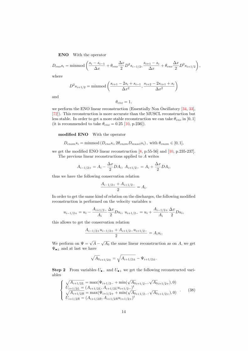
Figure 4: Snapshots of the ideal tourniquet – comparison between analyticaland numerical results at t = Tend: (a) radius and (b) discharge.

wave. As noticed in [19] for the shallow water equations, the VFRoe-ncv needsmore cpu time than the HLL flux. So in what follows we will focus on the HLLflux. This is a rather severe test case as in practice, |Q/(Ac)| is less than 10 %in physicological cases.

4.3 Wave equation

(a) (b)

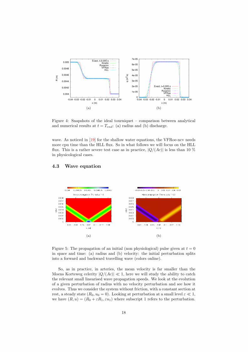
Figure 5: The propagation of an initial (non physiological) pulse given at t = 0in space and time: (a) radius and (b) velocity: the initial perturbation splitsinto a forward and backward travelling wave (colors online).

So, as in practice, in arteries, the mean velocity is far smaller than theMoens Korteweg celerity |Q/(Ac)| � 1, here we will study the ability to catchthe relevant small linearised wave propagation speeds. We look at the evolutionof a given perturbation of radius with no velocity perturbation and see how itevolves. Thus we consider the system without friction, with a constant section atrest, a steady state (R0, u0 = 0). Looking at perturbation at a small level ε� 1,we have (R, u) = (R0 + εR1, εu1) where subscript 1 refers to the perturbation.

18

Substitution in (3) and neglecting the small terms, it becomes the d’Alembertequation for the perturbations u1 and R1:

∂2t (u1, R1)− c02∂2x(u1, R1) = 0, (46)

the same is valid for variables Q1 = A0u1 the perturbation of flux and p1 = kR1

the perturbation of pressure with the Moens Korteweg wave velocity

c0 =

√k√A0

2ρ√π

=

√kR0

2ρ. (47)

With initial conditions u1(x, 0) = 0, R1(x, 0) = φ(x) we obtain so analyticalsolution: R(x, t) = R0 +

ε

2[φ (x− c0t) + φ (x+ c0t)]

u(x, t) = −ε2

c0R0

[−φ (x− c0t) + φ (x+ c0t)].

The following numerical values have been used for the figure 5: J = 200, Cf = 0,k = 1.0 108Pa/m, ρ = 1060m3, R0 = 4. 10−3m, L = 0.16m, Tend = 0.008s,c0 =

√kR0/(2ρ) ' 13.7m/s. As initial conditions, we take a fluid at rest

Q(x, 0) = 0m3/s with an initial deformation of the radius

A(x, 0) =

πR0

2, if x ∈ [0 : 40L/100] ∪ [60L/100 : L]

πR02

[1 + ε sin

(πx− 40L/100

20L/100

)]2, if x ∈]40L/100 : 60L/100[

,

with ε = 5.10−3. As illustrated, in Figure 6a, we get two waves, propagating onthe right (respectively left) with a positive (resp. negative) velocity. The twowaves are represented at several moments. We notice no numerical diffusion.

0.004

0.004005

0.00401

0.004015

0.00402

0.004025

0 0.02 0.04 0.06 0.08 0.1 0.12 0.14 0.16

R [m

]

x [m]

Exactt=0

t=Tend/4t=Tend/2

t=3Tend/4

(a)

-25

-24.5

-24

-23.5

-23

-22.5

-22

-21.5

-21

-20.5

4.5 5 5.5 6 6.5 7 7.5 8 8.5

log(|

|AJ-A

2J||

L1)

log(J)

Order 1y=-0.78x-17.03

Order 2y=-1.15x-15.42

(b)

Figure 6: (a) Radius as function of the position at 3 time steps: t = 0, t =Tend/4, t = Tend/2 and t = 3Tend/4, comparison between the first order schemewith HLL flux and exact solution and (b) the error made on the area calculationat t = 0.004s.

19

4.4 ”The man at eternal rest”

The previous test case did not involve drastic changes in the basic radius. Wewill show in this section that a not adapted source term treatment in (3) maygive non-physical velocity. In this test case, we consider a configuration withno flow and with a change of radius R0(x), this is the case for a dead man withan aneurism. Thus the section of the artery is not constant and the velocity isu(x, t) = 0 m/s. We use the following numerical values. J = 50 cells, Cf = 0,k = 1.0 108Pa/m, ρ = 1060m3, L = 0.14m, Tend = 5s. As initial conditions, wetake a fluid at rest Q(x, 0) = 0m3/s and

R(x, 0) = R0(x) =

Ro if x ∈ [0 : x1] ∪ [x4 : L]

Ro +∆R

2

[sin

((x− x1x2 − x1

π − π/2))

+ 1

], if x ∈]x1 : x2[

Ro + ∆R if x ∈ [x2 : x3]

Ro +∆R

2

(cos

(x− x3x4 − x3

π

)+ 1

), if x ∈]x3 : x4[

,

with Ro = 4.0 10−3m, ∆R = 1.0 10−3m, x1 = 1.0 10−2m, x2 = 3.05 10−2m,x3 = 4.95 10−2m and x4 = 7.0 10−2m (figure 7a).

As illustrated in Figure 7b, with an explicit treatment of the source term inA0, we get non zero velocities at the arteria cross section variation level. The”man at eternal rest” is not preserved, spurious flow appear (avoiding artifactssuch as [38]). As expected, the hydrostatic reconstruction (21) preserves exactlythe steady state at rest.

0.0038

0.004

0.0042

0.0044

0.0046

0.0048

0.005

0.0052

0.0054

0 0.02 0.04 0.06 0.08 0.1 0.12 0.14

R (

m)

x (m)

the radius R

(a)

-0.8

-0.6

-0.4

-0.2

0

0.2

0.4

0.6

0.8

0 0.02 0.04 0.06 0.08 0.1 0.12 0.14

u (

m/s

)

x (m)

explicit treatmenthydrostatic reconstruction

(b)

Figure 7: The ”dead man case”: (a) the radius of the arteria, (b) comparisonof the velocity at time t = 5s between an explicit treatment of the source termand the hydrostatic reconstruction. The spurious flow effect is clearly visible ifan inappropriate scheme is chosen.

4.5 Wave reflection-transmission in an aneurism

4.5.1 Analytical linear transmission

We observed that waves propagate fairly well in a straight tube, we now observethe reflexion and transmission trough a sudden change of section (from AL to

20

AR) in an elastic tube. The d’Alembert equation (46) admits harmonic wavesei(ωt−x/c0), so that a plane wave is (symbol 1 represents a linear perturbationas in section 4.3):

Q1 = Y0p1, with p1 ∝ Re(ei(ωt−x/c0))and Y0 = A0/(ρc0) is called the characteristic admittance. With this definition,we can look at a change of section from a radius RL to a radius RR: an imposedright traveling plane wave ei(ωt−x/cL) moving at celerity cL in the left media(subscript L) will experience a transmission in the right media (subscript R)(and will move at celerity cR) and a reflexion (and move at celerity −cL). Thecoefficients of transmission and reflexion depend on the two admittances of thetwo media L and R (see Lighthill or Pedley):

Tr =2YL

YL + YRand Re =

YL − YRYL + YR

.

As the admittance does not depend on the frenquency ω, any signal (by Fourierdecomposition) will be transmitted and reflected with those values.

Here we will study the reflection and the transmission of a small wave in ananeurism.

4.5.2 Propagation of a pulse to and from an expansion

(a) (b)

Figure 8: To an expansion, the propagation of an initial pulse in space and time:(a) radius and (b) velocity (colors online).

First we test the case of a pulse in a section RR passing trough an expansion:AL > AR, taking the following numerical values: J = 1500 cells, Cf = 0,k = 1.0 108Pa/m, ρ = 1060m3, RL = 5. 10−3m, RR = 4. 10−3m, ∆R =1.0 10−3m, L = 0.16m, Tend = 8.0 10−3s, cL =

√kRL/(2ρ) ' 15.36m/s and

cR =√kRR/(2ρ) ' 13.74m/s. We take a decreasing shape on a rather small

scale:

R0(x) =

RR + ∆R = Rb if x ∈ [0 : x1]

RR +∆R

2

[1 + cos

(x− x1x2 − x1

π

)]if x ∈]x1 : x2]

RR else

, (48)

21

-5e-06

0

5e-06

1e-05

1.5e-05

2e-05

0 0.02 0.04 0.06 0.08 0.1 0.12 0.14 0.16

R-R

0 [m

]

x [m]

εR0/2εR0Tr/2

εR0Re/2

t=0t=Tend/4

t=3Tend/4

Figure 9: Radius as function of the position at 3 time steps: t = 0, t = Tend/4,t = Tend/2 and t = 3Tend/4. The dotted lines represent the level of the predictedreflexion (Re) and transmission (Tr) coefficients.

with x1 = 19L/40 and x2 = L/2. As initial conditions, we consider a fluid atrest Q(x, 0) = 0m3/s and the following perturbation of radius:

R(x, 0) =

R0(x)

[1 + ε sin

(100

20Lπ

(x− 65L

100

))]if x ∈ [65L/100 : 85L/100]

R0(x) else,

with ε = 5.0 10−3.

(a) (b)

Figure 10: From an expansion, the propagation of an initial pulse in space andtime: (a) radius and (b) velocity (colors online).

Results showing the wave propagation and expansion are in Figure 8. InFigure 9 we have the amplitude of the pulse before and after the change ofsection, the level of the analytical prediction of T and R is plotted as wellshowing that the levels are preserved.

The same is done for a pulse propagating from an expansion. So, just the

22

-5e-06

0

5e-06

1e-05

1.5e-05

2e-05

2.5e-05

0 0.02 0.04 0.06 0.08 0.1 0.12 0.14 0.16

R-R

0 [m

]

x [m]

εR0/2εR0Tr/2

εR0Re/2

t=0t=T/4

t=3T/4

Figure 11: Radius as function of the position at 3 time steps: t = 0, t = Tend/4,t = Tend/2 and t = 3Tend/4. The dotted lines represent the level of the predictedreflexion (Re) and transmission (Tr) coefficients.

radius is changed:

R(x, 0) =

R0(x)

[1 + ε sin

(100

20Lπ

(x− 15L

100

))]if x ∈ [15L/100 : 35L/100]

R0(x) else,

with ε = 5.0 10−3. Similar results showing the wave propagation are in Figure10a and 10b. In Figure 11 the amplitude of the pulse corresponds to the levelpredicted by the analytical linearised solution.

4.5.3 The aneurism

(a) (b)

Figure 12: The propagation in an aneurysm of an initial pulse in space and time:(a) radius and (b) velocity. We note the expected reflexions at the position wherethe vessel changes his shape (colors online).

In this part we put an expansion and one constriction modelling an aneurism.An initial pulse at the center C of this aneurism propagates in the right and left

23

(a) (b)

Figure 13: A scheme which does not preserve the ”man at eternal rest” generatesspurious waves were the radius changes (colors online).

direction to the boundaries B. One sees in Figure 12 the reflexions and trans-missions at the position of the variation of radius. These plots have been donewith the following numerical values: J = 1500 cells, Cf = 0, k = 1.0 108Pa/m,ρ = 1060m3, RB = 4. 10−3m, RC = 5. 10−3m, ∆R = 1.0 10−3m, L = 0.16m,Tend = 8.0 10−3s, cB =

√kRB/(2ρ) ' 13.74m/s and cC =

√kRC/(2ρ) '

15.36m/s. With the given shape

R0(x) =

RB if x ∈ [0 : x1]⋃

[x4 : L]

RB +∆R

2

[1− cos

(x− x1x2 − x1

π

)]if x ∈]x1 : x2]

RB + ∆R = RC if x ∈]x2 : x3]

RB +∆R

2

[1 + cos

(x− x3x4 − x3

π

)]if x ∈]x3 : x4[

, (49)

with x1 = 9L/40, x2 = L/4, x3 = 3L/4 and x4 = 31L/40. As initial conditions,we consider a fluid at rest Q(x, 0) = 0m3/s and the initial perturbation:

R(x, 0) =

R0(x)

[1 + ε sin

(100

10Lπ

(x− 45L

100

))]if x ∈ [45L/100 : 55L/100]

R0(x) else,

with ε = 5.0 10−3.

4.5.4 Non adapted treatment of the source terms

To insist on the adapted treatment of the source terms, we present in this subsection what happens if a naive scheme is taken like in subsection 3.2.1. Weclearly see in Figure 13 that at the change of radius reflected and spuriouswave appear. The previous constant velocities are present like in Figure 13b.Furthermore, the initial data give traveling waves coming from the position ofthe change of section. This clearly shows the influence of the source terms inthe discretization.

24

4.6 Wave ”damping”

In this last test case, we look at the viscous damping term in the linearizedmomentum equation. This is the analogous of the Womersley [85] problem,we consider a periodic signal at the inflow which is a perturbation of a steadystate (R0 = Cst, u0 = 0) with a constant section at rest. We consider the setof equations 3 with the friction term under the nonconservative form with thevariables (R, u), this system writes

∂tR+ u∂xR+R

2∂xu = 0

∂tu+ u∂xu+k

ρ∂xR = −Cf

π

u

R2

.

We take R = R0 + εR1 and u = 0 + εu1, where (R1, u1) is the perturbation ofthe steady state. We have after linearisation of the equations: 2∂tR1 +R0∂xu1 = 0

∂tu1 +k

ρ∂xR1 = −Cf

π

u1

R02

,

which may be combined in two wave equations with source term

∂2t (u1, R1)− c02∂2x(u1, R1) = −Cfπ

∂t(u1, R1)

R02 . (50)

Looking for progressive waves (i.e. under the form ei(ωt−Kx)), we obtain thedispersion relation

K2 =ω2

c02− i ωCf

πR0c02, (51)

with ω = 2π/Tpulse, Tpulse the time length of a pulse and K = kr + iki, thewave vector not to be confused with the stiffness,

kr =

[ω4

c04+

(ωCf

πR02c02

)2]1/4

cos

(1

2arctan

(− Cf

πR02ω

))

ki =

[ω4

c04+

(ωCf

πR02c02

)2]1/4

sin

(1

2arctan

(− Cf

πR02ω

)) . (52)

For the numerical applications, we impose the incoming discharge

Qb(t) = Qamp sin(ωt)m3/s,

with Qamp the amplitude of the inflow discharge. We get a damping wave inthe domain

Q(t, x) =

{0 , if krx > ωtQamp sin (ωt− krx) ekix , if krx ≤ ωt , (53)

where Qb(t) is the discharge imposed at x = 0.The following numerical values allow to plot figure 14a to 14d. For Cf , we

took 4 different values (Cf = 0, Cf = 0.000022, Cf = 0.000202 and Cf =

25

Cf

=0.0

00022

HL

L1-S

IH

LL

1-A

TH

LL

MU

SC

L-S

IH

LL

EN

O-S

IH

LL

MU

SC

L-A

T

J||Q−

Qex|| L

1t c

pu

[s]||Q−

Qex|| L

1t c

pu

[s]||Q−

Qex|| L

1t c

pu

[s]||Q−

Qex|| L

1t c

pu

[s]||Q−

Qex|| L

1t c

pu

[s]

50

0.3

11E

-70.4

90.3

09E

-70.5

10.7

53E

-82.7

0.7

96E

-82.5

20.7

53E

-82.9

100

0.1

58E

-71.9

50.1

57E

-72

0.2

32E

-810.6

50.2

16E

-89.9

50.2

32E

-811.4

7

200

0.7

89E

-87.8

0.7

83E

-87.9

60.1

21E

-841.9

50.1

29E

-839.3

0.1

21E

-845.3

1

400

0.3

86E

-831.2

60.3

83E

-831.7

50.4

58E

-9167.1

60.6

51E

-9156.4

70.4

57E

-9179.4

800

0.1

83E

-8126.0

60.1

82E

-8126.9

20.2

67E

-9665.9

10.4

01E

-9625.6

20.2

67E

-9717.6

4

Reg

ress

ion

y=

-1.0

2x-1

3.2

7y=

-1.0

2x-1

3.2

7y=

-1.2

x-1

4.1

9y=

-1.0

4x-1

4.8

6y=

-1.2

x-1

4.1

9

Cf

=0.0

00202

HL

L1-S

IH

LL

1-A

TH

LL

MU

SC

L-S

IH

LL

EN

O-S

IH

LL

MU

SC

L-A

T

J||Q−

Qex|| L

1t c

pu

[s]||Q−

Qex|| L

1t c

pu

[s]||Q−

Qex|| L

1t c

pu

[s]||Q−

Qex|| L

1t c

pu

[s]||Q−

Qex|| L

1t c

pu

[s]

50

0.2

69E

-70.4

90.3

11E

-70.5

10.4

26E

-82.6

30.5

57E

-82.7

40.5

13E

-82.8

1

100

0.1

38E

-71.9

70.1

57E

-72

0.1

81E

-810.5

0.1

97E

-810.8

90.1

8E

-811.2

3

200

0.7

07E

-87.8

50.7

95E

-87.9

70.9

84E

-941.8

90.8

99E

-943.4

60.7

48E

-944.7

7

400

0.3

65E

-831.2

30.4

07E

-831.8

40.5

05E

-9167.1

80.4

99E

-9173.4

30.4

25E

-9180.5

2

800

0.1

92E

-8124.9

20.2

12E

-8127.3

10.2

83E

-9670.2

50.3

27E

-9694.6

90.2

96E

-9718.3

Reg

ress

ion

y=

-0.9

5x-1

3.7

y=

-0.9

7x-1

3.5

y=

-1.0

2x-1

5.2

4y=

-1.0

2x-1

5.2

y=

-1.0

3x-1

5.2

9

Cf

=0.0

05053

HL

L1-S

IH

LL

1-A

TH

LL

MU

SC

L-S

IH

LL

EN

O-S

IH

LL

MU

SC

L-A

T

J||Q−

Qex|| L

1t c

pu

[s]||Q−

Qex|| L

1t c

pu

[s]||Q−

Qex|| L

1t c

pu

[s]||Q−

Qex|| L

1t c

pu

[s]||Q−

Qex|| L

1t c

pu

[s]

50

0.2

6E

-70.5

10.3

96E

-70.5

20.1

62E

-72.6

80.1

59E

-72.7

90.3

34E

-72.8

1

100

0.1

46E

-71.9

80.2

15E

-72.0

30.9

16E

-810.5

60.8

99E

-811.0

30.1

76E

-711.2

200

0.7

9E

-87.8

80.1

12E

-78.0

10.4

94E

-841.9

40.4

86E

-843.7

10.9

07E

-844.6

9

400

0.4

11E

-831.3

20.5

76E

-831.9

0.2

57E

-8167.3

20.2

53E

-8174.2

50.4

6E

-8178.6

4

800

0.2

1E

-8125.1

50.2

91E

-8127.1

80.1

31E

-8669.5

60.1

29E

-8693.6

40.2

31E

-8714.2

9

Reg

ress

ion

y=

-0.9

1x-1

3.9

y=

-0.9

4x-1

3.3

3y=

-0.9

1x-1

4.3

4y=

-0.9

1x-1

4.3

6y=

-0.9

6x-1

3.4

3

Tab

le1:

Th

ew

ave

”dam

pin

g”:L1

erro

rson

the

dis

charg

eQ

an

dC

PU

tim

est cpu

forCf

=0.

000022,

0.000202

an

d0.0

05053.

(AT

)ap

par

ent

top

grap

hy,

(SI)

sem

i-im

pli

cit

and

(HL

L1)

firs

tord

ersc

hem

ew

ith

HL

Lfl

ux.

26

-3.5e-07

-3e-07

-2.5e-07

-2e-07

-1.5e-07

-1e-07

-5e-08

0

5e-08

0 0.5 1 1.5 2 2.5 3

Q [m

3/s

]

x [m]

Exact, Cf=0Rusanov1

HLL1Rusanov-MUSCL

HLL-MUSCLRusanov-ENO

HLL-ENO

(a)

-3.5e-07

-3e-07

-2.5e-07

-2e-07

-1.5e-07

-1e-07

-5e-08

0

5e-08

0 0.5 1 1.5 2 2.5 3

Q [m

3/s

]

x [m]

Exact, Cf=0.000022HLL1-SI

HLL1-ATHLL-MUSCL-SI

HLL-ENO-SIHLL-MUSCL-AT

(b)

-3e-07

-2.5e-07

-2e-07

-1.5e-07

-1e-07

-5e-08

0

5e-08

0 0.5 1 1.5 2 2.5 3

Q [m

3/s

]

x [m]

Exact, Cf=0.000202HLL1-SI

HLL1-ATHLL-MUSCL-SI

HLL-ENO-SIHLL-MUSCL-AT

(c)

-1.4e-07

-1.2e-07

-1e-07

-8e-08

-6e-08

-4e-08

-2e-08

0

2e-08

0 0.5 1 1.5 2 2.5 3

Q [m

3/s

]

x [m]

Exact, Cf=0.005053HLL1-SI

HLL1-ATHLL-MUSCL-SI

HLL-ENO-SIHLL-MUSCL-AT

(d)

Figure 14: The damping of a discharge wave (a) Cf = 0, α = ∞, (b) Cf =0.000022, α = 15.15, (c) Cf = 0.000202, α = 5 and (d) Cf = 0.005053, α = 1.The friction has been treated with either the semi-implicit method (SI) or theapparent topography method (AT) and J = 800.

27

0.005053, corresponding to Womersley parameters α = ∞, α = 15.15, α = 5and α = 1), J = 50, 100, 200, 400, 800 cells, k = 1.108Pa/m, ρ = 1060m3,R0 = 4.10−3m, L = 3m, Tend = 25.s. As initial conditions, we take a fluid atrest Q(x, 0) = 0m3/s and as input boundary condition

Qb(t) = Qamp sin(ωt)m3/s.

with ω = 2π/Tpulse = 2π/0.5s and Qamp = 3.45.10−7m3/s. As the flow issubcritical,the discharge is imposed at the outflow boundary thanks to (53)with x = L.

In this part, we insist on the comparison between first order and secondorder. So, we compare first order (HHL1) and second order scheme with bothMUSCL (HLL MUSCL) and ENO (HLL ENO) linear reconstruction. WhenCf is not null, semi-implicit (SI) and apparent topography (AT) are compared.We should remark that as the friction increases the structure of the system(1) changes and goes from a transport/ wave behavior to a diffusive behavior.The diffusive behavior comes from the fact that as Cf increases, finally themomentum equation contains at leading order only the friction term and theelastic one: CfQ1/A0 ∼ −(A0k/ρ)∂xR and so, using the conservation of mass:

∂R

∂t= D

∂2R

∂x2with D =

kπR20

2ρCf,

which is consistent with (51) at small ω. However solving a ”heat equation” witha ”wave technique” seems to be adapted. Indeed, we notice a fair agreementbetween the numerics and the analytical solution in Figures 14a to 14d. ”Errorsmade” between numerical results and the exact solution of the linearized systemare given for information with CPU time in tables 1 and 2.

4.7 Discussion on numerical precision

Indeed, the notion of scheme order fully depends on the regularity of the solu-tion. Moreover, calculating the error on the solution of the linearized systemdoes not provide information from a numerical point of view (sections 4.3 and4.6). Our purpose is not to verify the second order accuracy of the numeri-cal method (it has already been verified for the Shallow Water applications in[8, 4, 22]). But these errors computations allow us to verify that for these config-urations the nonlinear system has a linear behavior. And this linear behavior isperfectly captured by the scheme and the physical model. Precision is increasedby increasing the order of the numerical method (as shown on Figure 6b andas illustrated in tables 1 and 2). The theoretical order of the schemes is notrecovered for the wave test in section 4.3 (0.78 instead of 1 and 1.15 instead of2) this is due to the regularity of the solution of the initial system. Indeed, thissolution is only continuous. In addition, the system has no term of order 2, thenthe interest in using a second order method is to save computing time for a givenaccuracy (see Figure 15). The semi-implicit treatment and the apparent topog-raphy give closed results. However, when friction increases (Cf = 0.005053),the semi-implicit method is closer to the linearised solution.

28

-1

0

1

2

3

4

5

6

7

-22 -21.5 -21 -20.5 -20 -19.5 -19 -18.5 -18 -17.5 -17lo

g(t

cp

u)

log(||Q-Qex||L1)

HLL1-SIHLL1-AT

HLL-MUSCL-SIHLL-ENO-SI

HLL-MUSCL-AT

Figure 15: The wave ”damping”: The efficiency curves for Cf = 0.000202.

Cf = 0 HLL1 HLL MUSCL HLL ENO

J ||Q−Qex||L1 tcpu [s] ||Q−Qex||L1 tcpu [s] ||Q−Qex||L1 tcpu [s]

50 0.314E-7 0.49 0.104E-7 2.63 0.11E-7 2.7

100 0.159E-7 1.93 0.508E-8 10.49 0.546E-8 10.7

200 0.801E-8 7.7 0.238E-8 40.93 0.263E-8 42.6

400 0.397E-8 30.93 0.103E-8 163.47 0.118E-8 170.32

800 0.192E-8 123.28 0.36E-9 654.64 0.433E-9 681.26

Regression y=-1.007x-13.32 y=-1.2x-13.59 y=-1.155x-13.72

Table 2: The wave ”damping”: L1 errors on the discharge Q and CPU timestcpu for Cf = 0.

5 Conclusion

In this paper we have considered the classical 1-D model of flow in an artery,we have presented a new numerical scheme and some numerical tests. Thenew proposed scheme has been obtained in following recent advances in theshallow-water Saint-Venant community. This community has been confronted tospurious flows induced by the change of topography in not well written schemes.In blood-flows, it corresponds to the treatment of the terms due to a variatinginitial shape of the artery, which arises is stenosis, aneurisms, or taper. To writethe method, we have insisted on the fact that the effective conservative variablesare: the artery area A and the discharge Q, which was not clearly observed upto now. The obtained conservative system has been then discretized in order touse the property of equilibrium of ”the man at eternal rest” analogous to the”lake at rest” in Saint-Venant equations. If this property is not preserved inthe numerical stencil, spurious currents arise in the case of a variating vessel.For sake of illustration, if the terms are treated in a too simple way, we haveexhibited a case with an aneurism which induces a non zero flux of blood Q.In a pulsatile case, the same configuration creates extra waves as well. Ananalogous of dam break (here a tourniquet) was used to validate the other termsof the dicretisation. Other less demanding examples have been performed: linearwaves without and with damping in straight tubes. Good behaviour is obtainedin those pertinent test cases that explore all the parts of the equations.

The well-balanced finite volume scheme that we propose preserves the vol-

29

ume of blood and avoids non physical case behavior. Thus we get a stablescheme and the accuracy is improved thanks to a second order reconstruction.The numerical method has been tested on examples which are more ”gedanken”than physiological. This means that we only did a first necessary step. The nextone is now to test more complex cases such as bifurcations, special boundaryconditions and so on, in order to confront and fit to real practical clinical casesone of them being the case of aneurisms, in which as well we can introducea source term in the mass equation in the case of leaks, we conclude that tolook at those difficult problems, a careful treatment of the numerical scheme isimportant.

We thank ENDOCOM ANR for financial support, we thank Marie-OdileBristeau and Christophe Berthon for fruitful discussions.

References

[1] J. Alastruey, K. H. Parker, J. Peiro, and S. J. Sherwin. Lumped parameteroutflow models for 1-d blood flow simulations: Effect on pulse waves andparameter estimation. Commun. Comp. Phys., 4:317–336, 2008.

[2] E. Audusse. Schemas cinetiques pour le systeme de Saint-Venant. Master’sthesis, Universite Paris 6, 1999.

[3] E. Audusse, F. Bouchut, M.-O. Bristeau, R. Klein, and B. Perthame. Afast and stable well-balanced scheme with hydrostatic reconstruction forshallow water flows. SIAM J. Sci. Comput., 25(6):2050–2065, 2004.

[4] Emmanuel Audusse and Marie-Odile Bristeau. A well-balanced positivitypreserving ”second-order” scheme for shallow water flows on unstructuredmeshes. Journal of Computational Physics, 206:311–333, 2005.

[5] Alfredo Bermudez, Alain Dervieux, Jean-Antoine Desideri, and M. ElenaVazquez. Upwind schemes for the two-dimensional shallow water equa-tions with variable depth using unstructured meshes. Computer Methodsin Applied Mechanics and Engineering, 155(1-2):49 – 72, 1998.

[6] Alfredo Bermudez and M. Elena Vazquez. Upwind methods for hyperbolicconservation laws with source terms. Computers & Fluids, 23(8):1049 –1071, 1994.

[7] Christophe Berthon and Frederic Coquel. Nonlinear projection methodsfor multi-entropies navier-stokes systems. Mathematics of Computation,76:1163–1194, 2007.

[8] Francois Bouchut. Nonlinear stability of finite volume methods for hy-perbolic conservation laws, and well-balanced schemes for sources, volume2/2004. Birkhauser Basel, 2004.

[9] Francois Bouchut and Tomas Morales. A subsonic-well-balanced reconstruction scheme for shallow water flows.http://www.math.ntnu.no/conservation/2009/032.html, 2009. Preprint.

30

[10] Francois Bouchut, Haythem Ounaissa, and Benoıt Perthame. Upwindingof the source term at interfaces for euler equations with high friction. Com-puters and Mathematics with Applications, 53:361––375, 2007.

[11] Marie-Odile Bristeau and Benoıt Coussin. Boundary conditions for theshallow water equations solved by kinetic schemes. Technical Report 4282,INRIA, October 2001.

[12] J. Burguete, P. Garcıa-Navarro, and J. Murillo. Friction term discretizationand limitation to preserve stability and conservation in the 1d shallow-watermodel: Application to unsteady irrigation and river flow. InternationalJournal for Numerical Methods in Fluids, 58(4):403–425, 2008.

[13] Manuel J. Castro, Philippe G. LeFloch, Marıa Luz Munoz Ruiz, and CarlosPares. Why many theories of shock waves are necessary: Convergence errorin formally path-consistent schemes. Journal of Computational Physics,227(17):8107–8129, 2008.

[14] Manuel J. Castro, Alberto Pardo Milanes, and Carlos Pares. Well-balancednumerical schemes based on a generalized hydrostatic reconstruction tech-nique. Mathematical Models and Methods in Applied Sciences, 17(12):2065–2113, 2007.

[15] N. Cavallini, V. Caleffi, and V. Coscia. Finite volume and weno scheme inone-dimensional vascular system modelling. Computers and Mathematicswith Applications, 56:2382–2397, 2008.

[16] Nicola Cavallini and Vincenzo Coscia. One-dimensional modelling of venouspathologies: Finite volume and weno schemes. In Rolf Rannacher andAdelia Sequeira, editors, Advances in Mathematical Fluid Mechanics, pages147–170. Springer Berlin Heidelberg, 2010.

[17] Ashwin Chinnayya and A.-Y. LeRoux. A new General RiemannSolver for the Shallow Water equations, with friction and topography.http://www.math.ntnu.no/conservation/1999/021.html, 1999. Preprint.

[18] Adhemar Jean-Claude de Saint Venant. Theorie du mouvement non-permanent des eaux, avec application aux crues des rivieres et al’introduction des marees dans leur lit. Comptes Rendus de l’Academiedes Sciences, 73:147–154, 1871.

[19] Olivier Delestre. Simulation du ruissellement d’eau de pluie sur des surfacesagricoles/ rain water overland flow on agricultural fields simulation. PhDthesis, Universite d’Orleans (in French), available from TEL: tel.archives-ouvertes.fr/INSMI/tel-00531377/fr, July 2010.

[20] Olivier Delestre, Stephane Cordier, Francois James, and Frederic Darboux.Simulation of rain-water overland-flow. In Proceedings of the 12th Interna-tional Conference on Hyperbolic Problems, University of Maryland, CollegePark (USA), 2008, E. Tadmor, J.-G. Liu and A. Tzavaras Eds., Proceed-ings of Symposia in Applied Mathematics 67, Amer. Math. Soc., 537–546,2009.

31

[21] Olivier Delestre and Francois James. Simulation of rainfall events andoverland flow. In Proceedings of X International Conference Zaragoza-Pau on Applied Mathematics and Statistics, Jaca, Spain, september 2008,Monografıas Matematicas Garcıa de Galdeano, 2009.

[22] Olivier Delestre and Fabien Marche. A numerical scheme for a viscousshallow water model with friction. J. Sci. Comput., DOI 10.1007/s10915-010-9393-y, 2010.

[23] Denys Dutykh. Modelisation mathematique des tsunamis. PhD thesis, Ecolenormale superieure de Cachan, 2007.

[24] M. A. Fernandez, J.-F. Gerbeau, and C. Grandmont. A projection semi-implicit scheme for the coupling of an elastic structure with an incompress-ible fluid. International Journal for Numerical Methods in Engineering,69(4):794–821, 2007.

[25] Miguel Angel Fernandez, Vuk Milisic, and Alfio Quarteroni. Analysis of ageometrical multiscale blood flow model based on the coupling of ode’s andhyperbolic pde’s. Technical Report 5127, INRIA, February 2004.

[26] R. F. Fiedler and J. A. Ramirez. A numerical method for simulating dis-continuous shallow flow over an infiltrating surface. International Journalfor Numerical Methods in Fluids, 32:219–240, 2000.

[27] Luca Formaggia, Daniele Lamponi, Massimiliano Tuveri, and AlessandroVeneziani. Numerical modeling of 1d arterial networks coupled with alumped parameters description of the heart. Computer Methods in Biome-chanics and Biomedical Engineering, 9:273–288, 2006.

[28] Jose-Maria Fullana and Stephane Zaleski. A branched one-dimensionalmodel of vessel networks. J. Fluid. Mech., 621:183–204, 2009.

[29] T. Gallouet, J.-M. Herard, and N. Seguin. Some approximate godunovschemes to compute shallow-water equations with topography. Computers& Fluids, 32:479–513, 2003.

[30] L. Gosse. A well-balanced flux-vector splitting scheme designed for hy-perbolic systems of conservation laws with source terms. Computers &Mathematics with Applications, 39(9-10):135 – 159, 2000.

[31] N. Goutal and F. Maurel. A finite volume solver for 1D shallow-waterequations applied to an actual river. International Journal for NumericalMethods in Fluids, 38:1–19, 2002.

[32] J. M. Greenberg and A.-Y. LeRoux. A well-balanced scheme for the nu-merical processing of source terms in hyperbolic equation. SIAM Journalon Numerical Analysis, 33:1–16, 1996.

[33] Ami Harten, Bjorn Engquist, Stanley Osher, and Sukumar R.Chakravarthy. Uniformly High Order Accurate Essentially Non-oscillatorySchemes, III. Journal of Computational Physics, 71:231–303, August 1987.

32

[34] Ami Harten, Stanley Osher, Bjorn Engquist, and Sukumar R.Chakravarthy. Some results on uniformly high-order accurate essentiallynonoscillatory schemes. Applied Numerical Mathematics, 2(3-5):347 – 377,1986. Special Issue in Honor of Milt Rose’s Sixtieth Birthday.

[35] Amiram Harten, Peter D. Lax, and Bram van Leer. On upstream differ-encing and godunov-type schemes for hyperbolic conservation laws. SIAMReview, 25(1):35–61, January 1983.

[36] Thomas Y. Hou and Philippe G. LeFloch. Why nonconservative schemesconverge to wrong solutions: error analysis. Mathematics of Computation,62(206):497–530, April 1994.

[37] Shi Jin. A steady-state capturing method for hyperbolic systems withgeometrical source terms. M2AN, 35(4):631–645, July 2001.

[38] Robert Kirkman, Tony Moore, and Charlie Adlard. The Walking Dead.Image Comics, 2003.

[39] Pijush K. Kundu and Ira M. Cohen. Fluid Mechanics, Third Edition. 2004.

[40] Pijush K. Kundu and Ira M. Cohen. Fluid Mechanics, Fourth Edition.2008.

[41] Alexander Kurganov and Doron Levy. Central-upwind schemes for thesaint-venant system. Mathematical Modelling and Numerical Analysis,36:397–425, 2002.

[42] Pierre-Yves Lagree. An inverse technique to deduce the elasticity of a largeartery. The European Physical Journal, 9:153–163, 2000.

[43] Pierre-Yves Lagree and Sylvie Lorthois. The rns/prandtl equations andtheir link with other asymptotic descriptions. application to the computa-tion of the maximum value of the wall shear stress in a pipe. Int. J. Eng.Sci., 43/3–4:352–378, 2005.

[44] Pierre-Yves Lagree and Maurice Rossi. Etude de l’ecoulement du sang dansles arteres: effets nonlineaires et dissipatifs. C. R. Acad. Sci. Paris, t322,Serie II b, pages 401–408, 1996.

[45] Sang-Heon Lee and Nigel G. Wright. Simple and efficient solution of theshallow water equations with source terms. International Journal for Nu-merical Methods in Fluids, 63:313–340, 2010.

[46] Randall J. LeVeque. Numerical methods for conservation laws. Lectures inmathematics ETH Zurich. 1992.

[47] Randall J. LeVeque. Balancing source terms and flux gradients in high-resolution godunov methods: The quasi-steady wave-propagation algo-rithm. Journal of Computational Physics, 146(1):346 – 365, 1998.

[48] Randall J. LeVeque. Finite volume methods for hyperbolic problems. Cam-bridge Texts in Applied Mathematics. Cambridge University Press, Cam-bridge, 2002.

33

[49] Qiuhua Liang and Fabien Marche. Numerical resolution of well-balancedshallow water equations with complex source terms. Advances in WaterResources, 32(6):873 – 884, 2009.

[50] James Lighthill. Waves in Fluids. 1978.

[51] M. Lukacova-Medvid’ova and U. Teschke. Comparison study of some finitevolume and finite element methods for the shallow water equations withbottom topography and friction terms. J. Appl. Mech. Math. (ZAMM),86(11):874–891, 2006.

[52] M. Lukacova-Medvid’ova and Z. Vlk. Well-balanced finite volume evolutionGalerkin methods for the shallow water equations with source terms. In-ternational Journal for Numerical Methods in Fluids, 47(10-11):1165–1171,2005.

[53] A. Mangeney, F. Bouchut, N. Thomas, J. P. Vilotte, and M.-O. Bristeau.Numerical modeling of self-channeling granular flow and of their levee-channel deposits. Journal of Geophysical Research, 112(F2):F02017, May2007.

[54] A. Mangeney-Castelnau, F. Bouchut, J. P. Vilotte, E. Lajeunesse,A. Aubertin, and M. Pirulli. On the use of saint-venant equations to sim-ulate the spreading of a granular mass. Journal of Geophysical Research,110:B09103, 2005.

[55] Emilie Marchandise, Nicolas Chevaugeon, and Jean-Francois Remacle. Spa-tial and spectral superconvergence of discontinuous galerkin method forhyperbolic problems. Journal of Computational and Applied Mathematics,215(2):484–494, 2008. Proceedings of the Third International Conferenceon Advanced Computational Methods in Engineering (ACOMEN 2005).,Proceedings of the Third International Conference on Advanced Computa-tional Methods in Engineering (ACOMEN 2005).

[56] F. Marche, P. Bonneton, P. Fabrie, and N. Seguin. Evaluation of well-balanced bore-capturing schemes for 2D wetting and drying processes. In-ternational Journal for Numerical Methods in Fluids, 53:867–894, 2007.

[57] Fabien Marche and Christophe Berthon. A positive preserving high ordervfroe scheme for shallow water equations: A class of relaxation schemes.SIAM Journal on Scientific Computing, 30(5):pp. 2587–2612, August 2008.75M12, 35L65, 65M12.

[58] Vincent Martin, Francois Clement, Astrid Decoene, and Jean-Frederic Ger-beau. Parameter identification for a one-dimensional blood flow model. InEric Cances & Jean-Frederic Gerbeau, editor, ESAIM: PROCEEDINGS,volume 14, pages 174–200, September 2005.

[59] Sebastian Noelle, Normann Pankratz, Gabriella Puppo, and Jostein R.Natvig. Well-balanced finite volume schemes of arbitrary order of accuracyfor shallow water flows. Journal of Computational Physics, 213(2):474 –499, 2006.

34

[60] Sebastian Noelle, Yulong Xing, and Chi Wang Shu. High-order well-balanced finite volume weno schemes for shallow water equation with mov-ing water. Journal of Computational Physics, 226(1):29 – 58, 2007.

[61] Hilary Ockendon and Alan B. Tayler. Inviscid Fluid Flows. 1983.

[62] Mette S. Olufsen. Structured tree outflow condition for blood flow in largersystemic arteries. American Journal of Physiology – Heart and CirculatoryPhysiology, 276:257–268, 1999.

[63] Mette S. Olufsen, Charles S. Peskin, Won Yong Kim, Erik M. Pedersen,Ali Nadim, and Jesper Larsen. Numerical simulation and experimentalvalidation of blood flow in arteries with structured-tree outflow conditions.Annals of Biomedical Engineering, 28:1281–1299, 2000.

[64] Kim H. Parker. A brief history of arterial wave mechanics. Med Biol EngComput, 47:111–118, February 2009.

[65] T. J. Pedley. The Fluid Mechanics of Large Blood Vessel. 1980.

[66] B. Perthame and C. Simeoni. A kinetic scheme for the Saint-Venant systemwith a source term. Calcolo, 38:201–231, 2001. 10.1007/s10092-001-8181-3.

[67] Maciej Z. Pindera, Hui Ding, Mahesh M. Athavale, and Zhijian Chen. Ac-curacy of 1d microvascular flow models in the limit of low reynolds numbers.Microvascular Research, 77(3):273–280, 2009.

[68] Stephane Popinet. Quadtree-adaptative tsunami modelling. Ocean Dy-namics, pages 1–25, May 2011.

[69] Masashi Saito, Yuki Ikenaga, Mami Matsukawa, Yoshiaki Watanabe,Takaaki Asada, and Pierre-Yves Lagree. One-dimensional model for prop-agation of a pressure wave in a model of the human arterial network: Com-parison of theoretical and experimental. Journal of Biomechanical Engi-neering, 133, December 2011.

[70] Joe Sampson, Alan Easton, and Manmohan Singh. Modelling the effect ofproposed channel deepening on the tides in Port Phillip Bay. 2005.

[71] S. J. Sherwin, L. Formaggia, J. Peiro, and V. Franke. Computationalmodelling of 1d blood flow with variable mechanical properties and itsapplication to the simulation of wave propagation in the human arterialsystem. International Journal for Numerical Methods in Fluids, 43:673–700, 2003.

[72] C.-W. Shu and Stanley Osher. Efficient implementation of essentially non-oscillatory shock-capturing schemes. Journal of Computational Physics,77(2):439 – 471, 1988.

[73] N. Stergiopulos, D. F. Young, and T. R. Rogge. Computer simulation ofarterial flow with applications to arterial and aortic stenoses. J. Biome-chanics, 25(12):1477–1488, 1992.

[74] J. J. Stoker. Water Waves: The Mathematical Theory with Applications.Interscience Publishers, New York, USA, 1957.

35

[75] L. Tatard, O. Planchon, J. Wainwright, G. Nord, D. Favis-Mortlock, N. Sil-vera, O. Ribolzi, M. Esteves, and Chi-Hua Huang. Measurement and mod-elling of high-resolution flow-velocity data under simulated rainfall on alow-slope sandy soil. Journal of Hydrology, 348(1-2):1–12, January 2008.

[76] M. D. Thanh, Md. Fazlul Karim, and A. I. Md. Ismail. Well-balancedscheme for shallow water equations with arbitrary topography. Int. J.Dynamical Systems and Differential Equations, 1(3):196–204, 2008.

[77] A. Valiani, V. Caleffi, and A. Zanni. Finite volume scheme for 2D shallow-water equations. Application to Malpasset dam-break. In the 4th CADAMWorkshop, Zaragoza, pages 63–94, 1999.

[78] A. Valiani, V. Caleffi, and A. Zanni. Case Study : Malpasset Dam-BreakSimulation using a Two-Dimensional Finite Volume Methods. Journal ofHydraulic Engineering, 128(5):460–472, May 2002.

[79] F.N. van de Vosse, J. de Hart, C.H.G.A. van Oijen, and D. Bessems. Finite-element-based computational methods for cardiovascular fluid-structure in-teraction. Journal of Engineering Mathematics, 47:335–368, 2003.

[80] Bram van Leer. Towards the ultimate conservative difference scheme. V.A second-order sequel to Godunov’s method. Journal of ComputationalPhysics, 32(1):101 – 136, 1979.

[81] A. A. Van Steenhoven and M. E. H. Van Dongen. Model studies of theaortic pressure rise just after valve closure. J. Fluid. Mech., 166:93–113,1986.

[82] M. E. Vazquez-Cendon. Improved treatment of source terms in upwindschemes for the shallow water equations in channels with irregular geome-try. Journal of Computational Physics, 148:497–526, 1999.

[83] Michael Wibmer. One-dimensional Simulation of Arterial Blood Flow withApplications. PhD thesis, eingereicht an der Technischen Universitat Wien– Fakultat fur Technische Naturwissenschaften und Informatik, January2004.

[84] Marie Willemet, Valerie Lacroix, and Emilie Marchandise. Inlet bound-ary conditions for blood flow simulations in truncated arterial networks.Journal of Biomechanics, 44(5):897–903, 2011.

[85] J.R. Womersley. On the oscillatory motion of a viscous liquid in thin-walledelastic tube: I. Philos. Mag., 46:199–221, 1955.

[86] Dongbin Xiu and Spencer J. Sherwin. Parametric uncertainty analysis ofpulse wave propagation in a model of a human arterial network. Journalof Computational Physics, 226:1385–1407, 2007.

[87] M. Zagzoule, J. Khalid-Naciri, and J. Mauss. Unsteady wall shear stressin a distensible tube. J. Biomechanics, 24(6):435–439, 1991.

[88] Mokhtar Zagzoule and Jean-Pierre Marc-Vergnes. A global mathematicalmodel of the cerebral circulation in man. J. Biomechanics, 19(12):1015–1022, 1986.

36