Page 1
A WIDE-AREA CONTROL FOR MITIGATING ANGLE
INSTABILITY IN ELECTRIC POWER SYSTEMS
By
DONGCHEN HU
A thesis submitted in partial fulfillment of
the requirements for the degree of
MASTER OF SCIENCE IN ELECTRICAL ENGINEERING
WASHINGTON STATE UNIVERSITY
School of Elecrtical Engineering and Computer Science
DECEMBER 2006
Page 2
ii
To the Faculty of Washington State University:
The members of the Committee appointed to examine the thesis of
DONGCHEN HU find it satisfactory and recommend that it be accepted.
___________________________________
Chair
___________________________________
___________________________________
___________________________________
Page 3
iii
ACKNOWLEDGMENT
I would like to express my sincere gratitude to my advisor Professor
Vaithianathan Venkatasubramanian for his guidance, enlightening instruction and support
throughout my study at Washington State University.
I wish to thank Professor Anjan Bose and Professor Kevin Tomsovic for their
instruction and valuable discussions on this work, and Professor Carl Hauser for his
constructive and valuable interest. I also want to say thanks to all the other professors
who have helped me during my studies here.
Support from Power Systems Engineering Research Center (PSERC), Consortium
for Electric Reliability Technology Solutions (CERTS), and Bonneville Power
Administration (BPA) is gratefully acknowledged.
Page 4
iv
A WIDE-AREA CONTROL FOR MITIGATING ANGLE
INSTABILITY IN ELECTRIC POWER SYSTEMS
ABSTRACT
by Dongchen Hu, M.S.
Washington State University
December 2006
Chair: Vaithianathan Venkatasubramanian
Power system operation is undergoing major technological advances with many
new installations of synchrophasors all across the North American grid as well in power
systems all over the world. Wide-area monitoring system (WAMS) in the Pacific
Northwest and Eastern Interconnection Phasor Project (EIPP) are examples of such
installations. Synchrophasors together with modern communication technology facilitate
the monitoring of the current state of the power system including the phase angles of bus
voltage at critical buses in a coordinated fashion.
Power system operation is constantly facing contingencies such as from line faults
and generator outages. For operational reliability, the system must be able to withstand
the contingencies, either by itself (for N-1 contingency) or with the help of Special
Protection Schemes (SPS) or Remedial Action Schemes (for N-2 or worse contingencies).
However, when the system is operating under unforeseen conditions or under unusually
high stress, the system can undergo angle instability. In that case, the system breaks up
into many islands resulting in large loss of loads and generations and a potential black-
out scenario. In this thesis, new algorithms are proposed for detecting the emergence of
Page 5
v
angle instability phenomena while it is still emerging so that suitable countermeasures
can be initiated to prevent the islanding.
The proposed algorithms and the controller detect the fast separation of phase
angles among the critical areas automatically using the synchrophasors and proceed to
mitigate the instability by suitable switching action. The transient energy method is also
used to solve the problem in this thesis. The thesis will discuss the new algorithms along
with illustrative examples on standard IEEE test systems.
Page 6
vi
TABLE OF CONTENTS
ACKNOWLEDGMENT ................................................................................................. iii
ABSTRACT...................................................................................................................... iv
TABLE OF CONTENTS ................................................................................................. vi
LIST OF TABLES.......................................................................................................... viii
LIST OF FIGURES ......................................................................................................... ix
CHAPTER 1 INTRODUCTION................................................................................. 1
CHAPTER 2 ALGORITHM USING THE PHASE ANGLE................................... 6
2.1 INTRODUCTION ................................................................................................. 6
2.2 ALGORITHM ...................................................................................................... 6
2.3 ILLUSTRATION OF THE ALGORITHM USING THE TWO AREA SYSTEM ........... 9
2.4 IMPLEMENTATION OF THE ALGORITHM IN THE 39 BUS SYSTEM.................. 15
2.5 CONCLUSION ................................................................................................... 21
CHAPTER 3 ALGORITHM USING THE ENERGY FUNCTION...................... 22
3.1 BACKGROUND ................................................................................................. 22
3.2 ALGORITHM .................................................................................................... 24
3.3 ILLUSTRATION OF THE ALGORITHM IN THE TWO AREA SYSTEM ................ 25
3.4 IMPLEMENTATION OF THE ALGORITHM IN THE 39 BUS SYSTEM.................. 30
3.5 CONCLUSION ................................................................................................... 35
CHAPTER 4 TESTS USING VARIOUS SIMULATION CONDITIONS ............ 36
4.1 ALGORITHM USING THE PHASE ANGLES ....................................................... 36
4.1.1 Multiple contingencies ........................................................................ 36
Page 7
vii
4.1.2 Consideration of the load level and the load model ......................... 39
4.1.3 Consideration of the communication time........................................ 42
4.2 LOSS OF MEASUREMENTS............................................................................... 44
4.3 ALGORITHM USING THE ENERGY FUNCTION................................................. 44
4.3.1 Multiple contingencies ........................................................................ 44
4.3.2 Consideration of the load level and the load model ......................... 46
4.4 COMPARISON AND DISCUSSION ...................................................................... 48
4.5 CONCLUSION ................................................................................................... 54
CHAPTER 5 CONCLUSION ................................................................................... 55
REFERENCES................................................................................................................ 57
APPENDIX ...................................................................................................................... 60
Page 8
viii
LIST OF TABLES
Table 2-1 Simulation results for the two area system............................................... 12
Table 2-2 Improvement on the system stability........................................................ 14
Table 2-3 Simulation results for the 39 bus system.................................................. 19
Table 2-4 Improvement on the system stability........................................................ 19
Table 3-1 Simulation results for the two area system............................................... 29
Table 3-2 Improvement on the system stability........................................................ 30
Table 3-3 Simulation results for the 39 bus system.................................................. 34
Table 3-4 Improvement on the system stability........................................................ 35
Table 4-1 Simulation results for the two area system with different load ................ 40
Table 4-2 Simulation results for the 39 bus system with the different load model .. 40
Table 4-3 Improvement on the system stability........................................................ 41
Table 4-4 Simulation results for the 39 bus system in a stress condition ................. 42
Table 4-5 Improvement on the system stability........................................................ 42
Table 4-6 Effects of communication time on system stability improvement ........... 44
Table 4-7 Simulation results in case of Loss of measurements ................................ 44
Table 4-8 Simulation results for the two area system with different load ................ 46
Table 4-9 Simulation results for the 39 bus system.................................................. 46
Table 4-10 Improvement on the system stability...................................................... 47
Table 4-11 Simulation results for the 39 bus system in a stress condition ............... 48
Table 4-12 Improvement on the system stability...................................................... 48
Table 4-13 Comparison of two algorithms ............................................................... 53
Page 9
ix
LIST OF FIGURES
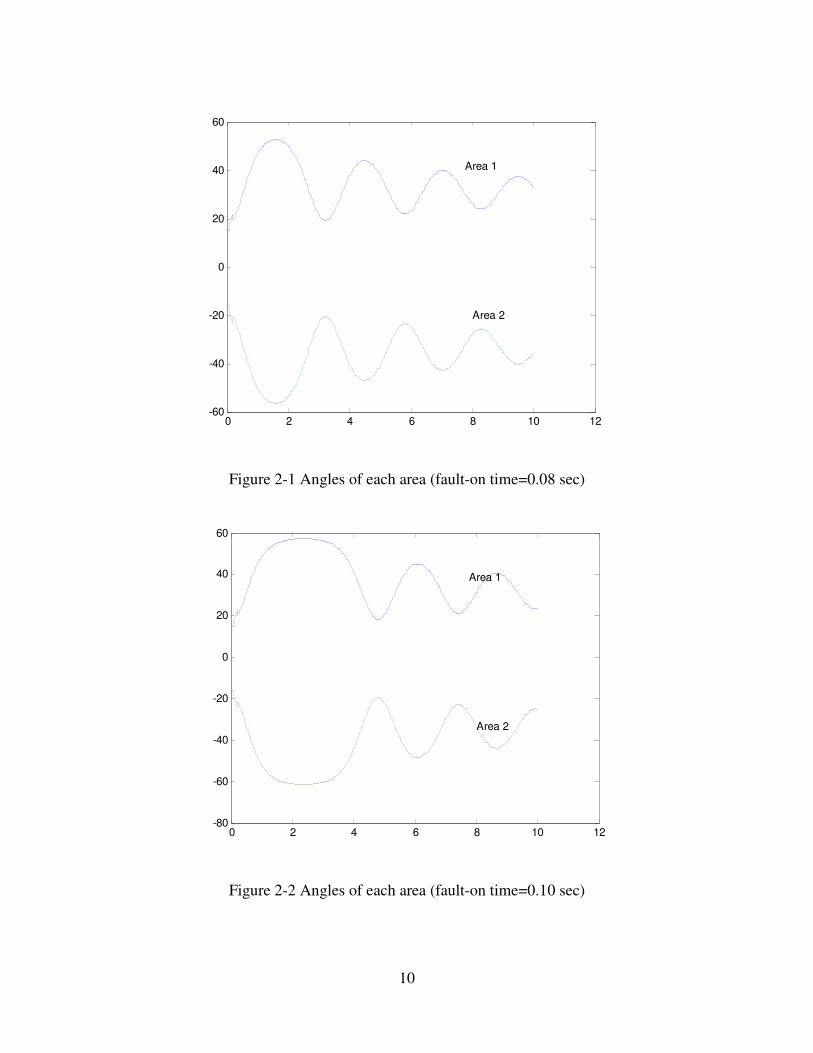
Figure 2-1 Angles of each area (fault-on time=0.08 sec) ......................................... 10
Figure 2-2 Angles of each area (fault-on time=0.10 sec) ......................................... 10
Figure 2-3 Angles of each area (fault-on time=0.11 sec) ......................................... 11
Figure 2-4 Angles of area 1 (fault-on time=0.11 sec)............................................... 11
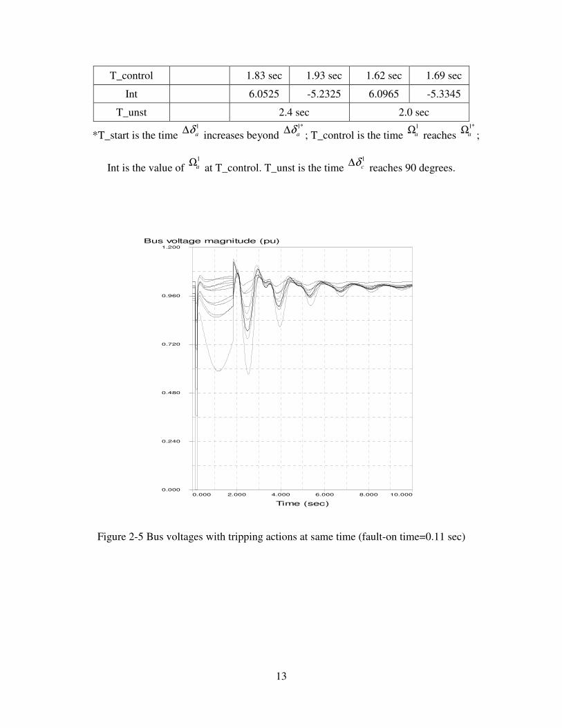
Figure 2-5 Bus voltages with tripping actions at same time (fault-on time=0.11 sec)
........................................................................................................................... 13
Figure 2-6 Bus voltages with tripping actions in turn (fault-on time=0.11 sec)....... 14
Figure 2-7 comparison of two ways to compute cδ (fault-on time=0.11 sec) ......... 15
Figure 2-8 Angles of generators (fault-on time=12 cycles)...................................... 17
Figure 2-9 Angles of generators (fault-on time=13 cycles)...................................... 17
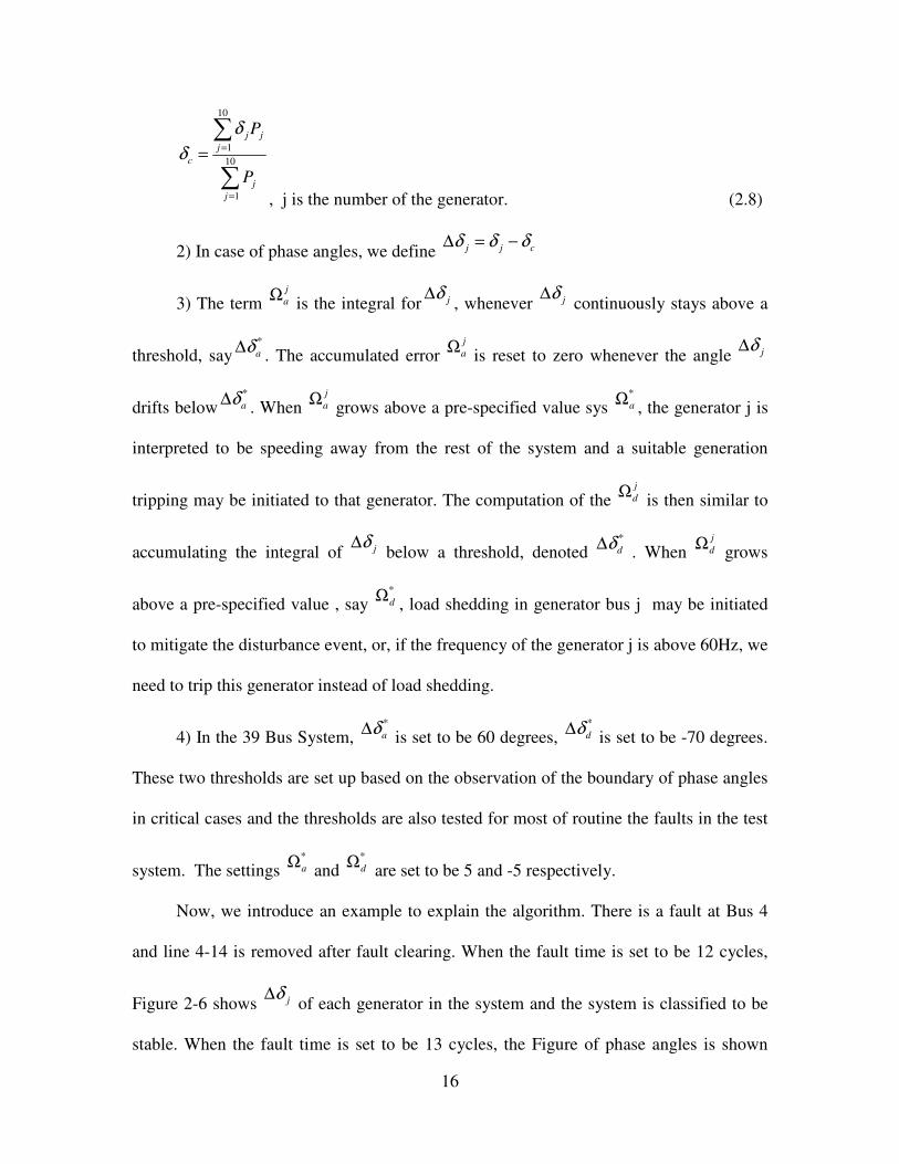
Figure 2-10 Generator speeds (fault-on time=13 cycles) ......................................... 18
Figure 2-11 Bus voltages after tripping Generator 10 (fault-on time=13 cycles)..... 18
Figure 3-1 Angle stability illustration [20] ............................................................... 23
Figure 3-2 Kinetic energy of each generator (fault-on time=10 cycles)................... 26
Figure 3-3 Potential energy of each generator (fault-on time=10 cycles) ................ 26
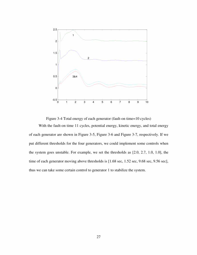
Figure 3-4 Total energy of each generator (fault-on time=10 cycles) ...................... 27
Figure 3-5 Kinetic energy of each generator (fault-on time=11 cycles)................... 28
Figure 3-6 Potential energy of each generator (fault-on time=11 cycles) ................ 28
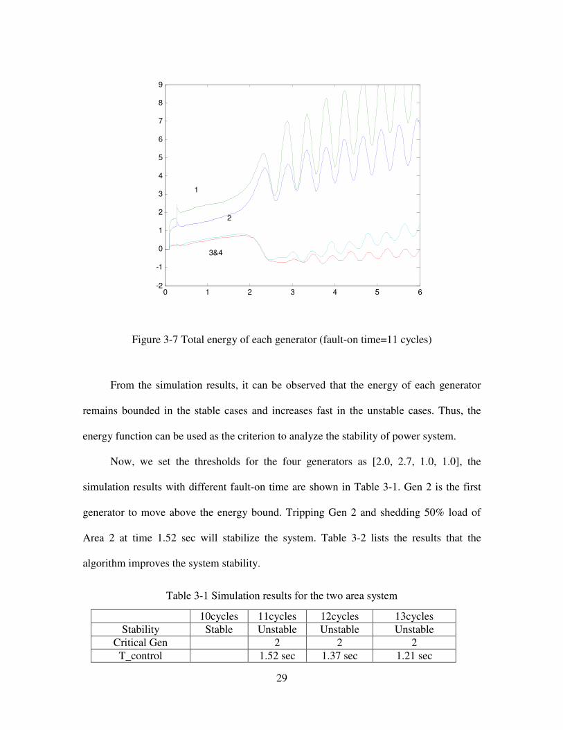
Figure 3-7 Total energy of each generator (fault-on time=11 cycles) ...................... 29
Figure 3-8 Potential energy of each generator (fault-on time=12 cycles) ................ 31
Figure 3-9 Kinetic energy of each generator (fault-on time=12 cycles)................... 31
Figure 3-10 Total energy of each generator (fault-on time=12 cycles) .................... 32
Page 10
x
Figure 3-11 Potential energy of each generator (fault-on time=13 cycles) .............. 32
Figure 3-12 Kinetic energy of each generator (fault-on time=13 cycles)................. 33
Figure 3-13 Total energy of each generator (fault-on time=13 cycles) .................... 33
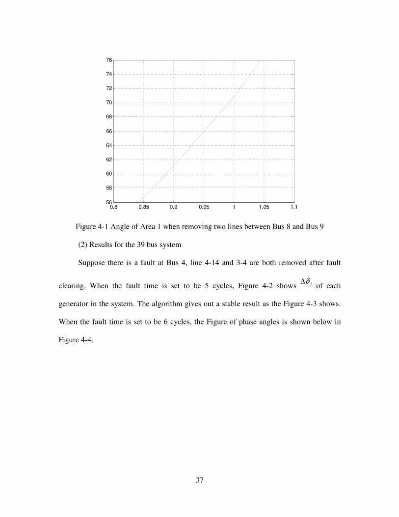
Figure 4-1 Angle of Area 1 when removing two lines between Bus 8 and Bus 9.... 37
Figure 4-2 Angles of generators (fault-on time=5 cycles)........................................ 38
Figure 4-3 Angles of generators (fault-on time=6 cycles)....................................... 38
Figure 4-4 Bus voltages after tripping generator (fault-on time=6 cycles) .............. 39
Figure 4-5 Bus voltages after tripping generator (communication time considered) 43
Figure 4-6 Total energy of each generator removing two lines between Bus 8 and
Bus 9 ................................................................................................................. 45
Figure 4-7 Angles of generators without governors ................................................. 49
Figure 4-8 Total energy of each generator without governors ................................. 50
Figure 4-9 Generator speeds without governors ....................................................... 51
Figure 4-10 Frequency of generators when tripping Gen 2 and Gen 4 .................... 51
Figure 4-11 Angles of generators when tripping Gen 2 and Gen 4 .......................... 52
Figure 4-12 Total energy of each generator when tripping Gen 2 and Gen 4 .......... 52
Figure 4-13 Frequency of generators after load shedding ........................................ 53
Page 11
1
CHAPTER 1 INTRODUCTION
The dynamic responses of power systems can vary over vastly different timescales,
ranging from milliseconds to minutes and even hours. For each type of these dynamic
phenomena, separate controllers have been designed to ensure uninterrupted reliable
operation of the electric power grid that consists of transmission lines, synchronous
machines and consumer loads. The basic control actions, such as the ultra fast power
system protection as well as the slower excitation and governor controls, have been well
developed over the previous decades [5][6]. In the past, the power systems were designed
so that most of the controls were based on local measurements. But on the other hand,
during severely stressed cases, the local control schemes can potentially work against
each other, gradually pushing the system towards cascading outages. Under such severe
and unusual opening conditions, local controls alone can not solve the system security
problems. There have been many recent instances of large-scale blackouts all over the
world [1-4]. These blackouts point to the need for wide-area controls since the blackouts
have highlighted the limitations of the local-based actions.
Power systems are large interconnected nonlinear systems where system wide
instabilities or collapses do occur over time. Accordingly, operator actions together with
automatic control actions are designed to prevent or minimize the damage caused by such
outages. The power-flows across distant parts of the system have been growing steadily
to meet the ever increasing consumer demands. But, the investment into new
transmission lines has been limited due to economic as well as environmental concerns.
Therefore, the steady growth of consumer demands is gradually stressing the electric
Page 12
2
power system more and more. As a result, the system operation can find itself close to or
outside the secure operating limits under severe contingencies.
From the technology perspective, there has been spectacular growth in the past
twenty years from advances in computer and communication sciences. These advances
provide the opportunity for feasible and economical implementation of wide-area
controls in the electric power system.
Wide-area measurement and control systems present a new solution which can be
integrated easily and cost effectively into the power grid. A wide-area control system can
provide the ability to increase the power transmission capability and also improve the
system reliability. Many recent publications have analyzed the requirements and designs
of wide-area controls. The setup and applications of comprehensive wide-area systems
are introduced in [7-9]. The whole new control system can identify critical situations and
determine appropriate remedial actions. The identification together with the actions can
be notified to the operator, and closed loop fast control actions can also be taken
automatically depending on the time frame of the event.
One of the earliest applications of wide-area feedback control in the power system
is the load frequency control [10-12] that was developed in the 1970’s. Any imbalance
between generation and load will cause the deviation of the system frequency away from
the nominal 60 Hz. A secondary control loop, called the Automatic Generation Control,
(AGC), coordinates the individual governor responses of the generators to regulate the
system frequency and also maintain the power exchanges between several control areas.
The control center gathers the relevant frequency and power-flow information from
across the control area and sends the appropriate set point adjustments for each of the
Page 13
3
governor units in the AGC control loop. This AGC control is a slow control system
where the wide-area control adjustments are changed every 15 to 30 seconds or so.
The wide-area controls for the voltage control called Secondary Voltage Control
schemes are proposed in [13-17]. These papers present control schemes designed to
manage voltage and reactive power on a wide network area. The main objective of the
secondary voltage control is to adjust and to maintain the voltage profile inside a network
area. Another objective is the control of reactive generation and flows. This type of
control includes the modification of the set-point values of Automatic Voltage Regulation
(AVR), the switching of compensation devices, and the change of tap position on
transformers. The voltages of key buses are monitored and the control voltage set-points
are sent to the local voltage controllers. New approaches for automatic voltage control
was proposed in [18] that was motivated toward implementation in the transmission
network operated by the Bonneville Power Administration (BPA) in the Pacific
Northwest. Again, the secondary voltage control is also a slow control system with time
constants ranging from 30 seconds to several minutes.
Advanced protection schemes called Special Protection Schemes (SPS’s) or
Remedial Action Schemes (RAS’s) have also been developed in recent years. These
schemes are designed to detect abnormal system conditions such as simultaneous loss of
multiple transmission lines and to take predetermined corrective action to prevent the
system wide instability. RAS schemes involve actions such as generation tripping, load
shedding, capacitor insertion or transformer tap blocking, which are enforced at remote
substations away from the fault location or other events. The use of SPS/RAS can
increase the stability of power systems, especially for specific multiple line openings and
Page 14
4
severe situations if they are designed properly. But these schemes are not flexible, since
they require dedicated communication links and extensive offline calculations. In [19], a
method for an adaptive RAS was proposed. The method calculates the difference of
potential energy to determine each RAS action to increase the stability of the system,
based on the transient energy analysis.
Most of current algorithms used in wide-area control are based on measurements
of bus voltages and generator reactive power. Actually, it will be more effective to use
the phase angle measurements to detect the angle instability, especially, the first swing
instability in power systems [20]. Fast exchange of Phasor Measurements Units (PMU)
among West Electricity Coordination Control (WECC) utilities is being pursued, and it is
reasonable to assume the availability of system wide phase angle information (from
specific PMU locations) in the near future [21]. This thesis proposes new algorithms that
detect and mitigate transient instability by utilizing the phase angle measurements and
frequency measurements of critical generator bus high side voltages from across the
entire power system.
The main contributions of this thesis are listed as follows:
(1) A new algorithm based on the concept of the wide-area control using the phase
angle measurements is proposed and the algorithm is tested in small standard test power
systems. General conclusions drawn from the test systems will be helpful to study the
larger power system.
(2) Extending the first algorithm, the idea of using approximate energy functions to
detect the system instability in a real-time environment is carried out. The second
algorithm is also tested in the two area system and the 39 bus test system.
Page 15
5
All the simulations mentioned in this thesis are done using the Transient Security
Assessment Tool (TSAT). TSAT is a software tool jointly developed by Powertech Labs
Inc. and Nanjing Automation Institute.
The thesis is organized as follows. The algorithm using the system wide phase
angles is described in Chapter 2, and the simulation results are also illustrated in this
chapter. In Chapter 3, the second algorithm using the concept of real-time energy
function is introduced together with the simulation results. The two algorithms are
compared and analyzed in Chapter 4. In the last chapter, conclusions of this thesis are
drawn and some future work is suggested.
Page 16
6
CHAPTER 2 ALGORITHM USING THE PHASE ANGLE
2.1 INTRODUCTION
A first version of the phase angle based algorithm was postulated in Appendix 3 of
the recent paper [21]. This chapter will discusses the new algorithm in more detail along
with illustrative examples on standard IEEE test systems. These algorithms thus extend
the framework of Wide-Area Control Systems (WACS) controller previously developed
at Bonneville Power Administration and Washington State University by including phase
angles into the algorithm computations.
2.2 ALGORITHM
The proposed algorithm extends the concept of the voltage-based algorithm Vmag
from [21] into consideration of the phase angle measurements. At present, the algorithm
analyzes the phase angles in two stages: 1) the angle stability within each control area,
and 2) the angle stability of the entire large system. The principle in each step is similar.
First, let us recall the definition of the Center of Angles (COA) [5],
∑
∑
=
=
−
=N
i
i
i
N
i
i
COA
H
H
1
1
δ
δ (2.1)
where −
iδ is the internal machine rotor angle and iH is the respective generator
inertia time constant. Since the internal machine rotor angle can not be directly measured,
we approximate the internal angle with the phase angle of the high side bus voltage which
is normally monitored by synchrophasors. Similarly, the inertia time constant iH in (2.1)
is difficult to access in real-time. Therefore, we substitute the weights defined by the
Page 17
7
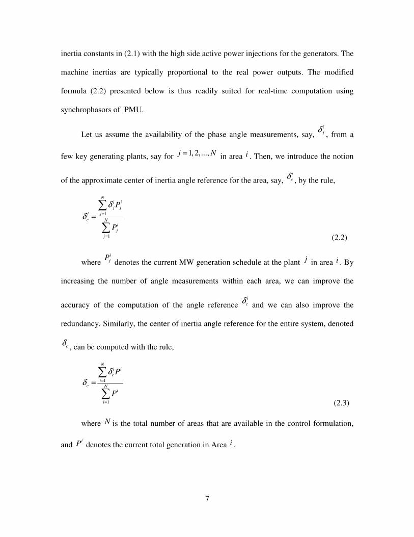
inertia constants in (2.1) with the high side active power injections for the generators. The
machine inertias are typically proportional to the real power outputs. The modified
formula (2.2) presented below is thus readily suited for real-time computation using
synchrophasors of PMU.
Let us assume the availability of the phase angle measurements, say, i
jδ, from a
few key generating plants, say for 1, 2,...,j N= in area i . Then, we introduce the notion
of the approximate center of inertia angle reference for the area, say, i
cδ
, by the rule,
1
1
Ni i
j j
ji
c Ni
j
j
P
P
δ
δ=
=
=
∑
∑ (2.2)
where i
jP denotes the current MW generation schedule at the plant j in area i . By
increasing the number of angle measurements within each area, we can improve the
accuracy of the computation of the angle reference i
cδ
and we can also improve the
redundancy. Similarly, the center of inertia angle reference for the entire system, denoted
cδ
, can be computed with the rule,
1
1
Ni i
c
ic N
i
i
P
P
δ
δ =
=
=
∑
∑ (2.3)
where N is the total number of areas that are available in the control formulation,
and iP denotes the current total generation in Area i .
Page 18
8
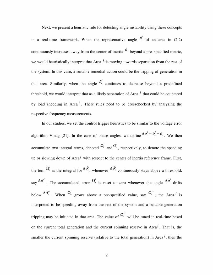
Next, we present a heuristic rule for detecting angle instability using these concepts
in a real-time framework. When the representative angle i
cδ
of an area in (2.2)
continuously increases away from the center of inertia cδ
beyond a pre–specified metric,
we would heuristically interpret that Area i is moving towards separation from the rest of
the system. In this case, a suitable remedial action could be the tripping of generation in
that area. Similarly, when the angle i
cδ
continues to decrease beyond a predefined
threshold, we would interpret that as a likely separation of Area i that could be countered
by load shedding in Area i . There rules need to be crosschecked by analyzing the
respective frequency measurements.
In our studies, we set the control trigger heuristics to be similar to the voltage error
algorithm Vmag [21]. In the case of phase angles, we definei i
c c cδ δ δ∆ = −
. We then
accumulate two integral terms, denoted i
aΩ
andi
dΩ
, respectively, to denote the speeding
up or slowing down of Area i with respect to the center of inertia reference frame. First,
the termi
aΩ
is the integral fori
cδ∆
, whenever i
cδ∆
continuously stays above a threshold,
say*i
cδ∆
. The accumulated error i
aΩ
is reset to zero whenever the angle i
cδ∆
drifts
below*i
aδ∆
. When i
aΩ
grows above a pre-specified value, say *i
aΩ
, the Area i is
interpreted to be speeding away from the rest of the system and a suitable generation
tripping may be initiated in that area. The value of *i
aΩ
will be tuned in real-time based
on the current total generation and the current spinning reserve in Area i . That is, the
smaller the current spinning reserve (relative to the total generation) in Area i , then the
Page 19
9
lower the threshold value for *i
aΩ
. The computation of the i
dΩ
is then similar to
accumulating the integral of i
cδ∆
below a threshold, denoted *i
dδ∆
. When i
dΩ
grows
above a pre-specified value, say *i
dΩ
, load shedding in Area i may be initiated to mitigate
the disturbance event.
2.3 ILLUSTRATION OF THE ALGORITHM USING THE TWO AREA SYSTEM
We implement the above algorithm in the two area system (the diagram of the two
area system is shown in Appendix A). The system is simply divided into two areas with
Gen 1 and Gen 2 in Area 1, Gen 3 and Gen 4 in Area 2, respectively. We define
1 21 1 1 1 2
1 2
G Gc
G G
P P
P P
δ δδ
+=
+ (2.4)
43
4
4
23
31
22
GG
GG
cPP
PP
+
+=
δδδ (2.5)
Where1
1δ,
2
1δ,
3
2δ,
4
2δ are the phase angles of the bus voltage of the four
generators, respectively. Also, we define
4321
4
4
23
3
22
2
11
1
1
GGGG
GGGG
cPPPP
PPPP
+++
+++=
δδδδδ (2.6)
1 1
c c cδ δ δ∆ = −
,2 2
c c cδ δ δ∆ = −
(2.7)
When we apply a three phase fault at BUS 8 and after some certain time we clear
the fault and remove three of the four lines between BUS 7 and BUS 8 at time 0.1 sec, the
details of the simulation results are shown below. When the fault-on time is set to be 0.08
sec, 0.10 sec, and 0.11 sec, the curves of 1
cδ∆
and 2
cδ∆
are shown in Figure 2-1, Figure
2-2 and Figure 2-3, respectively. Figure 2-4 shows the curve of 1
cδ∆
near 60 degrees.
Page 20
10
0 2 4 6 8 10 12-60
-40
-20
0
20
40
60
Area 1
Area 2
Figure 2-1 Angles of each area (fault-on time=0.08 sec)
0 2 4 6 8 10 12-80
-60
-40
-20
0
20
40
60
Area 1
Area 2
Figure 2-2 Angles of each area (fault-on time=0.10 sec)
Page 21
11
0 1 2 3 4 5 6-2500
-2000
-1500
-1000
-500
0
500
1000
1500
2000
2500
Area 1
Area 2
Figure 2-3 Angles of each area (fault-on time=0.11 sec)
1.5 1.55 1.6 1.65 1.7 1.75 1.8 1.85 1.9 1.95 256
57
58
59
60
61
62
63
64
65
66
Figure 2-4 Angles of area 1 (fault-on time=0.11 sec)
Page 22
12
From the cases above, we could say that 0.10 sec is the critical fault time for this
three phase fault on Bus8. Looking into Figure 2-2, we could find that the maximum
value of 1
cδ∆
is 57.3 degrees and the minimum value of 2
cδ∆
is -61.5 degrees. Therefore,
we set *
aδ∆ =60 degrees, *
dδ∆ =-65 degrees, *
aΩ =5 and *
dΩ =-5. Simulation results with
different fault-on time are shown in Table 2-1. From the results, we could say Area 1 is
moving away from the system earlier than Area 2. When we try to trip some generation
of Area 1, we find that the generation tripping action by itself is not enough to stabilize
the system. Thus, we add some load shedding action in Area 2. We trip Gen 1 and 50%
of the load at Bus 9 at time 1.83 sec for the second case in Table 2-1. The system can be
stable as shown in Figure 2-5. Also, if we trip Gen 1 at time 1.83 sec and 50% load at Bus
9 at time 1.93 sec, the system can be stabilized as shown in Figure 2-6. As a result, the
new algorithm works for this example in the two area system. Table 2-2 summarizes the
benefits provided by the algorithm in improving the transient stability. Taking the first
case as example, the critical clearing time without the proposed control is 0.10 seconds
(the first entry in Table 2-1). The system becomes transient stable for the clearing time of
0.11 seconds as well as 0.12 seconds. With the automatic generation tripping control as
proposed, the critical clearing time improves to 0.14 seconds. Compared to the 0.10
seconds for the original system with no control, the automatic controller as proposed
provides an improved critical clearing time by a margin of 0.04 seconds (2.4 cycles).
Table 2-1 Simulation results for the two area system
Fault Time 0.10 sec 0.11 sec 0.12 sec
Stability Stable Unstable Unstable
Area Area1 Area2 Area1 Area2
T_start 1.73 sec 1.89 sec 1.52 sec 1.61sec
Page 23
13
T_control 1.83 sec 1.93 sec 1.62 sec 1.69 sec
Int 6.0525 -5.2325 6.0965 -5.3345
T_unst 2.4 sec 2.0 sec
*T_start is the time 1
aδ∆
increases beyond 1*
aδ∆
; T_control is the time 1
aΩ
reaches 1*
aΩ
;
Int is the value of 1
aΩ
at T_control. T_unst is the time 1
cδ∆
reaches 90 degrees.
Bus voltage magnitude (pu)
Time (sec)
0.000 2.000 4.000 6.000 8.000 10.000
0.000
0.240
0.480
0.720
0.960
1.200
Figure 2-5 Bus voltages with tripping actions at same time (fault-on time=0.11 sec)
Page 24
14
Bus voltage magnitude (pu)
Time (sec)
0.000 2.000 4.000 6.000 8.00010.000
0.400
0.560
0.720
0.880
1.040
1.200
Figure 2-6 Bus voltages with tripping actions in turn (fault-on time=0.11 sec)
Table 2-2 Improvement on the system stability
Fault Bus Line
Removed
Fault Time
(cycle)
improvement
8 7-8 2.4
7 7-8 1.8
Tests in two area system lead to some discussions of the new algorithm.
(1) If we use inertia constants to compute cδ as formula (2.1) shows, with the 0.11
sec-fault time, Figure 2-7 shows the comparison of the two methods. It shows that the
substitution with power output to compute cδ is reasonable.
Page 25
15
1.5 1.55 1.6 1.65 1.7 1.75 1.8 1.85 1.9 1.95 256
57
58
59
60
61
62
63
64
65
66
use "P"
use "H"
Figure 2-7 comparison of two ways to compute cδ (fault-on time=0.11 sec)
(2) The thresholds are set up based on the critical cases and they need to be tuned
in order to make the algorithm work reasonably for diverse conditions.
(3) Control actions such as the generation tripping in the accelerating area or load
shedding in the decelerating area are the normal methods in system protection. But, the
tripping or shedding amounts still need to be determined from further studies in future
research works.
2.4 IMPLEMENTATION OF THE ALGORITHM IN THE 39 BUS SYSTEM
We also implement the algorithm in the 39 Bus System (the diagram of the 39 bus
system is shown in Appendix B). In this system, we treat each generator bus is a
individual control bus, thus, the algorithm is re-written as following:
1) The COA of the system is defined as,
Page 26
16
∑
∑
=
==
10
1
10
1
j
j
j
jj
c
P
Pδ
δ
, j is the number of the generator. (2.8)
2) In case of phase angles, we define cjj δδδ −=∆
3) The term j
aΩ is the integral for jδ∆
, whenever jδ∆ continuously stays above a
threshold, say*
aδ∆. The accumulated error
j
aΩ is reset to zero whenever the angle jδ∆
drifts below*
aδ∆. When
j
aΩ grows above a pre-specified value sys
*
aΩ, the generator j is
interpreted to be speeding away from the rest of the system and a suitable generation
tripping may be initiated to that generator. The computation of the j
dΩ is then similar to
accumulating the integral of jδ∆ below a threshold, denoted
*
dδ∆ . When
j
dΩ grows
above a pre-specified value , say *
dΩ, load shedding in generator bus j may be initiated
to mitigate the disturbance event, or, if the frequency of the generator j is above 60Hz, we
need to trip this generator instead of load shedding.
4) In the 39 Bus System, *
aδ∆ is set to be 60 degrees,
*
dδ∆ is set to be -70 degrees.
These two thresholds are set up based on the observation of the boundary of phase angles
in critical cases and the thresholds are also tested for most of routine the faults in the test
system. The settings *
aΩ and
*
dΩ are set to be 5 and -5 respectively.
Now, we introduce an example to explain the algorithm. There is a fault at Bus 4
and line 4-14 is removed after fault clearing. When the fault time is set to be 12 cycles,
Figure 2-6 shows jδ∆ of each generator in the system and the system is classified to be
stable. When the fault time is set to be 13 cycles, the Figure of phase angles is shown
Page 27
17
below (Figure 2-7).
Figure 2-8 Angles of generators (fault-on time=12 cycles)
Figure 2-9 Angles of generators (fault-on time=13 cycles)
Page 28
18
From the algorithm, generator 10 is the first to move away from the COA, the
control time is 0.76 sec. So we trip Gen 10 to stabilize the system as the frequency of Gen
10 is above 60 Hz (Figure 2-7). The figure of the system bus voltages is shown below
(Figure 2-8).
Generator speed (Hz)
Time (sec)
0.000 0.383 0.767 1.150 1.534 1.91759.900
61.140
62.380
63.620
64.860
66.100
Figure 2-10 Generator speeds (fault-on time=13 cycles)
Figure 2-11 Bus voltages after tripping
Generator 10 (fault-on time=13 cycles)
The following table (table 2-3) summarizes the simulation results for various single
line outages. The fault time of each fault is the critical time when the system becomes
unstable. The Gen tripped and tripping time is the generator needed to be tripped and the
Bus voltage magnitude (pu)
Time (sec)
0.000 2.000 4.000 6.000 8.000 10.0000.000
0.240
0.480
0.720
0.960
1.200
Page 29
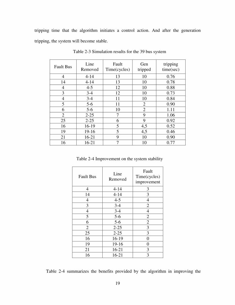
19
tripping time that the algorithm initiates a control action. And after the generation
tripping, the system will become stable.
Table 2-3 Simulation results for the 39 bus system
Fault Bus Line
Removed
Fault
Time(cycles)
Gen
tripped
tripping
time(sec)
4 4-14 13 10 0.76
14 4-14 13 10 0.78
4 4-5 12 10 0.88
3 3-4 12 10 0.73
4 3-4 11 10 0.84
5 5-6 11 2 0.90
6 5-6 10 2 1.11
2 2-25 7 9 1.06
25 2-25 6 9 0.92
16 16-19 5 4,5 0.52
19 19-16 5 4,5 0.46
21 16-21 9 10 0.90
16 16-21 7 10 0.77
Table 2-4 Improvement on the system stability
Fault Bus Line
Removed
Fault
Time(cycles)
improvement
4 4-14 3
14 4-14 3
4 4-5 4
3 3-4 2
4 3-4 4
5 5-6 2
6 5-6 2
2 2-25 3
25 2-25 3
16 16-19 0
19 19-16 0
21 16-21 3
16 16-21 3
Table 2-4 summarizes the benefits provided by the algorithm in improving the
Page 30
20
transient stability. For instance, let us consider the first contingency in Table 2-4, the
three phase fault on Bus 4 and the loss of line 4-14. The critical clearing time without the
proposed control is 12 cycles. For the 13 cycles-clearing time case, the phase angle based
algorithm identifies Gen 10 as the critical generator and a trip signal is issued by the
control to Gen 10 at 0.76 seconds (first entry of Table 2-3). Assuming that the generator
is tripped by the proposed controller, the system becomes transient stable for the clearing
time of 13 cycles as well as 14 cycles. With the automatic generation tripping control as
proposed, the critical clearing time improves to 15 cycles. Compared to the 12 cycles for
the original system with no control, the automatic controller as propose provides an
improved critical clearing time by a margin of 3 cycles. Table 2-4 thus illustrates the
effectiveness of the algorithm in detecting and mitigating transient stability contingencies
in various parts of the system.
It is important to point out that the control decision is entirely based on the
measured phase angles and the controller does not know what outage resulted in the
observed phase angle responses. This is a purely response based algorithm in the spirit of
the previous algorithms in [21].
From Table 2-4, the controller based only on phase angle improves the system
security for all excepting two outages. For the two exceptions, the controller does not
cause negative margins or effects. Thus, the controller does appear to be effective for the
39 bus system.
Page 31
21
2.5 CONCLUSION
This chapter presents the algorithm for processing of phase angle measurements
from across the system to decide whether any part or control area within the system is
speeding away from the rest. When the angle separations go above preset thresholds,
remedial actions such as generation and load tripping are ordered by the stability
controller to keep the areas in synchronism. This new algorithm can detect and mitigate
transient instability by utilizing the phase angle measurements of critical generator bus
voltages. The algorithm can be realized in the simulation of the two area system and the
39 bus System. The thresholds are set up based on the critical cases and tuned in order to
make the algorithm work for the whole system. Control actions such as Tripping
generation in accelerating area or shedding load in decelerating area are the normal
methods in system protection. But, if the frequencies of the generators in decelerating
area are above 60Hz, we need to trip generation in this area instead of load shedding. The
tripping or shedding amounts still need further studies in future research work.
Page 32
22
CHAPTER 3 ALGORITHM USING THE ENERGY FUNCTION
3.1 BACKGROUND
Transient energy methods are mathematical techniques for analyzing the power
system dynamics due to excursions in voltage phase angles and their magnitudes. The
energy associated with the deviation from system equilibrium point is quantified as a
kinetic energy function (KE) that is related to changes in rotor speeds and a potential
energy function (PE) that is connected with changes in relative rotor phase angles. In our
research, we are trying to establish the relation between the system transient behavior and
the measurements from PMU. The transient energy method is used to analyze the system
stability so that PMU based measurements can be used for detecting the system instability
in real-time, and for activating suitable control actions.
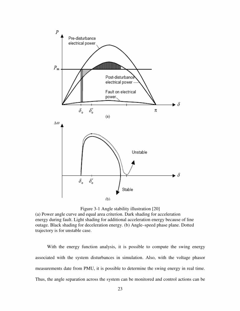
Figure 3-1 illustrates the equal area stability criterion for “first swing” stability [20].
If the decelerating area (energy) above the mechanical power load line is greater than the
accelerating area below the load line, stability can be maintained.
Transient energy analysis has been developed with substantial advances in recent
years. The method to evaluate the transient response of a power system following a large
disturbance was proposed in [24]. [25], [26]. [27] used energy functions to quantify the
energy of a system disturbance. In 1982, Vitta1 [28] introduced the idea of an individual
machine’s energy function, and in 1988 Stanton used transient energy functions of an
individual generator, to assess instability of individual sites [29-31]. The Energy
Functions are fully described in references [26],[28],[30] and [31]. The algorithm using
energy function to detect system instability based on PMU can be found in [32], where
the definition of critical energy was carried out as criterion of system stability.
Page 33
23
Figure 3-1 Angle stability illustration [20]
(a) Power angle curve and equal area criterion. Dark shading for acceleration
energy during fault. Light shading for additional acceleration energy because of line
outage. Black shading for deceleration energy. (b) Angle–speed phase plane. Dotted
trajectory is for unstable case.
With the energy function analysis, it is possible to compute the swing energy
associated with the system disturbances in simulation. Also, with the voltage phasor
measurements date from PMU, it is possible to determine the swing energy in real time.
Thus, the angle separation across the system can be monitored and control actions can be
Page 34
24
taken to stabilize the system. In [32], the critical energy of each generator in the system is
predetermined by the off-line computations. In real-time simulation, the computation of
the kinetic energy function of each generator is used to detect whether the generators are
remain in boundary in order to analyze the system stability. The recent paper [33]
proposed a synchronous phasor data based energy function analysis in typical power
transfer path with two generators. In our research, we carry out the potential energy
function together with the kinetic energy function to define the total energy of each
generator in the system. Computation of both energy functions in real-time is used to
detect the system instability for the large power system with no restrictions on the size of
the system or on the number of generators.
3.2 ALGORITHM
A Partial Energy Function is one that computes the transient energy of a single
generator (or subsystem) in a multimachine system. In Partial Energy Function analysis,
the transient energy for generator i , is defined as the integral of the power accelerating
the generator’s rotor,
∫ −=
i
iii PGPTPEθ
)(
(3.1)
Transient energy can be resolved into Kinetic Energy, by
2)1( −= iii HKE ω (3.2)
where ,
iω = rotor speed of generator
iH = Inertia constant of generator
Page 35
25
iPT = torque
iPG = MW generation of generator
iθ=rotor angle
In our approach, we propose the real-time synchronous total energy of each
generator in the system as the criterion to analyze the stability of the system. We define
the total energy of each generator as iTE,
where, iii PEKETE +=. (3.3)
Now, we simply use iTE to analyze the stability of the system by observing
whether iTE are remaining bounded. In practice, it is not convenient to get
measurements of the rotor speed or angle. iω~
and iθ~
, representing the generator high side
bus frequency and voltage angle, respectively, are introduced into the simulation.
3.3 ILLUSTRATION OF THE ALGORITHM IN THE TWO AREA SYSTEM
In the two area system, when we apply a three phase fault at BUS 8 and after some
certain time we clear the fault and remove three of the four lines between BUS 7 and
BUS 8 at time 0.1 sec, the details of the simulation results are shown below.
With the fault-on time 10 cycles, potential energy, kinetic energy, and total energy
of each generator are shown in Figure 3-2, Figure 3-3 and Figure 3-4, respectively.
Page 36
26
0 1 2 3 4 5 6 7 8 9 100
0.1
0.2
0.3
0.4
0.5
0.6
1&2
3&4
Figure 3-2 Kinetic energy of each generator (fault-on time=10 cycles)
0 1 2 3 4 5 6 7 8 9 10-0.5
0
0.5
1
1.5
2
2.5
1
2
3&4
Figure 3-3 Potential energy of each generator (fault-on time=10 cycles)
Page 37
27
0 1 2 3 4 5 6 7 8 9 10-0.5
0
0.5
1
1.5
2
2.5
1
2
3&4
Figure 3-4 Total energy of each generator (fault-on time=10 cycles)
With the fault-on time 11 cycles, potential energy, kinetic energy, and total energy
of each generator are shown in Figure 3-5, Figure 3-6 and Figure 3-7, respectively. If we
put different thresholds for the four generators, we could implement some controls when
the system goes unstable. For example, we set the thresholds as [2.0, 2.7, 1.0, 1.0], the
time of each generator moving above thresholds is [1.68 sec, 1.52 sec, 9.68 sec, 9.56 sec],
thus we can take some certain control to generator 1 to stabilize the system.
Page 38
28
0 1 2 3 4 5 6-1
-0.5
0
0.5
1
1.5
2
2.5
3
3.5
4
1&2
3&4
Figure 3-5 Kinetic energy of each generator (fault-on time=11 cycles)
0 1 2 3 4 5 6-2
-1
0
1
2
3
4
5
6
1
2
3&4
Figure 3-6 Potential energy of each generator (fault-on time=11 cycles)
Page 39
29
0 1 2 3 4 5 6-2
-1
0
1
2
3
4
5
6
7
8
9
1
2
3&4
Figure 3-7 Total energy of each generator (fault-on time=11 cycles)
From the simulation results, it can be observed that the energy of each generator
remains bounded in the stable cases and increases fast in the unstable cases. Thus, the
energy function can be used as the criterion to analyze the stability of power system.
Now, we set the thresholds for the four generators as [2.0, 2.7, 1.0, 1.0], the
simulation results with different fault-on time are shown in Table 3-1. Gen 2 is the first
generator to move above the energy bound. Tripping Gen 2 and shedding 50% load of
Area 2 at time 1.52 sec will stabilize the system. Table 3-2 lists the results that the
algorithm improves the system stability.
Table 3-1 Simulation results for the two area system
10cycles 11cycles 12cycles 13cycles
Stability Stable Unstable Unstable Unstable
Critical Gen 2 2 2
T_control 1.52 sec 1.37 sec 1.21 sec
Page 40
30
Table 3-2 Improvement on the system stability
Fault Bus Line
Removed
Fault
Time(cycles)
improvement
8 7-8 3
7 7-8 2
3.4 IMPLEMENTATION OF THE ALGORITHM IN THE 39 BUS SYSTEM
We also implement the algorithm in the 39 bus System. Now, we introduce an
example to explain the algorithm. There is a fault at Bus 4 and line 4-14 is removed after
fault clearing. With the fault-on time 12 cycles, potential energy, kinetic energy, and total
energy of each generator are shown in Figure 3-8, Figure 3-9 and Figure 3-10,
respectively. With the fault-on time 13 cycles, potential energy, kinetic energy, and total
energy of each generator are shown in Figure 3-11, Figure 3-12 and Figure 3-13,
respectively. Therefore, if we put different thresholds to the generators, we could
implement some controls when the system goes unstable.
Page 41
31
0 1 2 3 4 5 6 7 8 9 10-5
0
5
10
15
20
25
Figure 3-8 Potential energy of each generator (fault-on time=12 cycles)
0 1 2 3 4 5 6 7 8 9 100
5
10
15
20
25
Figure 3-9 Kinetic energy of each generator (fault-on time=12 cycles)
Page 42
32
0 1 2 3 4 5 6 7 8 9 100
5
10
15
20
25
30
35
40
45
50
Figure 3-10 Total energy of each generator (fault-on time=12 cycles)
0 0.5 1 1.5 2 2.5 30
5
10
15
20
25
30
35
40
45
50
Figure 3-11 Potential energy of each generator (fault-on time=13 cycles)
Page 43
33
0 0.5 1 1.5 2 2.5 30
10
20
30
40
50
60
Figure 3-12 Kinetic energy of each generator (fault-on time=13 cycles)
0 0.5 1 1.5 2 2.5 30
20
40
60
80
100
120
Figure 3-13 Total energy of each generator (fault-on time=13 cycles)
Page 44
34
Since Gen 10 is much larger compared to the rest generators in capacities, the
energy bound also needs to be set larger than the rest. For example, we set 50 as the
threshold for Gen 10, 10 for the rest generators. The following table (Table 3-3) shows
the simulation results. The fault time of each fault is the critical time when the system
becomes unstable. The Gen is the critical generator that the algorithm gives out. Table 3-
4 lists the results that the algorithm improves the system stability. Considering the first
contingency in Table 3-4, there is a three phase fault on Bus 4 and line 4-14 is removed
after clearing. The critical clearing time without the proposed control is 12 cycles. For
this case, the energy function based algorithm identifies Gen 10 as the critical generator
and a trip signal is issued by the control to Gen 10 at 1.09 seconds. Assuming that the
generator is tripped by the proposed controller, the system becomes transient stable for
the clearing time of 13 cycles as well as 14 cycles. Compared to the 12 cycles for the
original system with no control, the automatic controller as propose provides an improved
critical clearing time by a margin of 2 cycles. Recalling Table 2-3 and Table 2-4, we
could find the energy function based algorithm consumes more time in identifying system
instability, so that the improvement is not as effective as the angle based algorithm.
Table 3-3 Simulation results for the 39 bus system
Fault Bus Line
Removed
Fault
Time(cycle
s)
Gen tripped tripping
time(sec)
4 4-14 13 10 1.09
14 4-14 13 10 1.13
4 4-5 12 10 1.31
3 3-4 12 10 0.99
4 3-4 11 10 1.03
5 5-6 11 2 1.23
6 5-6 10 2 1.37
2 2-25 7 9 1.41
Page 45
35
25 2-25 6 9 1.32
16 16-19 5 4,5 0.58
19 19-16 5 4,5 0.52
21 16-21 9 10 1.02
16 16-21 7 10 0.92
Table 3-4 Improvement on the system stability
Fault Bus Line
Removed
Fault
Time(cycles)
improvement
4 4-14 2
14 4-14 2
4 4-5 3
3 3-4 1
4 3-4 1
5 5-6 1
6 5-6 1
2 2-25 0
25 2-25 0
16 16-19 0
19 19-16 0
21 16-21 1
16 16-21 1
3.5 CONCLUSION
The work reported in this chapter investigated the ability of energy function based
on synchronized phase angle measurements to identify impending instabilities. The
definition of the potential energy and the kinetic energy carry out new concepts of energy
analysis in real-time large power system control. The new algorithm is tested on both the
two area system and the 39 bus system.
Page 46
36
CHAPTER 4 TESTS USING VARIOUS SIMULATION CONDITIONS
In Chapter 2 and Chapter 3, the two algorithms were proposed and tested in both
the two area system and the 39 bus system. In this Chapter, we discuss variations of the
simulation conditions, load model and the comparison of the two algorithms are carried
out and lead to some conclusions.
4.1 ALGORITHM USING THE PHASE ANGLES
4.1.1 Multiple contingencies
In Chapter 2, the simulation results are based on single three phase fault on buses.
More simulations are listed below with different fault type and conditions.
(1) Results of the two area system
(a) When we apply a three phase fault at BUS 9 and after some certain time we
clear the fault and remove one of the three lines between BUS 8 and BUS 9 at time 0.1
sec, the system will maintain stable even the fault-on time increases to 0.25 sec.
(b) When we remove two of the three lines between BUS 8 and BUS 9 at time 0.1
sec, the system will collapse as the simulation shows. The angle of Area 1 will reach the
threshold at 0.92 sec, and the controller will identify the instability and send out a
tripping signal at 1.00 sec. But since the fault is too severe, the control actions including
generation tripping in Area1 and load shedding in Area 2 will not stabilize the system.
Page 47
37
0.8 0.85 0.9 0.95 1 1.05 1.156
58
60
62
64
66
68
70
72
74
76
Figure 4-1 Angle of Area 1 when removing two lines between Bus 8 and Bus 9
(2) Results for the 39 bus system
Suppose there is a fault at Bus 4, line 4-14 and 3-4 are both removed after fault
clearing. When the fault time is set to be 5 cycles, Figure 4-2 shows jδ∆ of each
generator in the system. The algorithm gives out a stable result as the Figure 4-3 shows.
When the fault time is set to be 6 cycles, the Figure of phase angles is shown below in
Figure 4-4.
Page 48
38
Figure 4-2 Angles of generators (fault-on time=5 cycles)
0 0.2 0.4 0.6 0.8 1 1.2 1.4 1.6 1.8 2-200
0
200
400
600
800
1000
Figure 4-3 Angles of generators (fault-on time=6 cycles)
Page 49
39
Bus voltage magnitude (pu)
Time (sec)
0.000 2.000 4.000 6.000 8.000 10.0000.000
0.240
0.480
0.720
0.960
1.200
Figure 4-4 Bus voltages after tripping generator (fault-on time=6 cycles)
From the algorithm, generator 10 is the first to move away from the COA, the
control time is 1.06 sec. So we trip Gen 10 to stabilize the system as the frequency of Gen
10 is above 60 Hz. The bus voltage Figure of the system is shown left in Figure 4-3. In
this case, the critical clearing time will be improved by 2 cycles for the double
contingency with the proposed angle based algorithm.
4.1.2 Consideration of the load level and the load model
(1) Results of the two area system
We decrease the load in the previous the two area system and get a new power-
flow solution, then we simulate the same fault tested in Chapter 2, the results are shown
in Table 4-1. In this case, when the clearing time is 0.20 seconds, the controller will
Page 50
40
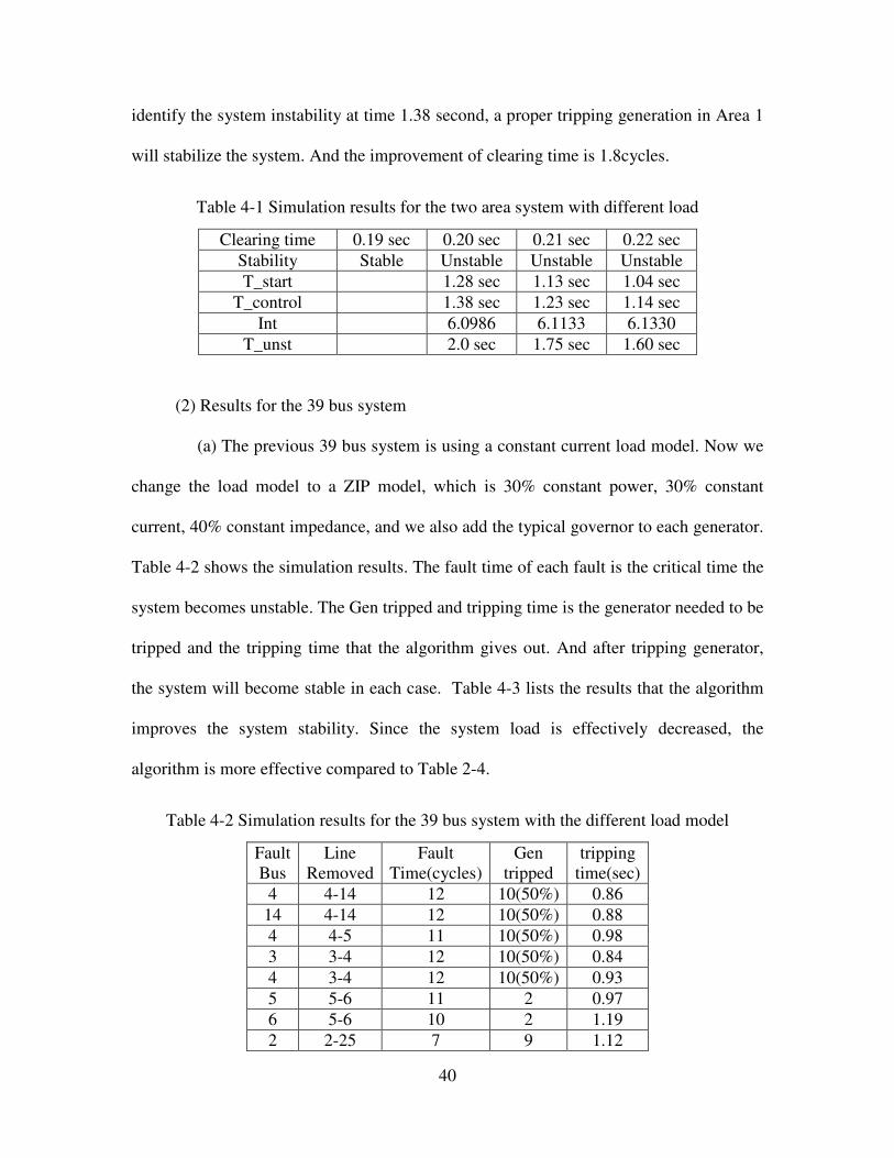
identify the system instability at time 1.38 second, a proper tripping generation in Area 1
will stabilize the system. And the improvement of clearing time is 1.8cycles.
Table 4-1 Simulation results for the two area system with different load
Clearing time 0.19 sec 0.20 sec 0.21 sec 0.22 sec
Stability Stable Unstable Unstable Unstable
T_start 1.28 sec 1.13 sec 1.04 sec
T_control 1.38 sec 1.23 sec 1.14 sec
Int 6.0986 6.1133 6.1330
T_unst 2.0 sec 1.75 sec 1.60 sec
(2) Results for the 39 bus system
(a) The previous 39 bus system is using a constant current load model. Now we
change the load model to a ZIP model, which is 30% constant power, 30% constant
current, 40% constant impedance, and we also add the typical governor to each generator.
Table 4-2 shows the simulation results. The fault time of each fault is the critical time the
system becomes unstable. The Gen tripped and tripping time is the generator needed to be
tripped and the tripping time that the algorithm gives out. And after tripping generator,
the system will become stable in each case. Table 4-3 lists the results that the algorithm
improves the system stability. Since the system load is effectively decreased, the
algorithm is more effective compared to Table 2-4.
Table 4-2 Simulation results for the 39 bus system with the different load model
Fault
Bus
Line
Removed
Fault
Time(cycles)
Gen
tripped
tripping
time(sec)
4 4-14 12 10(50%) 0.86
14 4-14 12 10(50%) 0.88
4 4-5 11 10(50%) 0.98
3 3-4 12 10(50%) 0.84
4 3-4 12 10(50%) 0.93
5 5-6 11 2 0.97
6 5-6 10 2 1.19
2 2-25 7 9 1.12
Page 51
41
25 2-25 6 9 0.98
16 16-19 5 4,5 0.54
19 19-16 5 4,5 0.50
21 16-21 10 10(50%) 0.97
16 16-21 8 10(50%) 0.79
Table 4-3 Improvement on the system stability
Fault
Bus
Line
Removed
Fault
Time(cycles)
improvement
4 4-14 5
14 4-14 5
4 4-5 4
3 3-4 3
4 3-4 4
5 5-6 2
6 5-6 2
2 2-25 4
25 2-25 4
16 16-19 0
19 19-16 0
21 16-21 3
16 16-21 3
(b) Continuing with the previous ZIP (30%, 30%, 40%) load model, we increase the
load level to 120% and distribute the load to each generator of the system. Table 4-4
shows the simulation results. The fault time of each fault is the critical time the system
becomes unstable. Since the system condition is severe, when the first phase angle moves
above the pre-specified threshold, we take a generation tripping in accelerating area; at
the same time, we also add load shedding action in decelerating area. In each unstable
case, Gen 10 is the one which decelerates from COA, so we shed 50% load (600MW) at
the Bus 39 which is the terminal bus of Gen 10 at the time the first angle moves beyond
threshold. Table 4-5 lists the results that the algorithm improves the system stability.
This test shows that the algorithm can still work with a stress system condition.
Page 52
42
Table 4-4 Simulation results for the 39 bus system in a stress condition
Fault
Bus
Line
Removed
Fault
Time(cycles)
Gen
tripped
tripping
time(sec)
4 4-14 7 2,3 0.87
14 4-14 7 2,3 0.86
4 4-5 6 2,3 0.93
3 3-4 7 2,3 0.85
4 3-4 7 2,3 0.95
5 5-6 6 2 0.99
6 5-6 5 2 1.06
2 2-25 6 9 1.05
25 2-25 5 9 0.89
16 16-19 5 4,5 0.53
19 19-16 5 4,5 0.51
21 16-21 7 2,3 0.93
16 16-21 6 2,3 0.81
Table 4-5 Improvement on the system stability
Fault
Bus
Line
Removed
Fault
Time(cycles)
improvement
4 4-14 0
14 4-14 0
4 4-5 1
3 3-4 1
4 3-4 2
5 5-6 1
6 5-6 1
2 2-25 2
25 2-25 2
16 16-19 0
19 19-16 0
21 16-21 1
16 16-21 1
4.1.3 Consideration of the communication time
In real-time control we need to consider the communication time of the control.
Suppose the average communication time from PMU units to control center to be 0.075
sec. Thus, we take this time as 0.15 sec (a round-trip between PMU units and control
Page 53
43
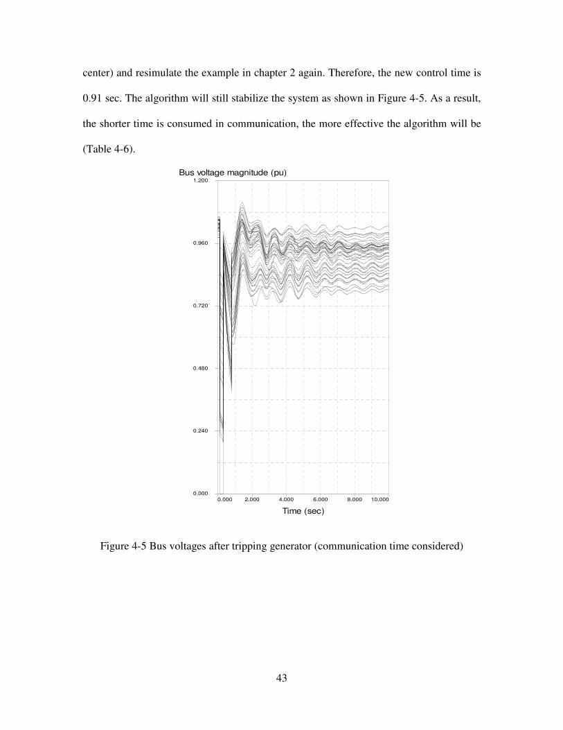
center) and resimulate the example in chapter 2 again. Therefore, the new control time is
0.91 sec. The algorithm will still stabilize the system as shown in Figure 4-5. As a result,
the shorter time is consumed in communication, the more effective the algorithm will be
(Table 4-6).
Bus voltage magnitude (pu)
Time (sec)
0.000 2.000 4.000 6.000 8.000 10.0000.000
0.240
0.480
0.720
0.960
1.200
Figure 4-5 Bus voltages after tripping generator (communication time considered)
Page 54
44
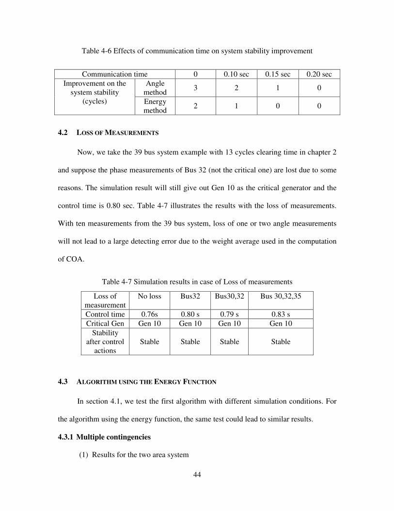
Table 4-6 Effects of communication time on system stability improvement
Communication time 0 0.10 sec 0.15 sec 0.20 sec
Angle
method 3 2 1 0
Improvement on the
system stability
(cycles) Energy
method 2 1 0 0
4.2 LOSS OF MEASUREMENTS
Now, we take the 39 bus system example with 13 cycles clearing time in chapter 2
and suppose the phase measurements of Bus 32 (not the critical one) are lost due to some
reasons. The simulation result will still give out Gen 10 as the critical generator and the
control time is 0.80 sec. Table 4-7 illustrates the results with the loss of measurements.
With ten measurements from the 39 bus system, loss of one or two angle measurements
will not lead to a large detecting error due to the weight average used in the computation
of COA.
Table 4-7 Simulation results in case of Loss of measurements
Loss of
measurement
No loss Bus32 Bus30,32 Bus 30,32,35
Control time 0.76s 0.80 s 0.79 s 0.83 s
Critical Gen Gen 10 Gen 10 Gen 10 Gen 10
Stability
after control
actions
Stable Stable Stable Stable
4.3 ALGORITHM USING THE ENERGY FUNCTION
In section 4.1, we test the first algorithm with different simulation conditions. For
the algorithm using the energy function, the same test could lead to similar results.
4.3.1 Multiple contingencies
(1) Results for the two area system
Page 55
45
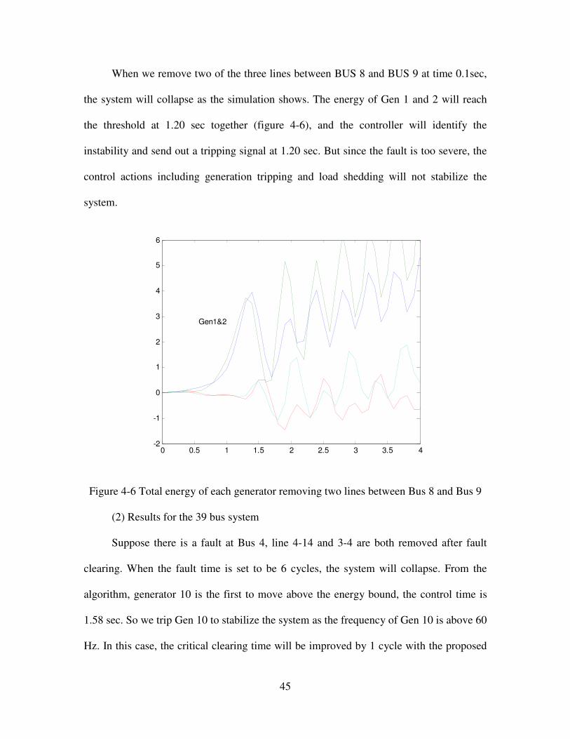
When we remove two of the three lines between BUS 8 and BUS 9 at time 0.1sec,
the system will collapse as the simulation shows. The energy of Gen 1 and 2 will reach
the threshold at 1.20 sec together (figure 4-6), and the controller will identify the
instability and send out a tripping signal at 1.20 sec. But since the fault is too severe, the
control actions including generation tripping and load shedding will not stabilize the
system.
0 0.5 1 1.5 2 2.5 3 3.5 4-2
-1
0
1
2
3
4
5
6
Gen1&2
Figure 4-6 Total energy of each generator removing two lines between Bus 8 and Bus 9
(2) Results for the 39 bus system
Suppose there is a fault at Bus 4, line 4-14 and 3-4 are both removed after fault
clearing. When the fault time is set to be 6 cycles, the system will collapse. From the
algorithm, generator 10 is the first to move above the energy bound, the control time is
1.58 sec. So we trip Gen 10 to stabilize the system as the frequency of Gen 10 is above 60
Hz. In this case, the critical clearing time will be improved by 1 cycle with the proposed
Page 56
46
energy function algorithm.
4.3.2 Consideration of the load level and the load model
(1) Results of the two area system
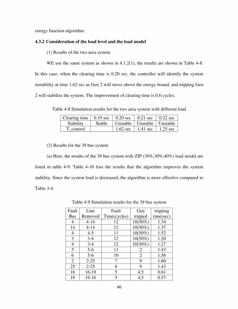
WE use the same system as shown in 4.1.2(1), the results are shown in Table 4-8.
In this case, when the clearing time is 0.20 sec, the controller will identify the system
instability at time 1.62 sec as Gen 2 will move above the energy bound, and tripping Gen
2 will stabilize the system. The improvement of clearing time is 0.6 cycles.
Table 4-8 Simulation results for the two area system with different load
Clearing time 0.19 sec 0.20 sec 0.21 sec 0.22 sec
Stability Stable Unstable Unstable Unstable
T_control 1.62 sec 1.41 sec 1.25 sec
(2) Results for the 39 bus system
(a) Here, the results of the 39 bus system with ZIP (30%,30%,40%) load model are
listed in table 4-9. Table 4-10 lists the results that the algorithm improves the system
stability. Since the system load is decreased, the algorithm is more effective compared to
Table 3-4.
Table 4-9 Simulation results for the 39 bus system
Fault
Bus
Line
Removed
Fault
Time(cycles)
Gen
tripped
tripping
time(sec)
4 4-14 12 10(50%) 1.34
14 4-14 12 10(50%) 1.37
4 4-5 11 10(50%) 1.52
3 3-4 12 10(50%) 1.20
4 3-4 12 10(50%) 1.27
5 5-6 11 2 1.43
6 5-6 10 2 1.56
2 2-25 7 9 1.60
25 2-25 6 9 1.43
16 16-19 5 4,5 0.61
19 19-16 5 4,5 0.57
Page 57
47
21 16-21 10 10(50%) 1.26
16 16-21 8 10(50%) 1.03
Table 4-10 Improvement on the system stability
Fault
Bus
Line
Removed
Fault
Time(cycles)
improvement
4 4-14 3
14 4-14 3
4 4-5 3
3 3-4 2
4 3-4 2
5 5-6 3
6 5-6 2
2 2-25 2
25 2-25 2
16 16-19 0
19 19-16 0
21 16-21 2
16 16-21 2
(b) Continuing with the previous ZIP (30%, 30%, 40%) load model, we increase the
load level to 120% and distribute the load to each generator of the system. Table 4-4
shows the simulation results. The fault time of each fault is the critical time the system
becomes unstable. When the first generator moves above its energy threshold, we take a
generation tripping in accelerating area; at the same time, we also add load shedding
action in decelerating area. In this stressed system, we take the control actions based on
the observation of phase angle measurements with the respect of COA. In each unstable
case, Gen 10 is the one which decelerates from COA, so we shed 50% load (600MW) at
the Bus 39 which is the terminal bus of Gen 10 at the time the first generator moves
beyond threshold. Table 4-11 and Table 4-12 list the simulation results.
Page 58
48
Table 4-11 Simulation results for the 39 bus system in a stress condition
Fault
Bus
Line
Removed
Fault
Time(cycles)
Gen
tripped
tripping
time(sec)
4 4-14 7 2,3 0.98
14 4-14 7 2,3 0.93
4 4-5 6 2,3 1.01
3 3-4 7 2,3 0.99
4 3-4 7 2,3 1.02
5 5-6 6 2 1.10
6 5-6 5 2 1.15
2 2-25 6 9 1.13
25 2-25 5 9 0.98
16 16-19 5 4,5 0.57
19 19-16 5 4,5 0.53
21 16-21 7 2,3 1.03
16 16-21 6 2,3 0.94
Table 4-12 Improvement on the system stability
Fault
Bus
Line
Removed
Fault
Time(cycles)
improvement
4 4-14 0
14 4-14 0
4 4-5 0
3 3-4 1
4 3-4 1
5 5-6 0
6 5-6 0
2 2-25 1
25 2-25 1
16 16-19 0
19 19-16 0
21 16-21 1
16 16-21 1
4.4 COMPARISON AND DISCUSSION
Two new algorithms are proposed with the concept of synchrophasors
measurements in this thesis. The first method uses bus voltage phase angle measurements
to detect the system instability, and the second method is developed with the concept of
Page 59
49
energy function which needs measurements of generator power, mechanical torque, bus
frequency, besides bus voltage phase angle. Therefore, the second algorithm will detect
the system instability more accurately and generally, especially, with the consideration of
frequency.
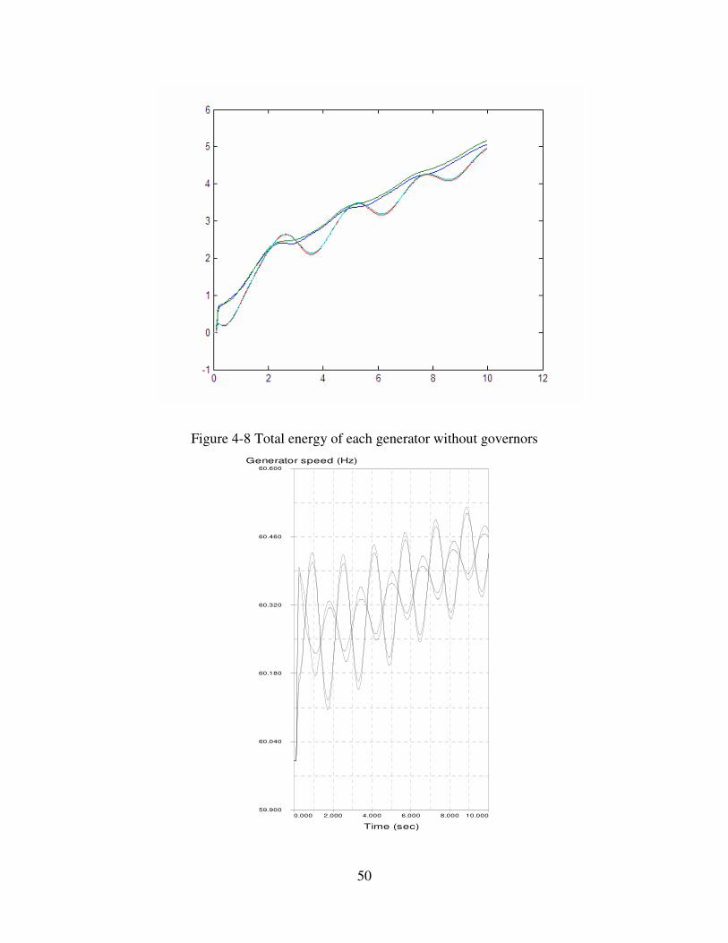
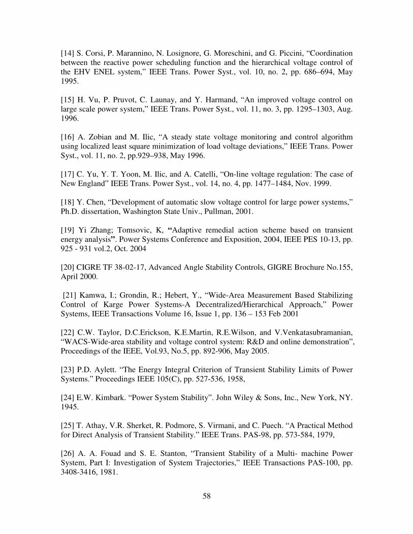
In the two area system, we remove the governors and set up a three phase fault on
Bus 8. Figure 4-7 and Figure 4-8 are the angle and energy of each generator, respectively.
Figure 4-9 gives out the speed of the four generators. For this simple example, using
only phase angle measurements gives out a stable result, while actually the generators are
speeding up. Thus, using energy function can avoid this kind of detecting error.
Figure 4-7 Angles of generators without governors
Page 60
50
Figure 4-8 Total energy of each generator without governors
Generator speed (Hz)
Time (sec)
0.000 2.000 4.000 6.000 8.000 10.00059.900
60.040
60.180
60.320
60.460
60.600
Page 61
51
Figure 4-9 Generator speeds without governors
Considering such a case, in the 39 bus system, suppose a generator tripping at time
0.1 second, the system frequency will drop due to the loss of generation. When we trip
Gen 2 and Gen 4 at time 0.1 second, Figure 4-10 shows the frequency of the generators.
If we use the first algorithm, since the angles will not depart from each other, Figure 4-11
shows the algorithm result. Now, we use the algorithm based on the energy function, the
energy of each generator is shown in Figure 4-12, and Gen 10 will move above the
energy bound at time 2.8 second. Since the system frequency is below 60 Hz, we need to
take the control as load shedding at the Bus near Gen 10. After the load shedding, the
frequency of the generators is shown in Figure 4-13. The discussions above show that the
energy function algorithm takes advantage with the frequency considered.
Generator speed (Hz)
Time (sec)
0.0002.000 4.000 6.000 8.00010.000
57.200
58.540
59.880
61.220
62.560
63.900
Figure 4-10 Frequency of generators when tripping Gen 2 and Gen 4
Page 62
52
0 2 4 6 8 10 12-60
-50
-40
-30
-20
-10
0
10
20
30
Figure 4-11 Angles of generators when tripping Gen 2 and Gen 4
0 0.5 1 1.5 2 2.5 3 3.5 4 4.5 50
50
100
150
10
Figure 4-12 Total energy of each generator when tripping Gen 2 and Gen 4
Page 63
53
Generator speed (Hz)
Time (sec)
0.0002.000 4.000 6.000 8.00010.00059.100
59.280
59.460
59.640
59.820
60.000
Figure 4-13 Frequency of generators after load shedding
Recall Table 2-3 and Table 3-3, comparison is listed in table 4-13. From the table,
we could see that the first algorithm is much faster than the second one, which means it
could save more control time for the system. The integration of the potential energy slows
down the speed of the second algorithm. In the real system, system frequency is well
monitored and controlled with AGC and other devices. Using only phase angle
measurements is easy to implement and fast for detecting the system instability.
Table 4-13 Comparison of two algorithms
Tripping time(sec) Fault
Bus
Line
Removed
Fault
Time(cycles)
Gen
tripped Algorithm1 Algorithm2
4 4-14 13 10 0.76 1.09
14 4-14 13 10 0.78 1.13
4 4-5 12 10 0.88 1.31
3 3-4 12 10 0.73 0.99
4 3-4 11 10 0.84 1.03
5 5-6 11 2 0.90 1.23
Page 64
54
6 5-6 10 2 1.11 1.37
2 2-25 7 9 1.06 1.41
25 2-25 6 9 0.92 1.32
16 16-19 5 4,5 0.52 0.58
19 19-16 5 4,5 0.46 0.52
21 16-21 9 10 0.90 1.02
16 16-21 7 10 0.77 0.92
.
4.5 CONCLUSION
Different simulation conditions are discussed in this chapter. The two algorithms
are compared in the test system. The simple, fast and stable algorithm using bus voltage
phase angle measurements appears to show advantages over the energy function method.
Page 65
55
CHAPTER 5 CONCLUSION
This thesis presents algorithms for processing of phase angle measurements from
across the system to decide whether any part or any control area within the system is
speeding away from the rest. When the angle separations go above preset thresholds,
remedial actions such as generation and load tripping are ordered by the stability
controller to keep the areas in synchronism. This algorithm is meant to be a safety net
when the normal RAS or SPS schemes have failed to operate for whatever reason and
when the system is beginning to separate into islands. The proposed algorithm and the
controller detect the fast separation of phase angles among the critical areas automatically
using the synchrophasors and proceed to mitigate the instability by suitable switching
actions. The thesis tests the new algorithm with illustrative examples on standard IEEE
test systems.
This thesis also proposes the algorithm using real-time computation of energy
functions to detect the system instability. When the system has large transient behaviors,
the energy of the critical generators will move above their energy bound. This algorithm
detects the critical generator’s energy and leads to some witching controls. The energy
function algorithm is also tested on standard IEEE test systems.
Different simulation conditions are discussed in this thesis and the two new
algorithms are compared. The simple, fast and stable algorithm using bus voltage phase
angle measurements takes advantage.
This thesis proposes the algorithm which could detect the system instability and
send out proper control actions. But how much the amounts of the tripping generation or
load shedding should be still needs to be further analyzed in future work. The
Page 66
56
computation and set-up of the thresholds of both algorithms are also need accurate
analysis in real-time system.
Page 67
57
REFERENCES
[1] C. Taylor, D. Erickson, B. Wilson, and K. Martin. (2002, December 16). Wide-Area
Stability and Voltage Control System (WACS) Demonstration.
[2] U.S.–Canada Power System Outage Task Force, “Causes of the August 14th
Blackout
in the United States and Canada,” Interim Rep., Nov. 2003, Ch 6.
[3] “Final report on the August 14, 2003 blackout in the United States and Canada:
Causes and recommendations,” US–Canada Power System Outage Task Force, 2004.
[4] C. W. Taylor and D. C. Erickson, “Recording and analyzing the July 2 cascading
outage,” IEEE Computer Applications in Power, pp. 26-30, vol. 10, January 1997.
[5] P. Kundur, Power System stability and control, McGraw-Hill, 1994
[6] C. W. Taylor, Power system Voltage Stability, McGraw-Hill, 1994
[7] K. Tomsovic, D. Bakken, V. Venkatasubramanian, A. Bose, “Designing the Next
Generation of Real-Time Control, Communication and Computations for Large Power
Systems,” IEEE Proc. – Special Issue on Energy Infrastructure Systems, Proceedings of
IEEE, vol. 93, no. 5, May 2005.
[8] C. Rehtanz, J. Bertsch, “Wide Area Measurement and Protection System for
Emergency Voltage Stability Control,”Power Engineering Society Winter Meeting, 2002.
IEEE, vol. 2, pp. 842 – 847, Jan 2002.
[9] Taylor, C.W., “The Future in On-Line Security Assessment and Wide-Area Stability
control,” Power Engineering Society Winter Meeting, 2000. IEEE, vol. 1, pp. 78 - 83 Jan
2000.
[10] E. Nobile, A. Bose, and K. Tomsovic, “Feasibility of a bilateral market for load
following,” IEEE Trans. Power System., vol. 16, no.4, pp. 782–787, Nov 2001.
[11] X. Yu and K. Tomsovic, “Application of linear matrix inequalities for load
frequency control with communication delays,” IEEE Trans. Power System, vol. 19, no.
3, pp. 1508–1515, Aug 2004.
[12] S. Bhowmik, K. Tomsovic, and A. Bose, “Communication models for third party
load frequency control,” IEEE Trans. Power System, vol.19, no. 1, pp. 543–548, Feb
2004.
[13] J. P. Paul, J. T. Leost, and J. M. Tesseron, “Survey of the secondary voltage control
in France: Present realization and investigations,” IEEE Trans. Power System, vol.
PWRS-2, no. 2, pp. 505–511, May 1987.
Page 68
58
[14] S. Corsi, P. Marannino, N. Losignore, G. Moreschini, and G. Piccini, “Coordination
between the reactive power scheduling function and the hierarchical voltage control of
the EHV ENEL system,” IEEE Trans. Power Syst., vol. 10, no. 2, pp. 686–694, May
1995.
[15] H. Vu, P. Pruvot, C. Launay, and Y. Harmand, “An improved voltage control on
large scale power system,” IEEE Trans. Power Syst., vol. 11, no. 3, pp. 1295–1303, Aug.
1996.
[16] A. Zobian and M. Ilic, “A steady state voltage monitoring and control algorithm
using localized least square minimization of load voltage deviations,” IEEE Trans. Power
Syst., vol. 11, no. 2, pp.929–938, May 1996.
[17] C. Yu, Y. T. Yoon, M. Ilic, and A. Catelli, “On-line voltage regulation: The case of
New England” IEEE Trans. Power Syst., vol. 14, no. 4, pp. 1477–1484, Nov. 1999.
[18] Y. Chen, “Development of automatic slow voltage control for large power systems,”
Ph.D. dissertation, Washington State Univ., Pullman, 2001.
[19] Yi Zhang; Tomsovic, K, “Adaptive remedial action scheme based on transient
energy analysis”. Power Systems Conference and Exposition, 2004, IEEE PES 10-13, pp.
925 - 931 vol.2, Oct. 2004
[20] CIGRE TF 38-02-17, Advanced Angle Stability Controls, GIGRE Brochure No.155,
April 2000.
[21] Kamwa, I.; Grondin, R.; Hebert, Y., “Wide-Area Measurement Based Stabilizing
Control of Karge Power Systems-A Decentralized/Hierarchical Approach,” Power
Systems, IEEE Transactions Volume 16, Issue 1, pp. 136 – 153 Feb 2001
[22] C.W. Taylor, D.C.Erickson, K.E.Martin, R.E.Wilson, and V.Venkatasubramanian,
“WACS-Wide-area stability and voltage control system: R&D and online demonstration”,
Proceedings of the IEEE, Vol.93, No.5, pp. 892-906, May 2005.
[23] P.D. Aylett. “The Energy Integral Criterion of Transient Stability Limits of Power
Systems.” Proceedings IEEE 105(C), pp. 527-536, 1958,
[24] E.W. Kimbark. “Power System Stability”. John Wiley & Sons, Inc., New York, NY.
1945.
[25] T. Athay, V.R. Sherket, R. Podmore, S. Virmani, and C. Puech. “A Practical Method
for Direct Analysis of Transient Stability.” IEEE Trans. PAS-98, pp. 573-584, 1979,
[26] A. A. Fouad and S. E. Stanton, “Transient Stability of a Multi- machine Power
System, Part I: Investigation of System Trajectories,” IEEE Transactions PAS-100, pp.
3408-3416, 1981.
Page 69
59
[27] A. A. Fouad and S. E. Stanton, “Transient Stability of a Multi- machine Power
System, Part 11: Critical Transient Energy,” IEEE Transactions PAS-100, pp. 3417-3424,
1981.
[28] Michel, A. Fouad, A. Vittal, V., “Power system transient stability using individual
machine energy functions”, Circuits and Systems, IEEE Transactions on Volume
30, Issue 5, pp. 266 – 276, May 1983.
[29] S. E. Stanton, “Transient Stability Monitoring for Electric Power Systems Using
Partial Energy Functions,” IEEE Transactions on Power Systems, Vol. 4, No. 4, pp.
1389-1395, 1989.
[30] S. E. Stanton and W. P. Dykas, “Analysis of a Local Transient Control Action by
Partial Energy Functions,” IEEE Transactions on Power Systems, Vol. 4, No. 3, pp. 996-
1002, 1989.
[31] A. A. Fouad and V. Vittal. “Power system Transient Stability Analysis Using the
Transient Energy Function Method”. Prentice Hall, Inc., 1992.
[32] Stanton, S.E., Slivinsky, C., Martin, K., Nordstrom, J., “Application of phasor
easurements and partial energy analysis in stabilizing large disturbances”, Power Systems,
IEEE Transactions on Volume 10, Issue 1, pp. 297 – 306, Feb 1995.
[33] Joe H. Chow, Aranya Chakrabortty, Murat Arcak, Bharat Bhargava, and Armando
Salazar, “Synchronized Phasor Data Based Energy Function Analysis of Dominant Power
Transfer Paths in Large Power Systems”, IEEE Summer Power Meeting, Montreal,
Canada, June 2006.
Page 70
60
APPENDIX
Appendix A Diagram of the two area System
Page 71
61
Appendix B Diagram of the 39 bus System