A2 M4 PowerPoint Part 1 121022.ppt - mpsaz.org · Quadratic functions have the characteristic that...

12/10/2012

1

2

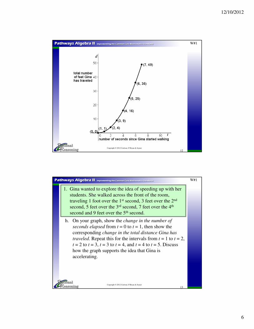
1. Gina wanted to explore the idea of speeding up with her

students. She walked across the front of the room,

traveling 1 foot over the 1st second, 3 feet over the 2nd

second, 5 feet over the 3rd second, 7 feet over the 4th

second and 9 feet over the 5th second.

W#1

INTRODUCTION TO QUADRATIC FUNCTIONS

a. Complete the table to show how far Gina traveled over

each of the following intervals.

IntervalDistance Gina travels

during the interval (feet)

from 0 to 1 second

from 1 to 2 seconds

from 2 to 3 seconds

from 3 to 4 seconds

from 4 to 5 secondsCopyright © 2012 Carlson, O’Bryan & Joyner

3






W#1

INTRODUCTION TO QUADRATIC FUNCTIONS

a. Complete the table to show how far Gina traveled over

each of the following intervals.

IntervalDistance Gina travels

during the interval (feet)

from 0 to 1 second 1

from 1 to 2 seconds 3



from 4 to 5 seconds 9Copyright © 2012 Carlson, O’Bryan & Joyner

12/10/2012

2

4






W#1

b. Do you notice a pattern to how Gina’s distance traveled

over each interval changes? If so, describe the pattern in

your own words.

Over each 1-second interval she traveled 2 feet further than

she did during the previous 1-second interval.

Copyright © 2012 Carlson, O’Bryan & Joyner

5

W#1

c. Explain how you know that Gina’s speed is increasing

(called acceleration).

She travels a greater distance over equal intervals of time as

the time since she began walking increases, so her speed

must be increasing.

d. If Gina continues the same pattern of acceleration, how

far will she travel over the next two 1-second intervals?

She will travel 11 feet from 5 to 6 seconds since she began

walking, and she will travel 13 feet from 6 to 7 seconds

since she began walking.







12/10/2012

3

6

W#1

e. Construct a table of the total distance Gina traveled d

(measured in feet) in terms of the amount of time t

(measured in seconds) since she started walking.

(Assume that Gina stops walking after 7seconds.)







7

W#1

Number of seconds

since Gina began

walking (t)

Total distance

(in feet) Gina

has traveled (d)

Distance Gina

travels during

the interval (∆d)

0

1

13

2

5

37

49

5

6

7


12/10/2012

4

8

W#1

Number of seconds

since Gina began

walking (t)

Total distance

(in feet) Gina

has traveled (d)

Distance Gina

travels during

the interval (∆d)

0 0

1

1 1

3

2 4

5

3 9

7

4 16

95 25

11

6 3613

7 49


9

W#1

Number of seconds

since Gina began

walking (t)

Total distance

(in feet) Gina

has traveled (d)

Distance Gina

travels during

the interval (∆d)

Change

in ∆d

0 0

1

1 13

2 4

5

3 97

4 169

5 2511

6 3613

7 49


12/10/2012

5

10

W#1

Number of seconds

since Gina began

walking (t)

Total distance

(in feet) Gina

has traveled (d)

Distance Gina

travels during

the interval (∆d)

Change

in ∆d

0 0

1

1 1 2

3

2 4 2

5

3 9 2

7

4 16 2

95 25 2

11

6 36 213

7 49


11

W#1

f. How are the number of seconds since Gina began

walking (t) and total distance Gina has traveled (d)

related for integer values of t? Give the formula for d in

terms of t.






The total distance Gina has traveled since she began walking

is the square of the number of seconds she has been walking.

d = t2

g. Construct a graph of Gina’s total distance traveled (in

feet) in terms of the number of seconds since she started

walking for integer values of t. Pay attention to the

domain and range based on the context.Copyright © 2012 Carlson, O’Bryan & Joyner

12/10/2012

6

12

W#1


13

W#1

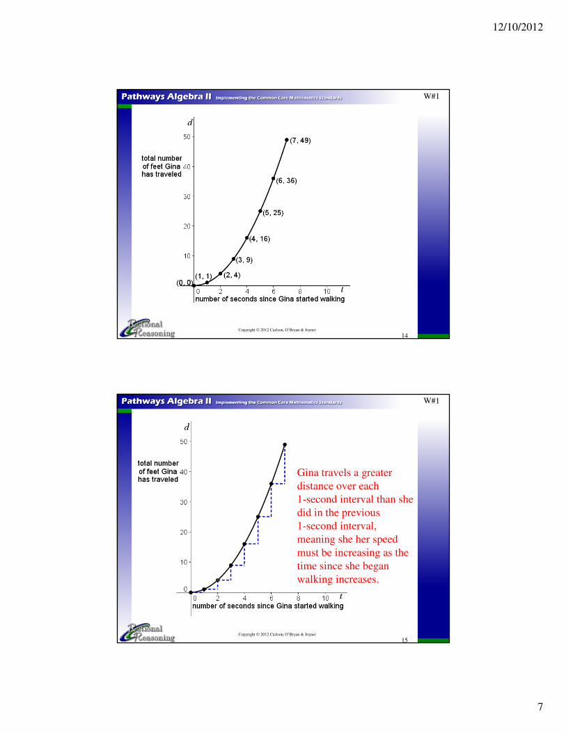
h. On your graph, show the change in the number of

seconds elapsed from t = 0 to t = 1, then show the

corresponding change in the total distance Gina has

traveled. Repeat this for the intervals from t = 1 to t = 2,

t = 2 to t = 3, t = 3 to t = 4, and t = 4 to t = 5. Discuss

how the graph supports the idea that Gina is

accelerating.







12/10/2012

7

14

W#1


15

W#1

Gina travels a greater

distance over each

1-second interval than she

did in the previous

1-second interval,

meaning she her speed

must be increasing as the

time since she began

walking increases.


12/10/2012

8

16

W#1

i. Use the formula you developed in part (f) to fill in the

tables below showing the total distance Gina had traveled

for non-integer values of t.

Number of

seconds since

Gina began

walking (t)

Total distance

(in feet) Gina

has traveled (d)

Number of

seconds since

Gina began

walking (t)

Total distance

(in feet) Gina

has traveled (d)

0 0 0 0

0.5 0.25

1 1 0.5

1.5 0.75

2 4 1 1

2.5 1.25

3 9 1.5

3.5 1.75


Number of

seconds since

Gina began

walking (t)

Total distance

(in feet) Gina

has traveled (d)

Number of

seconds since

Gina began

walking (t)

Total distance

(in feet) Gina

has traveled (d)

0 0 0 0

0.5 0.25 0.25 0.0625

1 1 0.5 0.25

1.5 2.25 0.75 0.5625

2 4 1 1

2.5 6.25 1.25 1.5625

3 9 1.5 2.25

3.5 12.25 1.75 3.0625

17

W#1

j. Calculate Gina’s change in distance over each ½-second

interval (for the table on the left) and each ¼-second

interval (for the table on the right), then determine how

∆d is changing. What pattern do you notice in how Gina’s

distance increases for equal increases in time since she

started walking?


12/10/2012

9

18

W#1

Number of

seconds since

Gina began

walking (t)

Total distance

(in feet) Gina

has traveled (d)

∆dChange in

∆d

0 0

0.5 0.25

1 1

1.5 2.25

2 4

2.5 6.25

3 9

3.5 12.25


Number of

seconds since

Gina began

walking (t)

Total distance

(in feet) Gina

has traveled (d)

∆dChange in

∆d

0 0

0.250.5 0.25

0.75

1 11.25

1.5 2.25

1.75

2 42.25

2.5 6.252.75

3 93.25

3.5 12.25

Number of

seconds since

Gina began

walking (t)

Total distance

(in feet) Gina

has traveled (d)

∆dChange in

∆d

0 0

0.250.5 0.25 0.50

0.75

1 1 0.501.25

1.5 2.25 0.50

1.75

2 4 0.502.25

2.5 6.25 0.50

2.753 9 0.50

3.25

3.5 12.25

19

W#1

Number of

seconds since

Gina began

walking (t)

Total distance

(in feet) Gina

has traveled (d)

∆dChange in

∆d

0 0

0.25 0.0625

0.5 0.25

0.75 0.5625

1 1

1.25 1.5625

1.5 2.25

1.75 3.0625


Number of

seconds since

Gina began

walking (t)

Total distance

(in feet) Gina

has traveled (d)

∆dChange in

∆d

0 0

0.0625

0.25 0.0625

0.1875

0.5 0.250.3125

0.75 0.5625

0.43751 1

0.5625

1.25 1.56250.6875

1.5 2.25

0.8125

1.75 3.0625

Number of

seconds since

Gina began

walking (t)

Total distance

(in feet) Gina

has traveled (d)

∆dChange in

∆d

0 0

0.0625

0.25 0.0625 0.125

0.1875

0.5 0.25 0.1250.3125

0.75 0.5625 0.125

0.43751 1 0.125

0.5625

1.25 1.5625 0.125

0.68751.5 2.25 0.125

0.8125

1.75 3.0625

12/10/2012

10

20

W#1

The function in Exercise #1 is an example of a quadratic

function. Quadratic functions have the characteristic that the

change in the output values follows a linear pattern for equal

changes in the input. The example in Exercise #1 (d = t2) is

the simplest case of a quadratic function. In this case, when

∆t = 1, then ∆d increases by 2 additional feet each second.


21

W#1

Number of

seconds since

Gina began

walking (t)

Total distance

(in feet) Gina

has traveled (d)

Change in the

total distance

Gina has

traveled (∆d)

Change in

∆d

0 0

1 1

2 4

3 9

4 16

5 25

6 36

7 49


Number of

seconds since

Gina began

walking (t)

Total distance

(in feet) Gina

has traveled (d)

Change in the

total distance

Gina has

traveled (∆d)

Change in

∆d

0 0

1

1 1

3

2 45

3 97

4 169

5 2511

6 36

13

7 49

Number of

seconds since

Gina began

walking (t)

Total distance

(in feet) Gina

has traveled (d)

Change in the

total distance

Gina has

traveled (∆d)

Change in

∆d

0 0

1

1 1 2

3

2 4 25

3 9 2

74 16 2

9

5 25 2

116 36 2

13

7 49

12/10/2012

11

22

W#1


23

W#1

x y ∆y Change in ∆y

0 3

2 5

4 11

6 21

8 35

10 53

12 75

14 101


Another example of a quadratic function is shown below. In

this case, when ∆x = 2 we see that ∆y increases by 4 more for

each 2-unit change in x.


0 3

22 5

64 11

106 21

148 35

1810 53

2212 75

2614 101


0 3

22 5 4

64 11 4

106 21 4

148 35 4

1810 53 4

2212 75 4

2614 101

12/10/2012

12

24

W#1


0 –2

2 4

4 10

6 16

8 22

10 28

12 34

14 40


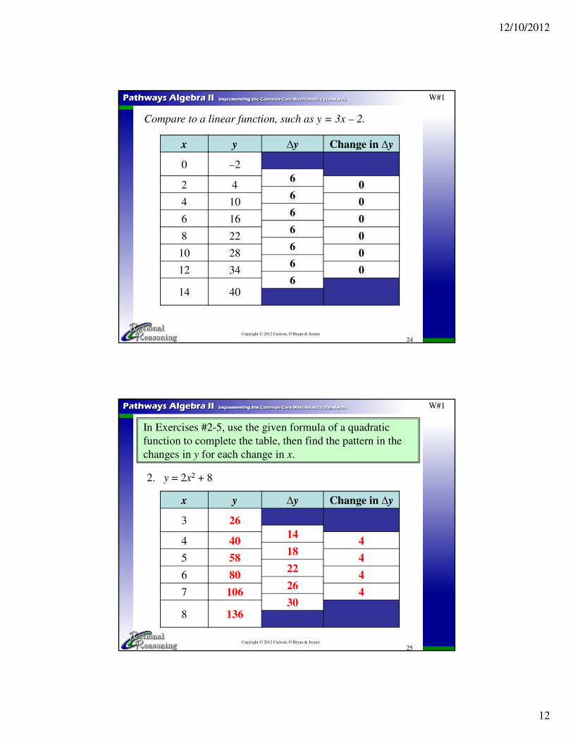
Compare to a linear function, such as y = 3x – 2.


0 –2

62 4

64 10

66 16

68 22

610 28

612 34

614 40


0 –2

62 4 0

64 10 0

66 16 0

68 22 0

610 28 0

612 34 0

614 40

25

W#1

2. y = 2x2 + 8

In Exercises #2-5, use the given formula of a quadratic

function to complete the table, then find the pattern in the

changes in y for each change in x.



3

4

5

6

7

8


3 26

144 40 4

185 58 4

226 80 4

267 106 4

308 136

12/10/2012

13

26

W#1

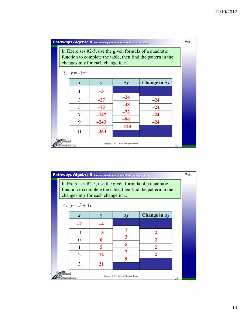
3. y = –3x2






1

3

5

7

9

11


1 –3

–243 –27 –24

–485 –75 –24

–727 –147 –24

–969 –243 –24

–12011 –363

27

W#1

4. y = x2 + 4x






–2

–1

0

1

2

3


–2 –4

1–1 –3 2

30 0 2

51 5 2

72 12 2

93 21

12/10/2012

14

28

W#1

5. y = 2(x + 4)2






–11

–8

–5

–2

1

4


–11 98

–66–8 32 36

–30–5 2 36

6–2 8 36

421 50 36

784 128

29

W#1

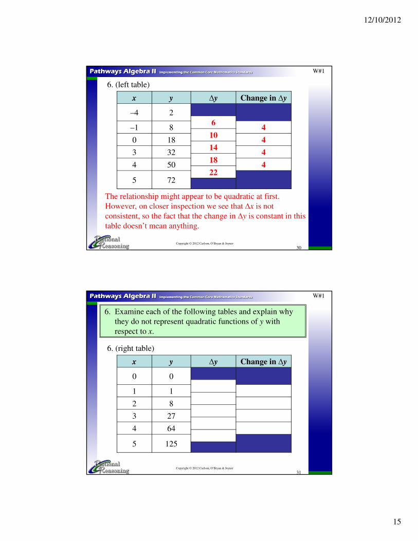
6. (left table)

6. Examine each of the following tables and explain why

they do not represent quadratic functions of y with

respect to x.



–4 2

–1 8

0 18

3 32

4 50

5 72

12/10/2012

15

30

W#1

6. (left table)



–4 2

6–1 8 4

100 18 4

143 32 4

184 50 4

225 72

The relationship might appear to be quadratic at first.

However, on closer inspection we see that ∆x is not

consistent, so the fact that the change in ∆y is constant in this

table doesn’t mean anything.

31

W#1

6. (right table)

6. Examine each of the following tables and explain why

they do not represent quadratic functions of y with

respect to x.



0 0

1 1

2 8

3 27

4 64

5 125

12/10/2012

16

32

W#1

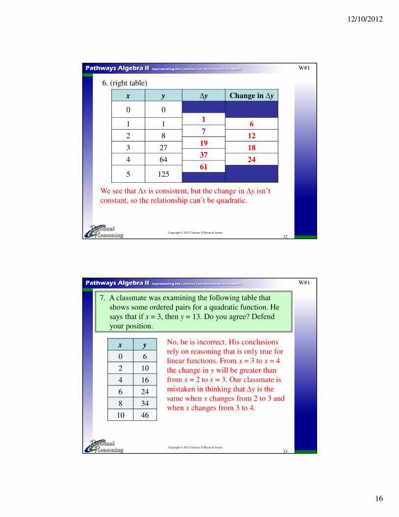
6. (right table)



0 0

11 1 6

72 8 12

193 27 18

374 64 24

615 125

We see that ∆x is consistent, but the change in ∆y isn’t

constant, so the relationship can’t be quadratic.

33

W#1

No, he is incorrect. His conclusions

rely on reasoning that is only true for

linear functions. From x = 3 to x = 4

the change in y will be greater than

from x = 2 to x = 3. Our classmate is

mistaken in thinking that ∆y is the

same when x changes from 2 to 3 and

when x changes from 3 to 4.

7. A classmate was examining the following table that

shows some ordered pairs for a quadratic function. He

says that if x = 3, then y = 13. Do you agree? Defend

your position.


x y

0 6

2 10

4 16

6 24

8 34

10 46

12/10/2012

17

34

W#1

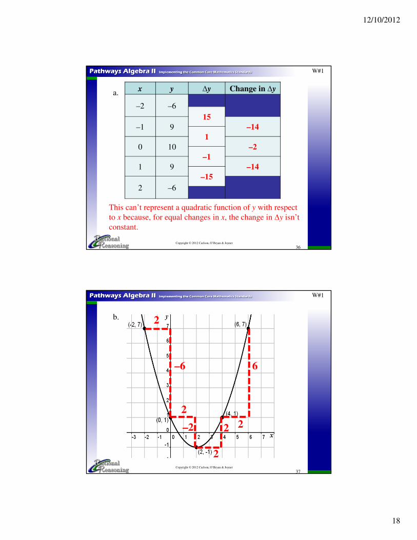
8. The graph of a quadratic function is called a parabola.

Examine the patterns of change of the output while

considering equal increments of change of the input for

each of the following graphs. Which, if any, could

represent the graph of a quadratic function?


a.

35

W#1


a. –11

–15

1

15

11

1

12/10/2012

18

36

W#1


a.x y ∆y Change in ∆y

–2 –6

15

–1 9 –14

1

0 10 –2

–1

1 9 –14

–15

2 –6

This can’t represent a quadratic function of y with respect

to x because, for equal changes in x, the change in ∆y isn’t

constant.

37

W#1


b.

–2

2

–6

2

6

2

2

2

12/10/2012

19

38

W#1



–2 7

–6

0 1 4

–2

2 –1 4

2

4 1 4

6

6 7

This appears to represent a quadratic function of y with

respect to x because, for equal changes in x, the change in

∆y is constant.

b.

39

W#1


c.

–3

–1

–51

1

1

12/10/2012

20

40

W#1



0 –3

–1

1 –4 –2

–3

2 –7 –2

–5

3 –12

This could represent a quadratic function of y with respect

to x because, for equal changes in x, the change in ∆y is

constant. (However, more ordered pairs would allow us to

be more confident.)

c.

41

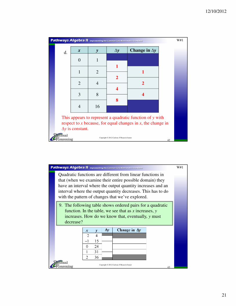
W#1


d.

1

2

1

1

8

1

1

4

12/10/2012

21

42

W#1



0 1

1

1 2 1

2

2 4 2

4

3 8 4

8

4 16

This appears to represent a quadratic function of y with

respect to x because, for equal changes in x, the change in

∆y is constant.

d.

43

W#1

9. The following table shows ordered pairs for a quadratic

function. In the table, we see that as x increases, y

increases. How do we know that, eventually, y must

decrease?


Quadratic functions are different from linear functions in

that (when we examine their entire possible domain) they

have an interval where the output quantity increases and an

interval where the output quantity decreases. This has to do

with the pattern of changes that we’ve explored.

12/10/2012

22

Since ∆y changes by –2 whenever x increases by 1,

eventually ∆y must become negative. When ∆y is negative,

the function is decreasing as x increases.

Let’s continue the table to see this occur.

44Copyright © 2012 Carlson, O’Bryan & Joyner

4

5 –2–1

1

3393

6–3

–2

–2

–2

40

36

39


12/10/2012

23

46

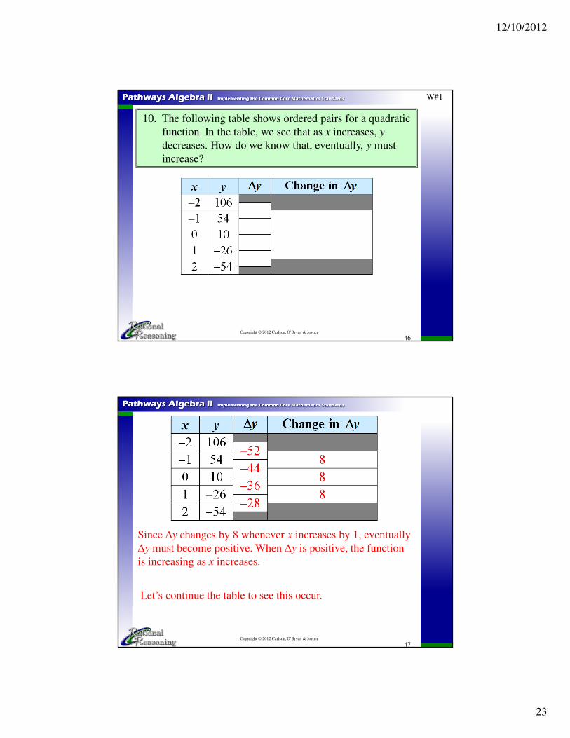
W#1

10. The following table shows ordered pairs for a quadratic

function. In the table, we see that as x increases, y

decreases. How do we know that, eventually, y must

increase?


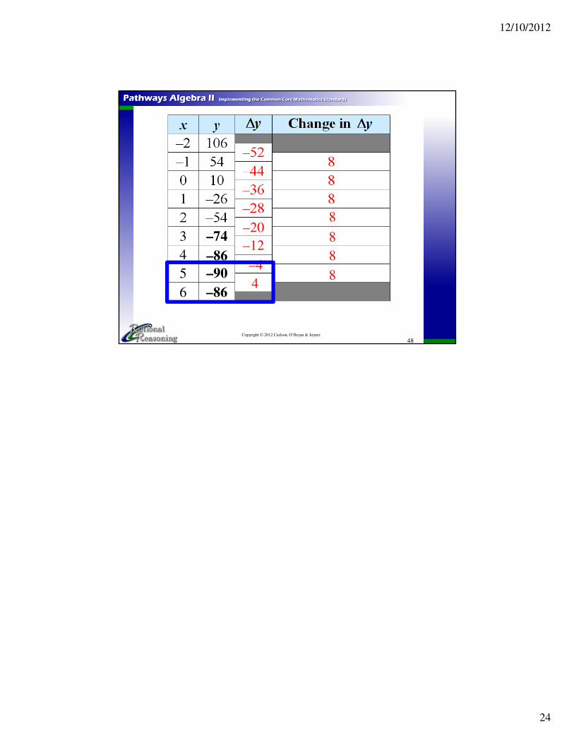
Since ∆y changes by 8 whenever x increases by 1, eventually

∆y must become positive. When ∆y is positive, the function

is increasing as x increases.

Let’s continue the table to see this occur.


12/10/2012

24


4

5 8–4

–12

–20–74 3

64

8

8

8

–86

–86

–90

Date post:	21-Jun-2018
Category:	Documents
Upload:	nguyenxuyen
View:	213 times
Download:	0 times

A2 M4 PowerPoint Part 1 121022.ppt - mpsaz.org · Quadratic functions have the characteristic that...

Documents