Aalborg Universitet Optimization Formulations for the ...

Aalborg Universitet

Optimization Formulations for the Maximum Nonlinear Buckling Load of CompositeStructures

Lindgaard, Esben; Lund, Erik

Published in:Structural and Multidisciplinary Optimization

DOI (link to publication from Publisher):10.1007/s00158-010-0593-8

Publication date:2011

Document VersionAccepted author manuscript, peer reviewed version

Link to publication from Aalborg University

Citation for published version (APA):Lindgaard, E., & Lund, E. (2011). Optimization Formulations for the Maximum Nonlinear Buckling Load ofComposite Structures. Structural and Multidisciplinary Optimization, 43(5), 631-646.https://doi.org/10.1007/s00158-010-0593-8

General rightsCopyright and moral rights for the publications made accessible in the public portal are retained by the authors and/or other copyright ownersand it is a condition of accessing publications that users recognise and abide by the legal requirements associated with these rights.

? Users may download and print one copy of any publication from the public portal for the purpose of private study or research. ? You may not further distribute the material or use it for any profit-making activity or commercial gain ? You may freely distribute the URL identifying the publication in the public portal ?

Take down policyIf you believe that this document breaches copyright please contact us at [email protected] providing details, and we will remove access tothe work immediately and investigate your claim.

https://doi.org/10.1007/s00158-010-0593-8

https://vbn.aau.dk/en/publications/dc3040cf-55ae-43f6-a569-25be9ad0fa85

https://doi.org/10.1007/s00158-010-0593-8

Postprint version, final version available at https://doi.org/10.1007/s00158-010-0593-8

Optimization Formulations for the Maximum Nonlinear Buckl ing Loadof Composite Structures

Esben Lindgaard · Erik Lund

Abstract This paper focuses on criterion functions for gra-dient based optimization of the buckling load of laminatedcomposite structures considering different types of bucklingbehaviour. A local criterion is developed, and is, togetherwith a range of local and global criterion functions from lit-erature, benchmarked on a number of numerical examplesof laminated composite structures for the maximization ofthe buckling load considering fiber angle design variables.The optimization formulations are based on either linear orgeometrically nonlinear analysis and formulated as mathe-matical programming problems solved using gradient basedtechniques. The developed local criterion is formulated suchit captures nonlinear effects upon loading and proves usefulfor both analysis purposes and as a criterion for use in non-linear buckling optimization.

Keywords Composite laminate optimization· Buck-ling · Structural stability· Design sensitivity analysis·Geometrically nonlinear· Composite structures

1 Introduction

Composite materials are mostly used in applications in aerospaceand mechanical industries where their superior stiffness-to-weight or strength-to-weight ratios are critical. Designingstructures made out of composite material represents a chal-lenging task, since both thicknesses, number of plies in thelaminate and their relative orientation must be selected. Thebest use of the capabilities of the material can only be gainedthrough a careful selection of the layup. This may be achieved

Esben Lindgaard (B) · Erik LundDepartment of Mechanical and Manufacturing Engineering,Aalborg University, Aalborg, DenmarkTel.: +45 99407329Fax: +45 98151675E-mail: [email protected]

through a process of design optimization such that the ma-terial properties are tailored to meet particular structural re-quirements with little waste of material capability. A sur-vey of optimal design of laminated plates and shells canbe found in Abrate (1994). This work focuses on optimaldesign of laminated composite shell structures i.e. the opti-mal fiber orientations within the laminate which is a com-plicated problem. Laminated composite shell structures inservice are commonly subjected to various kinds of com-pressive loads which may cause buckling. Hence, structuralinstability becomes a major concern in designing safe andreliable laminated composite shell structures.

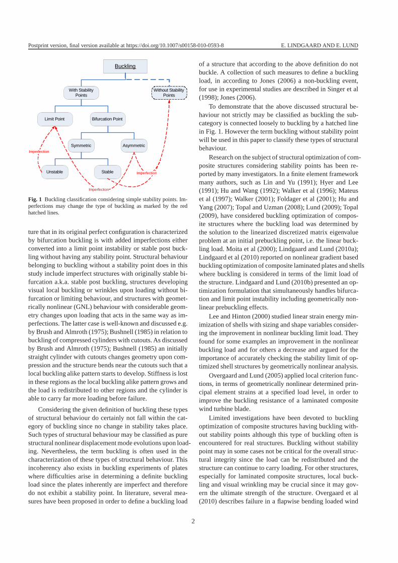
In many works, e.g. Jones (2006), the buckling load istypically defined as the load at which the current equilibriumstate of a structural element or structure suddenly changesfrom a stable to unstable configuration, and is, simultane-ously, the load at which the equilibrium state suddenly changesfrom that previously stable configuration to another stableconfiguration. This may or may not be accompanied withlarge response, i.e. deformation or deflection. The bucklingload is the largest load for which stability of equilibrium ofa structural element or structure exists in its original equi-librium configuration. Considering simple/distinct stabilitypoints this definition of buckling only concerns the part clas-sified as buckling with stability points in Fig. 1. The addi-tional classification of simple stability points, given in Fig. 1,is well-known and printed in many textbooks, such as Thomp-son and Hunt (1973); Jones (2006). For limit point buckling,the buckling load is the load at the limit point and seen as amaximum point in a load-deflection diagram. In case of bi-furcation buckling, the buckling load is the load at the bifur-cation point where another equilibrium path, referred to asthe secondary path, crosses the original/fundamental equi-librium path.

The role of imperfections, i.e. deviations from the per-fect structure which in general can be geometrical, struc-tural, material or load related, is illustrated in Fig. 1. A struc-

Postprint version, final version available at https://doi.org/10.1007/s00158-010-0593-8 E. LINDGAARD AND E. LUND

Buckling

With Stability Points

Without Stability Points

Limit Point Bifurcation Point

Symmetric Asymmetric

Unstable Stable Imperfection

Imperfection

Imperfection

Fig. 1 Buckling classification considering simple stability points. Im-perfections may change the type of buckling as marked by the redhatched lines.

ture that in its original perfect configuration is characterizedby bifurcation buckling is with added imperfections eitherconverted into a limit point instability or stable post buck-ling without having any stability point. Structural behaviourbelonging to buckling without a stability point does in thisstudy include imperfect structures with originally stablebi-furcation a.k.a. stable post buckling, structures developingvisual local buckling or wrinkles upon loading without bi-furcation or limiting behaviour, and structures with geomet-rically nonlinear (GNL) behaviour with considerable geom-etry changes upon loading that acts in the same way as im-perfections. The latter case is well-known and discussed e.g.by Brush and Almroth (1975); Bushnell (1985) in relation tobuckling of compressed cylinders with cutouts. As discussedby Brush and Almroth (1975); Bushnell (1985) an initiallystraight cylinder with cutouts changes geometry upon com-pression and the structure bends near the cutouts such that alocal buckling alike pattern starts to develop. Stiffness is lostin these regions as the local buckling alike pattern grows andthe load is redistributed to other regions and the cylinder isable to carry far more loading before failure.

Considering the given definition of buckling these typesof structural behaviour do certainly not fall within the cat-egory of buckling since no change in stability takes place.Such types of structural behaviour may be classified as purestructural nonlinear displacement mode evolutions upon load-ing. Nevertheless, the term buckling is often used in thecharacterization of these types of structural behaviour. Thisincoherency also exists in buckling experiments of plateswhere difficulties arise in determining a definite bucklingload since the plates inherently are imperfect and thereforedo not exhibit a stability point. In literature, several mea-sures have been proposed in order to define a buckling load

of a structure that according to the above definition do notbuckle. A collection of such measures to define a bucklingload, in according to Jones (2006) a non-buckling event,for use in experimental studies are described in Singer et al(1998); Jones (2006).

To demonstrate that the above discussed structural be-haviour not strictly may be classified as buckling the sub-category is connected loosely to buckling by a hatched linein Fig. 1. However the term buckling without stability pointwill be used in this paper to classify these types of structuralbehaviour.

Research on the subject of structural optimization of com-posite structures considering stability points has been re-ported by many investigators. In a finite element frameworkmany authors, such as Lin and Yu (1991); Hyer and Lee(1991); Hu and Wang (1992); Walker et al (1996); Mateuset al (1997); Walker (2001); Foldager et al (2001); Hu andYang (2007); Topal and Uzman (2008); Lund (2009); Topal(2009), have considered buckling optimization of compos-ite structures where the buckling load was determined bythe solution to the linearized discretized matrix eigenvalueproblem at an initial prebuckling point, i.e. the linear buck-ling load. Moita et al (2000); Lindgaard and Lund (2010a);Lindgaard et al (2010) reported on nonlinear gradient basedbuckling optimization of composite laminated plates and shellswhere buckling is considered in terms of the limit load ofthe structure. Lindgaard and Lund (2010b) presented an op-timization formulation that simultaneously handles bifurca-tion and limit point instability including geometrically non-linear prebuckling effects.

Lee and Hinton (2000) studied linear strain energy min-imization of shells with sizing and shape variables consider-ing the improvement in nonlinear buckling limit load. Theyfound for some examples an improvement in the nonlinearbuckling load and for others a decrease and argued for theimportance of accurately checking the stability limit of op-timized shell structures by geometrically nonlinear analysis.

Overgaard and Lund (2005) applied local criterion func-tions, in terms of geometrically nonlinear determined prin-cipal element strains at a specified load level, in order toimprove the buckling resistance of a laminated compositewind turbine blade.

Limited investigations have been devoted to bucklingoptimization of composite structures having buckling with-out stability points although this type of buckling often isencountered for real structures. Buckling without stabilitypoint may in some cases not be critical for the overall struc-tural integrity since the load can be redistributed and thestructure can continue to carry loading. For other structures,especially for laminated composite structures, local buck-ling and visual wrinkling may be crucial since it may gov-ern the ultimate strength of the structure. Overgaard et al(2010) describes failure in a flapwise bending loaded wind

2


turbine blade, i.e. a large laminated composite structure,asa sequence of failure events where the first is delaminationin the composite laminate triggered by local buckling andsubsequently compressive fibre failure. It could also be pos-tulated that a structure undergoing severe load redistributiondue to the development of a local buckling pattern is un-healthy and operates in a manner, i.e. is carrying loading,that is not intended by the design engineer. Thus, there is alack of optimization formulations that is able to deal withbuckling without stability points. Furthermore, it is unclearhow well the different existing optimization criteria performcompared to one another and to the type of buckling.

This paper deals with the above mentioned problems andbenchmarks a number of objective functions in the attemptto maximize the buckling resistance on a range of differ-ent numerical examples of laminated composite structurescharacterized by different types of buckling. Buckling withstability point of the limit point type and buckling withoutstability point is considered. The already mentioned globaland local buckling criteria from literature are applied in thebenchmark study and a new local criterion is developed andpresented. Linear and geometrically nonlinear analysis isapplied for the different criteria in order to investigate theimportance of including geometrically nonlinear prebuck-ling effects. The developed local criterion is based on geo-metrically nonlinear analysis and formulated such it detectsand captures local nonlinear effects upon loading. It is re-ferred to as the nonlinearity factor criterion. Design sensi-tivities of all buckling criterion functions are obtained semi-analytically by either the direct differentiation approach orby the adjoint approach and the optimization problems areset up as mathematical programming problems solved by agradient based optimization algorithm.

In this work only Continuous Fiber Angle Optimization(CFAO) is considered, thus fiber orientations in laminatelayers with preselected thickness and material are chosen asdesign variables in the laminate optimization. Although fiberangle optimization is known to be associated with a non-convex design space with many local minima it has beenapplied since the laminate parametrization has not been thefocus in this work, i.e. the presented methods in this paperare generic and can easily be used with other parametriza-tions.

The governing equations for linear and nonlinear buck-ling analysis are presented in Sect. 2 together with featuresapplied for buckling detection during geometrically nonlin-ear analysis. The different buckling objective functions ap-plied in the benchmark study are presented in Sect. 3 and theoptimization formulations are stated in Sect. 4. The bench-mark study of the different buckling objective functions areconducted upon a series of numerical examples of laminatedcomposite structures in Sections 5, 6, and 7. Conclusions areoutlined in Sect. 8.

2 Buckling analysis and detection

The finite element method is used for determining the buck-ling load of the laminated composite structure, thus the deriva-tions are given in a finite element context.

A laminated composite is typically composed of multi-ple materials and multiple layers, and the shell structurescanin general be curved or doubly-curved. The materials usedin this work are fiber reinforced polymers, e.g. Glass or Car-bon Fiber Reinforced Polymers (GFRP/CFRP), oriented ata given angleθk for thekth layer. All materials are assumedto behave linearly elastic and the structural behaviour of thelaminate is described using an equivalent single layer the-ory where the layers are assumed to be perfectly bonded to-gether such that displacements and strains will be continu-ous across the thickness.

The solid shell elements used are derived using a contin-uum mechanics approach so the laminate is modelled with ageometric thickness in three dimensions, see Johansen et al(2009). The element used is an eight node isoparametric ele-ment where shear locking and trapezoidal locking is avoidedby using the concepts of assumed natural strains for respec-tively out of plane shear interpolation, see Dvorkin and Bathe(1984), and through the thickness interpolation, see Harnauand Schweizerhof (2002). Membrane and thickness lockingis avoided by using the concepts of enhanced assumed strainfor the interpolation of the membrane and thickness strainsrespectively, see Klinkel et al (1999).

2.1 Linear buckling analysis

Linear buckling analysis is a classical engineering methodfor determining the buckling load of structures. The methodgives numerical inexpensive predictions of buckling withstability point, i.e. singular tangent stiffness. For shell struc-tures it is often used as a generalized stability predictor,asdescribed in Almroth and Brogan (1972), when the stabilitypoint is of bifurcation or even limit point type. Linear buck-ling analysis is based upon linear static analysis where thestatic equilibrium equation for the structure may be writtenas

K0D = R (1)

HereD is the global displacement vector,K0 is the globalinitial stiffness matrix, andR the global load vector.

Based on the displacement field, obtained by the solutionto (1), the element layer stresses can be computed, wherebythe stress stiffening effects due to mechanical loading canbe evaluated by computing the initial stress stiffness matrixKσ. By assuming the structure to be perfect with no geomet-ric imperfections, stresses are proportional to the loads,i.e.stress stiffness depends linearly on the load, displacements

3


at the critical/buckling configuration are small, and the loadis independent of the displacements, the linear buckling prob-lem can be established as

(K0 + λj Kσ)φj = 0, j = 1, 2, . . . , J (2)

where the eigenvalues are ordered by magnitude, such thatλ1 is the lowest eigenvalue, i.e. buckling load factor, andφ1

is the corresponding eigenvector i.e. buckling mode. In gen-eral, for engineering shell structures, the eigenvalue problemin (2) can be difficult to solve, due to the size of the matri-ces involved and large gaps between the distinct eigenvalues.For efficient and robust solutions, (2) is solved by a subspacemethod with automatic shifting strategy, Gram-Schmidt or-thogonalization, and the sub-problem is solved by the Jacobiiterations method, see Wilson and Itoh (1983).

2.2 Nonlinear buckling analysis

Better predictions of structural buckling with stability pointsthan that available by linear buckling analysis may be achievedby nonlinear buckling analysis. The method incorporates ge-ometrically nonlinear analyses and applies for both bifurca-tion and limit point instability, depending on what to appearon the equilibrium path.

Let us consider geometrically nonlinear behaviour of struc-tures made of linear elastic materials. We adopt the TotalLagrangian approach, i.e. displacements refer to the initialconfiguration, for the description of geometric nonlinearity.An incremental formulation is more suitable for nonlinearproblems and it is assumed that the equilibrium at load stepn is known and it is desired at load stepn+1. Furthermore,it is assumed that the current load is independent on defor-mation. The incremental equilibrium equation in the TotalLagrangian formulation is written as (see e.g. Brendel andRamm (1980); Hinton (1992))

KT(Dn, γn) δD = R

n+1 − Fn (3)

KT(Dn, γn) = K0 +KL(D

n, γn) +Kσ(Dn, γn) (4)

KnT= K0 +K

nL+K

nσ

(5)

HereδD is the incremental global displacement vector,Fn

global internal force vector, andRn+1 global applied loadvector. The global tangent stiffnessKn

Tconsists of the global

initial stiffnessK0, the global stress stiffnessKnσ

, and theglobal displacement stiffnessKn

L. The applied load vector

Rn is controlled by the stage control parameter (load fac-

tor) γn according to an applied reference load vectorR

Rn = γn

R (6)

The incremental equilibrium equation (3) is solved by thearc-length method after Crisfield (1981).During the nonlinear path tracing analysis we can at some

converged load step estimate an upcoming critical point, i.e.bifurcation or limit point, by utilizing tangent information.At a critical point the tangent operator is singular

KT(Dc, γc)φj = 0 (7)

where the superscriptc denotes the critical point andφj

the buckling mode. To avoid a direct singularity check ofthe tangent stiffness, it is easier to utilize tangent informa-tion at some converged load stepn and extrapolate it to thecritical point. The one-point approach only utilizes informa-tion at the current step and extrapolates by only one point,see Brendel and Ramm (1980); Borri and Hufendiek (1985).The stress stiffness part of the tangent stiffness at the criticalpoint is approximated by extrapolating the nonlinear stressstiffness from the current configuration as a linear functionof the load factorγ.

Kσ(Dc, γc) ≈ λKσ(D

n, γn) = λKnσ

(8)

It is assumed that the part of the tangent stiffness consist-ing ofKn

LandK0 does not change with additional loading,

which holds if the additional displacements are small. Thetangent stiffness at the critical point is approximated as

KT(Dc, γc) ≈ K0 +K

nL+ λKn

σ(9)

and by inserting into (7) we obtain a generalized eigenvalueproblem

(K0 +KnL)φj = −λjK

nσφj (10)

where the eigenvalues are assumed ordered by magnitudesuch thatλ1 is the lowest eigenvalue andφ1 the correspond-ing eigenvector. The solution to (10) yields the estimate forthe critical load factor at load stepn as

γcj = λjγ

n (11)

If λ1 < 1 the first critical point has been passed and in con-trary λ1 > 1 the critical point is upcoming. The one-pointprocedure works well for both bifurcation and limit points.The closer the current load step gets to the critical point, thebetter the approximation becomes, and it converges to theexact result in the limit of the critical load.

2.3 Buckling detection in GNL analysis

Several different stop criteria are applied for the GNL anal-yses from which an equilibrium point is determined for thedesign sensitivity analysis (DSA) during the optimization,see Table 1. In the case of buckling with a stability pointin the form of a limit point, a limit point detector criterionmay be used. The limit load is simply detected by moni-toring the load factor in the GNL analysis, see (3). Whenthe load factor from two successive load steps decreases the

4


previous converged load is defined as the limit load. A bifur-cation point detector, as described in Lindgaard and Lund(2010b), may be applied in case of bifurcation buckling.For bifurcation point detection nonlinear buckling analysisis performed at precritical stages during GNL analysis as asingularity check on the tangent stiffness. Since bucklingofstructures due to bifurcation is not concerned in the presentpaper this has not been further addressed.

Table 1 Stop criteria applied for buckling detection in GNL analysis.

With stability point

Limit point detectionBifurcation point detection

Without stability point

At load levelAt maximum displacementAt maximum nonlinearity factor,εGNL

In the case of buckling without any stability point otherstop criteria for the GNL analysis are needed. The GNLanalysis may be proceeded towards a certain load level. Eventhough buckling is not detected by this stop criterion it isapplied in the study to investigate the effect of having thechosen equilibrium point for the DSA located closely or faraway from the buckling point. A simple maximum displace-ment criterion monitoring the maximum displacement dur-ing GNL analysis is also applied as a stop criterion for theGNL analysis. Since buckling of a structure typically causesthe displacements to increase disproportionate in compari-son to the load this criterion may be able to detect buck-ling. At last a so-called nonlinearity factor criterion,εGNL,is developed and applied in the study, see (12). The criterionis formulated such it detects local nonlinear effects in thestructural behaviour during loading. Buckling of structuresare in many cases associated with nonlinear effects and ex-tensive load redistribution which has been the motivation forthe developed criterion. The criterion is based on the fractionbetween the principal element strain and the load factor. Therelative change in the fraction from the initial load step1 tothe current load stepn defines the element nonlinearity fac-tor.

εGNL = 1 +

∣

∣

∣

∣

εn1/γn − ε11/γ

1

ε11/γ1

∣

∣

∣

∣

(12)

The nonlinearity factor for linear behaviour isεGNL =1.0 and larger than one when nonlinear behaviour occurs.The stop criterion based on the nonlinearity factor may beactivated for all elements in the numerical model or onlyelements belonging to certain parts of the structure. Notethat all stop criteria described for buckling without stabil-ity points, see Table 1, also may be applied in the case ofbuckling with stability point.

3 Buckling objective functions

A range of different objective functions are investigated andconsidered for the maximum buckling resistance. The ob-jective functions are described in the following and com-ments about the design sensitivity analysis of the differentobjective functions are given. The equations for the designsensitivity analysis are stated in Appendix A.

For the design sensitivities of all objective functions in-volving geometrically nonlinear analyses it is assumed thatthe applied loads are independent of design changes and dis-placements. This is true in the case of laminate optimiza-tion with fiber angle design variables and with conservativeloading, i.e. no follower loads. Furthermore, it is assumedthat the end load level for the design sensitivity analysis isfixed. The latter is not always true since the final load level insome GNL analyses are determined by a GNL stop criterionwhich is not based on a constant load level, see Table 1. Ifconstant load level is not assumed very complicated and nu-merical costly design sensitivity analysis has to be invoked,see Noguchi and Hisada (1993). Applying the fixed load as-sumption the design sensitivity analysis becomes more sim-ple and numerical efficient since the sensitivities can be ob-tained solely by information at the final equilibrium point.Ifthe optimization procedures applying this assumption con-verge towards a constant load level the assumption becomesvalid.

3.1 Linear compliance

Linear complianceCL is defined as the work done by theapplied loads at the equilibrium state expressed in terms ofthe linear static equilibrium equation stated in (1).

CL(D) = RTD (13)

3.2 Nonlinear end compliance

Nonlinear end complianceCGNL is defined as the workdone by the applied loads at the equilibrium state at the finalload stepn expressed in terms of the nonlinear incrementalequilibrium equation stated in (3).

CGNL(Dn,Rn) = (Rn)T

Dn (14)

The expression for the nonlinear end compliance in (14)is in general dependent on both the displacements,D

n andthe external load,Rn at the final load stepn. Consideringdesign changes the nonlinear end compliance criterion ap-plied in this study is only considered dependent upon thedisplacementsDn at the chosen load stepn whereas the ap-plied loadRn is considered independent upon design changes,i.e. CGNL(D

n(a),Rn) where the design variablesai, i =

1, . . . , I, are collected ina.

5


3.3 Nonlinear first principal element strain

An objective function based on the first nonlinear principalelement strain,ε1, is applied in the study since local buck-ling of structures typically is related to large increase indis-placements of certain parts of the structure which eventuallymay result in high strains. Thus, minimizing the elementstrains may prove to be a way of improving the bucklingresistance of a structure. For every converged load stepn

in (3) the element strain tensor may be calculated on basisof the displacement field from which the principal elementstrains can be expressed.

3.4 Element nonlinearity factor

The element nonlinearity factor,εGNL, defined by (12) be-tween an initial load step and the current load step is alsoimplemented as objective function in the study. As explainedearlier, buckling of structures is in many cases associatedwith nonlinear effects and extensive load redistribution.Theelement nonlinearity factor is a local criterion that is devel-oped such it detects nonlinear effects during loading, thusminimizing the element nonlinearity factor may improve thebuckling resistance of a structure.

3.5 Linear buckling

The linear buckling load is obtained as the lowest eigenvalueof (2). Traditionally, the linear buckling load is considered asobjective when the task is to improve the buckling resistanceof structures and therefore applied in the study as a frame ofreference.

3.6 Nonlinear buckling

The nonlinear buckling load is determined at a precriticalload level using the one-point approach by solving the eigen-value problem in (10) and estimating the buckling load bylinear extrapolation in (11). Better predictions of the buck-ling load are generally obtained by nonlinear buckling anal-ysis compared to the traditional linear buckling analysis.Conversely is nonlinear buckling analysis more complicatedand numerical expensive than linear buckling analysis sinceit requires geometrically nonlinear analysis to trace the equi-librium path. The nonlinear buckling load is formulated asan objective function by the procedures originally proposedin Lindgaard and Lund (2010a); Lindgaard et al (2010). Theexpressions for the design sensitivities are as for the otherobjective functions described in Appendix A.

4 Optimization formulations

A range of different optimization formulations is applied inthe study in the attempt to improve the buckling resistanceof a composite structure. The design variables in the numer-ical studies are fiber angles in the laminate layup of a lam-inated composite structure. The optimization problems areall formulated as either a max-min problem or a min-maxproblem. The direct formulation of the optimization prob-lem can give problems related to differentiability and fluctu-ations during the optimization process since, e.g. the eigen-values in the linear buckling problem may change position,i.e. the second lowest eigenvalue can become the lowest. Anelegant solution to this problem is to make use of the so-called bound formulation, see Bendsøe et al (1983); Taylorand Bendsøe (1984); Olhoff (1989). A new artificial vari-ableβ is introduced and a new artificial objective functionβ is chosen. An equivalent problem is formulated, wherethe previous non-differentiable objective function is trans-formed into a set of constraints. Considering a general multiobjective functionFj containingNF function values, themathematical programming problem may be formulated as

Objective: maxa, β

β or mina, β

β

Subject to: Fj ≥ β or Fj ≤ β, j = 1, . . . , NF

ai ≤ ai ≤ ai, i = 1, . . . , I

whereai denote the laminate design variables in terms offiber angles. In case of an objective with many local criterionfunctions, such as min-max nonlinear first principal elementstrain, an active set strategy is employed in order to reducethe number of local criterion functions. Only criterion func-tions with a value larger than70% of the maximum crite-ria function are included in the active set. The mathematicalprogramming problems are solved by the Method of MovingAsymptotes (MMA) by Svanberg (1987). The closed loop ofanalysis, design sensitivity analysis and optimization isre-peated until convergence in the design variables or until themaximum number of allowable iterations has been reached.

The numerical efficiency of the different optimizationformulations depends on the analysis method and the designsensitivity analysis utilized. Please refer to Appendix A fordetails about the design sensitivity analysis. Obviously,lin-ear analysis is more attractive than geometrically nonlinearanalysis in terms of computational cost. The design sensi-tivity analyses of the linear and nonlinear buckling load arecomparable in computational cost but are the most numer-ical demanding of all objective functions considered. Thecomputational cost of the design sensitivity analysis of theelement nonlinearity factor and the nonlinear first principalelement strain are less than the linear and nonlinear buck-

6


ling load but higher than the linear and nonlinear compliancesince the displacement sensitivities need to be computed.

5 Numerical example: laminated composite imperfectplate

The clamped composite laminated plate subjected to a dis-tributed compression load, see Fig. 2, is a structure that hasa stable symmetric point of bifurcation. The bifurcation loadfor the perfect plate estimated by a linear buckling analysisis 438kPa. According to Fig. 1 introductions of imperfec-tions remove the stability point and changes the structuralresponse to a single stable equilibrium path without a stabil-ity point.

Cla

mped. F

ixed in x

, y,

and z

Fixed in z

Dis

trib

ute

d c

om

pre

ssio

n load

y

xz

PSfrag replacements

l

b

l = 5m b = 5m t = 20mmEx = 34GPa Gxy = Gxz = 4.5GPa νxz = 0Gyz = 4.0GPa Ey = Ez = 8.2GPa νxy = νyz = 0.29Initial layup= [90◦/0◦/0◦]s

Fig. 2 Geometry, loads, boundary conditions, and material propertiesfor the laminated composite plate example. The total thickness of theplate is denoted byt and the layup has an equal ply thickness. Thefundamental buckling mode is also shown in contours on the plate.The plate is modelled by400 equivalent single layer solid shell finiteelements.

This characteristic is utilized to construct a simple exam-ple for which buckling appears without any stability points.Geometric imperfections according to the first linear buck-ling mode, see Fig. 2, is superimposed upon the geometrywith a specified amplitude. The amplitude is defined as thelargest translational component of the first linear bucklingmode relative to the thickness of the plate. For this examplean imperfection amplitude of1% has been applied to gener-ate an example that buckles without a stability point. Sincebuckling for the imperfect plate appears without any stabil-ity point the buckling load has to be manually determined

by visual inspection of the equilibrium curve. The equilib-rium path for the initial imperfect plate is shown in Fig. 3.The buckling load is defined when the displacement startsto grow rapidly, i.e. the equilibrium path changes directionfrom the initial part of the path.

A range of different optimization formulations for themaximum buckling resistance is benchmarked upon the ex-ample. The fiber angle in all six fiber layers are used as de-sign variables. An optimization formulation involving non-linear buckling analysis cannot be used since buckling ap-pears without a stability point. Linear buckling optimiza-tion is applied as a frame of reference although no stabil-ity point is present. The optimization formulations bench-marked upon the imperfect composite laminated plate ex-ample are stated in Table 2.

Nine different optimization approaches are applied inthe buckling optimization of the imperfect laminated com-posite plate. Optimization formulation number one and two,see Table 2, applies linear analysis while the others utilizegeometric nonlinear analysis. For the optimizations with ge-ometric nonlinear analysis three different stop criteria havebeen applied to terminate the geometric nonlinear analysis.For e.g. the compliance minimizations, optimization formu-lation number three always complete the GNL analysis tothe same load level, namely a load of550kPa which isslightly above the buckling load of the initial design. Foroptimization formulation four and five the GNL analysis isperformed towards different load levels at each optimiza-tion iteration and controlled by a maximum displacementand a maximum nonlinearity factor criterionεGNL, respec-tively. The threshold values for these stop criteria are setsuch that the reached load level in the GNL analysis is closeto the buckling load. The threshold value for the maximumdisplacementu in x-direction is set to7mm and the maxi-mum nonlinearity factor is set toεGNL = 20. Optimizationformulation number six and seven minimize the maximumfirst principal strains,ε1, whereas optimization formulationeight and nine minimize the maximum nonlinearity factor,εGNL.

The equilibrium curves of the optimized designs accord-ing to the approaches stated in Table 2 are shown in Fig. 3.Almost all optimization approaches lead towards designswith nearly the same equilibrium path and only minor dif-ferences are traceable in the buckling load improvementsshown in Fig. 4.

The laminate designs for all optimization approaches aredriven towards zero degrees fiber angles in all design layers.However for optimization approach four, six, and eight thefiber angle in design layer four for the optimized designsis around60◦ and for optimization approach nine the fiberangle in design layer three and four are−89◦ and104◦, re-spectively.

7


Table 2 Optimization formulations applied in the buckling optimization of the imperfect laminated composite plate.

# Objective function Analysis method Stop criterion

1. Max Min Linear Buckling Linear -2. Min Linear Compliance Linear -3. Min Compliance GNL Load4. Min Compliance GNL Disp.5. Min Compliance GNL εGNL

6. Min Max ε1 GNL Disp.7. Min Max ε1 GNL εGNL

8. Min Max εGNL GNL Disp.9. Min Max εGNL GNL εGNL

0

200

400

600

800

1000

1200

1400

1600

0 10 20 30 40 50

Load [kP

a]

Displacement - u (mm)

Initial Design1. Max Min Linear Buckling

2. Min Linear Compliance3. Min Compliance at Fixed Load (Load = 550kPa)

4. Min Compliance at Updated Load (Disp. = 7mm) 5. Min Compliance at Updated Load (εGNL = 20)

6. Min Max ε1 at Updated Load (Disp. = 7mm)7. Min Max ε1 at Updated Load (εGNL = 20)

8. Min Max εGNL at Updated Load (Disp. = 7mm)9. Min Max εGNL at Updated Load (εGNL = 20)

Fig. 3 Load-deflection curves of the initial laminate composite designand of the optimized designs obtained by the benchmarked optimiza-tion formulations. The displacement is measured at mid spanon theloaded side of the plate and positive in the loading direction.

0

20

40

60

80

100

Buc

klin

g Lo

ad Im

prov

emen

t in

%

9. M

in M

ax ε

GN

L

5. M

in C

ompl

ianc

e

1. M

ax M

in L

inea

r B

uckl

ing

2. M

in L

inea

r C

ompl

ianc

e

3. M

in C

ompl

ianc

e

7. M

in M

ax ε

1

4. M

in C

ompl

ianc

e

8. M

in M

ax ε

GN

L

6. M

in M

ax ε

1

Fig. 4 Buckling load improvement in percent of the imperfect lami-nated composite plate for the benchmarked optimization formulations.

All the benchmarked optimization formulations give sat-isfactory results and are nearly equally good in increasingthe buckling resistance for the imperfect laminated compos-ite plate.

6 Numerical example: laminated composite U-profile

The laminated composite U-profile is an example of a realstructural engineering element. Geometry, loading, and bound-ary conditions are identical to a model analyzed by Klinkelet al (1999); Lindgaard and Lund (2010a); Lindgaard et al(2010). The U-profile is clamped at one end and point loadedin an upper corner node at the other end with a forceR =

250kN . A total of 432 equivalent single layer solid shell fi-nite elements is used in the numerical model.

PSfrag replacements

R

R

w v

L

b

h

t

Geometry:L = 36m

t = {0.05; 0.15}m

b = 2.025m

h = 6.05m

xe

xe

xe

ye

ye

ye

ze ze

ze

Fig. 5 Geometry, loads, boundary conditions, and element coordinatesystems for numerical model of the U-profile.

Two thickness configurations of the U-profile are con-sidered, i.e.t = {0.05; 0.15}m. This leads to two differenttypes of buckling behaviour. The first configuration whichdefines case 1 buckles due to a limit point instability whereascase 2 buckles without any stability point, see e.g. Fig. 1.The laminate layup consists of4 uni-directional E-glass/epoxyfiber layers each of equal thickness, see properties of theprocessed material in Table 3.

The fiber orientation is related to the element coordinatesystem,(xe, ye, ze), in each finite element. The fiber orien-tation is measured counterclockwise from thex-axis in thexy-plane of the element coordinate system. The element co-ordinate system for the finite elements in the web and eachflange, respectively, is depicted in Fig. 5. The fiber orienta-

8


Table 3 Processed material properties for U-profile.

E-glass/epoxyEx 30.6 GPa Ey 8.7 GPaEz 8.7 GPa νxy 0.29νxz 0.3 νyz 0.3Gxy 3.24 GPa Gxz 3.24 GPaGyz 2.9 GPa ρ 1686 kg/m3

tion of each layer for the web and each flange, respectively,is considered constant and the layer stacking is done frominside out. The initial layup definition for the U-profile isstated in Table 4.

Table 4 Layup definition for the U-profile. Each layer in the laminatelayup has equal thickness.

Layup definitionTop Flange (0◦, 45◦,−90◦,−45◦)Web (90◦, 135◦, 0◦, 45◦)Bottom Flange (45◦, 90◦,−45◦, 0◦)

The fiber angles in the layup definition are used as lam-inate design variables in the benchmark study of the differ-ent optimization formulations for maximum buckling resis-tance. Since the U-profile consists of 4 uni-directional fiberlayers at web and each flange this yields a total of 12 designvariables.

6.1 U-profile case 1

Initial analysis of the U-profile with a thickness oft = 0.05mshows buckling of the structure due to a limit point instabil-ity. The linear buckling load and the equilibrium curve froma geometrically nonlinear analysis are depicted in Fig. 6.Linear buckling analysis is unable to predict the limit pointinstability and overestimates the buckling load by27%.

The geometrically nonlinear analysis predicts bucklingdue to a limit point instability where the structure bucklesinthe top flange near the fixed support, see Fig. 7. In contrary,linear buckling analysis predicts bifurcation buckling due tocollapse in the web section at the free end.

The optimization formulations stated in Table 5 are bench-marked upon the U-profile with a thickness oft = 0.05.Since the structure buckles due to a limit point stability,a stability point is present, thus optimization formulationsbased on linear and nonlinear buckling analysis may be ap-plied. Note that the numbering of the optimization formu-lations for this numerical example, see Table 5, is differentfrom that of the previous example, see Table 2.

For the optimization formulations involving geometri-cally nonlinear analysis three different stop criteria have beenapplied to terminate the geometrically nonlinear analysis.

Fig. 6 Linear buckling load and load displacement curve from geo-metrically nonlinear analysis of U-profile.

GNL - At limit p

oint

GNL - Post b

uckling

1lin

ear bucklin

g mode

st

GNL - Post

bucklin

g

PSfrag replacements

R

R

R

R

Fig. 7 1st linear buckling mode shape and displacement field at dif-ferent load steps during the geometrically nonlinear analysis. Note thatthe displacement fields correspond to the marked equilibrium points onthe load displacement curve in Fig. 6.

Those with load based stop criterion continue the GNL anal-ysis until a certain load level is reached. A load of125kNis used in the load based stop criterion. For the optimiza-tion formulations with a stop criterion for the GNL analysisbased on either a limit point detector or a maximum non-linearity factorεGNL, the GNL analysis may be terminatedat different load levels for each optimization iteration. Themaximum nonlinearity factor is set to15 in the stop criterionwhich for the initial laminate design is reached at a load of166kN .

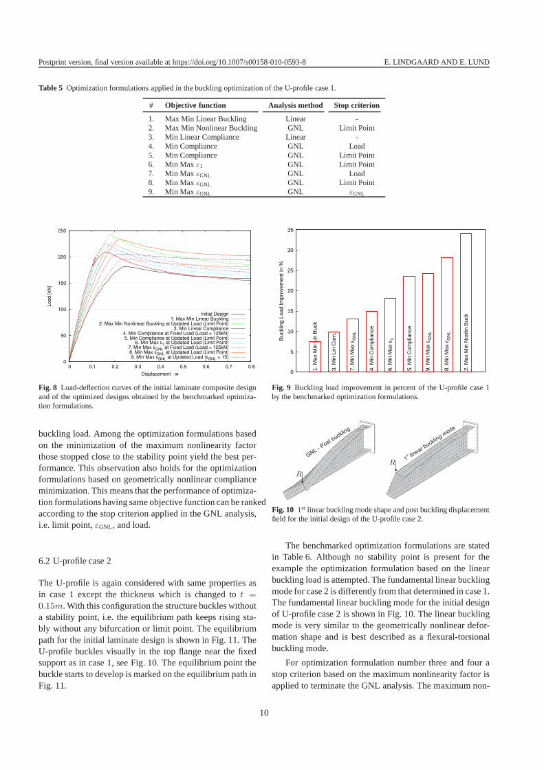
Load-deflection curves of the optimized designs are col-lected in Fig. 8 and the buckling load improvement by thebenchmarked formulations are shown in Fig. 9. All the op-timized designs maintain the same buckling type, i.e. limitpoint instability, and all optimization formulations manageto improve the buckling load.

The poorest performing optimization formulations arethose based on linear analysis, i.e. optimization formula-tion one and three. The best performing optimization for-mulation is number two which is based on the nonlinear

9


Table 5 Optimization formulations applied in the buckling optimization of the U-profile case 1.


1. Max Min Linear Buckling Linear -2. Max Min Nonlinear Buckling GNL Limit Point3. Min Linear Compliance Linear -4. Min Compliance GNL Load5. Min Compliance GNL Limit Point6. Min Max ε1 GNL Limit Point7. Min Max εGNL GNL Load8. Min Max εGNL GNL Limit Point9. Min Max εGNL GNL εGNL

0

50

100

150

200

250

0 0.1 0.2 0.3 0.4 0.5 0.6 0.7 0.8

Load [kN

]

Displacement - w

Initial Design1. Max Min Linear Buckling

2. Max Min Nonlinear Buckling at Updated Load (Limit Point)3. Min Linear Compliance

4. Min Compliance at Fixed Load (Load = 125kN)5. Min Compliance at Updated Load (Limit Point)

6. Min Max ε1 at Updated Load (Limit Point)7. Min Max εGNL at Fixed Load (Load = 125kN)8. Min Max εGNL at Updated Load (Limit Point)9. Min Max εGNL at Updated Load (εGNL = 15)

Fig. 8 Load-deflection curves of the initial laminate composite designand of the optimized designs obtained by the benchmarked optimiza-tion formulations.

buckling load. Among the optimization formulations basedon the minimization of the maximum nonlinearity factorthose stopped close to the stability point yield the best per-formance. This observation also holds for the optimizationformulations based on geometrically nonlinear complianceminimization. This means that the performance of optimiza-tion formulations having same objective function can be rankedaccording to the stop criterion applied in the GNL analysis,i.e. limit point,εGNL, and load.

6.2 U-profile case 2

The U-profile is again considered with same properties asin case 1 except the thickness which is changed tot =

0.15m. With this configuration the structure buckles withouta stability point, i.e. the equilibrium path keeps rising sta-bly without any bifurcation or limit point. The equilibriumpath for the initial laminate design is shown in Fig. 11. TheU-profile buckles visually in the top flange near the fixedsupport as in case 1, see Fig. 10. The equilibrium point thebuckle starts to develop is marked on the equilibrium path inFig. 11.

0

5

10

15

20

25

30

35

Buc

klin

g Lo

ad Im

prov

emen

t in

%

1. M

ax M

in L

in B

uck

3. M

in L

in C

om.

7. M

in M

ax ε

GN

L

4. M

in C

ompl

ianc

e

6. M

in M

ax ε

1

5. M

in C

ompl

ianc

e

9. M

in M

ax ε

GN

L

8. M

in M

ax ε

GN

L

2. M

ax M

in N

onlin

Buc

k

Fig. 9 Buckling load improvement in percent of the U-profile case 1by the benchmarked optimization formulations.

1lin

ear bucklin

g mode

stGNL - Post b

uckling

PSfrag replacements

R

R

Fig. 10 1st linear buckling mode shape and post buckling displacementfield for the initial design of the U-profile case 2.

The benchmarked optimization formulations are statedin Table 6. Although no stability point is present for theexample the optimization formulation based on the linearbuckling load is attempted. The fundamental linear bucklingmode for case 2 is differently from that determined in case 1.The fundamental linear buckling mode for the initial designof U-profile case 2 is shown in Fig. 10. The linear bucklingmode is very similar to the geometrically nonlinear defor-mation shape and is best described as a flexural-torsionalbuckling mode.

For optimization formulation number three and four astop criterion based on the maximum nonlinearity factor isapplied to terminate the GNL analysis. The maximum non-

10


linearity factor is set to100 which for the initial design isreached at a load of1600kN .

The equilibrium curves of the optimized designs obtainedby the benchmarked optimization formulations are collec-tively shown in Fig. 11. The load level at which a bucklestarts to develop in the top flange is marked on the equilib-rium curves and is purely determined by visual inspection ofthe deformation shape. Considering this point as the buck-ling load, the best improvement is obtained by optimizationformulation number four that minimizes the maximum non-linearity factor in the structure. Surprisingly, the second bestdesign is obtained by optimization formulation number onethat maximizes the linear buckling load, despite the absenceof a stability point.

0

500

1000

1500

2000

2500

0 0.5 1 1.5 2 2.5 3

Load (

kN

)

Displacement - w

Initial Design1. Min Lin Buck

2. Min Lin Compliance3. Min Compliance at Updated Load (εGNL = 100)

4. Min Max εGNL at Updated Load (εGNL = 100)Buckling Points

Fig. 11 Load-deflection curves of the initial laminate composite de-sign and of the optimized designs obtained by the benchmarked opti-mization formulations for U-profile case 2.

Using the optimization formulations based on minimumcompliance, i.e. optimization formulation two and three, astability point in the form of a limit point is introduced dur-ing optimization. The compliance minimization based onGNL analysis performs better than the linear compliance op-timized design which again demonstrates the importance ofincluding nonlinear prebuckling displacements.

7 Numerical example: laminated composite box-profile

The laminated composite box-profile depicted in Fig. 12 isclamped at one end and point loaded at the other end. Thebox-profile is divided into five structural parts which consistof two webs and three flanges. A total of1980 equivalentsingle layer solid shell finite elements is used in the numeri-cal model.

The laminate layup consists of4 uni-directional E-glass/epoxyfiber layers, each of equal thickness, for each of the five

PSfrag replacements

RR

L

b

h

t1

t2

t3

Geometry:L = 7mb = 0.5m

h = 1.2m

{t1; t2; t3} = {1; 3; 1.5}10−2m

xe

xe

xe

ye

ye

ye

ze

ze

ze

Fig. 12 Geometry, loads, boundary conditions, and element coordinatesystems for the numerical model of the box-profile.

structural parts in the box-profile, see Table 7. The mate-rial properties of the uni-directional E-glass/epoxy are iden-tical to those used for the U-profile example, see Table 3.The fiber orientation is again related to the element coordi-nate system,(xe, ye, ze), in each finite element and the sameorientational definition of the fiber layers as used for the U-profile is applied. The element coordinate system for the fi-nite elements for the webs and flanges are shown in Fig. 12.The fiber orientation of each layer for each of the five struc-tural parts is considered constant throughout the length ofthe profile and the layer stacking is done in accordance withtheze-axis. The fiber angles in the layup definition are usedas laminate design variables in the benchmark study of theoptimization formulations which gives a total of20 designvariables.

Initial analyses of the box-profile show that the structurebuckles without any loss of stability and without any pointsof stability, i.e. limit point or bifurcation point. The load-deflection curve of the initial design obtained by a geomet-rically nonlinear analysis is depicted in Fig. 15 and defor-mation shapes at different load levels are shown in Fig. 13together with the first linear buckling mode.

PSfrag replacements

R

Fig. 13 1st linear buckling mode shape and displacement field at dif-ferent load steps during the geometrically nonlinear analysis. Note thatthe displacement fields correspond to the marked equilibrium points(80, 127, and195kN) on the load displacement curve in Fig. 15 forthe initial design.

11


Table 6 Optimization formulations applied in the buckling optimization of the U-profile case 2.


1. Max Min Linear Buckling Linear -2. Min Linear Compliance Linear -3. Min Compliance GNL εGNL

4. Min Max εGNL GNL εGNL

Table 7 Layup definition for the box-profile. Each layer in the lami-nate layup has equal thickness.

Layup definitionTop Flange (0◦, 90◦, 90◦, 0◦)Middle Flange (0◦, 90◦, 90◦, 0◦)Bottom Flange (0◦, 90◦, 90◦, 0◦)Right Web (0◦, 90◦, 90◦, 0◦)Left Web (0◦,−90◦,−90◦, 0◦)

At a load level of80kN a visual buckle initiates in thebottom flange and enhances with additional loading and abuckling pattern propagates in the bottom flange in the lengthdirection of the box-profile. The initiation of buckling in thebottom flange results in a stiffness decrease for the struc-ture which immediately may be observed by the change inslope for the load-deflection curve of the initial design, seeFig. 15. The buckling initiation is as already mentioned notconnected to any stability point. This has been verified bysingularity checks upon the tangent stiffness matrix duringGNL analysis, i.e. no singular points could be found.

At buckling, the bottom flange loses its stiffness andthereby its load carrying capability and load redistributionoccurs from the bottom flange to the other structural partsin the box-profile. The load carried by the bottom flange ismainly redistributed to the webs and the middle flange. Themiddle flange is prior to buckling almost unloaded since itlies in the neutral plane. After buckling the position of theneutral plane is shifted so it lies between the top and middleflange, i.e. the middle flange becomes compression loaded.The load redistribution that occurs in connection with theinitiation of buckling in the bottom flange is well capturedby the nonlinearity factor,εGNL, which is plotted in Fig. 14for the four fiber layers at the buckling load of80kN for theinitial design.

The nonlinearity factor,εGNL, is largest for the elementsin the middle flange since those elements initially are al-most unloaded, thus a large change occurs in the principalstrain relative to the load factor. Also the elements in therear end of the bottom flange have nonlinearity factors dif-ferently from1 since the bottom flange buckles and load re-distribution occurs whereby the compressive principal strainrelative to the load factor is reduced.

The optimization formulations stated in Table 8 are bench-marked upon the box-profile in the attempt to maximize the

Design layer 1

1.163E+000

1.151E+000

1.140E+000

1.128E+000

1.116E+000

1.105E+000

1.093E+000

1.081E+000

1.070E+000

1.058E+000

1.047E+000

1.035E+000

1.023E+000

1.012E+000

1.000E+000

Design layer 2

1.754E+000

1.700E+000

1.646E+000

1.592E+000

1.538E+000

1.484E+000

1.431E+000

1.377E+000

1.323E+000

1.269E+000

1.215E+000

1.161E+000

1.108E+000

1.054E+000

1.000E+000

Design layer 3

1.754E+000

1.700E+000

1.646E+000

1.592E+000

1.538E+000

1.484E+000

1.431E+000

1.377E+000

1.323E+000

1.269E+000

1.215E+000

1.161E+000

1.108E+000

1.054E+000

1.000E+000

Design layer 4

1.238E+000

1.221E+000

1.204E+000

1.187E+000

1.170E+000

1.153E+000

1.136E+000

1.119E+000

1.102E+000

1.085E+000

1.068E+000

1.051E+000

1.034E+000

1.017E+000

1.000E+000

Fig. 14 Plots of the nonlinearity factor,εGNL, for all design layers atthe buckling load of the initial laminate design. Note that the box-profile is seen from the rear end.

buckling load. Since the nonlinearity factor is largest fortheelements in the middle flange that are far away from thestructural part that buckles, i.e. the bottom flange, it is at-tempted both to minimize the maximum nonlinearity fac-tor for all elements in the model and to minimize the maxi-mum nonlinearity factor for only the elements in the bottomflange. The optimization that operates on all elements in themodel is referred to as Min Max GlobalεGNL whereas theoptimization that only operates on the elements in the bot-tom flange is referred to as Min Max LocalεGNL. The stopcriterion,εGNL, in the GNL analysis is for local detection setto εGNL = 1.5 and for global detection set toεGNL = 2.9

which both are reached after visual buckling at a load levelclose to the buckling load. The threshold values for the non-linearity factor used in GNL analyses are reached at approx-imately85kN for the initial design which is just above thevisually determined buckling load of80kN .

Although no stability point exists for the box-profile anoptimization that maximizes the minimum linear bucklingload is attempted. This is done since the fundamental lin-ear buckling mode is very similar to the GNL post bucklingdeformation shape, see Fig. 13.

12


Table 8 Optimization formulations applied in the buckling optimization of the box-profile.


1. Max Min Linear Buckling Linear -2. Min Linear Compliance Linear -3. Min Compliance GNL LocalεGNL

4. Min Max GlobalεGNL GNL GlobalεGNL

5. Min Max LocalεGNL GNL Local εGNL

Equilibrium curves of the optimized designs obtained bythe optimization formulations stated in Table 8 are collec-tively shown in Fig. 15.

Fig. 15 Load-deflection curves of the initial laminate composite de-sign and of the optimized designs obtained by the benchmarked opti-mization formulations for the box-profile.

Both optimization formulations based on minimum com-pliance, i.e. linear and GNL, yield almost the same equilib-rium curve and only little improvement in the buckling loadmay be observed. The buckling load is increased by5% and8% by the design based on minimum linear compliance andminimum GNL compliance, respectively. As expected, theoverall stiffness of the structure is increased by the optimiza-tions based on minimum compliance.

Considering the design obtained by the maximum lin-ear buckling load a buckling load improvement of57% isachieved. Thus an optimization formulation based on globalstability as the case for optimization formulation numbertwo, see Table 8, is able to increase the buckling load evenwhen no global stability point is present.

The buckling load improvement by optimization formu-lation number four and five is25% and80%, respectively.Thus optimization formulation five that operates directly uponthe elements in the structural part where the buckle initiatesgives a much better buckling load improvement than the op-timization formulation that operates on the maximum non-linearity factor of all elements within the model. Although

the nonlinearity factors,εGNL, for all elements are highlyaffected by buckling initiation in the bottom flange, not alllocal criterion functions are capable of representing thisre-lation. For the elements in the structural area of instabilitythere is a better correspondance between the local criterionfunctions based on the nonlinearity factor and the bucklinginitiation. This statement is also emphazised by the fact thatthe global level ofεGNL is lower at the buckling point for thelocal εGNL optimized design than for the buckling point forthe globalεGNL optimized design.

8 Conclusions

In this work a range of different criterion functions for themaximum buckling resistance of laminated composite struc-tures is benchmarked upon different numerical examples hav-ing different buckling behaviour. The majority of the crite-rion functions applied in the benchmark study is from liter-ature and concerns both local and global criterion functionsbased on either linear or geometrically nonlinear analysis. Anew local criteria function in terms of an element quantity ispresented and is formulated such it gives a measure for localnonlinear effects upon loading and referred to as the elementnonlinearity factor. The maximum buckling load is obtainedby gradient based optimization and the design sensitivitiesfor all criteria are determined semi-analytically by either thedirect differentiation method or by the adjoint approach.

In the benchmark study buckling with stability point ofthe limit point type and buckling without stability point areconcerned. The latter type may in principle not be classi-fied as buckling since loss of stability does not take place.Though, the term buckling is in many cases used to describee.g. behaviour of imperfect structures with initially stablebifurcation a.k.a. stable post buckling, structures developingvisual local buckling or wrinkles upon loading without bi-furcation or limiting behaviour, and structures with geomet-rically highly nonlinear behaviour with considerably geom-etry changes that act in the same manner as imperfections.

From the benchmark study it is found that different cri-terion functions should be applied depending on the typeof buckling in order to obtain the best buckling load im-provement and thereby the best performing structural de-sign. In general do optimization formulations including non-

13


linear prebuckling effects by geometrically nonlinear analy-sis give better results than those based on linear analysis.

For structures exhibiting a limit point type buckling thecriterion based on the nonlinear buckling load is favoured.This criterion works directly upon the limit point load andthe method includes accurate nonlinear path tracing analysiswhere the buckling load is estimated at a precritical point onthe deformed configuration. The estimation point is alwayschosen close to the real buckling point for a precise estimateof the nonlinear buckling load and the nonlinear bucklingload design sensitivities. Compared to the other criterionfunctions benchmarked, the nonlinear buckling load crite-rion is far superior in the case of limit point buckling.

For cases where buckling alike patterns develop with theabsence of a stability point, i.e. buckling without a stabil-ity point, the local criteria, referred to as the element non-linearity factor, yield the best buckling load improvement.The element measure is able to detect local nonlinear effectsupon loading, in particular load redistribution which oftentakes place with local buckling pattern development. In thenumerical studies it was found that the element nonlinearityfactor in some cases may have values in parts of the struc-ture that are larger than where the buckling pattern propa-gates. For such cases it is better to focus the optimization onthe part of the structure where the buckling pattern initiatesin order to obtain the best buckling load improvement andsuppression of the buckling pattern.

Acknowledgements The authors gratefully acknowledge the supportfrom the Danish Center for Scientific Computing (DCSC) for the hy-brid Linux Cluster “Fyrkat” at Aalborg University, Denmark.

References

Abrate S (1994) Optimal design of laminated plates and shells. Com-pos Struct 29:269–286

Almroth BO, Brogan FA (1972) Bifurcation buckling as an approxima-tion of the collapse load for general shells. AIAA J 10(4):463–467

Bendsøe MP, Sigmund O (2003) Topology optimization - theory, meth-ods and applications, 2nd edn. Springer Verlag Berlin HeidelbergNew York, ISBN: 3-540-42992-1

Bendsøe MP, Olhoff N, Taylor J (1983) A variational formulation formulticriteria structural optimization. J Struct Mech 11:523–544

Borri C, Hufendiek HW (1985) Geometrically nonlinear behaviour ofspace beam structures. J Struct Mech 13:1–26

Brendel B, Ramm E (1980) Linear and nonlinear stability analysis ofcylindrical shells. Compt Struct 12:549–558

Brush DO, Almroth BO (1975) Buckling of bars, plates, and shells.McGraw-Hill Kogakusha, ISBN: 07-085028-3

Bushnell D (1985) Computerized buckling analysis of shells. MartinusNijhoff Publishers, ISBN: 90-247-3099-6

Courant R, Hilbert D (1953) Methods of mathematical physics, vol 1.New York : Interscience Publishers

Crisfield MA (1981) A fast incremental/iterative solution procedurethat handles “snap-through”. Compt Struct 13:55–62

Dvorkin EN, Bathe KJ (1984) A continuum mechanics based four-node shell element for general non-linear analysis. Eng Comput1:77–88

Foldager JP, Hansen JS, Olhoff N (2001) Optimization of the bucklingload for composite structure taking thermal effects into account.Struct Multidiscip Optim 21:14–31

Harnau M, Schweizerhof K (2002) About linear and quadratic “solid-shell” elements at large deformations. Compt Struct 80(9-10):805–817

Hinton E (ed) (1992) NAFEMS Introduction to Nonlinear Finite Ele-ment Analysis. Bell and Bain Ltd, Glasgow, ISBN 1-874376-00-X

Hu HT, Wang SS (1992) Optimization for buckling resistance offiber-composite laminate shells with and without cutouts. ComposStruct 22(2):3–13

Hu HT, Yang JS (2007) Buckling optimization of laminated cylin-drical panels subjected to axial compressive load. Compos Struct81:374–385

Hyer MW, Lee HH (1991) The use of curvilinear fiber format to im-prove buckling resistance of composite plates with centralcircularholes. Compos Struct 18(5/6):239–261

Johansen L, Lund E, Kleist J (2009) Failure optimization of geometri-cally linear/nonlinear laminated composite structures using a two-step hierarchical model adaptivity. Compt Methods Appl MechEngrg 198(30-32):2421–2438

Jones RM (2006) Buckling of bars, plates, and shells. Bull Ridge Pub-lishing, ISBN: 0-9787223-0-2

Klinkel S, Gruttmann F, Wagner W (1999) A continuum based three-dimensional shell element for laminated structures. ComptStruct71 (1):43–62

Lee SJ, Hinton E (2000) Dangers inherited in shells optimized withlinear assumptions. Compt Struct 78:473–486

Lin CC, Yu AJ (1991) Optimum weight design of composite laminatedplates. Compt Struct 38(5/6):581–587

Lindgaard E, Lund E (2010a) Nonlinear buckling optimization ofcomposite structures. Compt Methods Appl Mech Engrg 199(37-40):2319–2330, DOI 10.1016/j.cma.2010.02.005

Lindgaard E, Lund E (2010b) A unified approach to nonlinear bucklingoptimization of composite structures. Submitted

Lindgaard E, Lund E, Rasmussen K (2010) Nonlinear buck-ling optimization of composite structures considering “worst”shape imperfections. Int J Solids Struct 47:3186–3202, DOI10.1016/j.ijsolstr.2010.07.020

Lund E (2009) Buckling topology optimization of laminated multi-material composite shell structures. Compos Struct 91:158–167

Lund E, Stegmann J (2005) On structural optimization of compositeshell structures using a discrete constitutive parametrization. WindEnergy 8:109–124, DOI 10.1002/we.132

Mateus HC, Soares CMM, Soares CAM (1997) Buckling sensitivityanalysis and optimal design of thin laminated structures. ComptStruct 64(1-4):461–472

Moita JS, Barbosa JI, Soares CMM, Soares CAM (2000) Sensitivityanalysis and optimal design of geometrically non-linear laminatedplates and shells. Compt Struct 76:407–420

Noguchi H, Hisada T (1993) Sensitivity analysis in post-buckling prob-lems of shell structures. Compt Struct 47(4/5):699–710

Olhoff N (1989) Multicriterion structural optimization via bound for-mulation and mathematical programming. Struct Optim 1:11–17

Overgaard LCT, Lund E (2005) Structural design sensitivityanalysisand optimization of vestas V52 wind turbine blade. In: Proc.6thWorld Congress on Structural and Multidisciplinary Optimization

Overgaard LCT, Lund E, Thomsen OT (2010) Structural collapseof a wind turbine blade. Part A: Static test and equivalent sin-gle layered models. Composites Part A 41(2):257–270, DOI10.1016/j.compositesa.2009.10.011

Singer J, Arbocz J, Weller T (1998) Buckling experiments: Experi-mental methods in buckling of thin-walled structures, vol 1. JohnWiley & Sons, ISBN: 0-471-95661-9

Svanberg K (1987) Method of moving asymptotes - a new method forstructural optimization. Int J Numer Methods Eng 24:359–373

14


Taylor JE, Bendsøe MP (1984) An interpretation of min-max structuraldesign problems including a method for relaxing constraints. Int JSolids Struct 20(4):301–314

Thompson JMT, Hunt GW (1973) A general theory of elastic stability.John Wiley & Sons, ISBN: 0-471-85991-5

Topal U (2009) Multiobjective optimization of laminated compos-ite cylindrical shells for maximum frequency and buckling load.Mater Des 30:2584–2594

Topal U, Uzman Ü (2008) Maximization of buckling load of laminatedcomposite plates with central circular holes using mfd method.Struct Multidiscip Optim 35:131–139

Walker M (2001) Multiobjective design of laminated plates for max-imum stability using the finite element method. Compos Struct54:389–393

Walker M, Adali S, Verijenko V (1996) Optimization of symmetriclaminates for maximum buckling load including the effects ofbending-twisting coupling. Compt Struct 58(2):313–319

Wilson EL, Itoh T (1983) An eigensolution strategy for largesystems.Compt Struct 16:259–265

Wittrick WH (1962) Rates of change of eigenvalues, with reference tobuckling and vibration problems. J Roy Aeronaut Soc 66:590–591

A Design sensitivity analysis

A.1 Linear displacement sensitivity

The displacement sensitivitiesdDdai

are computed by direct differentia-tion of the static equilibrium equation, see (1), w.r.t. a design variableai, i = 1, . . . , I.

K0

dD

dai= −

dK0

daiD+

dR

dai, i = 1, . . . , I (15)

The displacement sensitivitydDdai

can be evaluated by backsubstitutionof the factored global initial stiffness matrix in (15). Theinitial stiff-ness matrix has already been factored when solving the static problemin (1) and can here be reused, whereby only the new terms on therighthand side of (15), called the pseudo load vector, need to be calculated.Note that the force vector derivative,dR

dai

, is zero for design indepen-dent loads as in the case for CFAO. The global initial stiffness matrixderivativesdK0

dai

are determined semi-analytically at the element levelby central difference approximations and assembled to global matrixderivatives.

dk0

dai≈

k0(ai +∆ai)− k0(ai −∆ai)

2∆ai(16)

dK0

dai=

Nas

e∑

n=1

dk0

dai, i = 1, . . . , I (17)

k0 is the element initial stiffness matrix,∆ai is the design perturba-tion, andNas

e is the number of elements in the finite element modelassociated to the design variableai.

A.2 Nonlinear displacement sensitivity

The nonlinear displacement sensitivities are computed by consideringthe residual or force unbalance equation at a converged loadstepn,

Qn(Dn(a), a) = Fn−Rn = 0 (18)

whereQn(Dn(a), a) is the so-called residual or force unbalance,Fn

is the global internal force vector, andRn is the global applied load

vector. Taking the total derivative of this equilibrium equation with re-spect to any of the design variablesai, i = 1, . . . , I, we obtain

dQn

dai=

∂Qn

∂ai+

∂Qn

∂Dn

dDn

dai= 0 (19)

where∂Qn

∂Dn=

∂Fn

∂Dn−

∂Rn

∂Dn(20)

and∂Qn

∂ai=

∂Fn

∂ai−

∂Rn

∂ai(21)

We note that (20) reduces to the tangent stiffness matrix. Since it isassumed that the current load is independent of deformation, ∂Rn

∂Dn =0, we obtain

∂Fn

∂Dn= Kn

T(22)

By inserting the tangent stiffness and (21) into (19), we obtain the dis-placement sensitivitiesdD

n

dai

as

KnT

dDn

dai=

∂Rn

∂ai−

∂Fn

∂ai(23)

The partial derivative of the load vector,∂Rn

∂ai

, can explicitly be ex-pressed by two terms by taking the partial derivative to (6)

∂Rn

∂ai= γn ∂R

∂ai+

∂γn

∂aiR (24)

For design independent loads∂R∂ai

= 0 and for a fixed load level∂γn

∂ai

= 0. The pseudo load vector, i.e. the right hand side to (23), isdetermined at the element level by central difference approximationsand assembled to global vector derivatives.

A.3 Linear compliance

The design sensitivity of linear compliance is obtained by applyingthe adjoint approach, see e.g. Bendsøe and Sigmund (2003); Lund andStegmann (2005), and obtaining the sensitivity with respect to any de-sign variableai, i = 1, . . . , I as

dCL

dai= −DT dK0

daiD (25)

The global initial stiffness matrix derivativesdK0

dai

are determined semi-analytically at the element level by central difference approximationsand assembled to global matrix derivatives as in (16) and (17).

A.4 Nonlinear end compliance

The design sensitivity of nonlinear end compliance at a converged loadstepn with respect to any design variable,ai, i = 1, . . . , I, is obtainedby the adjoint approach, see e.g. Bendsøe and Sigmund (2003)

dCGNL

dai= λT ∂Q

n

∂ai= λT

(

∂Fn

∂ai−

∂Rn

∂ai

)

(26)

Assuming the end load fixed and independent of design changeswehave that∂R

n

∂ai

= 0. The adjoint vectorλ, which is not to be confusedwith the eigenvector, is obtained as the solution to the adjoint equation

KnTλ = −Rn (27)

The partial derivatives in the right hand side of (26) are determined atthe element level by central difference approximations andassembledto global vector derivatives.

15


A.5 Nonlinear first principal element strain

The design sensitivities of the first principal element strain, dε1dai

, aredetermined semi-analytically by forward differences at the elementlevel.

dε1

dai≈

ε1(Dn +∆Dn)− ε1(Dn)

∆ai(28)

The displacement field is perturbed via the calculated displacementsensitivities in (23) such that∆Dn

≈dDn

dai

∆ai.

A.6 Element nonlinearity factor

The design sensitivities of the element nonlinearity factor, εGNL, are de-termined semi-analytically by forward differences at the element level.

dεGNL

dai≈

εGNL(D1 +∆D1,Dn +∆Dn)− εGNL(D

1,Dn)

∆ai(29)

It is assumed that the initial load level and the final load level are fixedwhereby the perturbed element nonlinearity factor is determined by

εGNL(D1+∆D1,Dn +∆Dn) = (30)

1 +

∣

∣

∣

∣

εn1(Dn +∆Dn)/γn

− ε11(D1 +∆D1)/γ1

ε11(D1 +∆D1)/γ1

∣

∣

∣

∣

Since the element nonlinearity factor is determined by information attwo equilibrium points, i.e. the initial load step and the final stepn,the displacement sensitivities have to be calculated at both load stepsby (23). The perturbation of the displacement fields at both equilib-rium points may then be evaluated by∆Dn

≈dDn

dai

∆ai and∆D1≈

dD1

dai

∆ai, respectively.

A.7 Linear buckling

The linear buckling load factor sensitivities may be determined by

dλj

dai= φT

j

(

dK0

dai+ λj

dKσ

dai

)

φj (31)

where the eigenvalue problem in (2) has been differentiatedwith re-spect to any design variable,ai, i = 1, . . . , I, assuming thatλj is sim-ple, see e.g. Courant and Hilbert (1953); Wittrick (1962). The globalmatrix derivatives ofK0 andKσ are determined semi-analytically atthe element level by central difference approximations andassembledto global matrix derivatives, see (16) and (17). The stress stiffness ma-trix is an implicit function of the displacement field, i.e.Kσ(D(a), a),thus both displacement field and design variables need to be perturbedin the element central difference approximation. The displacement fieldis perturbed via the calculated displacement sensitivities in (23) suchthat∆Dn

≈dDn

dai

∆ai.

A.8 Nonlinear buckling

The nonlinear buckling load factor sensitivities at load stepn are de-termined by

dλj

dai= φT

j

(

dK0

dai+

dKnL

dai+ λj

dKnσ

dai

)

φj (32)

and

dγcj

dai=

dλj

daiγn (33)

where the eigenvalue problem in (11) has been differentiated with re-spect to any design variable,ai, i = 1, . . . , I, assuming thatλj is sim-ple, see Lindgaard and Lund (2010a). It is assumed that the final loadlevel is fixed and that the nonlinear buckling load has been determinedat load stepn by evaluation of (10) and (11). The global matrix deriva-tives ofK0, Kn

L, andKnσ

are determined in the same manner as forthe linear buckling load sensitivities, i.e. semi-analytical central differ-ence approximations at the element level and assembly to global matrixderivatives.

16

Date post:	17-Nov-2021
Category:	Documents
Upload:	others
View:	2 times
Download:	0 times

Aalborg Universitet Optimization Formulations for the ...

Documents