Aalborg Universitet Simplified Design Procedures for...

Aalborg Universitet

Simplified Design Procedures for Moorings of Wave-Energy Converters

Bergdahl, Lars; Kofoed, Jens Peter

Publication date:2015

Document VersionPublisher's PDF, also known as Version of record

Link to publication from Aalborg University

Citation for published version (APA):Bergdahl, L., & Kofoed, J. P. (2015). Simplified Design Procedures for Moorings of Wave-Energy Converters:Deliverable 2.2. Aalborg: Department of Civil Engineering, Aalborg University. DCE Technical Reports, No. 172

General rightsCopyright and moral rights for the publications made accessible in the public portal are retained by the authors and/or other copyright ownersand it is a condition of accessing publications that users recognise and abide by the legal requirements associated with these rights.

? Users may download and print one copy of any publication from the public portal for the purpose of private study or research. ? You may not further distribute the material or use it for any profit-making activity or commercial gain ? You may freely distribute the URL identifying the publication in the public portal ?

Take down policyIf you believe that this document breaches copyright please contact us at [email protected] providing details, and we will remove access tothe work immediately and investigate your claim.

Downloaded from vbn.aau.dk on: maj 16, 2018

http://vbn.aau.dk/en/publications/simplified-design-procedures-for-moorings-of-waveenergy-converters(6b92de0a-d4ec-458d-871a-bcd57ce3f5b3).html

Deliverable D2.2

ISSN 1901-726X DCE Technical Report No. 172

Simplified Design Procedures for Moorings of Wave-Energy

Converters

Lars Bergdahl Jens Peter Kofoed

ii

DCE Technical Report No. 172


by

Lars Bergdahl

Jens Peter Kofoed

March 2015

© Aalborg University

Aalborg University Department of Civil Engineering

Structural Design of Wave Energy Devices

iv

Scientific Publications at the Department of Civil Engineering

Technical Reports are published for timely dissemination of research results and scientific

work carried out at the Department of Civil Engineering (DCE) at Aalborg University. This

medium allows publication of more detailed explanations and results than typically allowed

in scientific journals.

Technical Memoranda are produced to enable the preliminary dissemination of scientific

work by the personnel of the DCE where such release is deemed to be appropriate.

Documents of this kind may be incomplete or temporary versions of papers—or part of

continuing work. This should be kept in mind when references are given to publications of

this kind.

Contract Reports are produced to report scientific work carried out under contract.

Publications of this kind contain confidential matter and are reserved for the sponsors and the

DCE. Therefore, Contract Reports are generally not available for public circulation.

Lecture Notes contain material produced by the lecturers at the DCE for educational

purposes. This may be scientific notes, lecture books, example problems or manuals for

laboratory work, or computer programs developed at the DCE.

Theses are monograms or collections of papers published to report the scientific work carried

out at the DCE to obtain a degree as either PhD or Doctor of Technology. The thesis is

publicly available after the defence of the degree.

Latest News is published to enable rapid communication of information about scientific work

carried out at the DCE. This includes the status of research projects, developments in the

laboratories, information about collaborative work and recent research results.

Published 2015 by

Aalborg University

Department of Civil Engineering

Sofiendalsvej 11,

DK-9200 Aalborg, Denmark

Printed in Aalborg at Aalborg University

ISSN 1901-726X

DCE Technical Report No. 172

1. Introduction ........................................................................................................................ 7

1.1 Motions of a Moored Device in Waves ....................................................................... 8

1.2 Mooring Design Loop .................................................................................................. 8

1.3 On Wave-Induced Forces ............................................................................................ 8

1.4 Sample Floaters ........................................................................................................ 17

2 Design Rules and Guidelines ............................................................................................. 10

2.1 Quasi-Static Design ................................................................................................... 10

2.2 Allowed Tension in the Ultimate Limit State, ULS .................................................... 10

2.3 Dynamic Design ........................................................................................................ 11

2.4 Coupled Analysis ....................................................................................................... 11

2.5 Coupled Analyses with Potential or CFD Simulations ............................................... 12

2.6 Response-Based Analysis .......................................................................................... 12

3 Metocean Conditions........................................................................................................ 13

3.1 Combinations of Environmental Conditions ............................................................. 13

3.2 Waves ....................................................................................................................... 13

3.3 Environmental Data for Hanstholm .......................................................................... 15

3.4 Chosen Design Conditions ......................................................................................... 17

4 Estimation of Environmental Loads .................................................................................. 18

4.1 Mean Wind Load and Sea Current Load ................................................................... 18

4.2 Wave Loads .............................................................................................................. 20

4.3 Summary of Environmental Loads on Buoy .............................................................. 27

5 Mooring system static properties (force displacement relations) ................................... 29

5.1 Catenary Equations................................................................................................... 30

5.2 Mean Excursion ........................................................................................................ 32

6 Response Motion of the Moored Structure ..................................................................... 33

6.1 Equation of Motion ................................................................................................... 33

6.2 Free Vibration of a Floating Buoy in Surge ............................................................... 33

6.3 Response to Harmonic Loads .................................................................................... 35

6.4 Response Motion in Irregular Waves ........................................................................ 37

6.5 Equivalent Linearized Drag Damping ....................................................................... 39

6.6 Second-Order Slowly Varying Motion ....................................................................... 40

6.7 Wave-Drift Damping ................................................................................................. 41

6.8 Combined Maximum Excursions ............................................................................... 41

vi

7 Required Minimum Breaking Strength ............................................................................. 43

8 Conclusions ....................................................................................................................... 44

9 Acknowledgements .......................................................................................................... 45

10 References ........................................................................................................................ 46


7

1. Introduction

It would be reasonable that ocean energy devices were designed for the same risk as the platforms

in the oil industry. Risk should then be evaluated as a combination of probability of failure and

severity of consequences, which means that a larger probability of failure for ocean energy devices

would be balanced by the less severe consequences.

The question of some relaxation in safety factors for moorings of wave energy plants has been

addressed in the EU Wave Energy Networki and at least three times at EWTEC conferences 1995ii,

2005iii and 2013iv. Here we will not discuss this but will stick to the present DNV-OS-E301

POSMOORv rules as advised in the Carbon Trust Guidelinesvi.

With ocean energy devices in focus, this report describes comprehensively environmental

conditions, environmental loads, and design procedures for moorings.

In this introduction a quasi-static mooring design loop is described, Paragraph 1.2. In Chapter 2

design rules and guidelines are described in relation to design with increased degree of

sophistication − from simple quasi-static design to time-domain simulation with coupled dynamic

mooring system and free water surface. In Chapter 3 environmental conditions are discussed. Often

these are named Metocean conditions ending with a specification of sample design conditions for

Hanstholm. In Chapter 4 environmental loads are estimated from the design conditions. We treat

loads due to wind, sea currents and waves. The load from sea currents and wind will be treated

using almost the same concepts. The wave load is described for individual waves (first-order wave

loading) including load from superposed regular wave components in irregular waves, mean wave

drift load (second-order wave loading) for regular and irregular waves and slowly varying wave-

drift loads. I Chapter 5 the static force-displacement properties of a three-leg Catenary Anchor Leg

Mooring System, CALM, is outlined as a basis for the quasi-static mooring design in the end of

Chapter 6.

In Chapter 6 for illustrative purposes a quasi-static design of a moored, vertical, cylindrical buoy

representative of a point absorber is made, using the Catenary Anchored Leg Mooring described in

Chapter 5.

Finally in Chapter 7 the minimum breaking strength of the chosen chain is compared to the design

tensions and usage factors for the CALM system with various pretension.

Irregular waves or a sea state is often represented by a spectrum and by multiplication of this, for

each frequency, with the linear response ratio in that frequency. For instance, using the motion

response ratios a response spectrum of the motion will be produced. Thereafter statistical methods

can be utilized to assess characteristics of responses in each sea state or in all anticipated sea states

during e.g. 50 years.

For large or steep waves and large relative motions non-linear time-domain or non-linear

frequency-domain methods must be used, which is out of scope of this report.

The goal of the report is that the reader shall be able to self-dependently make a first, preliminary

analysis of wave-induced horizontal loads, motions and mooring forces for a moored floating wave

energy device. Necessary prerequisites to attain that goal are the understanding of the physical

phenomena, awareness of simplifying assumptions and some insight into the available mathematical

or numerical tools.


8

1.1 Motions of a Moored Device in Waves

A moored device in waves will be offset by steady current, wind and wave drift and will oscillate in

six degrees of freedom. In very long waves its motion will just follow the sea surface motion with

some static reaction from the mooring system, but for shorter waves – near the horizontal and

vertical resonances of the body-mooring system – the motion may be strongly amplified and out of

phase with the sea surface motion. For still shorter waves the motions will be opposed to the wave

motion but less amplified, so when the crest of the wave passes the device the device will be at its

lowest position, with obvious consequences for water overtopping the device or air penetrating

under the bottom of the device. For very short waves the wave forces will be completely balanced

by the inertia of the device itself and will show negligible motion.

In this report only the horizontal offset and motion will be treated for the purpose of using these in a

quasi-static design approach.

1.2 Mooring Design Loop

The design loop a mooring system is outlined below.

a) Get metocean data for the site where the device will be positioned. Weather data may be taken

from archived observations and satellite observations. Wave data can be “hindcasted” by wave

generation models from historical meteorological data and also extrapolated by such models to

places close to the coast from measurements at off-coast places. New measurements may then be

started to check the results from the wave-generation models.

b) Settle design weather conditions.

c) Choose and apply methods for wind and current forces and some adequate wave force model.

d) Decide a preliminary mooring layout including number of mooring legs, dimensions of chains,

ropes, buoys and clump weights.

e) Calculate static properties of the mooring system.

f) Calculate mean offset due to wind, current and mean wave drift forces.

g) Calculate the global, horizontal, linearized stiffness of the mooring system around the mean

offset position.

h) Calculate the response motions

i) Derive the load effects i.e. the mooring-line tensions.

j) Repeat from point d) until the design rules are fulfilled.

1.3 On Wave-Induced Forces

One may say that there are two fundamentally different ways to calculate wave-induced forces on

structures in the sea. In one method one considers the structure as a whole and assesses the total

wave force from empirical or computed coefficients applied on water velocities and accelerations in


9

the undistorted wave motion. In the other method the pressure distribution around the surface of the

structure is computed taking into account the effect on the water motion distorted by the structure

itself, and subsequently integrated around the structure.

In both cases some mathematical model for describing the wave properties is necessary. For

instance, by making the simplified assumption that the wave motion can be regarded as potential

flow, velocities, accelerations and water motion can be computed in any point under a gravity

surface wave by a scalar quantity, the velocity potential.


10

2 Design Rules and Guidelines

2.1 Quasi-Static Design

In modern quasi-static procedures, first, constant loads from mean wind, mean current and mean

wave drift are assumed acting co-linearly on the moored floating object, as is stated in DNV-OS-

E301 POSMOORv of Det norske Veritas (DNV). This gives a mean horizontal offset in the load

direction. The equation of motion – including the stiffness of the mooring system – is then solved

so that possible resonance effects are taken into account. Sometimes, time-domain simulations with

non-linear static mooring reaction are performed, but wave frequency and low-frequency motion

responses may alternatively be calculated separately in the frequency domain and added. In the

latter case, a horizontal, linearized mooring stiffness is used. In DNV-OS-E301 the larger of the

below combined horizontal offsets is then used for calculation of quasi static line tension

𝑋𝐶1 = 𝑋𝑚𝑒𝑎𝑛 + 𝑋𝐿𝐹−𝑚𝑎𝑥 + 𝑋𝑊𝐹−𝑠𝑖𝑔

𝑋𝐶2 = 𝑋𝑚𝑒𝑎𝑛 + 𝑋𝐿𝐹−𝑠𝑖𝑔 + 𝑋𝑊𝐹−𝑚𝑎𝑥 Equation 2-1

where XC1 and XC2 are the characteristic offsets to be considered, Xmean is the offset caused by the

mean environmental loads and, XLF-max and XLF-sig are, respectively, the maximum and significant

offset caused by the low-frequency loads and XWF-max and XWF-sig the maximum and significant

offset caused by the wave-frequency loads. The low- and wave-frequency motions shall be

calculated in the mean offset position using the linearized mooring stiffness in the mean position.

By the index max is meant the most probable maximum amplitude motion in three hours. By the

index sig is meant the significant amplitude motion in three hours. If the standard deviation of

motion is σ, then the significant offset is 2σ , and the most probable maximum offset is √0.5 ln 𝑁 𝜎

in N oscillations which means 1.86σ in 1000 waves (Tz = 11 s) and maybe 1.5 in in the slowly

varying oscillations (N = 100, Tz = 110 s).

2.2 Allowed Tension in the Ultimate Limit State, ULS

The tension caused by the greater of the two extreme offsets according to Equation 2-1 is

subsequently used to calculate the design tension in the most loaded mooring leg. For a

conventional catenary system this would be in a windward mooring leg at the attachment point to

the floating device.

In DNV-OS-E301 two consequence classes are introduced in the ULS and ALS, defined as:

Class 1, where mooring system failure is unlikely to lead to unacceptable consequences such as loss

of life, collision with an adjacent platform, uncontrolled outflow of oil or gas, capsize or sinking.

Class 2, where mooring system failure may well lead to unacceptable consequences of these types.

The calculated tension TQS(XC) should be multiplied by a partial safety factor γ = 1.7 for

Consequence Class 1 and quasi-static design from Table 2-1 below, and the product should be less

than 0.95 times the minimum breaking strength, Smbs, when statistics of the breaking strength of the

component are not available:

𝛾𝑇𝑄𝑆 < 0.95𝑆𝑚𝑏𝑠 Equation 2-2

or expressed by a utilization factor, u, which should be less than 1:


11

𝑢 =𝛾𝑇𝑄𝑆

0.95𝑆𝑚𝑏𝑠< 1 Equation 2-3

Table 2-1 Partial safety factors for ULS, DNV-OS-E301v

Consequence

Class

Type of

Analysis

Partial

Safety Factor

for Mean

Tension

Partial Safety

Factor for

Dynamic

Tension

1 Dynamic 1.10 1.50

2 Dynamic 1.40 2.10

1 Quasi-static 1.70

2 Quasi-static 2.50

2.3 Dynamic Design

In dynamic design, the time domain motion of the attachment points of the mooring cables is fed

into some cable dynamics program to produce dynamic forces in the cables. This is especially vital

for reproducing the maximum tensions in the cables. In Figure 2-1 as an example, time traces of

measured cable tension, tension simulated in the cable dynamics program MODEXvii and tension

calculated from the static elastic catenary are plotted, the latter two using the measured fairlead

motion as input. A similar observation was made in analyses for the WaveBobviii. This was often

referred to as Dynamic Design around 1990. In DNV-OS-E301v this is the standard procedure for

the mooring line response analysis. Programs containing this approach are, e.g., MIMOSAix,

ORCAFLEXx, ZENMOORxi and SIMOxii. SIMO, in combination with the cable dynamics program

RIFLEXxiii, has been used by Parmeggiano an al.xiv for the Wave Dragon.

Figure 2-1

Course of cable tension around the time for maximum tension in a model test of GVA 5000P

(Troll C) © 1987 Offshore Technology Conferencevii.

2.4 Coupled Analysis

In modern computer packages for mooring design “fully” coupled mooring analysis is often

included, for example, DeepCxiii, CASHxv, Orcaflexx. In such analyses, the floater characteristics are

first calculated in a diffraction program and then time-domain simulations are run using convolution

techniques with “full” dynamic reaction from all mooring cables and risers. Time series of cable

and riser tensions, floater motions, air gap, etc. are output. Typically, around 10 to 20 realisations

for each combination of environmental conditions are run and statistics of platform motions and

cable and riser forces are subsequently evaluated. Still, the wave-induced motion is based on small-

amplitude wave theory and small-amplitude body motion and viscous effects may only be included

0,0

5000,0

10000,0

0,00 50,00 100,00

Line tension (kN)

Time (sec)

Measured tension

Dynamic simulation

Static calculation


12

by drag formulations. This may be less inaccurate for large platforms, with moderate motions

compared to their size, than for wave-energy devices. Fully coupled analysis is often used as a final

check in the design, for example, for Thunder Horsexvi, with a displacement of 130,000 tonnes. A

fully coupled analysis of multiple wave energy converters in a park configuration is described Gao

and Moanxvii, and the PELAMIS team used Orcaflex for coupled analysis of the mooringsxviii.

2.5 Coupled Analyses with Potential or CFD Simulations

The next natural step would be to exchange the diffraction calculation of the floating body for a

non-linear potential simulation with free surfacexix or CFD RANS simulation also containing

viscosity. Efforts in the latter direction for wave-energy devices are made by, for example, Palm et

al.xx and by Yu and Lixxi 0. Processor times are still large, but are gradually becoming more

affordable.

2.6 Response-Based Analysis

Recently, it has become common to check the final design that was based on some specified

environmental load combination. This is done within the framework of a “response-based analysis”

using long time series of real and synthesised environmental data. For instance, such an analysis

was made for the Jack & St Malo semisubmersible for Chevronxxii, with 145,000 tonnes

displacement, even larger than the Thunder Horse. A representative, but synthesised, 424 year

period of data for every hour (3.8 million time stamps) was used as a basis. From this basis, around

380 000 statistically independent “worst” events were selected. Running dynamic simulations on all

these 380 000 events is impractical, so these events were first screened in quasi-static analyses and

around 1900 events were selected with extreme responses above specified levels. Again, the

selected 1900 events were simulated by dynamic runs in the program SIMO using a somewhat

simplified input for current drag and viscous effects. Of the 1900 events, around 220 met higher

extreme response levels. Finally, these 220 events were simulated in SIMO with an updated current

drag model calibrated against model tests for each sea state. In a statistical analysis, the N-year

response was calculated and compared to the responses of the N-year environmental design load

combinations. In this case, the responses to the N-year design conditions were found to be worse or

equal to the simulated N-year responses for both 100 and 1000 year return periodsxxiii. It may be

anticipated that this technique could be used for a last check of the design of ocean energy

converters.


13

3 Metocean Conditions

3.1 Combinations of Environmental Conditions

The target probabilities of failure and return periods for extreme loads as given in DNV-OS-E301v

(POSMOOR) are referred in Table 3-1 and Table 3-2. These will be used here as approved,

although it may seem reasonable that the safety and reliability requirements for offshore

hydrocarbon units exceed those that should be applied to floating ocean energy converters.

Table 3-1

Target Annual Probability of Failure, DNV-OS-E301.

Limit

State

Consequence

Class

Target Annual

Probability of

Failure

ULS 1 10-4

2 10-5

Table 3-2

Return Periods for Environmental Loads, DNV-OS-E301.

Return Period

Current Wind Waves

10 100 100

3.2 Waves

According to DNV-OS-E301v, sea states with return periods of 100 years shall normally be used.

The wave conditions shall include a set of combinations of significant wave height and peak period

along the 100-year contour. The joint probability distribution of significant wave height and peak

wave periods at the mooring system site is necessary to establish the contour line. If this joint

distribution is not available, then the range of combinations may be based on a contour line for the

North Atlantic. It is important to perform calculations for several sea states along the 100-year

contour line to make sure that the mooring system is properly designed. Ship-shaped units are

sensitive to low frequency motion, and consequently a sea state with a short peak period can be

critical. How to choose sea states along the contour line is indicated in Figure 3-1. The same values

for wind and current shall be applied together with all the sea states chosen along the 100-year

contour. If it is not possible to develop a contour line due to limited environmental data for a

location a sensitivity analysis with respect to the peak period for the 100 year sea state shall be

carried out. The range of wave steepness criteria defined in DNV-RP-C205xxiv can be applied to

indicate a suitable range of peak wave periods to be considered in the sensitivity analysis.


14

Figure 3-1

Selections of sea states along a 100-year contour line

In the guidance notes in POSMOOR some 100 year contour lines for offshore sites are given.

However, they are not very useful in wave energy contexts as wave-energy sites are closer to the

coast in shallower areas with milder wave climates. Therefore it is mostly necessary to use site-

specific data, which can be created by using offshore data and a wave model as SWAN for

transferring the deep water statistics to specific near-shore sites. Such data for Swedish waters are

given e.g. by Waters et al.xxv, Figure 3-2. This was simulated by help of WORLDWAVESxxvi,

which is a tool to assess the wave climate at a coastal or shallow water location, more or less

anywhere in Europe, with acceptable accuracy and spatial resolution for most users.

WORLDWAVES integrates several modules, including extensive offshore wave statistics, detailed

bathymetry of the considered area, wave models to transfer the wave conditions to the desired near-

shore location, and a statistical package for the evaluation of the near-shore wave statistics.

Measured data (E.g. Söderbergxxvii) for short periods has to be adjusted by comparing with long

measurements at nearby sites and long, however, qualitative experience Sjöfartsverketxxviii.


15

Figure 3-2

Combined scatter and energy diagrams for a site off Göteborg, No 10 in the chart to the left.

Colours show annual energy transport per meter of wave front (kWh/(m year)). Numbers give

average occurrence in hours per year. Isolines present the energy flux. (Waters et al.xxv) Energy

period Te on x-axis.

3.3 Environmental Data for Hanstholm

The example mooring design in this report is intended for a site off Hanstholm, Denmark. As a

background available environmental data for Hanstholm are referred in the following.

Data are published by Margheritini on wavesxxix and on water levelsxxx. In the latter publication it is

pointed out that statistics for wind and currents are missing. Margheritini concludes the wave data

analysis by giving the extreme 100 year wave as Hs = 8.28 m for the 100 year return period. In

accordance to standards, the range of the wave peak period Tp is given by:

√130𝐻𝑠

𝑔< 𝑇𝑝 < √

280𝐻𝑠

𝑔 Equation 3-1

The extreme wave conditions for other return periods have been calculated and are referred in Table

3-3. The water depth at the measuring site is given as 17.5 m, which would give depth limited 100

year waves at this site, 𝐻 < 0.78ℎ𝑑 = 13.7 m, but at the intended site for the example wave-energy

buoy the water depth is 30m, why the waves at this site is not depth limited .

Table 3-3 Extreme waves at Hanstholmxxix


16

Sterndorfxxxi has made some conclusions about the environmental data from similar data sources.

The design wave data is predicted for a water depth of 11 m closer to land than the wave

measurements that in this case were performed at the 30 m contour but in shelter of a shallower area

with a water depth of 20 m. See Table 3-4. In Figure 3-3 the design 3-hour Hs – Tz contour at 11 m

water depth at Hanstholm is given as proposed by Sterndorf.

Table 3-4 Design wave conditions (11 m water depth) (Sterndorfxxxi)

Table 3-5 Design wind conditions (Sterndorfxxxi)

Table 3-6 Design water levels (Sterndorfxxxi)

Sterndorfxxxi estimates the current to 3 % of the wind speed, assuming the current to be locally wind

generated, yielding 0.68 m/s from SW and 0.58 m/s from NE, while Margheritinixxx cites measured

values at 0.5-1.5 m/s coast parallel. Sterndorf gives the wind speed as Vwind, 3 hours, but normally the

10 min mean value is used for mooring design of floating objects.

Figure 3-3


17

Design 3-hour Hs – Tz contour at 11 m water depth at Hanstholm

suggested by Sterndorfxxxi. Compare to Figure 3-1

3.4 Chosen Design Conditions

In the sample design calculations below the following values are chosen:

Mean wind speed is taken from Table 3-5:

100 year return period: U10min,10m = 33 m/s

However it may be argued that it should be higher as this is given as the three-hour mean wind by

Sterndorf.

Mean current velocity is set to the maximum measured value according to Margheritini. See text

below Table 3-6:

10 year return period: Uc = 1.5 m/s

Waves are taken from Table 3-3:

100 year return period: Hs = 8.3 m,

a standard PM-spectrum gives then Tp = 12.9 s and Tz = 10.1 s

The 3 h most probable maximum wave is then around Hmax = 𝐻𝑠√0.5ln (3h 𝑇𝑧⁄ ) = 15.4 m

Wind, current and waves in the same direction

Water depth is taken as hd = 30 m from Pecher et al. xxxii

3.5 Sample Floater

In this report we will illustrate the methods by applying them to a floating, moored, vertical,

truncated, circular cylinder.

Table 1-1 Properties of the sample floater

Diameter (m) 5

Height above mean water surface

5

Draught (m) 5

Mass (tonne) 100

Pitch inertia around mean water surface (tonne m2)

1 830

Cross coupled inertia (m24 = m42 = − m15 = − m51

(tonne m)

243


18

4 Estimation of Environmental Loads

It is demanding to establish the hydrodynamic loads for wave-energy-devices, because they may

undergo very large resonant motion, have very complex shapes composed of articulated connected

bodies or involve a net flow of water through the device. This makes it difficult to use conventional

potential methods. Probably, most devices need undergo extensive tank and field testing. However,

here we will sketch simplified methods for first estimates of loads useful in the concept stage and

for planning tank tests.

4.1 Mean Wind Load and Sea Current Load

According to DNV-OS-E301v the wind and current load should be determined by using wind tunnel

tests. Wind loads from model basin tests are only applicable for calibration of an analysis model,

while the current loads may be estimated from model basin tests or calculations according to

recognised theories (DNV-RP-C205xxiv, Section 6). In preliminary design also wind loads

calculated according to recognised standards may be accepted, such as in DNV-RP-C205xxiv,

Section 5.

The mean wind and drag force may be calculated using a drag force formulation, with drag

coefficients from model tests, or numerical flow analysis. Mean wind forces described with a wind

profile, and oscillatory wind forces due to wind gusts shall both be included. Wind profile

according to DNV-RP-C205xxiv and ISO19901-1 shall be applied.

𝐹 = 𝐶𝐴1

2𝜌𝑈2 Equation 4-1

Here C is traditionally called the shape coefficient for wind force calculations and drag coefficient

for current force calculations, A is the cross sectional area projected transverse the flow direction, ρ

is the density of the fluid and U is a time mean of the fluid velocity at the height of the centre of the

exposed body. Here we will use the design 10 minute mean for the air velocity and the design value

of the current, as the response of the horizontal motions and the induced mooring tension are in this

time scale.

Values on the coefficient C for different shapes are given in DNV-RP-C205xxiv, but can also be

found in other standard literature like Faltinsenxxxiii, Sachsxxxiv. For more complicated

superstructures a discussion is found in Haddara and Guedes-Soaresxxxv. In DNV-RP-C205 there are

also guidelines for calculating vibrations or slowly varying wind load due to a wind spectrum. This

is out of scope of this report.

4.1.1 Wind and current loads on the floaters

Below the calculation of the wind and current forces are sketched but more detailed information can

be found in DNV-RP-C205.

4.1.1.1 Wind load on the buoy:

Mean wind speed U10 min ,10 m = 33 m/s

To use the drag-force expression Equation 4-1 for the wind load we must first estimate the wind

speed at the centre of the buoy which is situated 2.5 m above the mean-water surface. The wind is

given at 10 m height. A wind gradient expression giving the wind speed at 2.5 m from the value at


19

10 m gives

𝑈(2.5 m) = 𝑈(10 m) (2.5 m

10 m)

0.12

= 𝑈(10 m)0.85 = 28.9m

s Equation 4-2

In order to estimate the shape coefficient C from graphs and tables in DNV-RP-C205 we must also

calculate the Reynolds number

Reynolds No 𝑅𝑒 =𝑈𝑇,𝑧𝐷

𝜈𝑎= 9.6 ∙ 106

where D = 5 m is the diameter, 𝜈𝑎is the kinematic viscosity νa = 1.45x10-5 m2/s (DNV-RP-C205xxiv,

APPENDIX F)

Figure 6-6 in DNV gives C = 1.1 for a relative roughness of 0.01.

The aspect ratio is 2hb/D = 2 and gives a reduction factor of κ = 0.8 for supercritical flow. The

height above the water surface of the buoy, hb, is the same as the diameter, D, and it is considered as

mirrored in the water surface to calculate the aspect ratio, which is defined as the length over width

ratio.

Air density ρa = 1.226 kg/m3 at 15oC.

Thus the wind force is

𝐹𝑎 = 𝜅𝐶𝐷ℎ𝑏1

2𝜌𝑈𝑇,𝑧

2 = 10.5 kN Equation 4-3

4.1.1.2 Current load on the buoy:

The current speed is assumed to have no vertical gradient close to the free water surface:

mean current speed Uc = 1.5 m/s

In order to estimate the drag coefficient C from graphs and tables in DNV-RP-C205 we must

estimate the Reynolds number:

Reynolds No 𝑅𝑒 =𝑈𝑐𝐷

𝜈𝑤= 6.3 ∙ 106

where D = 5 m is the diameter, 𝜈𝑤is the kinematic viscosity νw = 1.19x10-6 m2/s

Figure 6-6 in DNV gives again C = 1.1 for a relative roughness of 0.01

The aspect ratio is 2Db/D = 2 and gives a reduction factor of κ = 0.8 for supercritical flow. The

draught below the water surface of the buoy, Db, is the same as the diameter, D, and again it is

considered as mirrored in the water surface to calculate the aspect ratio.

Sea water density ρw = 1025.9 kg/m3 at 15oC

Thus the current force is

𝐹𝑐 = 𝜅𝐶𝐷𝐷𝑏1

2𝜌𝑈2 = 24.5 kN Equation 4-4


20

4.2 Wave Loads

4.2.1 Mean wave drift force in regular waves, simplified approach

Basically there are two alternative approaches to estimate the wave-drift force. The first approach

involves integrating the pressure over the instantaneously wetted surface of the body. This will, for

a body in a regular wave, give a force composed by a mean force, a force at the same frequency as

the incident wave (the usual first-order wave force, which will be discussed in the next paragraph)

and a force at the double frequency. For the slowly varying drift forces only the mean force is of

interest. The second approach involves utilising the momentum conservation and will be used

herexxxvi. We will sketch it for a 2D body in a plane, unidirectional wave motion with the incident

wave amplitude a.

Through a vertical the time mean of the incident momentum is

𝐼0 =𝜌𝑔𝑎2

4 Equation 4-5

If this wave is blocked by a vertical wall, a wave with the same amplitude, r = a, will be reflected in

the opposite direction and the momentum acting on the wall, or mean drift force will become

𝐹𝑑 = 𝐼𝑖𝑛 − 𝐼𝑜𝑢𝑡 =𝜌𝑔

4(𝑎2 + 𝑟2) =

𝜌𝑔𝑎2

2 Equation 4-6

This is the largest possible mean wave drift force on a floating body per unit width of structure. For

a floating 2D body, however, only a fraction of the energy will be transmitted and the body will be

set in motion and radiate energy up-wave and down-wave. If we denote the amplitude of the

combined reflected and back-radiated wave by r and the amplitude of the combined transmitted and

down-wave radiated wave by t, then a momentum approach will give

𝐹𝑑 =𝜌𝑔

4(𝑎2 + 𝑟2 − 𝑡2) Equation 4-7

This was set up by Longuet-Higginsxxxvi. Maruoxxxvii stated that if there are no losses in the flow, the

sum of the powers in the r wave and the t wave must equal the power in the incident wave, i.e.

(𝑎2 = 𝑟2 + 𝑡2) and consequently

𝐹𝑑 =𝜌𝑔

2𝑟2 Equation 4-8

For successful wave-energy devices this equation is not valid, as then 𝑎2 ≫ 𝑟2 + 𝑡2.

For real devices with limited transverse extension the above equations can be seen as upper bounds

as the wave is scattered around the object and waves are radiated by the object in the horizontal

plane.

4.2.2 Mean wave drift load in irregular waves

A very simple approach on the conservative side is based on the assumption that the object reflects

all waves in the opposite direction to the incoming waves for all component waves, with the

amplitude, ai. In e.g. a PM-spectrum with Hs = 8.3 m the drift force would be:

𝐹𝑑 =1

2𝜌𝑔 ∑

1

2𝑎𝑖

2𝐷𝑖 =𝜌𝑔𝐻𝑠

2

32𝐷 = 108 kN Equation 4-9


21

This is four times the current force. However, normally, a floating buoy would not reflect

components in the spectrum with wave-lengths larger than around 5 diameters, in our case 5∙D = 20

m, which corresponds to a wave period longer than around T = 3.6 s or a frequency less than 0.28

Hz. This is because the buoy would just follow the moving wavy surface without causing any

disturbance, except at resonance frequencies. For shorter waves say wave-lengths less than D/5

corresponding to < 4 m, < 1.6 s or > 0.6 Hz on the other hand the waves would be totally reflected

by a 2D body or scattered by a buoy because the buoy will not oscillate with the waves. Equation

4-9 above presumes that all components would be reflected without any scatter. Plotting a PM-

spectrum with Hs = 8.3 m and drawing the line for T = 3.6 s gives the following picture that

indicates that the wave drift force would be negligible, as almost the entire spectrum is below this

frequency.

Figure 4-1

The design wave energy spectrum, PM-spectrum with Hs = 8.3 m.

The wave period 0.28 Hz corresponding to a wave length of 5 D is marked in the figure.

To check that the drift force really is small in the survival design storm with Hs = 8.3 m, we have

calculated the drift force coefficient with WADAMxiii and integrated the total drift force in that sea

state. See Figure below. Using WADAM’s definition of the drift-force coefficient, the drift force

can be written

𝐹𝑑 = 2𝜌𝑔𝐷 ∑ 𝐶𝑑𝑖

1

2𝑎𝑖

2𝑖 Equation 4-10

The resultant drift force was found to be Fd = 2.5 kN, which in this case is 25 % of the estimated

wind force and 10 % of the current force and can thus − as a first approximation − be neglected in

the design storm. In operational sea states with shorter waves and lower wave heights the drift force

may be of the same magnitude as the wind and current forces, but all the forces are smaller.


22

Figure 4-2

The drift force coefficient as a function of wave frequency as calculated by WADAMviii.

Note the effect of the vertical resonant motion at 0.2 Hz.

4.2.3 First-order wave forces

4.2.3.1 Wave forces on ”small” bodies D<L/5

The first approach to calculating wave forces on bodies in water was founded on the assumption

that the body does not affect the water motion and pressure distribution in the incident wave.

Nowadays one would normally use diffraction theory, taking into account the scatter of the incident

wave caused by the body.

Figure 4-3

Different wave force regimes (Chakrabarti, 1987, cited by DNV).

D = characteristic dimension, H = sinusoidal wave height, λ = wave length.

From DNV-RP-C205xxiv.

In Figure 4-3 above we can note different flow regimes as function of πD/λ and H/D. In the buoy

case πD/λ = πD/(g Tp2/2π) ≈ 0.06 and Hmax/D ≈ 3, which set us in the inertia and drag regime. For

such bodies with a characteristic diameter of less than 1/4 to 1/5 of a wave length the effect on the


23

wave is small, and the wave force can, as an approximation, be set to the sum of an inertia term and

a drag term. The inertia term is the product of the displaced mass, added mass included, and the

undisturbed relative water acceleration in the centre of displacement. The drag term depends on the

relative velocity between water and body. In surge this so called Morison formulation is:

𝐹 = 𝜌𝑉𝑑𝑢

𝑑𝑡− 𝑚�̈� + 𝐶𝑚𝜌𝑉 (

𝑑𝑢

𝑑𝑡− �̈�) +

1

2𝐶𝐷𝜌𝐴|𝑢 − �̇�|(𝑢 − �̇�) Equation 4-11

where F is the reaction force from e.g. a mooring system (Unmoored body F = 0),

ρ is the density of water,

V the displaced volume,

u and 𝑑𝑢

𝑑𝑡 the undisturbed horizontal water velocity and acceleration in the centre of the body,

m the mass of the body,

x the horizontal position of the body,

�̈� and �̇� the acceleration and velocity of the body,

𝐶𝑚 an added mass coefficient (Can be taken from standard values in e.g. DNV-RP-

C205xxiv),

𝐶𝐷 a drag coefficient (Can be chosen from recommendations in e.g. DNV-RP-C205) and

A the cross-sectional area in the direction perpendicular to the relative velocity

So far we have not defined any properties of the mooring system, but for the time being we can

assume that the body is fixed to select the coefficients Cm and CD, again using DNV-RP-C205xxiv.

One should then take into account the variation of CD and Cm as functions of the Reynolds number,

the Keulegan-Carpenter number and the relative roughness.

Reynolds number: Re = umax D/ν

Keulegan-Carpenter number: KC = umax T /D

Relative roughness: k/D

where D = diameter = 5 m

T = wave period = Tp = 12.9 s

k = roughness height = 0.005 m

umax = maximum water velocity in a period πHmax/Tp = 3.8 m/s (assuming circular water

motion in deep water) and

νw = 1.19x10-6 m2/s = fluid kinematic viscosity.

For the buoy Re = 8∙106, KC = 10 and k/D = 10-3. For coefficients of slender structures DNV-RP-

C205 still refers to Sarpkaya and Isacsonxxxviii (1981) but the problem is that their graphs and

experience are limited to Re < 15∙105. See also Chakrabartixxxix (2005). Anyway, these graphs and

also equations in DNV-RP-C205, Paragraph 6.7, point to CD = 1 and Cm = 1 for circular cylinders.

As before the drag coefficient may be reduced to 0.8 due to the aspect ratio. In Appendix D, RP-

C205, Table D-2 there is also an indication that Cm could be reduced to around 0.8 due to the aspect

ratio L/D = 2

Applying the Morison equation above for the fixed body, it reduces to

𝐹 = 𝜌𝑉(1 + 𝐶𝑚)𝑑𝑢

𝑑𝑡+

1

2𝐶𝐷𝜌𝐴|𝑢|𝑢. Equation 4-12

This force as a function of time for the wave amplitude a = Hmax/2 is drawn in the figure below

together with the horizontal water acceleration, and one can note that the evolution in time is


24

affected by the drag, but that the maximum value is almost unaffected, and can approximately be

calculated as

𝐹𝑀 = 𝜌𝑉(1 + 𝐶𝑚)𝑑𝑢𝑎

𝑑𝑡 𝑚𝑎𝑥= 0.44 MN, Equation 4-13

in spite of the fact that we are in the inertia and drag regime. 𝐹𝑀 = ±0.44 MN are also drawn as

horizontal lines in the graph. The drag-force maximum is FD = 0.3 MN but is 90 degrees out of

phase with the acceleration and in phase with the velocity.

Figure 4-4

The Morison force as a function of time for the wave amplitude a = Hmax/2

and period Tp = 12.9 s. The water acceleration is drawn for comparison.

We can note that the wave force amplitude is one order of magnitude larger than the mean load

from wind, current and wave drift. However, for a floating moored body the wave load should be

carried by the inertia of the body and not by the mooring or positioning system as we do not want to

counteract the wave-induced motion only prevent the buoy from drifting off its position.

Wave forces in irregular waves (Small body)

If we drop the drag term in the wave force equation above, we may think we can calculate the wave

force spectrum, SF(f), directly by multiplication of the wave spectrum, SPM(f) by the square of the

wave force ratio, 𝑓𝑤(𝑓). The problem is that for f > 0.28 Hz the diffraction would be important and

the small body assumption is not valid. The force amplitude divided by the wave amplitude or force

amplitude ratio would become

𝑓𝑤(𝑓) =𝐹

𝑎=

𝜌𝑉

𝑎(1 + 𝐶𝑚)

𝑑𝑢

𝑑𝑡 𝑚𝑎𝑥= 𝜌𝑉(1 + 𝐶𝑚)𝑔𝑘

cosh(𝑘(𝑧+ℎ))

cosh(𝑘ℎ) f < 0.28 and

𝑓𝑤(𝑓) = 0 f > 0.28. Equation 4-14

The wave force spectrum could then be calculated as


25

𝑆𝐹(𝑓) = (𝑓𝑤(𝑓))2

𝑆𝑃𝑀(𝑓) Equation 4-15

These functions are drawn in Figure 4-1

The significant force amplitude is then

𝐹𝑀𝑠𝑎𝑚𝑝 = 2√𝑚0𝐹 = 2√∫ 𝑆𝐹(𝑓)𝑑𝑓0.28Hz

0 Hz= 0.38MN Equation 4-16

And the maximum force in 3 h would be 𝐹𝑀𝑚𝑎𝑥 = 1.86 𝐹𝑀𝑠𝑎𝑚𝑝 = 0.71 MN.

Figure 4-5

Wave energy spectrum, 𝑆𝑃𝑀(𝑓), force amplitude ratio, 𝑓𝑤(𝑓), and force spectrum, 𝑆𝐹(𝑓).

Morison approach.

4.2.3.2 Wave forces on ”large” bodies

To extend the force calculation to shorter waves or relatively larger bodies (Figure 4-2) we are

forced to use diffraction theory, which is more demanding and, yet, does not take drag (viscous)

forces into account. On the other hand radiation damping caused by waves generated at the motion

of the body in or close to the free surface are included, which lacks in the Morison approach. For

the diffraction problem of the vertical circular buoy there are analytical series solutions available

e.g. in Yeungxl and Johanssonxli. Here, we will illustrate the difference to the Morison approach by

applying results from Johansson. Bodies with general form can be calculated in panel diffraction

programs like WAMITxiii.

In the figures below graphs with added mass, radiation damping and wave force amplitude ratio as

functions of frequency are displayed. The wave force amplitude ratio will be used immediately for

comparison of wave forces on the fixed body. The added mass and radiation damping will be used

later for calculating wave motion and slowly varying wave drift motion of the moored buoy.


26

Figure 4-6

Surge added mass, A11, as a function of wave frequency

Figure 4-7

Surge radiation damping, B11, as a function of wave frequency.

Wave forces in irregular waves (Large body)

Figure 4-8

Wave energy spectrum, 𝑆𝑃𝑀(𝑓), force amplitude ratio, 𝑓𝑑𝑤(𝑓), and force spectrum, 𝑆𝑑𝐹(𝑓).

Diffraction results from Johanssonxli.

The wave force spectrum can now be calculated as before but with diffraction results instead of

approximate coefficients


27

𝑆𝑑𝐹(𝑓) = (𝑓𝑑𝑤(𝑓))2

𝑆𝑃𝑀(𝑓) Equation 4-17

The significant force amplitude is now estimated as

𝐹𝑑𝑠𝑎𝑚𝑝 = 2√𝑚0𝑑𝐹 = 2√∑ 𝑆𝑑𝐹(𝑓𝑖)∆𝑓𝑖𝑖 = 0.30MN Equation 4-18

And the maximum force in 3 h would be 𝐹𝑑𝑚𝑎𝑥 = 1.86 𝐹𝑑𝑠𝑎𝑚𝑝 = 0.55 MN.

The 23 % reduction of the force is due to the lower force amplitude ratio according to the

diffraction theory compared to the Morison model. Note especially that the diffraction force ratio

has a maximum around 0.3 Hz in this case and actually will decrease for higher frequencies while

the Morison counterpart grows to infinity.

Figure 4-9

Force amplitude ratio according to the Morison approach and diffraction

theory.

In the quasi-static mooring design approach we need estimate the motion of the moored object in

regular design waves or in an irregular sea state. To get the mooring force we must know the statics

of the mooring system, which will be outlined in the next chapter.

4.3 Summary of Environmental Loads on Buoy

In Table 4-1 there is a summary of results from the gradually more sophisticated calculations. First

one can note that – in this case – the simplest wave-drift estimate gives 40 times as large value as

the one founded on diffraction theory. This is important in relation to the wind and current force.

The Morison wave force for a regular sinusoidal wave is very dependent on the assumed wave

period, while the Morison approach for irregular waves gives some better significance, however

some 20 % overestimation.


28

Table 4-1

Key results from load estimates on the floating buoy

Mean loads Force

(kN)

Wave force Force

(MN)

Wind 33 m/s 10.5 Morison Regul.

Hmax/2 = 7.7 m

0.44 Amplitude

Current 1.5 m/s 24.5 Morison mass

regime Irreg.

Hs = 8.2 m

0.38 Significant

Wavedrift

Hs = 8.2 m

Simple 108 0.71 Most prob.

maximum

Diffraction 2.5 Diffraction

Irreg.

Hs = 8.2 m

0.30 Significant

0.55 Most prob.

maximum

Total mean Simple 143

Diffraction 37.8


29

5 Mooring system static properties (force displacement relations)

For illustrative purposes a mooring configurations will be used as presented by Pecher et al.

(2014)xxxii: a three-leg Catenary Anchor Leg Mooring system, CALM. See Figure 5-1.

Figure 5-1

Sketch of a three-leg Catenary Anchor Leg Mooring, CALM, systemxxxii.

The CALM system is composed of three chain mooring legs directly fastened to the example buoy.

This is different to the example by Pecher et al.xxxii who have assumed that the mooring legs are

connected to a mooring buoy, which in turn is coupled by a hawser to a wave-energy device. The

legs have equal properties listed in Table 5-1. The lengths of the mooring lines are chosen such that

they will just lift all the way to the anchor when loaded to their breaking load.


30

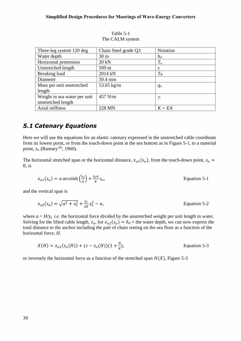
Table 5-1

The CALM system

Three-leg system 120 deg Chain Steel grade Q3 Notation

Water depth 30 m hd

Horizontal pretension 20 kN To

Unstretched length 509 m s

Breaking load 2014 kN TB

Diameter 50.4 mm

Mass per unit unstretched

length

53.65 kg/m qo

Weight in sea water per unit

unstretched length

457 N/m γr

Axial stiffness 228 MN K = EA

5.1 Catenary Equations

Here we will use the equations for an elastic catenary expressed in the unstretched cable coordinate

from its lowest point, or from the touch-down point at the sea bottom as in Figure 5-1, to a material

point, so. (Ramseyxlii, 1960).

The horizontal stretched span or the horizontal distance, 𝑥𝑜1(𝑠𝑜), from the touch-down point, 𝑠𝑜 =0, is

𝑥𝑜1(𝑠𝑜) = 𝑎 arcsinh (𝑠𝑜

𝑎) +

𝛾𝑟𝑎

𝐾𝑠𝑜, Equation 5-1

and the vertical span is

𝑥𝑜2(𝑠𝑜) = √𝑎2 + 𝑠𝑜2 +

𝛾𝑟

2𝐾𝑠𝑜

2 − 𝑎, Equation 5-2

where a = H/𝛾𝑟 i.e. the horizontal force divided by the unstretched weight per unit length in water.

Solving for the lifted cable length, 𝑠𝑜, for 𝑥𝑜2(𝑠𝑜) = ℎd = the water depth, we can now express the

total distance to the anchor including the part of chain resting on the sea floor as a function of the

horizontal force, H.

𝑋(𝐻) = 𝑥𝑜1(𝑠𝑜(𝐻)) + (𝑠 − 𝑠𝑜(𝐻))(1 +𝐻

𝐾), Equation 5-3

or inversely the horizontal force as a function of the stretched span 𝐻(𝑋), Figure 5-3


31

Figure 5-2

The horizontal force as a function of the horizontal stretched span.

In the intended system we have assumed a pretension of Hp = 20 kN at zero excursion. This

corresponds to a horizontal span of X(Hp) = 498.36 m. Finally we can add the reaction of the three

legs to get the total horizontal mooring force as a function of the excursion, x = X(H) - X(Hp), in the

x-direction in parallel to the upwind leg.

𝐹𝑡𝑜𝑡(𝐻) = 𝐻(𝑥) − 2cos (60°)𝐻(−𝑥

cos (60°) ), Equation 5-4

Figure 5-3

Horizontal force as a function of the excursion of the buoy.

The up-wave cable takes most of the load.

Figure 5-4

Horizontal force as a function of the excursion of the buoy.

Different range of vertical axis compared to Figure 5-3


32

In the example we can see that almost all the horizontal load is carried by the cable in the up-wave

direction as soon as the excursion exceeds 4 m.

Last we need calculate the horizontal stiffness, S(x), of the mooring system, that is, the slope of the

function displayed in Figure 5-4 and Figure 5-5.

Figure 5-6

The horizontal stiffness of the mooring system as a function of the excursion.

It is interesting to note that the stiffness for negative excursion is larger than for positive excursion,

which is caused by having two interacting legs in this direction.

5.2 Mean Excursion

The horizontal motion should be calculated around the mean offset (excursion). Therefore the offset

due to the mean forces is calculated using the methods described above. We also need the mooring

stiffness around the mean offset. The results are given in Table 5-2.

Table 5-2

Summary of offset and mooring stiffness due to the mean environmental forces

Mean force Force (kN) Mean offset (m) Tangential

Stiffness (kN/m)

Wind+current+Maximum

wave drift

10.5+24.5+108 =

= 143 6.45 68

Wind+current+WADAM

wave drift

10.5+24.5+2.5 =

= 37.5 2.63 12


33

6 Response Motion of the Moored Structure

6.1 Equation of Motion

The loads on a floating body can be constant as the mean load in Paragraph 5.2, transient i.e. of

short duration or harmonic. Irregular or random loads from e.g. sea waves can to a first, linear

approximation be treated as a superposition of harmonic loads, an approach that will be used here.

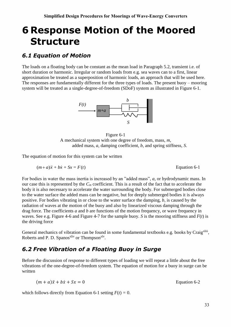
The responses are fundamentally different for the three types of loads. The present buoy – mooring

system will be treated as a single-degree-of-freedom (SDoF) system as illustrated in Figure 6-1.

m+a

F(t) b

S

Figure 6-1

A mechanical system with one degree of freedom, mass, m,

added mass, a, damping coefficient, b, and spring stiffness, S.

The equation of motion for this system can be written

)()( t + Sx = Fx + bxam Equation 6-1

For bodies in water the mass inertia is increased by an ”added mass”, a, or hydrodynamic mass. In

our case this is represented by the Cm coefficient. This is a result of the fact that to accelerate the

body it is also necessary to accelerate the water surrounding the body. For submerged bodies close

to the water surface the added mass can be negative, but for deeply submerged bodies it is always

positive. For bodies vibrating in or close to the water surface the damping, b, is caused by the

radiation of waves at the motion of the buoy and also by linearized viscous damping through the

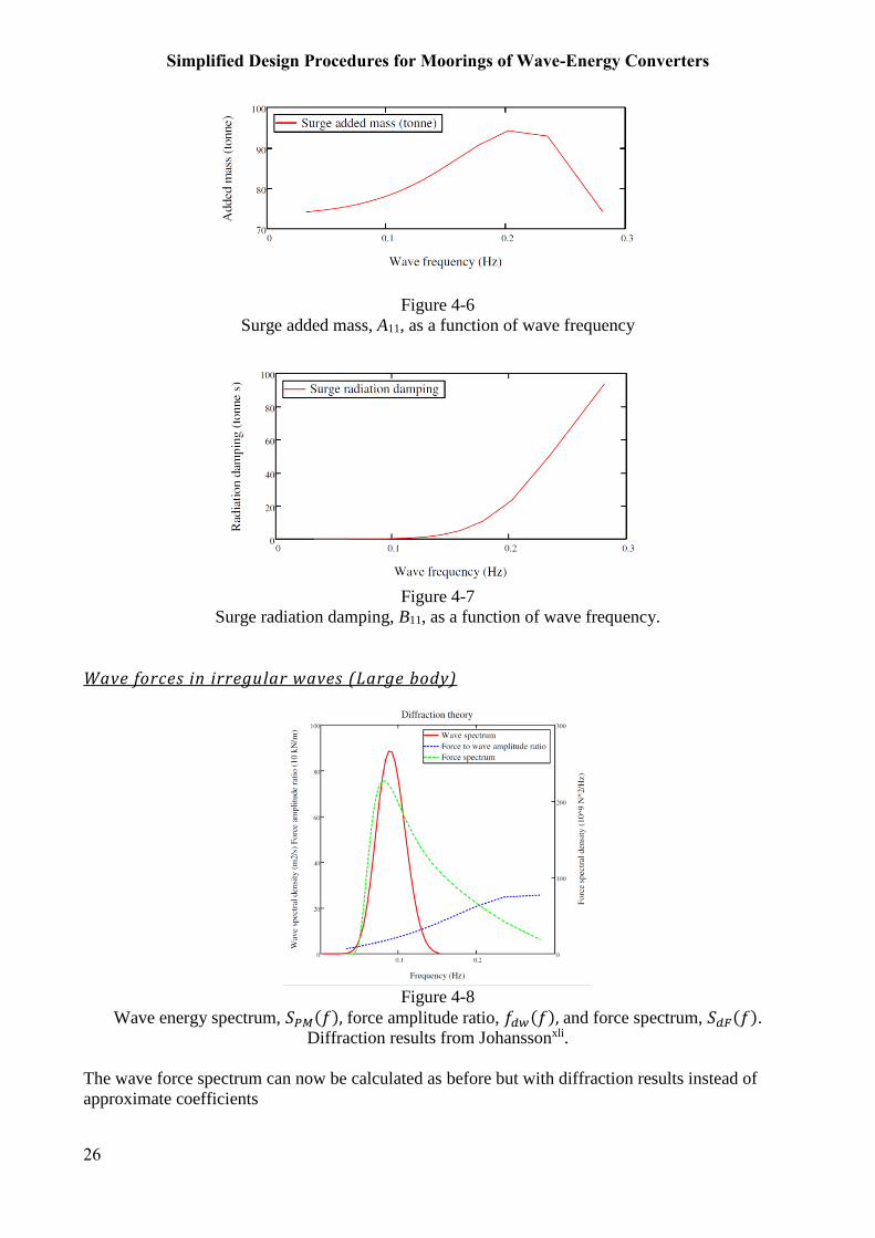
drag force. The coefficients a and b are functions of the motion frequency, or wave frequency in

waves. See e.g. Figure 4-6 and Figure 4-7 for the sample buoy. S is the mooring stiffness and F(t) is

the driving force

General mechanics of vibration can be found in some fundamental textbooks e.g. books by Craigxliii,

Roberts and P. D. Spanosxliv or Thompsonxlv.

6.2 Free Vibration of a Floating Buoy in Surge

Before the discussion of response to different types of loading we will repeat a little about the free

vibrations of the one-degree-of-freedom system. The equation of motion for a buoy in surge can be

written

(𝑚 + 𝑎)�̈� + 𝑏�̇� + 𝑆𝑥 = 0 Equation 6-2

which follows directly from Equation 6-1 setting F(t) = 0.


34

Assuming a solution of the form

tx = Ce , Equation 6-3

we get the characteristic equation

02 22 NN , Equation 6-4

where

)/( amSN is the “natural” angular frequency, that is, the undamped angular

frequency and

)(2/ amSb is the damping factor.

The roots of 02 22 NN , Equation

6-4 are

12

2,1 NN . Equation 6-5

These roots are complex, zero or real depending on the value of . The damping factor can thus be

used to distinguish between three cases: underdamped (0 < < 1), critically damped ( = 1) and

overdamped ( > 1). See Figure 6-2 for the motion of a body released from the position x(0) = 1 m

at t = 0 s. The underdamped case displays an attenuating oscillation, while the other cases display

motions monotonously approaching the equilibrium position. A moored floating buoy in surge

would normally display underdamped characteristics with a damping factor of the order of 10-3.

Note that an unmoored buoy, S = 0 exhibits no surge resonance. The damping factor is often called

the damping ratio, as it is equal to the ratio between the current damping coefficient, b, and the

critical damping coefficient, )(2 amc .

Figure 6-2

Response of a damped SDOF system with various damping ratios.

= 1.5

= 1

= 0.1


35

Table 6-1

Natural frequencies and damping factors for the moored buoy at the two mean offsets.

Mean offset (m) Stiffness (kN/m) Natural frequency (s) Damping factor

6.90 68.0 (Tangential) 10.2 1.3∙10-3

3.89 12.0 (Tangential) 19.9 0.17∙10-30

200 (Secant) 6 75∙10-3

The natural frequencies and damping factors for the moored buoy at the two mean offsets are listed

in Table 6-1. As the peak period is Tp = 12.9 s and the zero-crossing period is Tz = 10.1 s in the

design spectrum, there is a risk of large horizontal resonance motion. In the table there is also a

secant modulus listed, which is the mean stiffness for an excursion from 4.5 to 14 m, when the

whole chain is lifted.

6.3 Response to Harmonic Loads

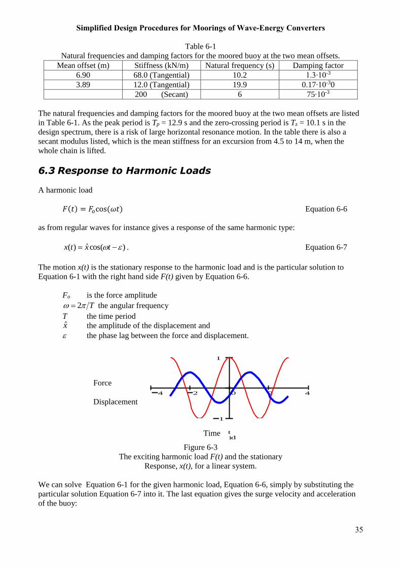
A harmonic load

𝐹(𝑡) = 𝐹𝑜cos (𝜔𝑡) Equation 6-6

as from regular waves for instance gives a response of the same harmonic type:

)cos(ˆ)( txtx . Equation 6-7

The motion x(t) is the stationary response to the harmonic load and is the particular solution to

Equation 6-1 with the right hand side F(t) given by Equation 6-6.

Fo is the force amplitude

T 2 the angular frequency

T the time period x the amplitude of the displacement and

the phase lag between the force and displacement.

Figure 6-3

The exciting harmonic load F(t) and the stationary

Response, x(t), for a linear system.

We can solve Equation 6-1 for the given harmonic load, Equation 6-6, simply by substituting the

particular solution Equation 6-7 into it. The last equation gives the surge velocity and acceleration

of the buoy:

4 2 0 2 4

1

1

Tid

Kraft

, för

skjut

ning

F( )t

x( )t

t

Force

Displacement

Time


36

x x t

x x t

x x t

cos( )

sin( )

cos( )

2

The substitution gives

)cos()sin(ˆ)cos(ˆ))(( 2 tFtxbtxamS o Equation 6-8

Using the trigonometric expressions for sine and cosine of angle differences then yields after some

manipulation the amplitude x , which by definition is positive.

2222)(

ˆ

bamS

Fx o

Equation 6-9

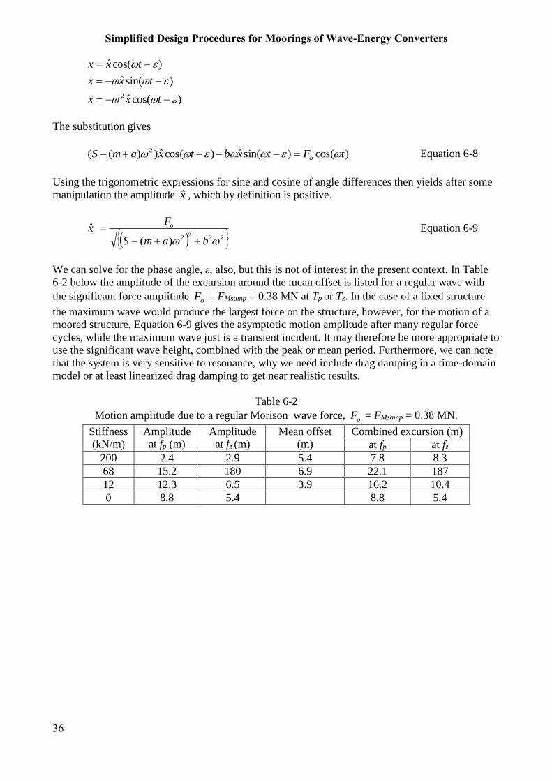
We can solve for the phase angle, ε, also, but this is not of interest in the present context. In Table

6-2 below the amplitude of the excursion around the mean offset is listed for a regular wave with

the significant force amplitude oF = FMsamp = 0.38 MN at Tp or Tz. In the case of a fixed structure

the maximum wave would produce the largest force on the structure, however, for the motion of a

moored structure, Equation 6-9 gives the asymptotic motion amplitude after many regular force

cycles, while the maximum wave just is a transient incident. It may therefore be more appropriate to

use the significant wave height, combined with the peak or mean period. Furthermore, we can note

that the system is very sensitive to resonance, why we need include drag damping in a time-domain

model or at least linearized drag damping to get near realistic results.

Table 6-2

Motion amplitude due to a regular Morison wave force, oF = FMsamp = 0.38 MN.

Stiffness

(kN/m)

Amplitude

at fp (m)

Amplitude

at fz (m)

Mean offset

(m)

Combined excursion (m)

at fp at fz

200 2.4 2.9 5.4 7.8 8.3

68 15.2 180 6.9 22.1 187

12 12.3 6.5 3.9 16.2 10.4

0 8.8 5.4 8.8 5.4


37

Figure 6-4

The horizontal response amplitude ratio, surge motion amplitude divided by the wave force

amplitude, as a function of frequency. The frequencies corresponding to the peak and mean periods

are marked to point out the sensitivity to the loading frequency.

6.4 Response Motion in Irregular Waves

6.4.1 Morison mass approach

Using the wave force spectrum based on the Morison mass force approach

𝑆𝐹(𝑓) = (𝑓𝑤(𝑓))2

𝑆𝑃𝑀(𝑓), Equation 6-10

we can calculate the surge motion response spectrum asxxxix

𝑆𝑥(𝑓) =𝑆𝐹(𝑓)

(𝑆−(𝑚+𝑎)𝜔2)2+𝑏2𝜔2=

(𝑓𝑤(𝑓))2

𝑆𝑃𝑀(𝑓)

(𝑆−(𝑚+𝑎)𝜔2)2+𝑏2𝜔2 Equation 6-11

Then the significant motion amplitude can be estimated as

𝑥1𝑠 = 2√𝑚0𝑑𝐹 = 2√∑ 𝑆𝑥(𝑓𝑖)∆𝑓𝑖𝑖 Equation 6-12

The result of this calculation is shown in Figure 6-5 and in Table 6-3 below on the lines marked

“none” under linearized drag damping. Without consideration of the drag damping the motion

becomes unrealistically large as the large horizontal drag damping is not taken into account. It is

much larger than the surge radiation damping.


38

Figure 6-5

Motion spectra, wave spectrum and force spectrum as functions of frequency.

Morison mass approach. No viscous damping.

Table 6-3

Significant linear response in an irregular wave, PM-spectrum, Hs = 8.3 m.

Mean offset

(m)

Stiffness

(kN/m)

Linearized drag

damping

Significant

amplitude (m)

5.4 Morison 200 none 7.4

6.9 68 none 37.7

3.9 12 none 7.3

5.4 Diffraction 200 none 3.0

6.9 68 none 31.5

3.9 12 none 9.5

5.4 200 included 2.3

6.9 68 included 5.3

3.9 12 included 5.2

6.4.2 Diffraction force approach

Using the wave force spectrum based on diffraction forces we can similarly form a diffraction-

based surge spectrum:

𝑆𝑑𝐹(𝑓) = (𝑓𝑑𝑤(𝑓))2

𝑆𝑃𝑀(𝑓), Equation 6-13

we can calculate the surge motion response spectrum asxxxix

𝑆𝑑𝑥(𝑓) =𝑆𝑑𝐹(𝑓)

(𝑆−(𝑚+𝑎)𝜔2)2+𝑏2𝜔2 =(𝑓𝑑𝑤(𝑓))

2𝑆𝑃𝑀(𝑓)

(𝑆−(𝑚+𝑎)𝜔2)2+𝑏2𝜔2 Equation 6-14

Then the significant motion amplitude can be estimated as


39

𝑥𝑑1𝑠 = 2√𝑚0𝑑𝐹 = 2√∑ 𝑆𝑥(𝑓𝑖)∆𝑓𝑖𝑖 Equation 6-15

The result of this calculation is shown in Figure 6-6 below and in Table 6-3 above on the lines

marked diffraction and “none” under linearized drag damping. Without consideration of the drag

damping the motion becomes also here unrealistically large.

Figure 6-6

Motion spectra and wave spectrum as functions of frequency.

Diffraction approach. No viscous damping.

6.5 Equivalent Linearized Drag Damping

Neglecting the coupling between surge and pitch we can symbolically write the drag damping surge

force as

111 xuxuKFD , Equation 6-16

where K can be set to (1/2)CDDhb and u is the undisturbed horizontal velocity of the water in the

surge direction and 1x the surge velocity of the buoy.

When the non-linear surge damping is important usually 1xu and then we can set

𝐹𝐷1 = 𝐾|�̇�1|(�̇�1), Equation 6-17

which is simpler but still non-linear.

To assess an equivalent linear coefficient we can compare the dissipated energy over a time, say

3 h, with an equivalent linear expression and the surge velocity

𝑥1(𝑡) = ∑ (√2𝑆𝑥(𝑓𝑖)∆𝑓𝑖𝑖 cos (𝜔𝑖𝑡 + 𝜀𝑖)) Equation 6-18


40

Then the dissipated energy can be calculated in two ways

T

e

T

dtxBdtxxK0

2

111

0

2

11 , Equation 6-19

T

T

e

dtx

dtxx

KB

0

2

1

0

2

11

11

Equation 6-20

That is, the equivalent damping coefficient, Be11, depends on the modulus of the surge motion 1x .

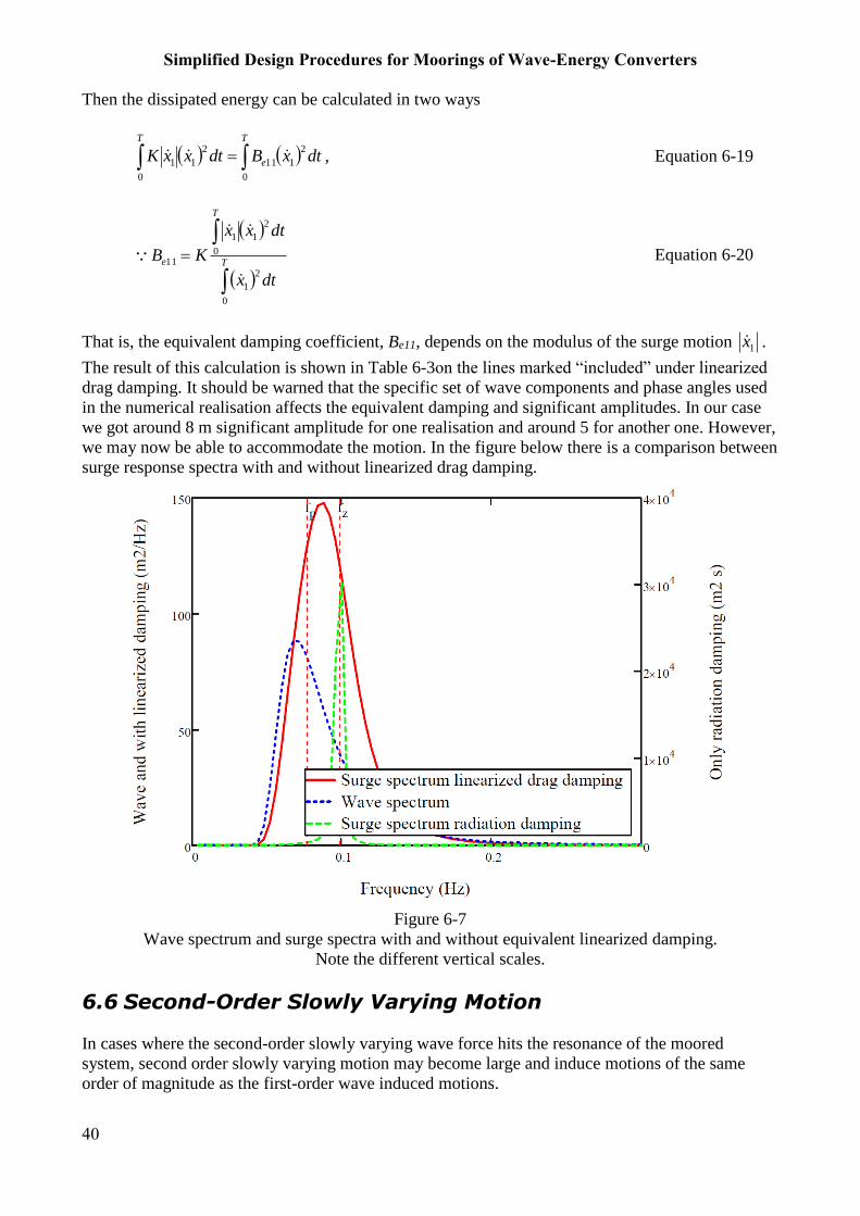
The result of this calculation is shown in Table 6-3on the lines marked “included” under linearized

drag damping. It should be warned that the specific set of wave components and phase angles used

in the numerical realisation affects the equivalent damping and significant amplitudes. In our case

we got around 8 m significant amplitude for one realisation and around 5 for another one. However,

we may now be able to accommodate the motion. In the figure below there is a comparison between

surge response spectra with and without linearized drag damping.

Figure 6-7

Wave spectrum and surge spectra with and without equivalent linearized damping.

Note the different vertical scales.

6.6 Second-Order Slowly Varying Motion

In cases where the second-order slowly varying wave force hits the resonance of the moored

system, second order slowly varying motion may become large and induce motions of the same

order of magnitude as the first-order wave induced motions.


41

The low-frequency excitation force can be expressed in the frequency-domain by a spectrum

(Pinkster, 1975)xlvi.

𝑆𝐿𝐹(𝜇) = 8 ∫ 𝑆(𝜔)∞

0𝑆(𝜔 + 𝜇)𝐶𝑑 (𝜔 +

𝜇

2) dω Equation 6-21

Here 𝑆(𝜔) is the wave spectrum and 𝐶𝑑(𝜔) is the wave-drift force coefficient. The equation is

invoking the Newmanxlvii approximation and cannot be used if the resonance period is within the

wave spectrum periods. Then the full non-linear expression should be used. See e.g. Faltinsen

(1990)xxxiii. In the present case this is not the case and, anyway, in such cases the motion is

dominated by the first-order wave-excited motion.

A sample calculation for this case gives negligible second order slowly varying motion

– surge amplitude less than a < mm – compared to the first-order motion. They can be comparable

in lower sea states. The reason for negligible second order slowly varying motion is that the

resonance period is off the peak of the drift-force spectrum and that the drift force coefficient is

small. On the other hand, we should maybe have used the full non-linear expression. However,

experience gives that the second-order motions for small objects in high sea states display little

second-order motions. See the figure below, where the horizontal resonances at 0.3 and 0.6 rad/s for

the two offset tensions pretensions are marked.

Figure 6-8

Drift-force spectrum, drift-force coefficient and wave spectrum as functions of angular frequency.

6.7 Wave-Drift Damping

In forward speed and in coastal currents the slowly varying motion may be damped by the fact that

the encountered wave period and subsequently the wave drift coefficient varies during the slow

surge causing a kind of hysteretic damping, called wave-drift damping. As we have negligibly small

slowly varying motion in the present case, it is not useful to take this into account.

6.8 Combined Maximum Excursions

Using the design format according to Equation 2-1 we end up with the following table over the

design motions XC1 and XC2.


42

XC1 = Xmean + XLF-max + XWF-sig

XC2 = Xmean + XLF-sig + XWF-max Equation 2-1

Table 6-4

Design offsets for quasi-static design. Diffraction results with equivalent drag damping

Stiffness

(kN/m)

Mean

offset (m)

Wave-frequency

amplitude (m)

Low-frequency

amplitude (m)

Design offset

(m)

Lifted chain

length (m) at

XC2

Sign. Max. Sign. Max. XC1 XC2

200 4 2.3 4.3 6.3 8.3 219

68 6.5 5.3 9.9 0 0 11.8 16.4 624 (> 509)

12 2.6 5.2 9.7 0 0 7.8 12.3 424

The calculation shows that if we use the secant stiffness modulus and the small modulus (12 kN/m)

of the mooring system we fulfil the lifting criterion that the up-wave chain should rest on the

bottom close to the anchor: For the stiffer case (68 kN/m) case the chain of the chosen mooring

system will lift all the way to the anchor. We would have to modify the mooring system by

choosing longer and maybe heavier chains, increasing the number of mooring legs or choosing

softer synthetic mooring lines to accommodate the offsets. However, it remains to check the tension

requirement

.


43

7 Required Minimum Breaking Strength

As described in Paragraph 2.2 the calculated tension TQS(XC) should be multiplied by a partial safety

factor γ = 1.7 for Consequence Class 1 and the product should be less than 0.95 times the minimum

breaking strength, Smbs, when statistics of the breaking strength of the component are not available:

γTQS < 0.95Smbs Equation 2-2

Another usual expression is the utilisation factor

u =γTQS

0.95Smbs< 1 Equation 2-3

The results of the design calculation is given in Table 7-1. As can be seen only the calculation with

the secant modulus S = 200 kN/m meets the requirements. However, this calculation is not

according to the standard procedure and may not be accepted. The secant modulus should at least be

changed to a value based on the resulting maximum excursion. Solving Equation 2-2 for the

minimum breaking strength with TQS = 1.38 MN gives a required minimum breaking strength to 2.5

MN. This corresponds to a chain G3 58 mmxlviii with 𝑆𝑚𝑏𝑠 = 2.6 MN and a mass of 77 kg/mxlix. A

second design loop should be performed with this chain and diffraction methods including

linearised damping. If necessary more loops should be performed.

Table 7-1

Comparison between required tension and calculated tension

Stiffness

(kN/m)

Design offset

(m)

Lifted chain

length (m) at XC2 𝑇𝑄𝑆

(MN)

𝛾𝑇𝑄𝑆

(MN)

0.95𝑆𝑚𝑏𝑠 (MN)

u

XC1 XC2

200 6.3 8.3 219 0.37 0.63 1.9 0.33

68 11.8 16.4 624 3.01 5.12 1.9 2.69

12 7.8 12.3 424 1.38 2.35 1.9 1.23


44

8 Conclusions

The following conclusions can be drawn from the design exercise

Simplified drag and wind coefficients can be used, because the mean offset is not a dominant

part of the total horizontal displacement.

The Morison wave formulation can be used for objects smaller than a 5th of the wavelength,

however with some overdesign. It is important to test various wave frequencies and realistic

wave amplitudes. Used in the frequency-domain, skipping the drag component, equivalent

linearized drag damping must be added.

Also using the diffraction method for small objects, equivalent linearized drag damping must be

added.

In the equation of motion, there is a difficulty with progressive stiffening moorings. In the

CALM system choosing a stiffness around the mean offset will not give a realistic motion as the

stiffness may vary one order of magnitude during the oscillation. It is advised to use time-

domain simulations taking at least S(x) into consideration, and then the drag damping could as

well be introduced as 𝑏(�̇�) = 𝐶𝐴½𝜌|�̇�|. In a final design time-domain design tools including mooring dynamics should be used

complemented by large scale model tests


45

9 Acknowledgements

The study is carried out at Dept. of Shipping and Marine Technology, Chalmers, and is co-funded

from Region Västra Götaland, Sweden, through the Ocean Energy Centre hosted by Chalmers

University of Technology, and the Danish Council for Strategic Research under the Programme

Commission on Sustainable Energy and Environment (Contract 09-067257, Structural Design of

Wave Energy Devices).


46

10 References i L. Bergdahl and P. McCullen “Development of a Safety Standard forWave Power Conversion

Systems” Wave Energy Network, CONTRACT N° : ERK5 - CT - 1999-2001, 2002 ii L. Bergdahl and N. Mårtensson ”Certification of wave-energy plants – discussion of existing

guidelines, especially for mooring design”, in Proceedings of the 2nd European Wave Power

Conference, pp. 114-118 Lisbon, Portugal, 1995 iii L. Johanning, G.H. Smith and J. Wolfram, ”Towards design standards for WEC moorings”, in

Proceedings of the 6th Wave and Tidal Energy Conference, Glasgow, Scotland, 2005 iv Paredes, G., Bergdahl, L., Palm, J., Eskilsson, C. & Pinto, F.: Station keeping design for floating

wave energy devices compared to floating offshore oil and gas platforms. Proceedings of the 10th

European Wave and Tidal Energy Conference 2013 v Position Mooring, DNV Offshore Standard DNV-OS-E301, 2013 vi Guidelines on design and operation of wave energy converters, Det Norske Veritas, 2005 (Carbon

Trust Guidelines) vii L.M. Bergdahl and I. Rask, “Dynamic vs. Quasi-Static Design of Catenary Mooring System”,

1987 Offshore Technology Conference, OTC 5530 viii M.J. Muliawan, Z. Gao and T. Moan, “Analysis of a two-body floating wave energy converter

with particular focus on the effect of power take off and mooring systems on energy capture”, in

OMAE 2011, OMAE2011-49135 ix Sesam, MIMOSA, DNV Softwares. [Online]. Available:

http://www.dnv.com/services/software/products/sesam/sesamdeepc/mimosa.asp, Visited 2013-03-

11 x Orcaflex Documentation. [Online]. Available:

http://www.orcina.com/SoftwareProducts/OrcaFlex/Documentation/OrcaFlex.pdf, Visited 2013-03-

11 xi ZENMOOR Mooring Analysis Software for Floating Vessels [Online]. Available:

http://www.zentech-usa.com/zentech/pdf/zenmoor.pdf

Visited 2013-03-12 xii Sesam SIMO, DNV Softwares. [Online]. Available:

http://www.dnv.com/services/software/products/sesam/sesamdeepc/simo.asp, Visited 2013-03-11 xiii Sesam, DeepC, DNV Softwares. [Online]. Available:

http://www.dnv.com/services/software/products/sesam/sesamdeepc/, Visited 2013-03-11 xiv S. Parmeggiano et al. "Comparison of mooring loads in survivability mode of the wave dragon

wave energy converter obtained by a numerical model and experimental data", in OMAE 2012,

OMAE2012-83415 xv CASH, In-house program, GVA. [Online]. Available: http://www.gvac.se/engineering-tools/,

Visited 2013-03-11 xvi Thunder Horse Production and Drilling Unit [Online] Available: http://www.gvac.se/thunder-

horse/, Visited 2013-03-11 xvii Z. Gao and T. Moan, “Mooring system analysis of multiple wave energy converters in a farm

configuration”, Proceedings of the 8th European Wave and Tidal Energy Conference, Uppsala,

Sweden, 2009 xviii D.J. Pizer et al. Pelamis WEC – Recent advances in the numerical and experimental modelling

programme, Proceedings of the 6th European Wave and Tidal Energy Conference, Glasgow, UK,

2005 xix Q.W. Ma and S. Yan, “QALE-FEM for numerical modelling of nonlinear interaction between

3D moored floating bodies and steep waves,”Int. J. Numer. Meth. Engng., vol. 78, pp. 713-756,

2009

http://www.orcina.com/SoftwareProducts/OrcaFlex/Documentation/OrcaFlex.pdf

http://www.zentech-usa.com/zentech/pdf/zenmoor.pdf

http://www.dnv.com/services/software/products/sesam/sesamdeepc/simo.asp

http://www.dnv.com/services/software/products/sesam/sesamdeepc/

http://www.gvac.se/thunder-horse/

http://www.gvac.se/thunder-horse/


47

xx J. Palm et al CFD Simulation of a Moored FloatingWave Energy Converter, Proceedings of the

10th European Wave and Tidal Energy Conference, Aalborg, Denmark, 2013 xxi Y. Yu & Y. Li, “Preliminary result of a RANS Simulation for a Floating Point Absorber Wave

Energy System under Extreme Wave Conditions”, in 30th International Conference on Ocean,

Offshore, and Arctic Engineering, Rotterdam, The Netherlands, June 19-24, 2011 xxii Jack/St Malo Deepwater Oil Project [Online]. Available: http://www.offshore-

technology.com/projects/jackstmalodeepwaterp/, Visited 2013-03-11 xxiii Jack & St Malo Project, “Response-based analysis”, GVA, KBR, Göteborg, 2010, Internal

report xxiv Recommended Practice DNV-RP-C205, October 2013 xxv Raphael Waters et al.: Wave climate off the Swedish west coast, Renewable Energy 34 (2009)

1600-1606 xxvi http://citeseerx.ist.psu.edu/viewdoc/download?doi=10.1.1.135.7884&rep=rep1&type=pdf ,

visited 2014-05-05. xxvii Peter Söderberg: The Swedish coastal wave climate, SSPA Report 104, 1987 xxviii Svensk Lots Del A Allmänna upplysningar, Sjöfartsverkets Sjökarteavdelning, Norrköping

1992 xxix Margheritini, L 2012, Review on Available Information on Waves in the DanWEC Area:

(DanWEC Vaekstforum 2011). Department of Civil Engineering, Aalborg University, Aalborg.

DCE Technical Reports, nr. 135 xxx Margheritini, L 2012, Review on Available Information on Wind, Water Level, Current, Geology

and Bathymetry in the DanWEC Area: (DanWEC Vaekstforum 2011). Department of Civil

Engineering, Aalborg University, Aalborg. DCE Technical Reports, nr. 136 xxxi Martin Sterndorf: WavePlane, Conceptual Mooring System Design, Sterndorf Engineering, 15

November 2009 xxxii A. Pecher, A. Foglia and J.P. Kofoed: Comparison and sensitivity investigations of a CALM

and SALM type mooring system for WECs. xxxiii O.M. Faltinsen: Sea Loads on Ships and Offshore Structures, Cambridge University Press,

1990. xxxiv Peter Sachs: Wind Forces in Engineering, Second Edition, 1978 Elsevier

ISBN: 978-0-08-021299-9 xxxv M.R. Haddara, C. Guedes Soares: Wind loads on marine structures, Marine Structures 12

(1999) 199-209 xxxvi Longuet-Higgins: The mean forces exerted by waves on floating or submerged bodies with

application to sand bars and wave-power machines. Proc. R. Soc. London, A352, 462-480 (1977) xxxvii H. Maruo: The drift of a body floating on waves, J. of Ship Research, Vol 4, 1960 xxxviii Sarpkaya, T. and Isaacson, M.: Mechanics of Wave Forces on Offshore Structures, Van

Nostrand Reinhold Company, 1981

ISBN 10: 0442254024 / ISBN 13: 9780442254025 xxxix Chakrabarti, S.K.: Handbook of offshore engineering, Vol. 1, Elsevier, 2005 xl R. Yeung, “Added mass and damping of a vertical cylinder in finite-depth waters”, Applied

Ocean Research, ISSN 0141-1187, 1981, Vol.3, No 3, pp. 119 - 133 xli Johansson, M.: Transient motion of large floating structures, Report Series A:14, Department of

Hydraulics, Chalmers University of Technology, 1986 xlii A.S. Ramsey: Statics, Cambridge, The University Press, 1960 xliii Roy R. Craig, Jr.: Structural Dynamics, John Wiley & Sons, New York, 1981 xliv J. B. Roberts and P. D. Spanos: Random vibration and statistical linearization, John Wiley &

Sons, Chichester, 1990 xlv William T. Thompson: Theory of Vibration with Applications, Prentice-Hall Inc., Englewood

Cliffs, 1972

http://www.offshore-technology.com/projects/jackstmalodeepwaterp/

http://www.offshore-technology.com/projects/jackstmalodeepwaterp/

http://citeseerx.ist.psu.edu/viewdoc/download?doi=10.1.1.135.7884&rep=rep1&type=pdf


48

xlvi J.A. Pinkster: Low-frequency Phenomena Associated with Vessels Moored at Sea. Society of

Petroleum Engineers Journal, Dec 487-494 xlvii J.N. Newman: Second Order Slowly Varying Forces on Vessels in Irregular Waves. Proc. of

International Symposium Dynamics of Marine Vehicles and Structures in Waves, Ed. R:E:D:

Bishop and W:G: Price pp. 182-186. London Mechanical Engineering Publications LTD, 1974 xlviii http://www.sotra.net/products/tables/stength-for-studlink-anchor-chain-cables, visited 2014-05-

22 xlix http://www.sotra.net/products/tables/weight-for-studlink-anchor-chain, visited 2014-05-22

http://www.sotra.net/products/tables/stength-for-studlink-anchor-chain-cables

http://www.sotra.net/products/tables/weight-for-studlink-anchor-chain

Date post:	13-Mar-2018
Category:	Documents
Upload:	vudieu
View:	215 times
Download:	1 times