Page 1
AALBORG UNIVERSITY
Master Thesis
MOBILE COMMUNICATIONS 2011
Can you fix the iPhone?
A study about the human body influence on the
performance of antennas and ways to parameterize this
influence
Under the supervision of: Dr. Mauro PELOSI
& Prof. Gert. F. Pedersen
Research conducted by and report written by:
Marc CORNUEJOLS, Guillaume VIGNAL and Arnaud ZEENDER
Page 2
Page 2
Abstract
In response to a lack of research in the domain of studies concerning the
impact of the human body on the performance of an antenna, this thesis
explores this impact. It also tries to determine a criterion concerning the
robustness of the antenna with regard of this impact. However it is
ultimately shown that their no real criterion, or rather an infinity of them
and that the robustness can only be found experimentally.
Signatures
Marc Cornuéjols
Guillaume Vignal
Arnaud Zeender
Page 3
Page 3
Table of Contents
LIST OF FIGURES .............................................................................................................................. 5
LIST OF TABLES .............................................................................................................................. 11
LIST OF SYMBOLS AND ABREVIATIONS ................................................................................ 12
INTRODUCTION ............................................................................................................................... 14
CHAPTER ONE: TOOLS OF MEASUREMENT AND SIMULATION ..................................... 16
I – Introduction ........................................................................................................................... 16
II – Power Dissipated ................................................................................................................ 17
1) Calculation methods of power dissipation ......................................................... 17
2) Total power dissipation ............................................................................................. 19
3) Power dissipation along an axis ............................................................................ 19
III – Three Dimensional Correlations .................................................................................. 20
1) Cross-correlation definition and explanation ................................................... 20
2) Interpretation of results ........................................................................................... 23
IV – S11 Parameter ................................................................................................................... 24
V – Imaginary Part ..................................................................................................................... 25
VI – Smith Chart ......................................................................................................................... 26
VI – Finding the appropriate brick ....................................................................................... 31
CHAPTER TWO: SIDE EXPERIMENTS ...................................................................................... 33
I – Conductivity, permittivity and permeability variations ......................................... 33
II – Narrowband PIFA study ................................................................................................... 38
III – Impact of the permittivity of the substrate on a thin substrate-layered
PIFA antenna ................................................................................................................................ 40
IV – Defining the composition of the human hand ........................................................ 43
CHAPTER THREE: SIMULATION PARADIGM AND ALTERATION .................................... 47
I – Introduction ........................................................................................................................... 47
II – Slicer ....................................................................................................................................... 47
III – Difference in power calculation ................................................................................... 48
IV – Changes brought to AAU3 ............................................................................................. 49
CHAPTER FOUR: COMPARISON OF REFERENCE ANTENNAS ......................................... 50
I – Introduction ........................................................................................................................... 50
II – Dipole ...................................................................................................................................... 51
Page 4
Page 4
III – Monopole ............................................................................................................................. 56
IV – PIFA ........................................................................................................................................ 61
V – Slotted PIFA .......................................................................................................................... 66
VI – Narrowband PIFA .............................................................................................................. 71
VII – PIFA with substrate ........................................................................................................ 76
VIII – IFA ....................................................................................................................................... 81
IX – Loop ........................................................................................................................................ 86
X – Folded loop ............................................................................................................................ 91
CHAPTER FIVE: PARAMETERISATION AND ROBUSTNESS CRITERION ..................... 96
I – Percentage of power dissipated ..................................................................................... 96
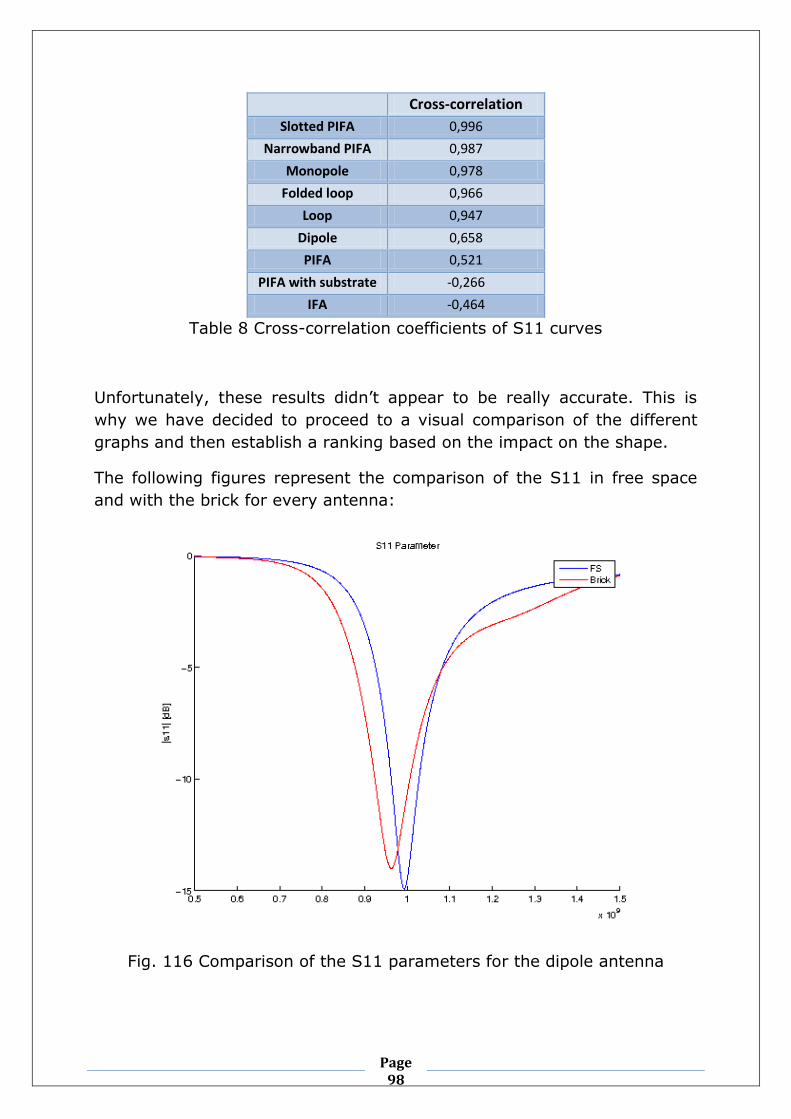
II – 3D Correlation of E-fields ................................................................................................ 97
III – General shape evaluation .............................................................................................. 97
IV – Variation of the resonant frequency and the associated S11 parameter . 103
V – Evolution of the Efficiency ............................................................................................. 104
VI – Global view of the rankings ........................................................................................ 105
CONCLUSION.................................................................................................................................. 106
References ....................................................................................................................................... 107
Page 5
Page 5
LIST OF FIGURES Fig. 1 User sensitive part of the iPhone 4 antenna P14
Fig. 2 Example sets A and B P21
Fig. 3 First cross-correlation coefficient computation on
overlapping cells P22
Fig. 4 Second cross-correlation coefficient computation P22
Fig. 5 Fourth cross-correlation coefficient computation P22
Fig. 6 A two port network representing a transmission line P24
Fig. 7 A S11 plot as a function of frequency P25
Fig. 8 Imaginary part of a dipole resonating at 1GHz P26
Fig. 9 Smith Chart P27
Fig. 10 Impedance circles P28
Fig. 11 Imaginary parts P28
Fig. 12 Impedance axes P29
Fig. 13 Total impedance P30
Fig. 14 Reflection coefficient at the transmission line P30
Fig. 15 Wavelength scale P31
Fig. 16 An AAU3 human hand design P32
Fig. 17 The simplified human hand model P32
Fig. 18 Scheme of the variations experiment, a PIFA antenna facing a
brick P34
Fig. 19 Relative power dissipation according to the variation of sigma P35
Page 6
Page 6
Fig. 20 Relative power dissipation according to the variations of
epsilon P36
Fig. 21 Relative power dissipation according to the variation of mu P36
Fig. 22 Power dissipation along the x-axis with a permeability of 42.5 P37
Fig. 23 Power dissipation along the x-axis with a permeability of 1.5 P37
Fig. 24 PIFA antennas separated by 1, 2, 5 and 10mm from the
ground plane P38
Fig. 25 Reflection coefficient for PIFA antennas elevated by 1, 2, 5 and
10mm P39
Fig. 26 Thin-layered substrate PIFA antenna P40
Fig. 27 Performance variation for substrate PIFA antennas with different
permittivity for the substrate P42
Fig. 28 Comparative experiments P43
Fig. 29 1st layer representing a fat layer, 2nd layer representing a
Tissue-Equivalent Liquid (TEL) P44
Fig. 30 1st layer representing a muscle, 2nd layer representing a bone P45
Fig. 31 1st layer and 2nd layer representing a TEL P45
Fig. 32 Paper results P46
Fig. 33 Regular field graph P48
Fig. 34 Slicer P48
Fig. 35 A free space dipole antenna design P51
Fig. 36 A brick close by the dipole P51
Fig. 37 Free space S11 for a dipole antenna P52
Fig. 38 Brick S11 for a dipole antenna P52
Fig. 39 Imaginary part of a free space dipole P53
Fig. 40 Brick imaginary part of a dipole P53
Fig. 41 Smith Chart of a free space dipole P54
Page 7
Page 7
Fig. 42 Brick Smith Chart of a dipole P54
Fig. 43 Power dissipated along axis X for a dipole P55
Fig. 44 The free space design of a monopole P56
Fig. 45 The brick design of a monopole P56
Fig. 46 S11 of a monopole in free space P57
Fig. 47 Brick S11 of a monopole P58
Fig. 48 Imaginary part of a free space monopole P58
Fig. 49 Brick imaginary part of a monopole P58
Fig. 50 Smith Chart for a free space monopole P59
Fig. 51 Brick Smith Chart for a monopole P59
Fig. 52 Power dissipated along x for a monopole P60
Fig. 53 The free space design of a PIFA P61
Fig. 54 The brick design of a PIFA P61
Fig. 55 S11 of a PIFA in free space P62
Fig. 56 Brick S11 of a PIFA P62
Fig. 57 Imaginary part of a free space PIFA P63
Fig. 58 Brick imaginary part of a PIFA P63
Fig. 59 Smith Chart for a free space PIFA P64
Fig. 60 Brick Smith Chart for a PIFA P64
Fig. 61 Power dissipation along x for a PIFA P65
Fig. 62 The free space design of a slotted PIFA P66
Fig. 63 The brick design of a slotted PIFA P66
Fig. 64 S11 of a slotted PIFA in free space P67
Fig. 65 Brick S11 of a slotted PIFA P67
Fig. 66 Imaginary part of a free space slotted PIFA P68
Fig. 67 Brick imaginary part of a slotted PIFA P68
Page 8
Page 8
Fig. 68 Smith Chart for a free space slotted PIFA P69
Fig. 69 Brick Smith Chart for a slotted PIFA P69
Fig. 70 Power dissipation along x for a slotted PIFA P70
Fig. 71 The free space design of a narrowband PIFA antenna P71
Fig. 72 The brick design of a narrowband PIFA antenna P71
Fig. 73 S11 of a narrowband PIFA antenna in free space P72
Fig. 74 Brick S11 of a narrowband PIFA antenna P72
Fig. 75 Imaginary part of a free space narrowband PIFA antenna P73
Fig. 76 Brick imaginary part of a narrowband PIFA antenna P73
Fig. 77 Smith Chart for a free space narrowband PIFA antenna P74
Fig. 78 Brick Smith Chart for a narrowband PIFA antenna P74
Fig. 79 Power dissipation along x for a narrowband PIFA P75
Fig. 80 The free space design of a PIFA with substrate P76
Fig. 81 The brick design of a PIFA with substrate P76
Fig. 82 S11 of a PIFA with substrate in free space P77
Fig. 83 Brick S11 of a PIFA with substrate P77
Fig. 84 Imaginary part of a free space PIFA with substrate P78
Fig. 85 Brick imaginary part of a PIFA with substrate P78
Fig. 86 Smith Chart for a free space PIFA with substrate P79
Fig. 87 Brick Smith Chart for a PIFA with substrate P79
Fig. 88 Power dissipation along x for a PIFA with substrate P80
Fig. 89 The free space design of an IFA P81
Fig. 90 The brick design of an IFA P81
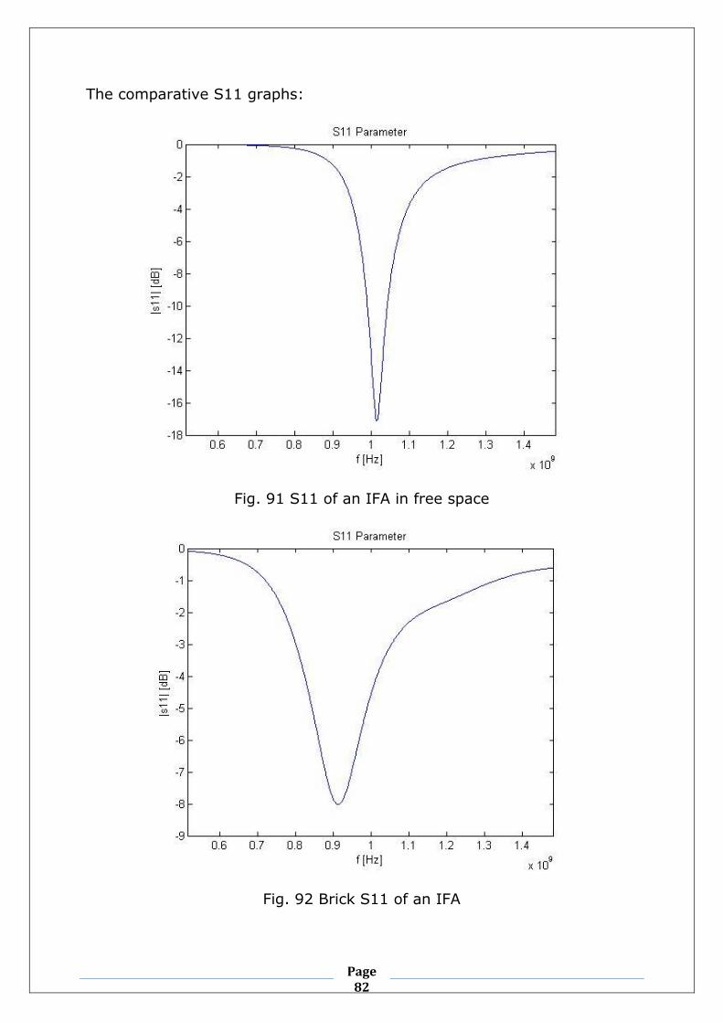
Fig. 91 S11 of an IFA in free space P82
Fig. 92 Brick S11 of an IFA P82
Fig. 93 Imaginary part of a free space IFA P83
Page 9
Page 9
Fig. 94 Brick imaginary part of an IFA P83
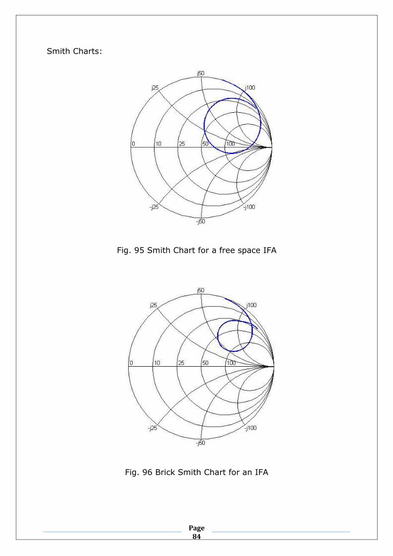
Fig. 95 Smith Chart for a free space IFA P84
Fig. 96 Brick Smith Chart for an IFA P84
Fig. 97 Power dissipation along x for an IFA P85
Fig. 98 The free space design of a loop P86
Fig. 99 The brick design of a loop P86
Fig. 100 S11 of a loop in free space P87
Fig. 101 Brick S11 of a loop P87
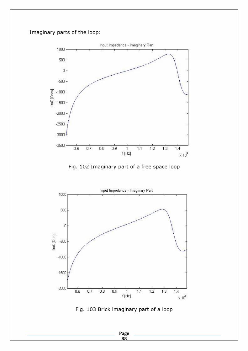
Fig. 102 Imaginary part of a free space loop P88
Fig. 103 Brick imaginary part of a loop P88
Fig. 104 Smith Chart for a free space loop P89
Fig. 105 Brick Smith Chart for a loop P89
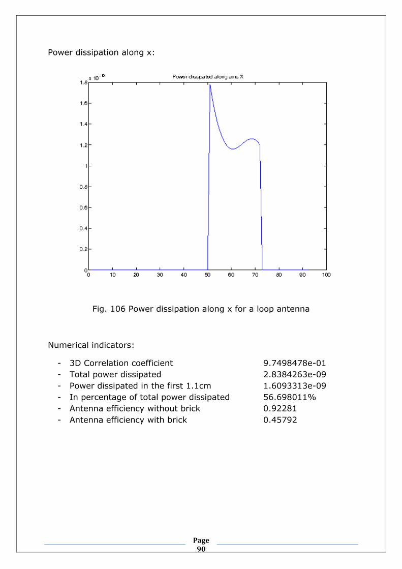
Fig. 106 Power dissipation along x for a loop antenna P90
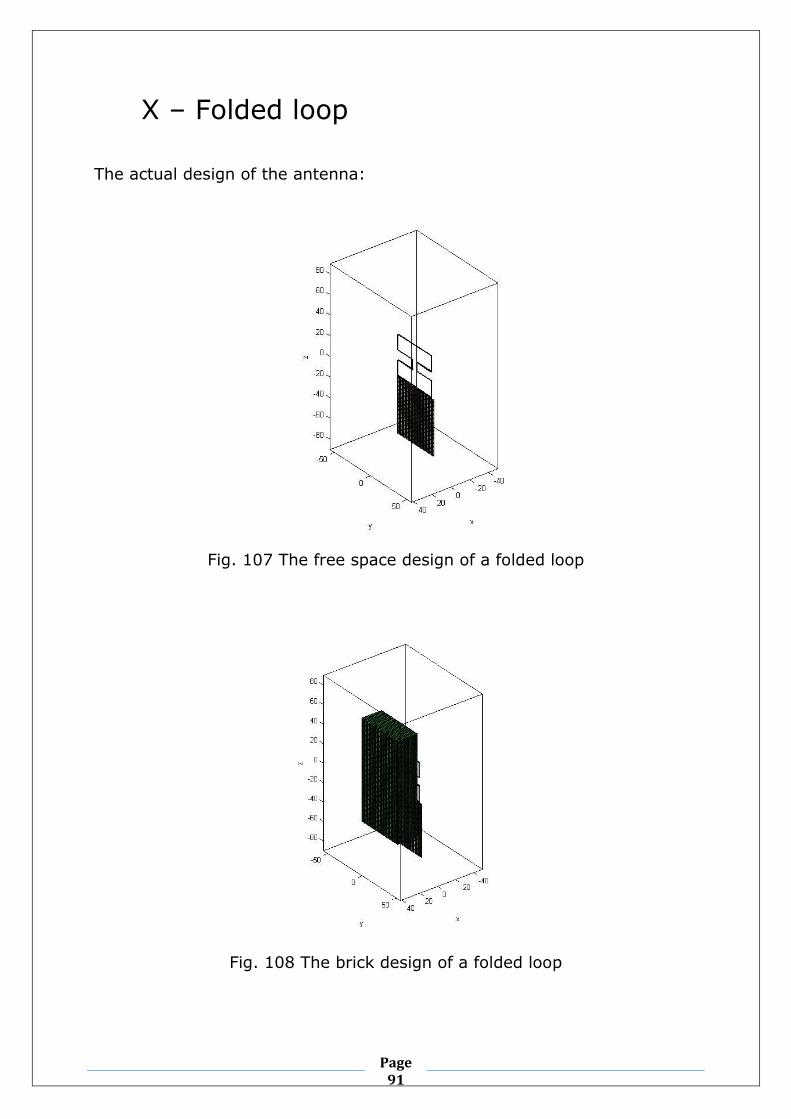
Fig. 107 The free space design of a folded loop P91
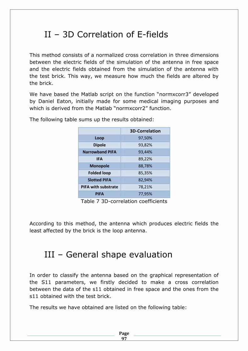
Fig. 108 The brick design of a folded loop P91
Fig. 109 S11 of a folded loop in free space P92
Fig. 110 Brick S11 of a folded loop P92
Fig. 111 Imaginary part of a free space folded loop P93
Fig. 112 Brick imaginary part of a folded loop P93
Fig. 113 Smith Chart for a free space folded loop P94
Fig. 114 Brick Smith Chart for a folded loop P94
Fig. 115 Power dissipation along x for a folded loop antenna P95
Fig. 116 Comparison of the S11 parameters for the dipole antenna P98
Fig. 117 Comparison of the S11 parameters for the folded loop
antenna P99
Fig. 118 Comparison of the S11 parameters for the IFA antenna P99
Page 10
Page 10
Fig. 119 Comparison of the S11 parameters for the loop antenna P100
Fig. 120 Comparison of the S11 parameters for the monopole
Antenna P100
Fig. 121 Comparison of the S11 parameters for the PIFA antenna P101
Fig. 122 Comparison of the S11 parameters for the narrowband PIFA
antenna P101
Fig. 123 Comparison of the S11 parameters for the slotted PIFA
antenna P102
Fig. 124 Comparison of the S11 parameters for the PIFA with substrate
antenna P102
Page 11
Page 11
LIST OF TABLES
Table 1 Results of the variations experiment _________ _____P35
Table 2 Impact of distance from the ground plane on PIFA antenna
performance _________________________________P39
Table 3 Performance variation of a thin-layered substrate PIFA antenna
with a change of permittivity of the substrate _________ P41
Table 4 Values of specific hand components _________ P42
Table 5 Error calculation between computation techniques _ P49
Table 6 Power dissipated for the different antennas P96
Table 7 3D-correlation coefficients P97
Table 8 Cross-correlation coefficients of S11 curves P98
Table 9 Visual ranking P103
Table 10 Resonant frequencies for the different antennas P103
Table 11 S11 variations P104
Table 12 Antennas efficiencies P104
Table 13 Antennas final rankings P105
Page 12
Page 12
LIST OF SYMBOLS AND ABREVIATIONS
Wi: The instantaneous Pointing vector
Ei: The instantaneous Electric field
Hi: The instantaneous Magnetic field
Pi: The instantaneous total power
s: A closed surface crossed by the electric and magnetic fields
Wav: The average Pointing vector
Wrad: The radiated Pointing vector
Pav: The average power
Prad: The radiated power
p: The dissipated power
σ: The conductivity
dk: The defined space step for the FDTD analysis along the axis k
rxy: The correlation coefficient
i: The value of the variable at a given point
i: The value of the variable at a given point
: The mean of
: The mean of
: The sample standard deviation of variables
: The sample standard deviation of variables
: The reflection coefficient.
Z0: The characteristic impedance of the transmission line
Page 13
Page 13
ZA: The impedance at the input of the antenna
Z: The impedance of the antenna
R: The real part of the impedance of the antenna
X: The imaginary part of the impedance of the antenna
FDTD: Finite Difference Time Domain
Epsilon: Permittivity
Sigma: Conductivity
Mu: Permeability
PIFA: Planar Inverted F Antenna
IFA: Inverted F Antenna
Page 14
Page 14
INTRODUCTION
Ever since the dawn of wireless communications, antennas have been
crucial in the process of designing efficient wireless systems. Being both
the transmitting and receiving appendixes of the overall network, their
performance has over the years been thoroughly investigated and
numerous antenna designs have been thought and/or implemented.
When considering the case of mobile handset antennas, engineers must
face additional challenges, size being the most important of them.
Therefore, constructors have at their disposal quantity of simulators and a
vast number of theoretical or experimental parameters to foresee the
overall quality of a design.
Fig. 1 User sensitive part of the iPhone 4 antenna
Yet with all these means at their disposal, one of the most important
failures still today is the case of the iPhone 4. Why did this unforeseen
error happen, and could it have been avoided?
The particularity of the iPhone 4 antenna is that rather than being internal
as in many mobile phones, it is actually situated on the outer boundary of
the mobile phone. And yet, this design said to be one of the most efficient
Apple had ever realized came out to be a near disaster.
Page 15
Page 15
The fact is that, as for almost any mobile phone antenna, its design had
been thought in free space, and it was most likely tested in experimental
free space. This is the reason of the failure of this antenna; it was not
considering the impact of the hand when a user was holding the phone.
While this error of implementation could have been avoided via
experimentation with actual user body interference, it mainly shows a lack
of consideration from mobile phone companies for the said impact.
However, this situation has forced manufacturers to deepen their
knowledge about user interference and to focus more consequently on this
issue.
In this context, this thesis acts as a study on the impact of the body of the
user on antennas and tries to determine a simulation level parameter that
could indicate whether or not an antenna is robust to this impact. The
main idea around this study being to avoid antenna manufacturers from
having to experiment blindly on the topic, benefiting from a trend idea
given by the parameter.
Firstly, a rough description is given about the FDTD implementation
software used to conduct this research. Then, the tools of measurement
investigated and used are described, followed by other leads research has
required but which had only intermediate or little impact on the choice of
a robustness parameter.
Secondly, reference antennas are described and analyzed through all
“lenses” described in the previous section. They are then all compared and
ranked by robustness with regard of the human hand interference.
Thirdly, the choice of theoretical robustness criterion and how this choice
has come to be is described.
For now, let us focus on the tools used to consider robustness.
Page 16
Page 16
CHAPTER ONE: TOOLS OF
MEASUREMENT AND SIMULATION
I – Introduction
Before proceeding to the actual measurement tools set-up during our
research, it seems important to detail the limits to the experiment and to
the project we fixed as we started the project.
The first limit was that we chose only to consider the hand mitigation of
the signal and not the head as well for simplification purposes. The second
limit was that we decided to assimilate the hand to a brick having the
same power dissipation as the hand had (our reference antenna for this
task being a folded loop antenna). Thus this required some “side
experiments” to determine the appropriate brick which are later detailed
in this report. The third limit to the project was the definition of
robustness itself, and in this was actually not an easy task as for different
criterion, the ranking of antenna varied.
As for the simulation paradigm, we chose to use the FDTD simulator
developed by Aalborg University and which our supervisor used while
experimenting for his PhD [1]. Around this Matlab program, we developed
several scripts bound for the analysis of our results which will be detailed
later on.
Briefly, the Finite Difference Time Domain numerical computation method
is a way to approximate electric and magnetic fields in space and time
particularly efficient for the type of volumes we were considering. Details
and basics about FDTD can be found in references [2].
Let us now explore the measurement tools we developed or used, by short
means of theory and explanation on why they are relevant and how to use
the results they produce.
Page 17
Page 17
II – Power Dissipated
1) Calculation methods of power dissipation
There are two ways to calculate the dissipated power in a Finite Difference
Time Domain simulation. The one used by the AAU3 software is based on
calculations of the pointing vector. In this method, we consider the
instantaneous pointing vector as:
Where is the instantaneous electric field and the instantaneous
magnetic field.
It has been shown in [3] that from the instantaneous pointing vector, the
instantaneous total power can be achieved thanks to the following
formula:
Where s is a closed surface crossed by the electric and magnetic fields
(usually a sphere located in the radiating near field).
However, what we are interested in is not the instantaneous aspect of the
power but rather its average over time. It has also been shown in [3] that
the instantaneous pointing vector can be derived into a sum of a harmonic
part and a non harmonic part. So when time averaging, the harmonic part
disappears, leaving only the average pointing vector (average power
density) as:
Similarly to the instantaneous power equation, we can obtain the average
power from this formula, which happens to also be the radiated power:
With as the average power, as the radiated power, as the
average power radiated density, and s a closed surface. By subtraction of
the radiated power from the input power, we can finally obtain the
dissipated power.
Page 18
Page 18
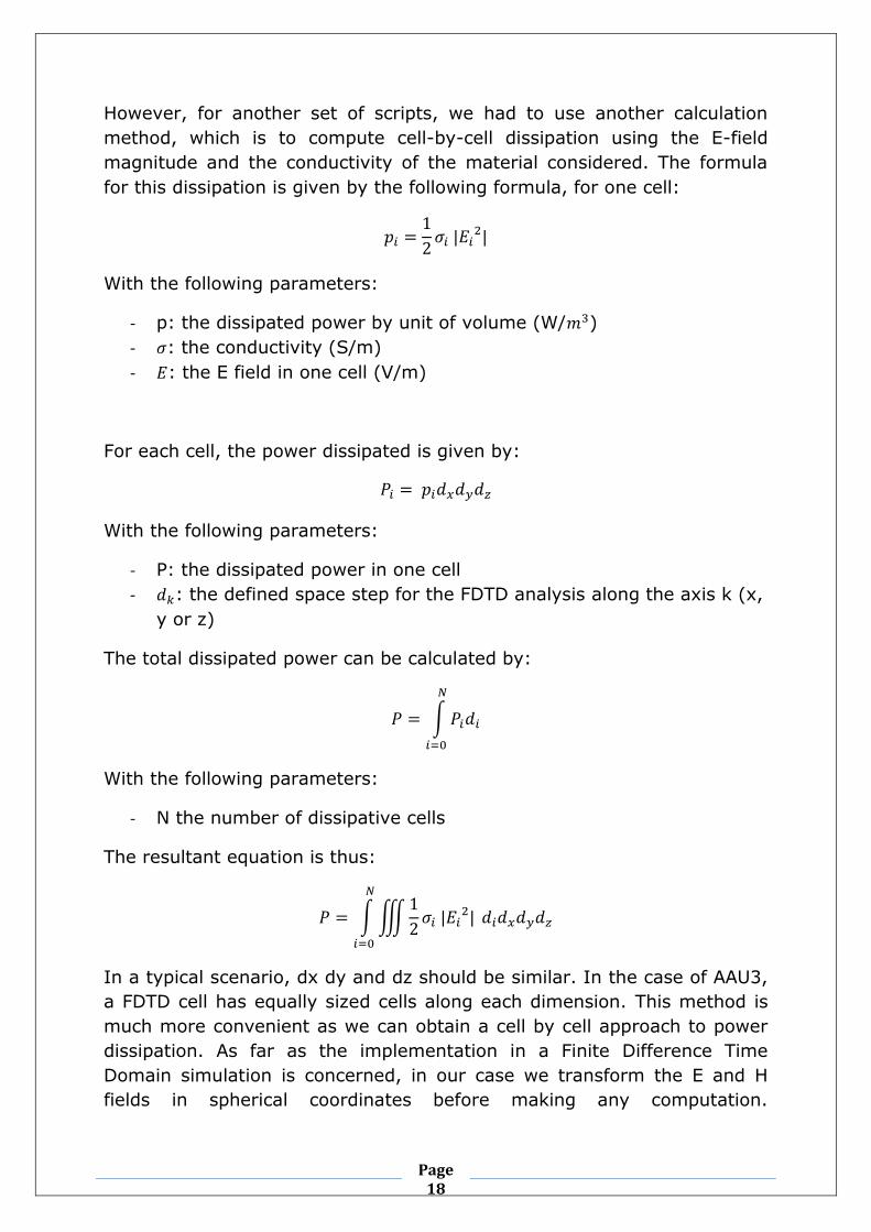
However, for another set of scripts, we had to use another calculation
method, which is to compute cell-by-cell dissipation using the E-field
magnitude and the conductivity of the material considered. The formula
for this dissipation is given by the following formula, for one cell:
With the following parameters:
- p: the dissipated power by unit of volume (W/ )
- : the conductivity (S/m)
- : the E field in one cell (V/m)
For each cell, the power dissipated is given by:
With the following parameters:
- P: the dissipated power in one cell
- : the defined space step for the FDTD analysis along the axis k (x,
y or z)
The total dissipated power can be calculated by:
With the following parameters:
- N the number of dissipative cells
The resultant equation is thus:
In a typical scenario, dx dy and dz should be similar. In the case of AAU3,
a FDTD cell has equally sized cells along each dimension. This method is
much more convenient as we can obtain a cell by cell approach to power
dissipation. As far as the implementation in a Finite Difference Time
Domain simulation is concerned, in our case we transform the E and H
fields in spherical coordinates before making any computation.
Page 19
Page 19
Furthermore, since we only consider a near field simulation, we make use
of the near to far field transformation technique.
2) Total power dissipation
By its nature, power dissipation is one of the key aspects to explore in
order to determine the robustness of an antenna to the human body.
While not really deterministic due to its lack of details, the total power
dissipation does give us an indication about how much an antenna suffers
from the presence of a hand close to it.
Therefore, antennas will be compared to the mean of the total power
dissipated by all antennas and statistics will be shown at the end of
chapter 3. The reference antennas will also be analyzed independently on
this value of total power dissipation.
3) Power dissipation along an axis
A way to obtain a closer look at power dissipation in a brick is to look at it
separately along each axis. The idea behind it being to sum all power
dissipation obtained via the cell by cell power dissipation formula
described above along two axis for one specific value of x,y or z and then
proceed to increment this value.
From this, we can obtain another mean of classification. The one we will
be mostly interested in is the axis intersecting both the ground plane and
the brick (the x axis). Power dissipation along the two first centimeters
along this axis will tell us how much the antenna suffers from the brick
and more importantly, how fast. This power dissipation will be measured
both as a cell by cell graph and as a regrouped by centimeter graph which
provides a greater visibility in terms of relative power dissipation.
Page 20
Page 20
III – Three Dimensional Correlations
1) Cross-correlation definition and explanation
Correlation can be defined as a measure of coherence between to
variables. This meaning that variations within these variables are
measured to grasp how much they behave accordingly. [4]
For one-dimensional variables and since in our case we consider equally
sized variable arrays (as the size of the domain is kept a constant), this
would mean using Pearson’s product-moment equation [5]:
Where represents the value of the variable at a given point, identically
for . In this equation, represents the mean of and the mean of .
and are the sample standard deviation of variables and .
In our case, however, this formula is not sufficient as we consider that a
given variable might also vary in space. Thus creating a need for pattern
recognition which is provided by another correlation method: the cross
correlation.
Cross-correlation is used in several domains like signal processing or
medicine. The idea behind it is to apply a delay to one of the “signals” and
comparing it to the other signal. This method of statistics is used to
recognize tumors on radio scans of patients, for example.
While this method normally applies to different signals, trying to recognize
a smaller one with a bigger one, it also applies for our case as the
radiation pattern might vary between two measurements (with and
without the brick, for example or in the case of different size of domains).
The idea being to measure how much the electromagnetic fields vary
accordingly when confronted with a slight change in the environment, the
introduction of the human hand.
Page 21
Page 21
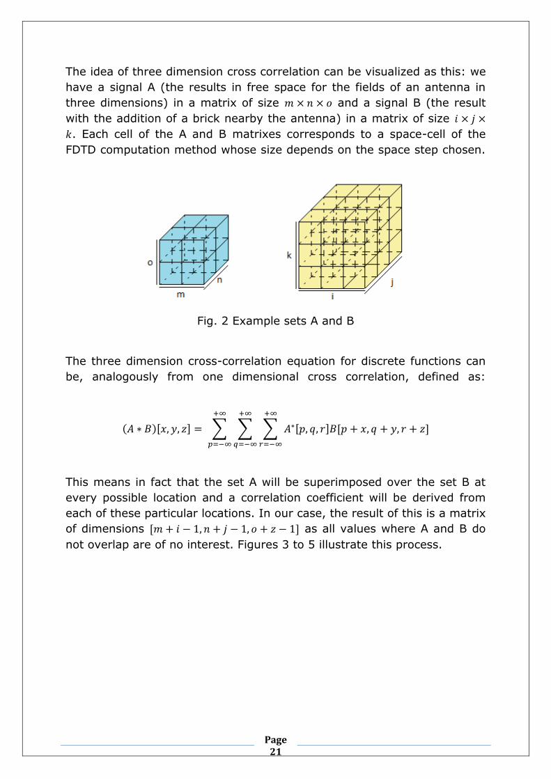
The idea of three dimension cross correlation can be visualized as this: we
have a signal A (the results in free space for the fields of an antenna in
three dimensions) in a matrix of size and a signal B (the result
with the addition of a brick nearby the antenna) in a matrix of size
. Each cell of the A and B matrixes corresponds to a space-cell of the
FDTD computation method whose size depends on the space step chosen.
Fig. 2 Example sets A and B
The three dimension cross-correlation equation for discrete functions can
be, analogously from one dimensional cross correlation, defined as:
This means in fact that the set A will be superimposed over the set B at
every possible location and a correlation coefficient will be derived from
each of these particular locations. In our case, the result of this is a matrix
of dimensions as all values where A and B do
not overlap are of no interest. Figures 3 to 5 illustrate this process.
Page 22
Page 22
Fig. 3 First cross-correlation coefficient computation on overlapping cells
Fig. 4 Second cross-correlation coefficient computation
Fig. 5 Fourth cross-correlation coefficient computation
Then, by transposition on different rows and columns, all matching
possibilities between set A and B are thus explored.
Page 23
Page 23
In our case, there are two possible scenarios for the use of correlation.
Either as described above we simulate a reference antenna in free space
in a small domain then simulate in a wider domain the same antenna with
a brick in its vicinity. The aim of the cross-correlation in this case is to find
a matching E-field pattern inside the wider domain.
The second possibility is a simpler correlation in the case where the size of
the domains in free space and brick simulation are identical. In this case,
to refer to Figures 3 to 5, we only consider the correlation coefficient at
the exact spot where both variable matrixes perfectly match one another.
This second method has given better results and is thus mainly used in
the parts below.
2) Interpretation of results
As the correlation calculation results in a correlation coefficient, it is
important to know how to interpret it. In the case of different-sized
domains and “pattern” recognition, results have shown that very high
correlation coefficients are attained when nearly null electromagnetic
fields are correlated (on the edges for example, when only part of each
set of result overlap).
A correlation coefficient ranks from -1 to +1, depending on the type of
relationship correlating the two variables or, in our case, sets:
- A correlation coefficient of +1 indicates a positive relationship,
meaning that when one variable increases or decreases, so does the
other one.
- A correlation coefficient of -1 indicates a negative or opposite
relationship, meaning that one set of data behaves oppositely to the
other.
- A correlation coefficient of 0 means that there is no link between the
two variables.
- In a general manner, if the absolute value of the correlation
coefficient is above 0.7 it is considered as a high correlation
between the variables, on the other hand absolute values lower than
0.3 indicate a low correlation.
However, correlation does not indicate causality. In our case, this means
that even if an antenna has a very high correlation coefficient between
free space and brick simulations, it does not mean that it is linked to the
Page 24
Page 24
free space simulation. It might however mean that the resistance to the
brick is higher for this antenna.
Let us now proceed to another tool of measurement, the S11 parameter
analysis.
IV – S11 Parameter
To understand the concept of the S11 parameter, let us consider a
transmission line represented by a two-port network where on one end
lays the source and on the other the antenna itself (figure 6).
Fig. 6 A two port network representing a transmission line
The concept of the S11 parameter is simply to represent the reflection
coefficient at the input of the transmission line. What we aim for, with this
parameter, is for it to be the lowest possible at the resonance frequency of
the antenna. Ideally, this would mean a value of 0 but in practice we often
consider that a -10dB is sufficient [6].
The formula for the reflection coefficient is given by:
Where represents the impedance of the transmission line and
represents the impedance at the input of the antenna. To get a perfect
matching (a reflection coefficient with a value of 0), we need to have an
identical value for and .
Page 25
Page 25
The reflection coefficient varies with frequency and can thus have a plot
which looks like the one in figure 7.
Fig. 7 A S11 plot as a function of frequency
From this graph, we can actually obtain much information. First, it is
possible to get the bandwidth by looking at the -6dB values. In figure 7,
for example, the bandwidth is about 0.55 GHz. Secondly, it is also
possible to get the resonant frequency, which in the graph would be
around 7.4 GHz.
The S11 graph is a key tool to see the impact of the hand on an antenna.
Indeed, we are interested by the impact on the bandwidth, but also on the
effect on the resonant frequency and “depth” of the S11 parameter.
V – Imaginary Part
The impedance of an antenna is a complex number, given by the formula
where j is the square root of -1. This impedance has two
components, a real and an imaginary part:
- The real part corresponds to the power radiated or absorbed within
the antenna [7]
- The imaginary part corresponds to the power stored in the reactive
near field of the antenna [7]
We consider there is a resonant frequency where the imaginary part of the
impedance is equal to zero. The imaginary part graph has for purpose to
see how the imaginary part varies with frequency.
Page 26
Page 26
Also, an impedance is said to be inductive when its imaginary part is
negative and capacitive when otherwise [8].
Fig. 8 Imaginary part of a dipole resonating at 1GHz
VI – Smith Chart
The Smith chart is a graph which allows us to represent the impedance
variation of a dipole in function of frequency.
Page 27
Page 27
Fig. 9 Smith Chart
Any impedance, Z= R+jX, can be represented on the Smith Chart. To
determine where an impedance is represented, you have to proceed in
two step.
Firstly, thanks to the real part of the impedance, you can determine on
which constant resistance circle the impedance will be represented[11].
Indeed, each circle, in the smith chart are representing a constant
resistance [9], as we can see on the next scheme:
Page 28
Page 28
Fig. 10 Impedance circles
Each red point, on the previous scheme, has the same resistance (R=0.3),
but they do not have the same imaginary part [12].
The line between the point D and the point F represent all the impedances
with an imaginary part equal to zero.
The point D represents an impedance equal to zero (short circuit). The
point F represents an impedance with an infinite imaginary part (open
line).
Secondly, thanks to the imaginary part, you can determine on which
constant reactance circle the impedance will be represented.
These constant reactance circles are represented on the next scheme:
Page 29
Page 29
Fig. 11 Imaginary parts
Each blue points, on the previous scheme, has the same reactance (X=-
0.4), but they don’t have the same real part.
All the inductive reactance (X>0) are in red on the previous scheme, and
the capacitive reactance (X<0) are in blue.
We can notice that the circle corresponding to Z=0, in green on the next
scheme, which is the normalized Smith Chart[10].
Fig. 12 Impedance axes
With this normalized Smith Chart, each part of the impedance must be
divided by the characteristic impedance Z0 of the transmission line. The
representation uses the normalized impedance.
For example, the representation of the normalized impedance
Z=0.3+0.4j, is on the next graph:
Page 30
Page 30
Fig. 13 Total impedance
The reflection coefficient is
with the characteristic
impedance can be read on the Smith Chart. It’s given by the line between
the point representing the impedance, and the center of the Smith chart (
R=1 and X=0). Indeed, the smith chart is the representation of the
reflection coefficient in polar coordinates.
Fig. 14 Reflection coefficient at the transmission line
Page 31
Page 31
The scale around the smith chart represents the wavelength but also the
angle of the reflection coefficient:
Fig 15. Wavelength scale
So, we are able, thanks to the Smith chart, to have the reflection
coefficient in function of frequency. In conclusion, the smith chart can be
used to solve matching problems.
VI – Finding the appropriate brick
One of the most important aspects of this research was to define a
reference brick that could be used by telecommunications engineers to
simulate the impact of the human hand on the quality of their antenna
design. In order to achieve this reference brick, a certain number of
assertions had to be made:
- As the design was to be as simple as possible, we considered the
hand as a single layer object, so we did not consider the bone, flesh
or fat’s particular impact on power dissipation. However, this was
the topic of a side experiment described in the chapter below.
- We had acquired an AAU3-compatible design (figure 16) for the
human hand from the PhD of Mauro Pelosi, our supervisor, which we
tried so make simpler. [1]
Page 32
Page 32
Fig. 16 An AAU3 human hand design
The key factor for the acceptation of the reference brick that would
become our human hand proxy was that the total power dissipated was
identical between the brick and the hand. This simplification has limits, of
course, as the power dissipated calculated along the axes is of course a
very rough estimation.
The hand being rather thin (from 1 to 3 centimeters at maximum), the
brick should also not be cubic but rather thin. In the end, we did find a
brick corresponding to these different criterions (show in fig 17) with
parameters of permittivity=36.2, conductivity=0.79 and permeability=1.
Fig. 17 The simplified human hand model
Page 33
Page 33
CHAPTER TWO: SIDE EXPERIMENTS
Aside from the main experiment about the determination of a robustness
criterion, we have pushed our research into several sub-areas related to
the topic based on references we read to understand the topic or simply to
determine as accurately as possible the way the tools described above
would be used.
I – Conductivity, permittivity and
permeability variations
The human hand is composed of several layers (fat, skin, bone, flesh et
cetera) which have distinct values for conductivity (the ability to conduct
current), permittivity (the measure of resistance to electric field
formation) and permeability (the degree of magnetization of a material in
response to a magnetic field).
The purpose of this experiment was to determine the impact of these
three parameters on the power dissipation of the fields within these
modified mediums.
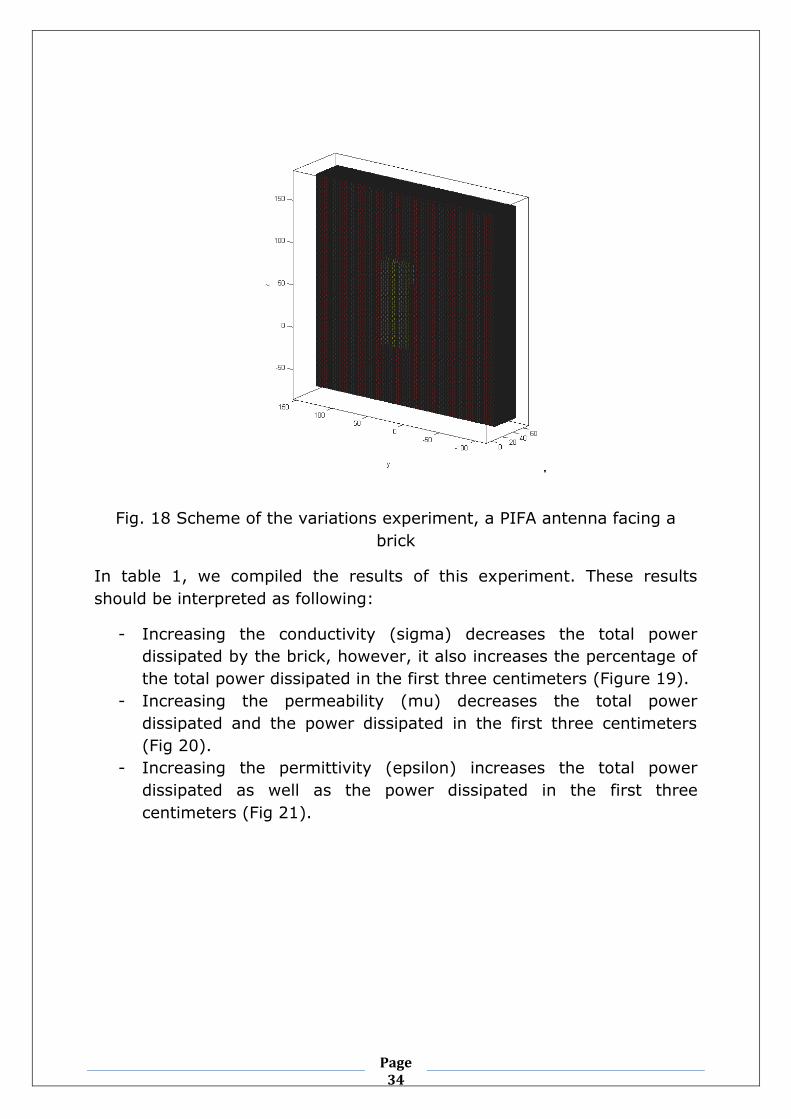
In order to do so, we consider a PIFA antenna and a brick of 40x250x250
millimeters at the distance of 30 millimeters from the antenna and we
consider the rest of the medium to be free space. Figure 18 below shows
the layout of the experiment.
As for results, we consider power dissipation along three separate axes as
described in the power dissipation chapter. However, we were only
interested by the x-axis power dissipation in the first three centimeters.
Page 34
Page 34
Fig. 18 Scheme of the variations experiment, a PIFA antenna facing a
brick
In table 1, we compiled the results of this experiment. These results
should be interpreted as following:
- Increasing the conductivity (sigma) decreases the total power
dissipated by the brick, however, it also increases the percentage of
the total power dissipated in the first three centimeters (Figure 19).
- Increasing the permeability (mu) decreases the total power
dissipated and the power dissipated in the first three centimeters
(Fig 20).
- Increasing the permittivity (epsilon) increases the total power
dissipated as well as the power dissipated in the first three
centimeters (Fig 21).
Page 35
Page 35
Sigma Mu Epsilon Pdis C by C Pdis < 3cm % of total
0,85 1 42,5 8,34E-10 7,10E-10 85,11
1 1 42,5 8,52E-10 7,47E-10 87,68
2 1 42,5 8,05E-10 7,79E-10 96,75
3 1 42,5 7,11E-10 7,04E-10 98,92
4 1 42,5 6,34E-10 6,30E-10 99,44
1 1 1 1,04E-09 1,02E-09 97,80
1 1 1,5 1,05E-09 1,03E-09 97,71
1 1 2 1,06E-09 1,03E-09 97,61
1 1 10 1,11E-09 1,06E-09 95,65
1 1 20 1,05E-09 9,74E-10 92,71
1 1 30 9,04E-10 8,13E-10 90,00
1 2 42,5 1,10E-09 1,02E-09 93,05
1 4 42,5 1,48E-09 1,43E-09 96,74
Table 1 Results of the variations experiment
Fig. 19 Relative power dissipation according to the variation of sigma
75,00
80,00
85,00
90,00
95,00
100,00
105,00
0,85 1 2 3 4
% of power dissipated Mu=1, Eps=42.5
Page 36
Page 36
Fig. 20 Relative power dissipation according to the variations of epsilon
Fig. 21 Relative power dissipation according to the variation of mu
In the same manner, some results have shown that the repartition of
power dissipation varies a great deal when varying parameters as shown
in figures 22-23 below.
86,00
88,00
90,00
92,00
94,00
96,00
98,00
100,00
1 1,5 2 10 20 30
% of power dissipated Mu=1, Sig=1
82,00
84,00
86,00
88,00
90,00
92,00
94,00
96,00
98,00
1 2 4
% of power dissipated Sig=1, Eps=42.5
Page 37
Page 37
Fig. 22 Power dissipation along the x-axis with a permeability of 42.5
Fig. 23 Power dissipation along the x-axis with a permeability of 1.5
While in the end we considered the hand as a homogeneous brick with
parameters of mu =1, sigma =0.79 and epsilon = 36.2, this research has
raised some interesting questions about the impact of these parameters
on the agglomeration or not of the total power dissipation at one end of
the brick.
Page 38
Page 38
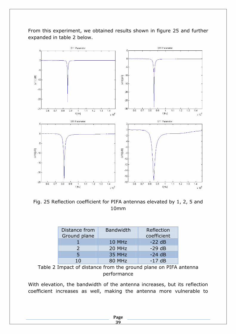
II – Narrowband PIFA study
One of the antennas we decided to include as our reference antennas was
the narrowband PIFA antenna, for which we aimed to resonate at a
frequency of 850MHz (UMTS V). We decided to look at the impact of
bringing the antenna closer to the ground plane as a matter of reflection
coefficient and bandwidth. Our reference PIFA antenna was separated
from the ground plane by 10 millimeters, and this study used distances of
1, 2 and 5 millimeters to witness the impact of this distance.
Fig. 24 PIFA antennas separated by 1, 2, 5 and 10mm from the ground
plane
Page 39
Page 39
From this experiment, we obtained results shown in figure 25 and further
expanded in table 2 below.
Fig. 25 Reflection coefficient for PIFA antennas elevated by 1, 2, 5 and
10mm
Distance from
Ground plane
Bandwidth Reflection
coefficient
1 10 MHz -22 dB
2 20 MHz -29 dB
5 35 MHz -24 dB
10 80 MHz -17 dB
Table 2 Impact of distance from the ground plane on PIFA antenna
performance
With elevation, the bandwidth of the antenna increases, but its reflection
coefficient increases as well, making the antenna more vulnerable to
Page 40
Page 40
interference. For the robustness experiment, a 1mm PIFA narrowband
antenna was used.
III – Impact of the permittivity of the
substrate on a thin substrate-layered PIFA
antenna
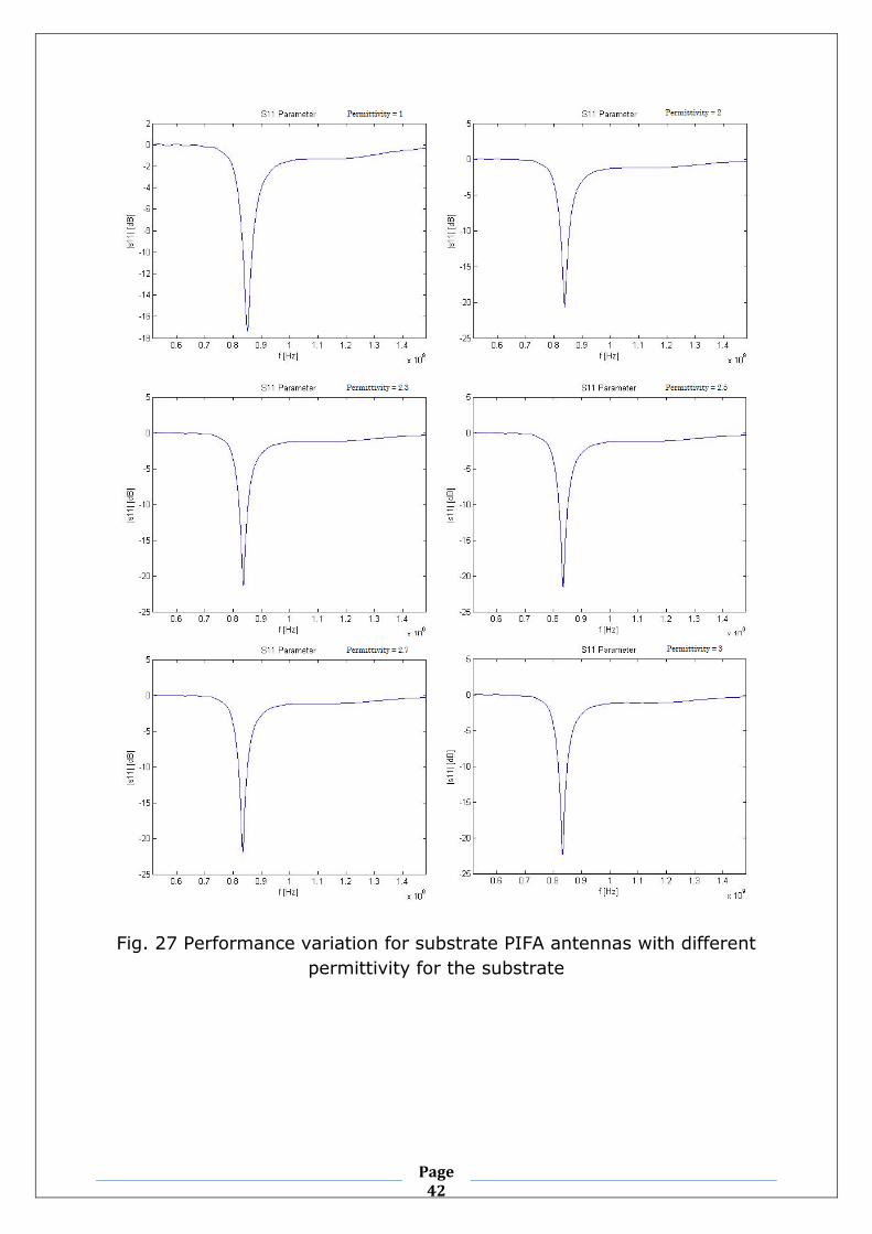
One of the reference antennas considered was the PIFA with substrate,
one of the first designs was a thin layer of substrate directly imposed on
the PIFA antenna. As several substrates are available, a quick study was
made on the impact of a change of permittivity of the substrate on the
performance of the antenna. The antenna design can be seen in figure 26
below.
Fig. 26 Thin-layered substrate PIFA antenna
The considered values of permittivity were 1, 2, 2.3, 2.5, 2.7 and 3 F/m.
Results of this experiment are shown in figure 27 below and expanded in
table 3.
Page 41
Page 41
Permittivity Resonance frequency
Bandwidth Reflection coefficient
1 850 MHz 60 MHz -17 dB
2 830 MHz 50 MHz -20 dB
2.3 830 MHz 40 MHz -22 dB
2.5 830 MHz 35 MHz -23 dB
2.7 830 MHz 30 MHz -23 dB
3 830 MHz 25 MHz -23 dB
Table 3 Performance variation of a thin-layered substrate PIFA antenna
with a change of permittivity of the substrate
The conclusion of this study is that when increasing the permittivity of the
substrate, the reflection coefficient decreases to a minimum (in our case
of -23 dB), the resonance frequency varies little and more importantly,
the bandwidth decreases with the increase of permittivity. In the case of
the substrate PIFA reference antenna used for robustness simulations, a
permittivity of 1 F/m was chosen.
Page 42
Page 42
Fig. 27 Performance variation for substrate PIFA antennas with different
permittivity for the substrate
Page 43
Page 43
IV – Defining the composition of the
human hand
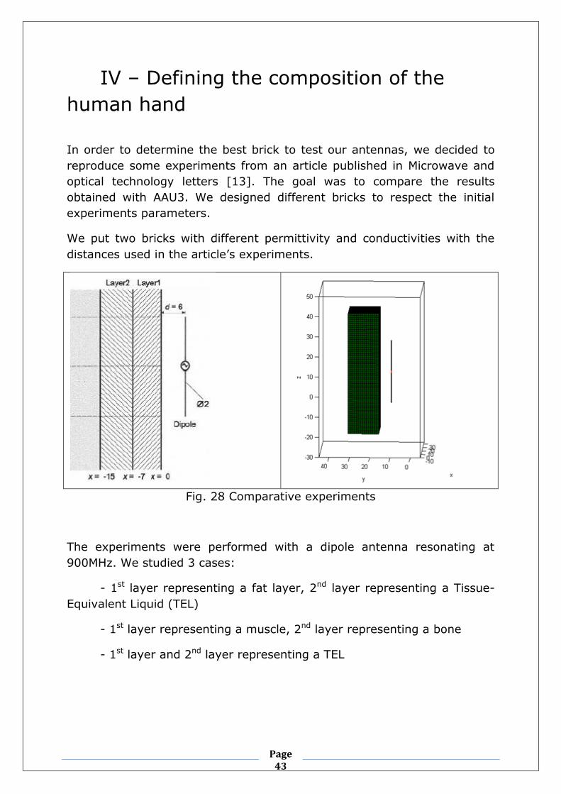
In order to determine the best brick to test our antennas, we decided to
reproduce some experiments from an article published in Microwave and
optical technology letters [13]. The goal was to compare the results
obtained with AAU3. We designed different bricks to respect the initial
experiments parameters.
We put two bricks with different permittivity and conductivities with the
distances used in the article’s experiments.
Fig. 28 Comparative experiments
The experiments were performed with a dipole antenna resonating at
900MHz. We studied 3 cases:
- 1st layer representing a fat layer, 2nd layer representing a Tissue-
Equivalent Liquid (TEL)
- 1st layer representing a muscle, 2nd layer representing a bone
- 1st layer and 2nd layer representing a TEL
Page 44
Page 44
Material permittivity conductivity
Tissue-Equivalent Liquid (TEL)
42.50 0.850
Muscle 55.95 0.969
Bone 16.62 0.242
Fat 5.00 0.025
Table 4 Values of specific hand components
What we were concerned in these simulations was the E field magnitude.
In figures below, the results are presented
Fig. 29 1st layer representing a fat layer, 2nd layer representing a Tissue-
Equivalent Liquid (TEL)
Page 45
Page 45
Fig. 30 1st layer representing a muscle, 2nd layer representing a bone
Fig. 31 1st layer and 2nd layer representing a TEL
Page 46
Page 46
With the different tools of AAU3, we were able to have some precise
measures for the E field. Unfortunately, we were not able to compare
precisely our results with those of the article [14]. For example, our
comparison graph for the 3rd case is shown in figure 32 below.
Fig. 32 Paper results
While recreating the results of this paper has revealed itself of no use for
our own problem, it was still a pertinent insight on the importance of the
nature of the hand and the composition of its simulated alter ego.
Page 47
Page 47
CHAPTER THREE: SIMULATION
PARADIGM AND ALTERATION
I – Introduction
As described in the introduction, we used for this project a Finite
Difference Time Domain approach to the computation of fields near our
antennas. This FDTD analysis was made possible via the AAU3 software, a
Matlab based software allowing us to design antennas and simulate their
theoretical fields and such in a very customizable manner [15].
Furthermore, this software allowed us to design objects with specific
parameters (like the hand or just a brick) to be put close to the antenna.
While this program has been at the center of our simulation environment,
it turns out a few changes needed to be made to the code in order for us
to obtain the best possible results. Notably, this is what made us to a
slicer to visualize three dimensional fields more clearly than what AAU3
offered, but not only. Indeed, with the use of two separate power
dissipation calculation techniques, results have shown that there is a
difference between the power dissipated results of these two methods.
Eventually, the changes brought to the software will be described.
II – Slicer
The AAU3 program being able to compute electromagnetic fields in three
dimensions, it seems obvious that a pertinent graphic approach to the
results be set in place. However, the basic AAU3 software did not possess
a convenient way to visualize these fields (figure 33), as having to set a
cursor on three different graphs to see a result was not very satisfying.
So, in order to have a more graphic result, we programmed a script which
Page 48
Page 48
shows along an axis a “slice” of the three dimensional results matrix. That
way, the fields were much easier to witness (figure 34).
Fig. 33 Regular field graph
Fig. 34 Slicer
III – Difference in power calculation
As described in chapter two, there are two methods of calculation for the
total power dissipated. One approach, used by the AAU3 software, is via
the computation of the pointing vector. The other is a more down-to-earth
method, the summation of the power dissipation of each cell.
While using both techniques in our simulations, we realized that the
results were not identical, which led to some questioning about whether
Page 49
Page 49
one or the other technique was not correctly implemented. However, it
turned out that both were correct, so we did some research to see if this
error could be predicted. Using the same simulation as the “Conductivity,
permittivity and permeability variations” side experiment, we obtained the
results in table 4 below.
Sigma Mu Epsilon Pdis C by C
Pdis AAU3 %Err
0,85 1 42,5 8,34E-10 8,53E-10 2,24
1 1 42,5 8,52E-10 8,71E-10 2,22
2 1 42,5 8,05E-10 8,27E-10 2,65
3 1 42,5 7,11E-10 7,36E-10 3,33
4 1 42,5 6,34E-10 6,59E-10 3,82
1 1 1 1,04E-09 1,07E-09 2,74
1 1 1,5 1,05E-09 1,08E-09 2,72
1 1 2 1,06E-09 1,09E-09 2,69
1 1 10 1,11E-09 1,14E-09 2,44
1 1 20 1,05E-09 1,07E-09 2,18
1 1 30 9,04E-10 9,24E-10 2,21
1 2 42,5 1,10E-09 1,12E-09 2,26
1 4 42,5 1,48E-09 1,52E-09 2,68
Table 5 Error calculation between computation techniques
While the error is always small, it seems as though the smaller the total
power dissipation was, the higher the error was. This made us think that
there might be a “static” error overcome with large numbers. However,
we could not prove this hypothesis.
IV – Changes brought to AAU3
The main alteration we had to bring to AAU3 concerned the exportation of
parameters and files. As such, we have made the exportation of results
systematic and computation of fields and such automatic as well. Finally,
we developed some scripts to compute the power dissipation or even
show it right after computation by AAU3.
Page 50
Page 50
CHAPTER FOUR: COMPARISON OF
REFERENCE ANTENNAS
I – Introduction
Now that we have defined the different lenses under which the antennas
will be analyzed, let us introduce the simulation results and an
interpretation on each of these results. Every antenna will first be
compared to itself in free space, but with a brick close-by. Then, in the
next chapter, all antennas will be compared to one another.
In this chapter, antennas will be described by a certain number of graphs
or data:
- Actual graph of the antenna
- S11 graph
- Imaginary part graph
- Smith chart
- 3D correlation coefficient
- Power dissipated along axes
- Total power dissipated
- Antenna efficiency
Page 51
Page 51
II – Dipole
The actual design of the antenna:
Fig. 35 A free space dipole antenna design
Fig. 36 A brick close by the dipole
Page 52
Page 52
The comparative S11 graphs:
Fig. 37 Free space S11 for a dipole antenna
Fig. 38 Brick S11 for a dipole antenna
Page 53
Page 53
Imaginary parts of the dipole:
Fig. 39 Imaginary part of a free space dipole
Fig. 40 Brick imaginary part of a dipole
Page 54
Page 54
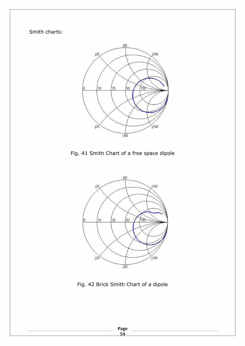
Smith charts:
Fig. 41 Smith Chart of a free space dipole
Fig. 42 Brick Smith Chart of a dipole
Page 55
Page 55
Power dissipation along x:
Fig. 43 Power dissipated along axis X for a dipole
Numerical indicators:
- 3D Correlation coefficient 9.3818471e-01
- Total power dissipated 4.8250443e-09
- Power dissipated in the first 1.1cm 2.9959556e-09
- In percentage of total power dissipated 62.091774%
- Antenna efficiency without brick 0.98655
- Antenna efficiency with brick 0.32928
Page 56
Page 56
III – Monopole
The actual design of the antenna:
Fig. 44 The free space design of a monopole
Fig. 45 The brick design of a monopole
Page 57
Page 57
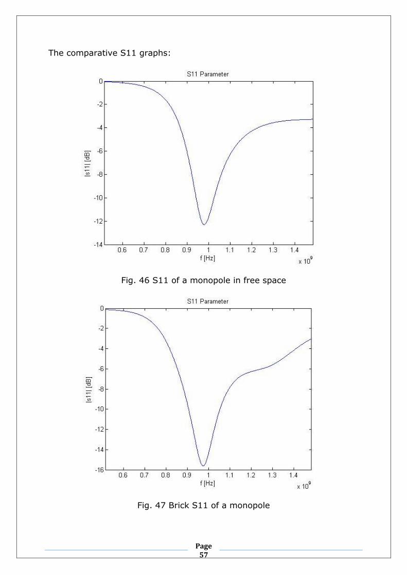
The comparative S11 graphs:
Fig. 46 S11 of a monopole in free space
Fig. 47 Brick S11 of a monopole
Page 58
Page 58
Imaginary parts of the monopole:
Fig. 48 Imaginary part of a free space monopole
Fig. 49 Brick imaginary part of a monopole
Page 59
Page 59
Smith Charts:
Fig. 50 Smith Chart for a free space monopole
Fig. 51 Brick Smith Chart for a monopole
Page 60
Page 60
Power dissipation along x:
Fig. 52 Power dissipated along x for a monopole
Numerical indicators:
- 3D Correlation coefficient 8.8779460e-01
- Total power dissipated 5.2063101e-09
- Power dissipated in the first 1.1cm 2.9341756e-09
- In percentage of total power dissipated 56.358065%
- Antenna efficiency without brick 0.98757
- Antenna efficiency with brick 0.31217
Page 61
Page 61
IV – PIFA
The actual design of the antenna:
Fig. 53 The free space design of a PIFA
Fig. 54 The brick design of a PIFA
Page 62
Page 62
The comparative S11 graphs:
Fig. 55 S11 of a PIFA in free space
Fig. 56 Brick S11 of a PIFA
Page 63
Page 63
Imaginary parts of the PIFA:
Fig. 57 Imaginary part of a free space PIFA
Fig. 58 Brick imaginary part of a PIFA
Page 64
Page 64
Smith Charts:
Fig. 59 Smith Chart for a free space PIFA
Fig. 60 Brick Smith Chart for a PIFA
Page 65
Page 65
Power dissipation along x:
Fig. 61 Power dissipation along x for a PIFA
Numerical indicators:
- 3D Correlation coefficient 7.7953279e-01
- Total power dissipated 1.9273124e-09
- Power dissipated in the first 1.1cm 1.0463317e-09
- In percentage of total power dissipated 54.289677%
- Antenna efficiency without brick 0.99398
- Antenna efficiency with brick 0.48337
Page 66
Page 66
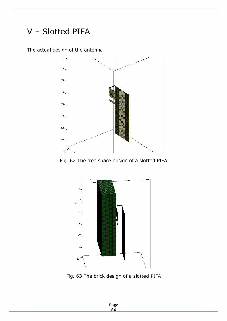
V – Slotted PIFA
The actual design of the antenna:
Fig. 62 The free space design of a slotted PIFA
Fig. 63 The brick design of a slotted PIFA
Page 67
Page 67
The comparative S11 graphs:
Fig. 64 S11 of a slotted PIFA in free space
Fig. 65 Brick S11 of a slotted PIFA
Page 68
Page 68
Imaginary parts of the slotted PIFA:
Fig. 66 Imaginary part of a free space slotted PIFA
Fig. 67 Brick imaginary part of a slotted PIFA
Page 69
Page 69
Smith Charts:
Fig. 68 Smith Chart for a free space slotted PIFA
Fig. 69 Brick Smith Chart for a slotted PIFA
Page 70
Page 70
Power dissipation along x:
Fig. 70 Power dissipation along x for a slotted PIFA
Numerical indicators:
- 3D Correlation coefficient 8.2940498e-01
- Total power dissipated 9.2544406e-10
- Power dissipated in the first 1.1cm 4.7393127e-10
- In percentage of total power dissipated 51.211228%
- Antenna efficiency without brick 0.98656
- Antenna efficiency with brick 0.39744
Page 71
Page 71
VI – Narrowband PIFA
The actual design of the antenna:
Fig. 71 The free space design of a narrowband PIFA antenna
Fig. 72 The brick design of a narrowband PIFA antenna
Page 72
Page 72
The comparative S11 graphs:
Fig. 73 S11 of a narrowband PIFA antenna in free space
Fig. 74 Brick S11 of a narrowband PIFA antenna
Page 73
Page 73
Imaginary parts of the narrowband PIFA antenna:
Fig. 75 Imaginary part of a free space narrowband PIFA antenna
Fig. 76 Brick imaginary part of a narrowband PIFA antenna
Page 74
Page 74
Smith Charts:
Fig. 77 Smith Chart for a free space narrowband PIFA antenna
Fig. 78 Brick Smith Chart for a narrowband PIFA antenna
Page 75
Page 75
Power dissipation along x:
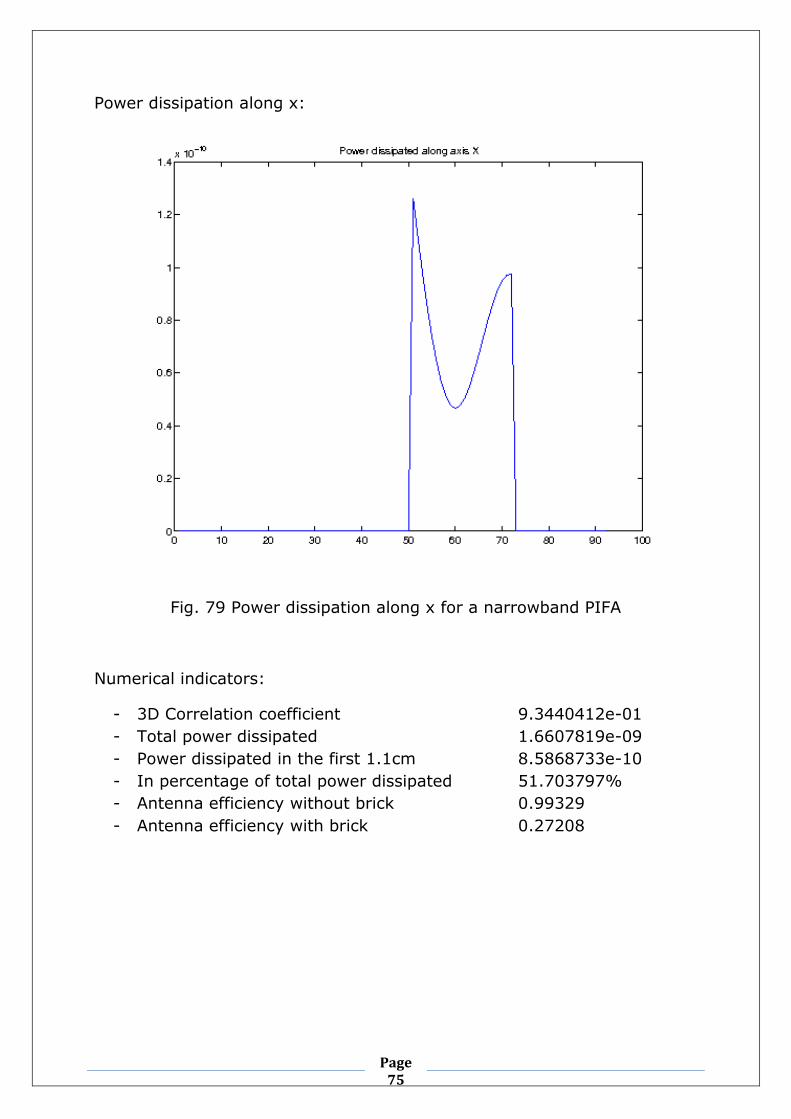
Fig. 79 Power dissipation along x for a narrowband PIFA
Numerical indicators:
- 3D Correlation coefficient 9.3440412e-01
- Total power dissipated 1.6607819e-09
- Power dissipated in the first 1.1cm 8.5868733e-10
- In percentage of total power dissipated 51.703797%
- Antenna efficiency without brick 0.99329
- Antenna efficiency with brick 0.27208
Page 76
Page 76
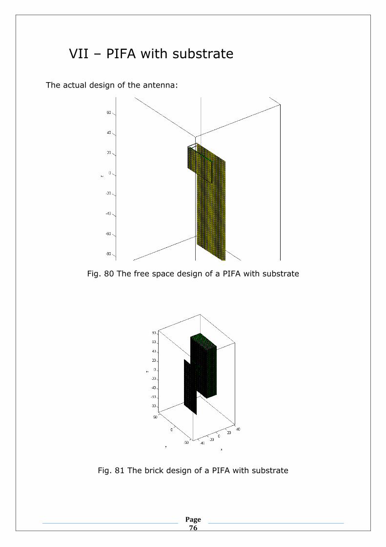
VII – PIFA with substrate
The actual design of the antenna:
Fig. 80 The free space design of a PIFA with substrate
Fig. 81 The brick design of a PIFA with substrate
Page 77
Page 77
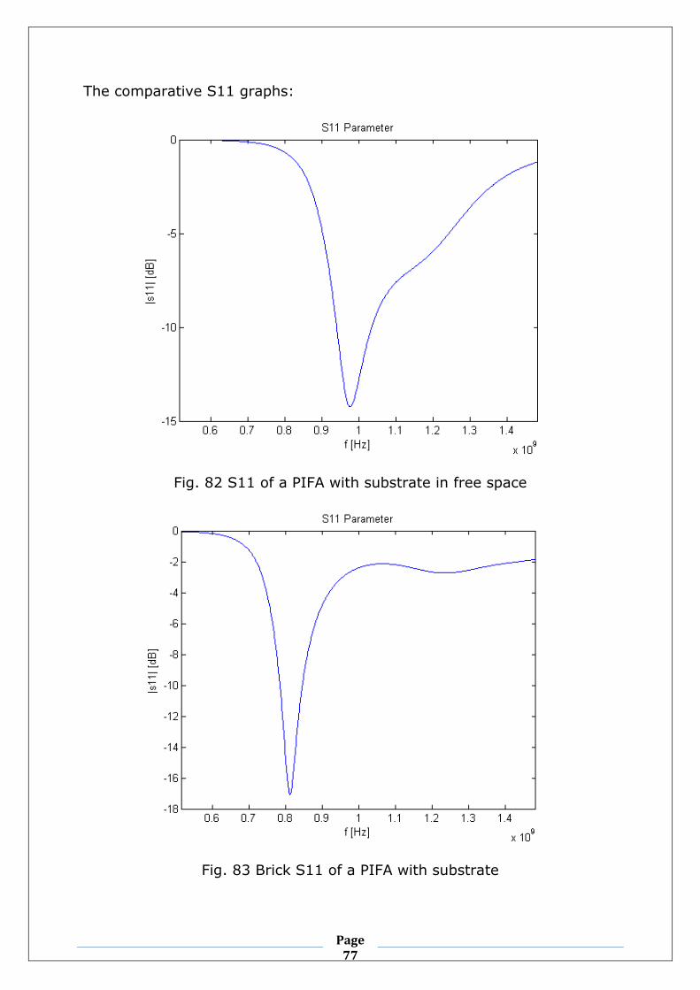
The comparative S11 graphs:
Fig. 82 S11 of a PIFA with substrate in free space
Fig. 83 Brick S11 of a PIFA with substrate
Page 78
Page 78
Imaginary parts of the PIFA with substrate:
Fig. 84 Imaginary part of a free space PIFA with substrate
Fig. 85 Brick imaginary part of a PIFA with substrate
Page 79
Page 79
Smith Charts:
Fig. 86 Smith Chart for a free space PIFA with substrate
Fig. 87 Brick Smith Chart for a PIFA with substrate
Page 80
Page 80
Power dissipation along x:
Fig. 88 Power dissipation along x for a PIFA with substrate
Numerical indicators:
- 3D Correlation coefficient 7.8212312e-01
- Total power dissipated 1.7478407e-09
- Power dissipated in the first 1.1cm 9.1430834e-10
- In percentage of total power dissipated 52.310736%
- Antenna efficiency without brick 0.95965
- Antenna efficiency with brick 0.4699
Page 81
Page 81
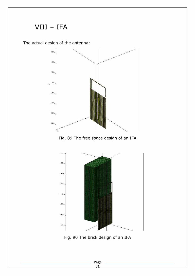
VIII – IFA
The actual design of the antenna:
Fig. 89 The free space design of an IFA
Fig. 90 The brick design of an IFA
Page 82
Page 82
The comparative S11 graphs:
Fig. 91 S11 of an IFA in free space
Fig. 92 Brick S11 of an IFA
Page 83
Page 83
Imaginary parts of the IFA:
Fig. 93 Imaginary part of a free space IFA
Fig. 94 Brick imaginary part of an IFA
Page 84
Page 84
Smith Charts:
Fig. 95 Smith Chart for a free space IFA
Fig. 96 Brick Smith Chart for an IFA
Page 85
Page 85
Power dissipation along x:
Fig. 97 Power dissipation along x for an IFA
Numerical indicators:
- 3D Correlation coefficient 8.9221447e-01
- Total power dissipated 4.4539315e-09
- Power dissipated in the first 1.1cm 2.3802706e-09
- In percentage of total power dissipated 53.442012%
- Antenna efficiency without brick 0.9834
- Antenna efficiency with brick 0.12459
Page 86
Page 86
IX – Loop
The actual design of the antenna:
Fig. 98 The free space design of a loop
Fig. 99 The brick design of a loop
Page 87
Page 87
The comparative S11 graphs:
Fig. 100 S11 of a loop in free space
Fig. 101 Brick S11 of a loop
Page 88
Page 88
Imaginary parts of the loop:
Fig. 102 Imaginary part of a free space loop
Fig. 103 Brick imaginary part of a loop
Page 89
Page 89
Smith Charts:
Fig. 104 Smith Chart for a free space loop
Fig. 105 Brick Smith Chart for a loop
Page 90
Page 90
Power dissipation along x:
Fig. 106 Power dissipation along x for a loop antenna
Numerical indicators:
- 3D Correlation coefficient 9.7498478e-01
- Total power dissipated 2.8384263e-09
- Power dissipated in the first 1.1cm 1.6093313e-09
- In percentage of total power dissipated 56.698011%
- Antenna efficiency without brick 0.92281
- Antenna efficiency with brick 0.45792
Page 91
Page 91
X – Folded loop
The actual design of the antenna:
Fig. 107 The free space design of a folded loop
Fig. 108 The brick design of a folded loop
Page 92
Page 92
The comparative S11 graphs:
Fig. 109 S11 of a folded loop in free space
Fig. 110 Brick S11 of a folded loop
Page 93
Page 93
Imaginary parts of the folded loop:
Fig. 111 Imaginary part of a free space folded loop
Fig. 112 Brick imaginary part of a folded loop
Page 94
Page 94
Smith Charts:
Fig. 113 Smith Chart for a free space folded loop
Fig. 114 Brick Smith Chart for a folded loop
Page 95
Page 95
Power dissipation along x:
Fig. 115 Power dissipation along x for a folded loop antenna
Numerical indicators:
- 3D Correlation coefficient 8.5352060e-01
- Total power dissipated 1.5518543e-09
- Power dissipated in the first 1.1cm 8.3166922e-10
- In percentage of total power dissipated 53.591967%
- Antenna efficiency without brick 0.99661
- Antenna efficiency with brick 0.21347
Page 96
Page 96
CHAPTER FIVE: PARAMETERISATION
AND ROBUSTNESS CRITERION
In this chapter, we will present the results of our different calculations and
the antenna ranking in term of robustness established from them.
I – Percentage of power dissipated
Using a Matlab script, we have determined the quantity of power which
has been dissipated in the “test brick”. We have then made a ratio of this
quantity over the input power to classify the antennas regarding the fact
that they lose the less power as possible inside the brick.
Here is a sum-up table of the results:
Dissipated power (W) Input Power (W) Dissipated power (%)
Loop 2,84E-09 5,63E-09 50,38%
PIFA 1,93E-09 3,73E-09 51,63%
PIFA with substrate 1,75E-09 3,33E-09 52,43%
Slotted PIFA 9,25E-10 1,57E-09 58,80%
Dipole 4,83E-09 7,18E-09 67,21%
Monopole 5,21E-09 7,56E-09 68,84%
Narrowband PIFA 1,66E-09 2,29E-09 72,51%
Folded loop 1,55E-09 1,97E-09 78,59%
IFA 4,45E-09 5,09E-09 87,46%
Table 6 Power dissipated for the different antennas
According to this method, the best antenna is the loop antenna.
Page 97
Page 97
II – 3D Correlation of E-fields
This method consists of a normalized cross correlation in three dimensions
between the electric fields of the simulation of the antenna in free space
and the electric fields obtained from the simulation of the antenna with
the test brick. This way, we measure how much the fields are altered by
the brick.
We have based the Matlab script on the function “normxcorr3” developed
by Daniel Eaton, initially made for some medical imaging purposes and
which is derived from the Matlab “normxcorr2” function.
The following table sums up the results obtained:
3D-Correlation
Loop 97,50%
Dipole 93,82%
Narrowband PIFA 93,44%
IFA 89,22%
Monopole 88,78%
Folded loop 85,35%
Slotted PIFA 82,94%
PIFA with substrate 78,21%
PIFA 77,95%
Table 7 3D-correlation coefficients
According to this method, the antenna which produces electric fields the
least affected by the brick is the loop antenna.
III – General shape evaluation
In order to classify the antenna based on the graphical representation of
the S11 parameters, we firstly decided to make a cross correlation
between the data of the s11 obtained in free space and the ones from the
s11 obtained with the test brick.
The results we have obtained are listed on the following table:
Page 98
Page 98
Cross-correlation
Slotted PIFA 0,996
Narrowband PIFA 0,987
Monopole 0,978
Folded loop 0,966
Loop 0,947
Dipole 0,658
PIFA 0,521
PIFA with substrate -0,266
IFA -0,464
Table 8 Cross-correlation coefficients of S11 curves
Unfortunately, these results didn’t appear to be really accurate. This is
why we have decided to proceed to a visual comparison of the different
graphs and then establish a ranking based on the impact on the shape.
The following figures represent the comparison of the S11 in free space
and with the brick for every antenna:
Fig. 116 Comparison of the S11 parameters for the dipole antenna
Page 99
Page 99
Fig. 117 Comparison of the S11 parameters for the folded loop antenna
Fig. 118 Comparison of the S11 parameters for the IFA antenna
Page 100
Page 100
Fig. 119 Comparison of the S11 parameters for the loop antenna
Fig. 120 Comparison of the S11 parameters for the monopole antenna
Page 101
Page 101
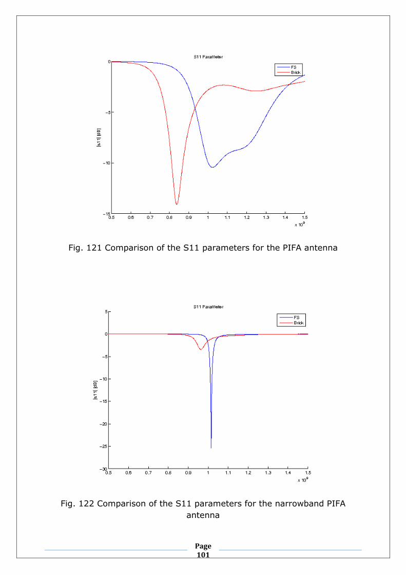
Fig. 121 Comparison of the S11 parameters for the PIFA antenna
Fig. 122 Comparison of the S11 parameters for the narrowband PIFA
antenna
Page 102
Page 102
Fig. 123 Comparison of the S11 parameters for the slotted PIFA antenna
Fig. 124 Comparison of the S11 parameters for the PIFA with substrate
antenna
Page 103
Page 103
For this visual method, the ranking is now as follows (from the best to the
worst antenna):
Monopole
Dipole
Loop
Slotted PIFA
IFA
Folded loop
PIFA with substrate
PIFA
Narrowband PIFA
Table 9 Visual ranking
IV – Variation of the resonant frequency
and the associated S11 parameter
Firstly, we have decided to evaluate the variation of the resonant
frequency calculated by the AAU3 software between the free space
simulations and the simulations with a brick.
The following table sums up the results:
Free space freq. (Hz) Brick freq. (Hz) Variation (Hz)
Monopole 9,80E+08 9,85E+08 5,00E+06
Dipole 9,94E+08 9,63E+08 3,10E+07
Loop 9,97E+08 9,56E+08 4,10E+07
Narrowband PIFA 1,02E+09 9,63E+08 5,20E+07
IFA 1,02E+09 9,13E+08 1,02E+08
Folded loop 8,86E+08 7,64E+08 1,22E+08
Slotted PIFA 9,93E+08 8,42E+08 1,51E+08
PIFA with substrate 9,85E+08 8,12E+08 1,73E+08
PIFA 1,02E+09 8,38E+08 1,85E+08
Table 10 Resonant frequencies for the different antennas
Page 104
Page 104
We have then evaluated the variation of the S11 at the resonant
frequency:
S11 FS (dB) S11 brick (dB) Variation (dB)
Loop -7,49 -7,42 0,07
Dipole -14,92 -14,00 0,92
Monopole -12,30 -15,35 3,05
PIFA with substrate -13,97 -17,07 3,10
PIFA -10,45 -14,11 3,66
IFA -17,13 -8,02 9,12
Slotted PIFA -25,88 -13,37 12,51
Folded loop -11,14 -29,69 18,55
Narrowband PIFA -25,37 -3,44 21,93
Table 11 S11 variations
The loop antenna is the antenna which his having the smallest variation of
the s11.
V – Evolution of the Efficiency
Here are the results compiled from AU3 and showing the evolution of the
efficiency in case of a free space simulation or with the brick. The
antennas have been ranked according to the variation of this efficiency
(the smaller, the better):
Efficiency FS Efficiency brick Variation
Loop 0,9228 0,4579 50,38%
PIFA 0,9940 0,4834 51,37%
PIFA with substrate 0,9597 0,4610 51,96%
Slotted PIFA 0,9866 0,3974 59,71%
Dipole 0,9866 0,3293 66,62%
Monopole 0,9876 0,3122 68,39%
Narrowband PIFA 0,9933 0,2721 72,61%
Folded loop 0,9966 0,2135 78,58%
IFA 0,9992 0,1246 87,53%
Table 12 Antennas efficiencies
As seen in the previous table, and for this criterion, the loop antenna is
the most robust one.
Page 105
Page 105
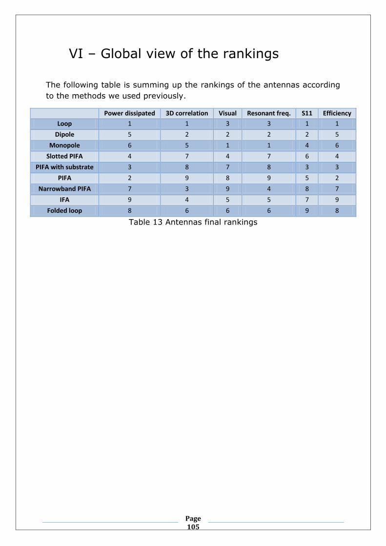
VI – Global view of the rankings
The following table is summing up the rankings of the antennas according
to the methods we used previously.
Power dissipated 3D correlation Visual Resonant freq. S11 Efficiency
Loop 1 1 3 3 1 1
Dipole 5 2 2 2 2 5
Monopole 6 5 1 1 4 6
Slotted PIFA 4 7 4 7 6 4
PIFA with substrate 3 8 7 8 3 3
PIFA 2 9 8 9 5 2
Narrowband PIFA 7 3 9 4 8 7
IFA 9 4 5 5 7 9
Folded loop 8 6 6 6 9 8
Table 13 Antennas final rankings
Page 106
Page 106
CONCLUSION
When we started this project, it was with the firm knowledge that we were
venturing into the unknown. There was little if not almost no theory
concerning the topic we chose and thin leads on the proper way to follow.
It was for us the occasion to see what pure research on uncharted
territories of science looked like, and for four month we dealt with
experimentation – some of it pertinent for what we looked for – but
unfortunately some of it of no use. All these experiments were, however,
a great leap of experience for all of us.
The main objective of this thesis was to find a brick to define properly the
human hand and a criterion for the robustness of antennas. Defining the
brick has come to be a success, allowing future research to simulate the
hand with an easier model to simulate the interactions of the antenna with
it. However, there was never one, but a great number of criterions for the
robustness. According to the main focus of the antenna (the S11, the
efficiency, the power dissipated…), the most robust antenna changed.
In the end, just like for the design of an antenna, there is mostly
simulation and experimentation that can really define the robustness of an
antenna, and not really a theoretical criterion.
Page 107
Page 107
References
[1] User’s Influence Mitigation for Small Terminal Antenna Systems,
Mauro Pelosi
[2] Computationnal Electrodynamics: The Finite Difference Time Domain
Method, Allen Taflove
[3] Antenna Theory Analysis and Design, Constantine A. Balanis
[4] http://mathbits.com/mathbits/tisection/statistics2/correlation.htm
[5] http://www.experiment-resources.com/pearson-product-moment-
correlation.html
[6] Les Antennes : Théories, conceptions et applications, Odile Picon
[7] http://www.antenna-theory.com/basics/impedance.php
[8] http://www.antenna-theory.com/antennas/smallLoop.php
[9] http://www.allenhollister.com/allen/files/scatteringparameters.pdf
[10] Lectures on microwaves Part 4- Smith Chart, Xavier Le Polozec, ECE
Paris 2010
[11] http://www.antenna-theory.com/tutorial/smith/chart.php#smithchart
[12] http://f5zv.pagesperso-
orange.fr/RADIO/RM/RM23/RM23p/RM23p01.html
[13] Interaction between mobile terminal antenna and user, Juho
Poutanen
[14] On the general energy absorption mechanism in the human tissue,
Outi Kivakäs, Tuukka Lehtiniemi, Pertti Vainikainen
[15] AAU3 User Manual