AALBORG UNIVERSITY

'

&

$

%

Monitoring Poisson time series usingmulti-process models

by

Malene C. Engebjerg, Søren Lundbye-Christensen,Birgitte B. Kjær and Henrik C. Schønheyder

R-2006-07 March 2006

Department of Mathematical SciencesAalborg University

Fredrik Bajers Vej 7G DK - 9220 Aalborg Øst DenmarkPhone: +45 96 35 80 80 Telefax: +45 98 15 81 29

URL: http://www.math.aau.dk eISSN 1399–2503 On-line version ISSN 1601–7811

Monitoring Poisson Time Series using Multi-ProcessModels

Malene C. Engebjerg

Department of Mathematical Sciences, Aalborg University, Aalborg, Denmark

Søren Lundbye-Christensen

Department of Mathematical Sciences, Aalborg University, Aalborg, Denmark

Birgitte B. Kjær

Department of Bacteriology, Mycoplogy and Parasitology, Statens Serum Institut, Copenhagen,Denmark

Henrik C. Schønheyder

Department of Clinical Microbiology, Aalborg Hospital, Aarhus University Hospital, Aalborg,Denmark

Abstract. Surveillance of infectious diseases based on routinely collected public health datais important for at least three reasons: The early detection of an epidemic may facilitate promptinterventions and the seasonal variations and long term trend may be of general epidemiolog-ical interest. Furthermore aspects of health resource management may also be addressed.In this paper we center on the detection of outbreaks of infectious diseases. This is achievedby a multi-process Poisson state space model taking autocorrelation and overdispersion intoaccount, which has been applied to a data set concerning Mycoplasma pneumoniae infections.

Keywords: Infectious disease, Outbreak, State space models, Surveillance, Warning system.

1. Introduction

Monitoring of routinely collected incidences of infectious diseases is of great importancein public health service. There may be at least three reasons for this. First of all earlydetection of the onset of an epidemic may provide the public health authorities with theinformation needed to make appropriate interventions. Secondly changes in seasonality orgeneral trend of a disease may be of epidemiological interest and finally aspects of resourcemanagement and quality control should not be underestimated. However, the number ofhealth-related information systems and the sheer amount of data available are beyond thelimits of manual surveillance and hence automated monitoring procedures are called for.

Farrington et al. (1996) describe an algorithm for the detection of outbreaks of infectiousdisease now being used at Statens Serum Institut, Denmark, in the monitoring of thegastointestinal pathogens Salmonella, Campylobacter, Yersinia, Shigella and E. coli, seeSSI (2005). Farrington et al. (1996) point out that timeliness, sensitivity and specificityare the main objectives of such an algorithm. This is accomplished through a log-linear

Address for correspondence: Malene C. Engebjerg, Department of Mathematical Sciences, Aal-borg University, Fredrik Bajers Vej 7G, DK-9220 Aalborg, DenmarkE-mail: maleneds@math.aau.dk

regression model, adjusted for overdispersion, seasonality, secular trends and past outbreaks.The model is then used to calculate a threshold-value above which any observed countsare flagged and further investigated. The threshold-value is calculated on the basis ofcorresponding weeks from previous years thereby incorporating the seasonal variation inthe data. However, if some of these weeks correspond to past outbreaks the threshold-valuewill be too high and hence the sensitivity declines. Consequently a weight function is definedgiving low weight to weeks with unusually high counts and in that way the threshold-valueis corrected for previous outbreaks.

A number of medical time series have been analyzed by Gordon and Smith (1990).The requirement was the detection of events of clinical or biological importance. This wasachieved using a multi-process Gaussian model, see Section 2.3, capable of handling missingvalues. In particular an application for monitoring renal transplants must be noted (a moredetailed description can be found in Smith and West (1983)).

Whittaker and Fruhwirth-Schnatter (1994) use a multi-process Gaussian model to detectthe possible time point at which bacteriological growth takes place in the monitoring offeedstuff. Whether one should stop sampling because bacteriological infection is highly likelyis determined by a decision rule which is defined in terms of the costs for false negativesand false positives.

Strat and Carrat (1999) illustrate how hidden Markov models may be used in monitoringsurveillance data. The approach actually mimics the multi-process models presented in thecurrent paper, Section 2.3 and 3, in that the observed series depends on an underlyingstate. Typically there are two states corresponding to a non-epidemic and an epidemicsituation. The states are assumed to follow a homogeneous Markov chain. There are,however, substantial differences between the two approaches. First of all Strat and Carrat(1999) adopt a non-Bayesian and a non-dynamic approach. The latter implies that the trendand seasonality are stationary quantities and hence do not vary over time. Furthermore themethod does not naturally incorporate on-line updating which is desirable when it comesto detection of outbreaks.

Cooper and Lipsitch (2004) go a step further and propose a structured hidden Markovmodel in the analysis of hospital infection data still in a non-Bayesian and non-dynamicsetup. The motive for this is that hospital infections are often only partially observed.This is overcome be letting the states correspond to the true number of patients who hasharbored the infection as opposed to the two (epidemic and non-epidemic states) proposedby Strat and Carrat (1999). The distribution of the observed series now depend on theunobserved state by assuming that the mean is proportional to the true number of infectedpatients. In this way autocorrelation and overdispersion in the observed series is takencare of. The term structured stems from the fact that a mechanistic understanding of thebiological and epidemiological nature of the data is incorporated into the model. This isachieved by defining the transition probabilities between the states in accordance with thestochastic susceptible-infectious-susceptible epidemic model. This has the clear advantagethat biological and epidemiological parameters may be estimated. This may prove to bevaluable in the understanding of the aetiology of an infection.

Finkenstadt and Grenfell (2000) propose a time series susceptible-infected-recoveredepidemic model for the analysis of measles data from England and Wales from 1944 to1964. In that way they also incorporate a mechanistic approach by defining a recursivestochastic relationship between the number of infected and susceptible individuals. Dueto under-reporting the number of infected individuals are only partially observed, whereasthe number of susceptible individuals are completely unknown. The model is fitted by

2

reconstructing the number of susceptible individuals using locally linear regression. Asopposed to Cooper and Lipsitch (2004) this approach is dynamic and better suited forpopulation modeling.

A much less complicated surveillance system based on weighted moving averages ispresented by Dessau and Steenberg (1993). It is intended for on-line surveillance andimplemented in a laboratory information system.

The objective of this paper has been to present a model which concisely incorporatesmany of the advantages of the above mentioned methods. This has been achieved by amulti-process Poisson model, where autocorrelation and overdispersion is handled via a la-tent process. The modeling of change-points is facilitated by the multi-process approach.Furthermore the approach is Bayesian, which allows for expert prior information to be di-rectly incorporated into the model. Finally a rigid description of the base activity is avoidedby letting the regression parameters vary randomly over time. The model is conceptuallysimple in nature and the setup is based on sequential updating equations which conformnicely to the requirement for on-line surveillance. In this paper, however, we have notadopted a mechanistic approach but only focused on surveillance and warning. We ap-ply this model to Danish nationwide laboratory data concerning Mycoplasma pneumoniaeinfections.

1.1. LayoutIn Section 2 we give a brief review of the basic state space models. In particular we will definethe dynamic linear model (DLM) (also denoted Gaussian state space model), where theobserved series is assumed to be conditionally Gaussian distributed given a latent process.We then proceed a step further by outlining the case, where the Gaussian assumptionis relaxed obtaining a dynamic generalized linear model (DGLM). Finally a multi-processGaussian model is presented, which extends the dynamic linear model by allowing any of afinite number of DLMs to describe the observation at any given time point.

Section 3 combines the dynamic generalized linear model with the multi-process Gaus-sian model to obtain a multi-process Poisson model, where one of the states is particularlydesigned to capture outliers. In this section we will give a detailed account of the updatingprocedures used in the multi-process Poisson model. In the implementation of the multi-process Poisson model some computational issues arose, which will be addressed in Section4. Section 5 contains an application to Mycoplasma pneumoniae infections and we end witha discussion in Section 6.

2. General State Space Models

Consider the time series

y1, y2, . . . , yt, . . .

observed at equally spaced time intervals, where yt is assumed to be a realization of Yt

for all t. The assumption of equispaced observations can easily be relaxed. Generally theobservations are thought to be autocorrelated as opposed to an independent and identi-cally distributed sample. In the present context the autocorrelation is partly due to thecommunicable nature of infectious diseases.

State space models provide a very general setup in which this autocorrelation is modeledvia a latent process, θt. The idea is that the observed series is considered conditional

3

independent given θt. Apart from the fact that a time series usually is autocorrelatedone often finds that a rigid description of the underlying mean is unsatisfactory. This isaccomplished in the state space setup by allowing the effect of the explanatory variables toevolve randomly over time.

An extension of the state space model as outlined above is the multi-process state spacemodel, which is achieved by combining a finite collection of state space models. Hence wedo not expect any single state space model to describe the data sufficiently throughout thestudy period. The multi-process model was first proposed by Harrison and Stevens (1971)and a more general account is given by Harrison and Stevens (1976).

2.1. Dynamic Linear ModelsThe model setup is as follows:

Yt = FTt θt + νt νt ∼ N [0, Vt] (1)

θt = Gtθt−1 + ωt ωt ∼ N [0, Wt] (2)

with prior information given by

(θ0 |D0) ∼ N [m0, C0]. (3)

Here Ft is a p×1 regression vector, θt is a p×1 parameter vector and Gt is a p×p evolutionmatrix. The error series {νt, ωt; t = 1, 2, . . .} is assumed to be mutually independent. Wenote that Vt, Wt, Ft, Gt, m0 and C0 are specified by the modeler.

Furthermore Dt denotes any historical information at time t relevant for the system in-cluding Vt, Wt, Ft, Gt, m0 and C0. Furthermore we will assume that any future informationset Dt will be closed to external information, i.e.

Dt = {yt, Dt−1} for t = 1, 2, . . . .

An account of the recursive updating scheme used for this univariate dynamic linearmodel can be found in West and Harrison (1999).

2.2. Dynamic Generalized Linear ModelsWe assume in the dynamic linear model that p(Yt |θt, Vt) is a Gaussian density. In thedynamic generalized linear model this density is replaced with a general density from theexponential family, i.e.

p(yt | ηt, Vt) = exp(V −1t (ytηt − a(ηt)))b(yt, Vt).

We then propose the following model:

g(µt) = λt = FTt θt

θt = Gtθt−1 + ωt ωt ∼ [0, Wt]

with prior information (θ0|D0) ∼ [m0, C0], where [·, ·] denotes a distribution which is onlypartially specified through the mean and variance. Again the error series {ωt; t = 1, 2, . . . }is assumed to be mutually independent.

Most often the canonical link function g will be used, that is to say the function gsatisfying g(µt) = ηt. In the Poisson case g(·) = log(·). See West and Harrison (1999) for atreatment of the dynamic generalized linear model.

4

2.3. Multi-Process Gaussian ModelsThe multi-process Gaussian models allow for sudden changes in pattern, not described bythe random variation in the latent process. This is accomplished by augmenting the dynamiclinear model with a discrete process, Mt indicating which one in a range of possible modelsapplies at a given time. This process could e.g. distinguish between an epidemic and anon-epidemic situation. The description of aberrant states is usually done by specifyinglarger evolutional or observational variances.

Furthermore we assume that model Mt(it) pertains at time t with probability π(it)irrespective of the past, i.e.

P(Mt |Mt−1, . . . , M1, Dt−1) = P(Mt |D0) = π(it).

This is also known as fixed model selection probabilities. In some applications a first orhigher order Markov model for Mt might be appropriate.

3. Multi-Process Poisson Models

In applications to count-data – e.g. the number of disease occurrences in a given timeperiod – the normal assumption will typically be inappropriate and therefore a multi-processPoisson model is presented in the current section. Here we will combine the methods givenin Section 2.2 and 2.3 to specify a multi-process model in the case where the observationsare assumed to be Poisson distributed. The combination of the dynamic generalized linearmodel and the multi-process Gaussian model is straightforward except for the specificationof the outlier model. This is due to the fact that the dispersion parameter in the Poissondistribution is 1. On the other hand it is essential in public health surveillance to be ableto distinguish an outlier from a permanent shift in the latent process. This stems from thefact that the accumulation of sporadic cases is immaterial in the detection of an epidemic.

In an unpublished research report West (1986) presents another approach to the multi-process model which applies much more generally in that the observations are merely as-sumed to follow an exponential family sampling distribution. On the other hand the outliermodel specified by West differs considerably from the outlier model offered in this paper.The main difference is that the sampling model is state independent in West (1986), whereaswe propose a state dependent sampling model specially designed for the Poisson case andin that way this is more reminiscent of the multi-process Gaussian model.

Yet another approach to the multi-process Poisson model has been made by Bolstad(1995). Here the modeling is restricted to the case, where the logarithm of the intensity isdescribed by a straight line and the states correspond to (1) steady state, (2) level changeand (3) outlier. In that way the handling of the different states is closely tied together withthe actual model proposed.

The model setup in this paper is as follows.For it = 1, 2, . . . , N (N being the number of different states) we define

Yt |µt, Mt = it ∼ Pois(µt∆it) (4)

log(µt) = ηt = FTt θt (5)

θt = Gtθt−1 + ωt, ωt |Mt = it ∼ [0, Wt(it)], (6)

with fixed model selection probabilities π. The error series {ωt; t = 1, 2, . . .} is assumedconditional independent given all model states.

5

����

����

����

����

����

����

����

����

����

����

����

����

yt−1 yt yt+1

Mt−1 Mt Mt+1

~ωt−1 ~ωt ~ωt+1

~θt−1~θt

~θt+1

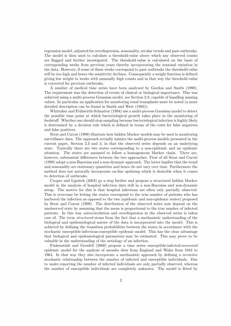
Figure 1. Directed Acyclic Graph (DAG) from which conditional independence relations may beidentified.

One may prove that the joint distribution as specified above admits a recursive factor-ization according to the graph shown in Figure 1. Any conditional independence relationsstated in the following can readily be identified from this graph, see Lauritzen (1996) orEdwards (2000) for an account on graphical models. The parameter ∆it

is the main ingre-dient in the outlier model. For any non-outlier state ∆it

= 1, a large outlier is specifiedby choosing ∆it

> 1 and similarly a small outlier by setting ∆it< 1. This implies that

the forecaster needs to define two or more ∆it-values if he wants to be able to predict both

small and large outliers. This may seem as a drawback. There is, however, at least tworeasons which justify this outlier model. The outlier model is transparent and the size of∆it

corresponds to the amount by which a potential outlier is expected to be above or belowthe mean value. The Poisson model is primarily necessary when the observed counts areexpected to be relatively small. Whenever this is the case small outliers will be indistin-guishable from the remaining observations and there will be no need for ∆it

-values less than1. In all other cases the multi-process Gaussian model will usually provide a satisfactoryapproximation.

The variances Wt(it) are once again used to specify the steady state model as well asany change model the forecaster finds appropriate. A sudden change in e.g. growth rate ismodeled by an appropriate elevation of the evolutional variance corresponding to the slopecomponent.

As in the multi-process Gaussian model the prior for θt is only partially specified throughits mean and variance. However, we will later force a conjugate prior upon µt given informa-tion on the last k + 1 models. This will basically superimpose distributional bindings uponall the above parameters although an exact distribution of these will be far too complicatedto take into account.

The updating scheme – also known as the multi-process Kalman filter – has been de-composed into 8 steps all of which will be described in the sequel.

3.1. Sequential Updating Equations

For notational convenience we will in the following abbreviate Mt = it with Mt, (Mt, . . . , Mt−j)with M t

t−j and similarly (it, . . . , it−j) with itt−j .

6

Input to the updating scheme at time tBeyond the regression vector Ft, the evolution matrix Gt, the covariance matrices {Wt(it)}

Nit=1

and the model selection probabilities {π(it)}Nit=1 we assume that

(θt−1 |Mt−1t−k , Dt−1) ∼

[

mt−1(it−1t−k), Ct−1(i

t−1t−k)

]

and that the joint probability p(M t−1t−k |Dt−1) is known. Note here that k denotes the lag

time.

InitializationIf t = 1 we let

(θ0 |M01−k, D0) ≡ (θ0 |M0, D0) ∼ [m0, C0]

and p(M01−k |D0) is left undefined.

The iterative updating scheme then proceeds as follows.

Step 1 [Conditional prior for θt and ηt]Using (5) and (6) the moments

(θt |Mtt−k, Dt−1) ∼ [at(i

t−1t−k), Rt(i

tt−k)],

(ηt |Mtt−k, Dt−1) ∼ [ft(i

t−1t−k), qt(i

tt−k)] (7)

and

Cov (ηt, θt |Mt(itt−k), Dt−1) = FT

t Rt(itt−k).

can easily be found.

Step 2 [Conjugate conditional prior for µt]To get a conjugate updating scheme we premise (µt |M

tt−k, Dt−1) to be Gamma distributed

with, say, form parameter rt(itt−k) and scale parameter st(i

tt−k). This implies that

p(ηt |Mtt−k, Dt−1) ∝ exp(rt(i

tt−k)ηt − st(i

tt−k) exp(ηt)).

One must now choose the parameters rt(itt−k) and st(i

tt−k) such that the prior moments for

ηt are as in (7). Making a first order Taylor expansion of µt(itt−k) around exp(ft(i

t−1t−k)) and

using the mean and variance of µt(itt−k) we get

exp(ft(it−1t−k)) ≃

rt(itt−k)

st(itt−k)and qt(i

tt−k) exp(2ft(i

t−1t−k)) =

rt(itt−k)

st(itt−k)2,

which lead us to choose rt(itt−k) and st(i

tt−k), for each combination of states itt−k, in the

following way

rt(itt−k) = (qt(i

tt−k))−1

st(itt−k) = (exp(ft(i

t−1t−k)) · qt(i

tt−k))−1.

7

Step 3 [Conditional predictive distribution for yt]The predictive distribution for yt is found by marginalization in the joint distribution for(yt, µt |M

tt−k, Dt−1):

p(yt |Mtt−k, Dt−1) =

∫

p(yt|µt, Mtt−k, Dt−1)p(µt |M

tt−k, Dt−1)dµt.

The former density on the right only depends on (µt, Mt) and is Poisson with parameterµt∆it

. Since the latter density is conjugate to the Poisson distribution the integrand is seento be proportional to a Γ(yt + rt(i

tt−k), ∆it

+ st(itt−k))-density and hence the normalization

constant can easily be found. Therefore the predictive density is

p(yt |Mtt−k, Dt−1) = ∆yt

it·

1

yt!·Γ(yt + rt(i

tt−k))

Γ(rt(itt−k))·

(st(itt−k))rt(i

tt−k)

(∆it+ st(itt−k))yt+rt(it

t−k).

Step 4 [Conjugate conditional posterior for µt]The conditional posterior for µt is given by (µt |M

tt−k, Dt) ∼ Γ(yt + rt(i

tt−k), ∆it

+st(itt−k))

and therefore the posterior moments for ηt are explicitly given in accordance with thisrelation although difficult to derive in closed form. However, Taylor expanding log(µt)around its posterior mean yields

(ηt |Mtt−k, Dt) ∼ [f∗t (itt−k), q∗t (itt−k)],

where

f∗t (itt−k) ≃ log( yt + rt(i

tt−k)

∆it+ st(itt−k)

)

and q∗t (itt−k) ≃ (yt + rt(itt−k))−1.

Step 5 [Conditional prior for (θt | ηt)]Recall from step 1 that

(

θt

ηt

∣

∣

∣

∣

M tt−k, Dt−1

)

∼

[(

at(it−1t−k)

ft(it−1t−k)

)

,

(

Rt(itt−k) Rt(i

tt−k)Ft

FTt Rt(i

tt−k) qt(i

tt−k)

)]

.

As this prior fails to be specified completely the moments for (θt | ηt, Mtt−k, Dt−1) are un-

known. However, using linear Bayes’ estimation, see West and Harrison (1999)[pp. 122],we may approximate the mean and variance by

(θt | ηt, Mtt−k, Dt−1) ∼ [a∗t (i

tt−k), R∗t (i

tt−k)],

where

a∗t (itt−k) ≃ at(i

t−1t−k) + Rt(i

tt−k)Ft(ηt − ft(i

t−1t−k))/qt(i

tt−k)

and

R∗t (itt−k) ≃ Rt(i

tt−k)−Rt(i

tt−k)FtF

Tt Rt(i

tt−k)/qt(i

tt−k).

Note that this corresponds to what we would have found had the above prior been Gaussian.

8

Step 6 [Posterior model probabilities for M tt−k]

For notational convenience we let

pt(itt−j) = p(M t

t−j |Dt), j = 1, 2, . . . , k.

To update the posterior probability pt(itt−k) note that

pt(itt−k) ∝ p(yt |M

tt−k, Dt−1)p(M t

t−k |Dt−1)

= p(yt |Mtt−k, Dt−1)p(Mt |M

t−1t−k , Dt−1)p(M t−1

t−k |Dt−1).

Since Mt is independent of the past the above reduces to

pt(itt−k) ∝ p(yt |M

tt−k, Dt−1)pt−1(i

t−1t−k)π(it). (8)

The first term on the right hand side was found in step 3 and the last term is specified bythe forecaster. At last the probability pt−1(i

t−1t−k) was given as input to the algorithm.

Step 7 [Posterior model probabilities for M tt−k+1]

At time t + 1 the updating scheme assumes the conditional probability pt(itt−k+1) to be

known which easily follows from step 6:

pt(itt−k+1) =

N∑

it−k=1

pt(itt−k).

Step 8 [Conditional posterior for θt]Finally the posterior mean and variance for θt must be provided for the updating at timet + 1. Suppose that (θt |M

tt−k+1, Dt) has a density. Then

p(θt |Mtt−k+1, Dt) =

N∑

it−k=1

p(θt |Mtt−k, Dt)

pt(itt−k)

pt(itt−k+1),

where the weights pt(itt−k)/pt(i

tt−k+1) were found in step 6 and 7. Inserting the linear Bayes’

estimate from step 5 yields

(θt |Mtt−k+1, Dt) ∼ [mt(i

tt−k+1), Ct(i

tt−k+1)],

where

mt(itt−k+1) =

N∑

it−k=1

pt(itt−k)

pt(itt−k+1)a∗t (i

tt−k)

and

Ct(itt−k+1) =

N∑

it−k=1

pt(itt−k)

pt(itt−k+1)

∫

(θt −mt(itt−k+1))

2p(θt |Mtt−k, Dt)dθt

=

N∑

it−k=1

pt(itt−k)

pt(itt−k+1)·(

R∗t (itt−k) + (a∗t (i

tt−k)−mt(i

tt−k+1))

2)

.

9

Here x2 = xxT . Since the distribution of (θt |Mtt−k+1, Dt) is only partially specified via

the first and second order moments there is no issue of collapsing densities here as opposedto the updating scheme for the multi-process Gaussian model.

3.2. Output at time tThe previous section presented the recursive updating equations used to run the multi-process Kalman filter. However, other outputs might be of interest in an application of themulti-process Poisson model some of which will be given below.

j-step back model probabilitiesThe j-step back model probabilities are

p(Mt−j |Dt) =

N∑

it−k=1

· · ·

N∑

it−j−1=1

N∑

it−j+1=1

· · ·

N∑

it=1

pt(itt−k)

for it−j = 1, 2, . . . , N and j = 0, 1, . . . , k.

Unconditional posterior for µt

Recall from step 4 that

(µt |Mtt−k, Dt) ∼ Γ(yt + rt(i

tt−k), ∆it

+ st(itt−k)).

Proceeding as above

E(µt |Dt) =

N∑

it=1

· · ·

N∑

it−k=1

pt(itt−k)

yt + rt(itt−k)

∆it+ st(itt−k)

= ht

and

Var (µt |Dt) =

N∑

it=1

· · ·

N∑

it−k=1

pt(itt−k)

(

yt + rt(itt−k)

(∆it+ st(itt−k))2

+( yt + rt(i

tt−k)

∆it+ st(itt−k)

− ht

)2)

.

Unconditional posterior for θt

Step 8 gave that

(θt |Mtt−k+1, Dt) ∼ [mt(i

tt−k+1), Ct(i

tt−k+1)]

and calculations analogous to those in step 8 yield that

(θt |Dt) ∼ [mt, Ct],

where

mt =

N∑

it−k+1=1

· · ·

N∑

it=1

pt(itt−k+1)mt(i

tt−k+1)

10

and

Ct =

N∑

it−k+1=1

· · ·

N∑

it=1

pt(itt−k+1) · (Ct(i

tt−k+1) + (mt(i

tt−k+1)−mt)

2).

3.3. Backward FilteringIn monitoring e.g. medical time-series the posterior model probabilities found in Section 3.1will often be an intrinsic part of the surveillance procedure. These probabilities should becompared with the corresponding filtered marginal distributions of (µt−j |Dt). In generalwe therefore seek the first and second order moments of (θt−l |Dt), where we will assumethat 1 ≤ l ≤ k. If we furthermore assume that t ≥ l + k no boundary value problemsoccur. The filtered marginal moments for (µt−l |Dt) may then be approximated by Taylorexpanding exp(FT

t−lθt−l), see Appendix A.

4. Computational Issues

The above updating scheme has been implemented in the statistical software package R,see R Development Core Team (2005). Here one has to make special attention as long ast ≤ k since in that case the dimension of some of the above computations are different fromthe one stated.

Furthermore numerical problems arose in step 3 and 8 both of which will be addressedin the current section.

Numerical problems in step 3Suppressing the indexes the likelihood function may be rewritten as

p(y | ·) =

(

s∆+s

)r

if y = 0

∆y(

∏y

i=1y+r−i

(y−(i−1))(∆+s)

)(

s∆+s

)r

if y > 0.

However s and r may be quite large which courses R to round off s/(∆ + s) to 1 such that(s/(∆+ s))r is set equal to 1 although it may be considerably smaller than 1. To overcomethis note that

( s

∆ + s

)r

=(

1 +∆

s

)

−r

=(

1 +∆exp(f)

r

)

−r

,

where we have used the relations between r, s, f and q given in step 2. The limit

limr→∞

(

1 +∆exp(f)

r

)

−r

= exp(−∆exp(f))

proves useful whenever r is large since the right hand side causes no numerically problemsin R.

We have computed the difference between (1 + x/r)−r and exp(−x) as a function ofr for x ∈ {0.1, 0.5, 1, 3, 5, 7} in R. Visual inspection revealed that the discrepancies for r

11

approximatively less than 104 was due to the poor approximation that exp(−x) providesfor (1 + x/r)−r. However, as r approaches 1012 the disagreement is caused by numeri-cal instability in R when computing (1 + x/r)−r . Therefore we have chosen to use theapproximation, whenever r > 107.

Numerical problems in step 8

In calculating the posterior mean and variance for θt division by pt(itt−k+1) is required.

Albeit, in theory, pt(itt−k+1) is strictly positive, R may round it off to 0 making the division

impossible. This will particularly be the case if the lag k is high and (it, . . . , it−k+1) allcorrespond to non-steady states. In that case we have used π(it−k) as weights in step 8instead of the correct pt(it−k | i

tt−k+1).

5. Application

Mycoplasma pneumoniae is a frequent cause of respiratory infections in both children andadults worldwide, see Baum (2005). The type of infection diagnosed most frequently ispneumonia with an estimated annual incidence of one per 1000 persons; the incidence ofnon-pneumonic respiratory infections may be 10-20 times as high. Mycoplasma pneumo-niae accounts for 1-8 percent of cases of pneumonia admitted to hospital in adulthood, seeBartlett and Mundy (1995), but far more cases are dealt with by general practitioners.Diagnostic tests include detection of specific antibodies and DNA-based methods such aspolymerase chain reaction (PCR). In Denmark, Statens Serum Institut has offered a cen-tralized diagnostic service for many years. This has revealed a distinctive picture of seasonalvariation with a peak during the winter half-year and epidemics every 3 to 5 years, see Lindet al. (1997). However, other epidemiological patterns may occur, see Baum (2005). Antibi-otics which normally are a first choice for patients with mild or moderate pneumonia maynot provide coverage for Mycoplasma pneumoniae, and therefore a reliable and timely alertof an increased incidence of Mycoplasma pneumoniae would allow physicians in primarycare as well as in hospitals to adjust empirical antibiotic therapy. The following data set(July 1994 to July 2005) represents samples of respiratory secretions submitted from all ofDenmark to Statens Serum Institut for examination by PCR, see Jensen et al. (1989).

Let Yt denote the total number of PCR-positive samples obtained at day t, t = 1, 2, . . . ,3132, where t = 1 corresponds to the 1st of January 1997. We then propose the followingmodel:

Yt |µt, Mt(it) ∼ Pois(µt∆it)

log(µt) = λt + γt

where the trend λt is described as a linear growth with random perturbations in level andslope:

λt = λt−1 + βt + δλt

βt = βt−1 + δβt.

The seasonal variation γt is a simple sine curve with period 365.25 and random perturbations

12

in amplitude,√

a2t + b2

t , and phase, − arccos(at/√

a2t + b2

t ):

γt = at sin(φt) + bt cos(φt)

at = at−1 + δat

bt = bt−1 + δbt.

Here φt = 2πt/365.25. Let

θTt = (λt, βt, at, bt).

Then the evolution equation can be written in matrix form as θt = Gθt−1 + ωt, where

G =

1 1 0 00 1 0 00 0 1 00 0 0 1

and ωt =

δλt + δβt

δβt

δat

δbt

and log(µt) = FTt θt with

FTt =

[

1 0 sin(φt) cos(φt)]

.

The period from the 1st of July 1994 to the 31th of December 1996 was used as input tothe analogous generalized linear model in order to obtain a bet for the prior mean m0. Theprior variance C0 is defined as a diagonal matrix with the square root of the diagonals beingequal to

σprior(λ0) = 3 · 10−5 σprior(β0) = 4 · 10−4

σprior(a0) = 3 · 10−5 σprior(b0) = 3 · 10−5.

We defined the following three model states: 1) steady state, 2) level and slope change and3) outlier state, where the second is meant to represent an epidemic situation, in which theevolution shows erratic behaviour in level as well as in slope. Let σj(X) correspond to thestandard deviation of the random variable X when model j applies. The modelling of thethree states was achieved by defining

σ1(δλt) = σ1(δβt) = 1 · 10−7

σ1(δat) = σ1(δbt) = 1 · 10−6

and

σ2(δλt) = σ2(δβt) = 0.5.

These values were all found empirically. Then

Wt(j) =

σ2j (δλt) + σ2

j (δβt) σ2j (δβt) 0 0

σ2j (δβt) σ2

j (δβt) 0 0

0 0 σ2j (δat) 0

0 0 0 σ2j (δbt)

.

13

Finally we let

(∆1, ∆2, ∆3) = (1, 1, 5)

corresponding to an outlier having a five-fold intensity compared with the current level.Furthermore

(π(1), π(2), π(3)) = (99.85%, 0.1%, 0.05%)

implying a prior belief of approximately 3 level and slope changes and 1− 2 outliers in thetime period analyzed.

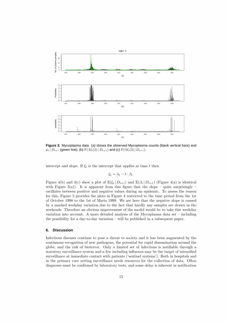
Figure 2 and 3 show (a) the observed Mycoplasma counts (black vertical bars) andµt |Dt+lag (green line), (b) P(Mt(2) |Dt+lag) and (c) P(Mt(3) |Dt+lag) for lag = 0, 1, re-spectively. Clearly there has been a large epidemic in the winter 1998/1999 and a lessprominent one in the winter 2004/2005. It is evident from Figure 2 that the multi-process

Lag = 0

(a)

No.

of p

ositi

ve s

ampl

es

1997 1998 1999 2000 2001 2002 2003 2004 2005

020

6010

0

(b)

Pro

babi

lity

1997 1998 1999 2000 2001 2002 2003 2004 2005

0.0

0.2

0.4

0.6

0.8

1.0

(c)

prob

abili

ty

1997 1998 1999 2000 2001 2002 2003 2004 2005

0.0

0.2

0.4

0.6

0.8

1.0

Figure 2. Mycoplasma data. (a) shows the observed Mycoplasma counts (black vertical bars) andµt | Dt (green line), (b) P(Mt(2) | Dt) and (c) P(Mt(3) | Dt).

model initially interprets the large counts observed in 1998/1999 and 2004/2005 as corre-sponding to either level and slope changes or outliers. On the other hand there seems to beno false positives in the very early prediction of an epidemic. Figure 3 reveals that lookingjust one day back in time greatly improves the discrimination between the epidemic andthe outlier state and it is obvious that the model is able to recognize departures from thenon-epidemic situation.

From Figure 3 it appears as if (µt |Dt+1) alternates between high and low values duringan epidemic. This might be accessed by exploring the one-step back distribution for the

14

Lag = 1

(a)

No.

of p

ositi

ve s

ampl

es

1997 1998 1999 2000 2001 2002 2003 2004 2005

020

6010

0

(b)

Pro

babi

lity

1997 1998 1999 2000 2001 2002 2003 2004 2005

0.0

0.2

0.4

0.6

0.8

1.0

(c)

prob

abili

ty

1997 1998 1999 2000 2001 2002 2003 2004 2005

0.0

0.2

0.4

0.6

0.8

1.0

Figure 3. Mycoplasma data. (a) shows the observed Mycoplasma counts (black vertical bars) andµt | Dt+1 (green line), (b) P(Mt(2) | Dt+1) and (c) P(Mt(3) | Dt+1).

intercept and slope. If ξt is the intercept that applies at time t then

ξt = λt − t · βt.

Figure 4(b) and 4(c) show a plot of E(ξt |Dt+1) and E(βt |Dt+1) (Figure 4(a) is identicalwith Figure 3(a)). It is apparent from this figure that the slope – quite surprisingly –oscillates between positive and negative values during an epidemic. To assess the reasonfor this, Figure 5 provides the plots in Figure 4 restricted to the time period from the 1stof October 1998 to the 1st of Marts 1999. We see here that the negative slope is causedby a marked weekday variation due to the fact that hardly any samples are drawn in theweekends. Therefore an obvious improvement of the model would be to take this weekdayvariation into account. A more detailed analysis of the Mycoplasma data set – includingthe possibility for a day-to-day variation – will be published in a subsequent paper.

6. Discussion

Infectious diseases continue to pose a threat to society and it has been augmented by thecontinuous recognition of new pathogens, the potential for rapid dissemination around theglobe, and the risk of bioterror. Only a limited set of infections is notifiable through astatutory surveillance system and a few including influenza may be the target of intensifiedsurveillance at immediate contact with patients (’sentinel systems’). Both in hospitals andin the primary care setting surveillance needs resources for the collection of data. Oftendiagnoses must be confirmed by laboratory tests, and some delay is inherent in notification

15

(a)

No.

of p

ositi

ve s

ampl

es

1997 1998 1999 2000 2001 2002 2003 2004 2005

020

6010

0

(b)

Inte

rcep

t

1997 1998 1999 2000 2001 2002 2003 2004 2005

010

0030

00

(c)

Slo

pe

1997 1998 1999 2000 2001 2002 2003 2004 2005

−1.

5−

0.5

0.5

Figure 4. Mycoplasma data. (a) shows the observed Mycoplasma counts (black vertical bars) andµt | Dt+1 (green line), (b) the evolution of the intercept E(ξt | Dt+1) and (c) the slope E(βt | Dt+1).

procedures. Dependent on the scope of the surveillance system data are aggregated atregional, national or international level. Although numbers of observations may be large forsome categories of infections others remain rare as exemplified by the nearly 2000 differenttypes of Salmonella. Legionella infections is another example of a rare event even withdata from the entire Europe, see Joseph (2004). For infections not being a target of formalsurveillance systems useful information may still be available from health administrativesystems such as hospital discharge registries and laboratory information systems. Healthservices automatically cumulate such data in dedicated databases with little delay and theypertain to the population served. Inherently, the numbers of observations will often besmall.

Thus there are basically two applications of the proposed warning system: First ofall it may support existing statutory surveillance systems especially in situations with rareoccurrences. Secondly it may be embedded locally in the health administrative system wheredata are already available but where automated surveillance usually is not implemented.Thus the Poisson assumption of the presented model encompasses the handling of both ofthese surveillance situations. This implies a unified model approach in all situations, thePoisson assumption being crucial especially for surveillance of relatively rare events.

Furthermore the model is highly modular in the sense that separate models are for-mulated for the change-point component, the evolutional component and the observationalcomponent. It deserves notice that there is a conceptual difference between the change-pointcomponent and the evolutional component: In the change-point component the expectedfrequency of aberrant incidents is specified whereas the evolutional component describes the

16

(a)

No.

of p

ositi

ve s

ampl

es

okt−1998 nov−1998 dec−1998 jan−1999 feb−1999 mar−1999

020

6010

0

(b)

Inte

rcep

t

okt−1998 nov−1998 dec−1998 jan−1999 feb−1999 mar−1999

010

0030

00

(c)

Slo

pe

okt−1998 nov−1998 dec−1998 jan−1999 feb−1999 mar−1999

−1.

5−

0.5

0.5

Figure 5. Mycoplasma data from the 1st of October 1998 to the 1st of Marts 1999. (a) shows theobserved Mycoplasma counts (black vertical bars) and µt | Dt+1 (green line), (b) the evolution of theintercept E(ξt | Dt+1) and (c) the slope E(βt | Dt+1).

nature of the steady state behavior and the relevant aberrations. The evolutional compo-nent is itself modular as e.g. the seasonal variation, trend and other effects are modeledseparately. This adds transparency and flexibility into the model specification. Moreoverextensions and generalizations are easily adapted in this modular structure.

In the application we have focused on the posterior model probabilities, i.e. the proba-bility of the occurrence of a recent change-point in the time series. Output on a probabilityscale has several advantages: Foremost it will be familiar to most of the expert users ofthe surveillance system. For specific applications the model may be integrated in a decisionsupport system provided that dependable estimates of the associated costs of false positivesand negatives can be obtained.

There is a versatility of other possible outputs from the proposed model. The posteriormoments of the evolutional component contain information valuable for quality control, re-source management purposes or epidemiological research. In laboratory information systemsthe former will primarily manifest itself in the surveillance of specific specimens, where un-expected changes in the base activity may stem from laboratory inconsistencies, see Dessauand Steenberg (1993). Examples of output relevant for resource management could be thecontemporary growth rate or the expected number of counts within a specified time frame.Gradual changes in the pattern of seasonal variation, e.g. the peak-to-trough ratio or thetime for peak may, on the other hand, be of general epidemiological interest, and can bevaluable output for observational studies.

An issue yet to be solved is the calibration of such models. So far the applicability

17

of the model necessitate the disposal of learning data and the calibration is more or lessobtained by trial-and-error. There is hence a need for the development of efficient parameterestimation methods.

Acknowledgements

We thank Anders Koch and Thomas Hjuler, Department of Epidemiology Research, StatensSerum Institut, Denmark for construction and advice on use of the mycoplasma database.

A. Backward Filtering

Input to the updating scheme at time tSuppose that at time t the updating procedure described in Section 3.1 has been run andassume that

(θt−l+1 |Mtt−k, Dt) ∼ [m

(l−1)t (itt−k), C

(l−1)t (itt−k)] (9)

is known and that 1 ≤ l ≤ k.

l-step back filteringThe idea is to find the moments of (θt−l |θt−l+1, M

tt−k, Dt) and then use (9) to find

m(l)t (itt−k) and C

(l)t (itt−k).

Now

p(θt−l |θt−l+1, Mtt−k, Dt) ∝ p(y |θt−l+1, θt−l, M

tt−k, Dt−l)p(θt−l |θt−l+1, M

tt−k, Dt−l),

where y = (yt, . . . , yt−l+1). Knowing (θt−l+1, Mtt−k, Dt−l) it follows that y is independent

of θt−l and hence the above reduces to

p(y |θt−l+1, Mtt−k, Dt−l)p(θt−l |θt−l+1, M

tt−k, Dt−l)

∝ p(θt−l |θt−l+1, Mtt−k, Dt−l)

∝ p(θt−l+1 |θt−l, Mtt−k, Dt−l)p(θt−l |M

tt−k, Dt−l).

Since k ≥ l the model at time t− l+1 appears in the first conditioning and hence the aboveis equal with

p(θt−l+1 |θt−l, Mt−l+1)p(θt−l |Mt−lt−k, Dt−l),

where we have used that p(θt−l |Mtt−k, Dt−l) does not depend on the future.

The evolution equation in (6) implies that

(θt−l+1 |θt−l, Mt−l+1) ∼ [Gt−l+1θt−l, Wt−l+1(it−l+1)].

Appropriately weighting the moments of (θt−l |Mt−lt−l−k+1, Dt−l) (found in step 8) with

pt−l(it−k−1t−l−k+1 | i

t−lt−k) (step 7) yields

(θt−l |Mt−lt−kDt−l) ∼ [bt−l(i

t−lt−k), Bt−l(i

t−lt−k)].

18

The fact that the above two distributions are only partially specified via their first andsecond order moments implies that the mean and variance of

(θt−l |θt−l+1, Mtt−k, Dt)

are not well-defined. The mean and variance are therefore set equal to the linear Bayesestimates. Suppressing the subscripts these are given by

E(θt−l |θt−l+1, Mtt−k, Dt) = bt−l + Bt−lG

Tt−l+1U

−1(θt−l+1 −Gt−l+1bt−l), (10)

where

U = U(it−l+1t−k ) = Gt−l+1Bt−l(i

t−lt−k)GT

t−l+1 + Wt−l+1(it−l+1)

and

Var (θt−l |θt−l+1, Mtt−k, Dt) = Bt−l −Bt−lG

Tt−l+1U

−1Gt−l+1Bt−l. (11)

Applying the above together with (9) and the relations E(X) = E(E(X |Y )) and Var (X) =E(Var (X |Y )) + Var (E(X |Y )) yields

(θt−l |Mtt−k, Dt) ∼ [m

(l)t (itt−k), C

(l)t (itt−k)],

where

m(l)t (itt−k) = bt−l(i

t−lt−k) + Bt−l(i

t−lt−k)GT

t−l+1U−1(m

(l−1)t (itt−k)−Gt−l+1bt−l(i

t−lt−k))

and

C(l)t (itt−k) = Bt−l(i

t−lt−k)−Bt−l(i

t−lt−k)GT

t−l+1U−1Gt−l+1Bt−l(i

t−lt−k)+

Bt−l(it−lt−k)GT

t−l+1U−1C

(l−1)t (itt−k)U−1Gt−l+1Bt−l(i

t−lt−k).

This finally implies that

E(θt−l |Dt) =

N∑

it=1

pt(itt−k)m

(l)t (itt−k) = v

(l)t

and

Var (θt−l |Dt) =N∑

it=1

pt(itt−k) ·

[

C(l)t (itt−k) +

(

m(l)t (itt−k)− v

(l)t

)2]= V

(l)t .

Therefore

E(ηt−l |Dt) = FTt−lv

(l)t = f

(l)t and

Var (ηt−l |Dt) = FTt−lV

(l)t Ft−l = q

(l)t .

Taylor expansion to the first order of µt−l = exp(ηt−l) around f(l)t yields

E(µt−l |Dt) ≃ exp(f(l)t ) and

Var (µt−l |Dt) =≃ exp(2f(l)t )q

(l)t .

19

Initialization

To initialize the above updating scheme we need the mean and variance of

(θt |Mtt−k, Dt)

both of which were given in step 1 in Section 3.1.

References

Bartlett, J. and L. M. Mundy (1995, December). Community-acquired pneumonia. NewEngland Journal of Medicine 333 (24), 1618–1624.

Baum, S. G. (2005). Mycoplasma pneumoniae and atypical pneumonia. In G. Mandell,J. Bennett, and D. Raphael (Eds.), Mandell, Douglas, and Bennett’s Principles andPractice of Infectious Diseases, pp. 2271–2280. Elsevier Inc. Philadelphia PA.

Bolstad, W. M. (1995, March). The Multiprocess Dynamic Poisson Model. Journal of theAmerican Statistical Association 90 (429), 227–232.

Cooper, B. and M. Lipsitch (2004). The analysis of hospital infection data using hiddenMarkov models. Biostatistics 5 (2), 223–237.

Dessau, R. B. and P. Steenberg (1993, April). Computerized Surveillance in Clinical Mi-crobiology with Time Series Analysis. Journal of Clinical Microbiology 31 (4), 857–860.

Edwards, D. (2000). Introduction to Graphical Modelling. Springer-Verlag New York, Inc.ISBN 0-387-95054-0.

Farrington, C., N. Andrews, A. Beale, and M. Catchpole (1996). A Statistical Algorithm forthe Early Detection of Outbreaks of Infectious Disease. Journal of the Royal StatisticalSociety. Series A 159 (3), 547–563.

Finkenstadt, B. F. and B. T. Grenfell (2000). Time series modelling of childhood diseases:a dynamical systems approach. Applied Statistics 49 (2), 187–205.

Gordon, K. and A. Smith (1990, June). Modelling and Monitoring Biomedical Times Series.Journal of the American Statistical Association 85 (410), 328–337.

Harrison, P. and C. Stevens (1971, December). A Bayesian Approach to Short-term Fore-casting. Operational Research Quarterly 22 (4), 341–362.

Harrison, P. and C. Stevens (1976). Bayesian Forecasting. Journal of the Royal StatisticalSociety. Series B 38 (3), 205–247.

Jensen, J. S., J. Søndergard-Andersen, S. A. Uldum, and K. Lind (1989, November). Detec-tion of Mycoplasma pneumoniae in simulated clinical samples by polymerase chain reac-tion. Brief report. Acta Pathologica, Microbiologica et Immunologica Scandinavica 97 (11),1046–1048.

Joseph, C. A. (2004). Legionnaires’ disease in Europe 2000-2002. Epidemiology and Infec-tion 132 (3), 417–424.

20

Lauritzen, S. L. (1996). Graphical Models. Oxford University Press Inc., New York. ISBN0-19-852219-3.

Lind, K., M. W. Benzon, J. S. Jensen, and W. A. J. Clyde (1997, July). A seroepidemio-logical study of Mycoplasma pneumoniae infections in Denmark over the 50-year period1946-1995. European Journal of Epidemiology 13 (5), 581–586.

R Development Core Team (2005). R: A language and environment for statistical com-puting. Vienna, Austria: R Foundation for Statistical Computing. ISBN 3-900051-07-0,http://www.R-project.org.

Smith, A. and M. West (1983, December). Monitoring Renal Transplants: An Applicationof the Multiprocess Kalman Filter. Biometrics 39 (4), 867–878.

SSI (2005). Beregning af udbrudsstatus. Statens Serum Institut, Denmark.http://www.ssi.dk/graphics/html/udbrudmonitor/siderne/Hovedindex.htm, (accessed2005-12-19).

Strat, Y. L. and F. Carrat (1999). Monitoring epidemiologic surveillance data using hiddenMarkov models. Statistics in Medicine 18 (24), 3463–3478.

West, M. (1986). Non-normal multi-process models. Technical Report Research Report 81,Department of Statistics, University of Warwick.

West, M. and J. Harrison (1999). Bayesian Forecasting and Dynamic Models. Springer.ISBN 0-387-94725-6.

Whittaker, J. and S. Fruhwirth-Schnatter (1994). A Dynamic Changepoint Model for De-tecting the Onset of Growth in Bacteriological Infections. Applied Statistics 43 (4), 625–640.

21