AALTO UNIVERSITY

SCHOOL OF ELECTRICAL ENGINEERING

Department of Electrical Engineering

Bishal Silwal

Computation of eddy currents in a solid rotor induction machine

with 2-D and 3-D FEM

Thesis supervisor:

Professor Antero Arkkio

Thesis instructor:

Docent Anouar Belahcen

ii

STRACT

AALTO UNIVERSITY

SCHOOL OF ELECTRICAL ENGINEERING Abstract of the Master’s Thesis

Author: Bishal Silwal

Name of the topic: Computation of eddy currents in a solid rotor induction machine with

2-D and 3-D FEM

Date: 24.04.2012 Language: English Number of pages: ix+62

Department of Electrical Engineering

Professorship: Electromechanics Code: S-17

Supervisor: Professor Antero Arkkio

Instructor: Docent Anouar Belahcen

Abstract

Although a two-dimensional numerical analysis of an electrical machine provides an

approximately accurate solution of the electromagnetic field in the machine, a three-

dimensional study is needed to understand the actual phenomena. But due to the large

problem size and the complex geometries, the three dimensional model requires a huge

amount of degrees of freedoms (DoFs) to be solved, which is not possible with a limited

computing resources. Therefore, a coupled 2D-3D model can be the best alternative to

solve such type of problems.

In this thesis, a 2-D finite element analysis is performed on a solid rotor induction motor

by an in-house software FCSMEK. The eddy current in the solid steel rotor was

computed. A 3-D model for the same machine was built and solved in COMSOL

Multiphysics™. To reduce the computation time of the 3-D model, the solution of the 2-

D model was used as the source to the 3-D model where the stator current density is used

as a transferred variable. The eddy currents are computed and the results from both 2-D

and 3-D simulations are compared. Other quantities of interest such as the torque of the

machine computed with the 2-D and 3-D models are also computed and compared.

Keywords: Electrical Machines, Finite Element Method (FEM), Eddy Currents, Coupled

Models

iii

ACKNOWLEDGEMENT

My master’s thesis is a part of a research project that is funded by the Academy of

Finland. Firstly, I am indebted to my instructor Dr. Anouar Belahcen for his

support, encouragement, ideas and advice ranging from the minute technical

details to the overall research process. His guidance helped me to learn a lot from

this project. A sincere thanks goes to my supervisor Prof. Antero Arkkio for his

support and motivation through-out the research process. A share of thanks goes

to the Head of the Department of Electrical Engineering Prof. Asko Niemenmaa

for creating a good working and research environment.

I would also like to express my gratitude to Mr. Ari Havisto for helping me by

managing all the technical resources required for this thesis. I would also like to

thank other members of the Electromechanic Research group such as Javiar

Martinez, Paavo Rasilo, Van Khang Huynh, Mikko Heino and Ansi Sinvervo,

with whom I have had many productive discussions. I heartily thank Deepak

Singh and Tuomas Janhunen for their support and ideas that helped me a lot

during the simulations.

I would also like to thank all the members of the Nepalese community here at

Aalto University for always making this place a lively place to live in. Special

thanks to Subash Khanal for helping me during the tough days.

Last but not least, I express my sincere gratitude to my parents Mr. Niranjan

Silwal and Mrs. Janaki Silwal, my sisters Sanju, Ranju and Bijita and other

relatives for their care, support and love, and also to my girlfriend Neha for her

love, support and for understanding me and also for being very inquisitive about

what I was doing.

Espoo, April 24, 2012

Bishal Silwal

iv

TABLE OF CONTENTS

ABSTRACT ....................................................................................................................... ii

ACKNOWLEDGEMENT ................................................................................................ iii

TABLE OF CONTENTS .................................................................................................. iv

LIST OF FIGURES .......................................................................................................... vi

LIST OF SYMBOLS AND ABBERVIATION ............................................................... viii

CHAPTER 1: INTRODUCTION ....................................................................................10

1.1 Background ................................................................................................................10

1.2 Objectives ..................................................................................................................13

1.3 Outline of the Thesis .................................................................................................14

CHAPTER 2: LITERATURE AND METHODOLOGY ...............................................15

2.1 Solid Rotor Induction Motor .........................................................................................15

2.2 Maxwell’s Equation in brief ........................................................................................19

2.3 Finite Element Method (FEM) ......................................................................................21

2.4 Eddy Current Formulations ......................................................................................23

2.5 Time-Stepping Analysis ...........................................................................................27

2.6 Methodology ..............................................................................................................28

CHAPTER 3: FEM MODELS AND SIMULATIONS ...................................................30

3.1 Machine Parameters ....................................................................................................30

3.2 2-D Finite Element Simulation in FCSMEK .................................................................32

3.3 Results from FCSMEK .............................................................................................35

3.4 3-D Physical Model ......................................................................................................41

3.5 Data Transfer ...............................................................................................................44

3.6 Simulation in COMSOL Multiphysics™ ......................................................................45

3.6.1 2-D Model ............................................................................................................45

3.6.2 3-D Model ............................................................................................................51

CHAPTER 4: RESULTS AND DISCUSSIONS .............................................................56

4.1 Results from 2-D Simulation ........................................................................................56

4.2 Results from 3-D Simulation ........................................................................................59

CHAPTER 5: CONCLUSION .........................................................................................63

v

REFRENCES .....................................................................................................................66

APPENDIX A ....................................................................................................................68

APPENDIX B ....................................................................................................................71

vi

LIST OF FIGURES

Figure 2.1: Smooth solid steel rotor . ........................................................................ 16

Figure 2.2: Solid Rotor Constructions ....................................................................... 18

Figure 2.3: First order linear triangular element ........................................................ 22

Figure 2.4: Triangular elements on a circular geometry . ........................................... 22

Figure 2.5: Eddy current problem. ............................................................................ 23

Figure 3.1: 2-D cross-section of the machine under study ......................................... 30

Figure 3.2: BH Curve of the stator core material. ...................................................... 32

Figure 3.3: BH Curve of the stator core material. ..................................................... 33

Figure 3.4: Finite Element Simulation steps used in FCSMEK for 2D study. ............ 34

Figure 3.5 Finite element mesh in the symmetric cross-section using FCSMEK. ....... 35

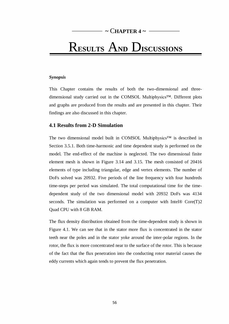
Figure 3.6: Computed magnetic flux density distribution in the cross-section of the

machine .................................................................................................................. 37

Figure 3.7: Computed magnetic flux density distribution in the computed region along

with the motion of the rotor shown ........................................................................... 37

Figure 3.8: Three-phase current in the stator winding computed by the TSA ............. 39

Figure 3.9: Time variation of Torque computed with the TSA. ................................. 39

Figure 3.10: Eddy current distribution in the rotor surface. ....................................... 40

Figure 3.11: Shape and dimension parameters of the stator slot ................................. 42

Figure 3.12: Rotor slit .............................................................................................. 43

Figure 3.13: 2-D cross-section of the machine build in SolidWorks™....................... 43

Figure 3.14: 3-D geometrical model ......................................................................... 44

Figure 3.15: Part of the two dimensional mesh used in the 2D simulation with the

commercial software COMSOL Multiphysics™ ....................................................... 49

Figure 3.16: A closer view to the mesh in the air gap ................................................ 49

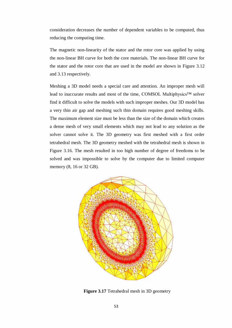
Figure 3.17: Tetrahedral mesh in 3D geometry ......................................................... 53

Figure 3.18: Prism mesh created by sweeping the triangular mesh ............................ 54

Figure 4.1: Magnetic flux density distribution and the flux lines as computed with

TSA in the COMSOL Multiphysics™ ...................................................................... 57

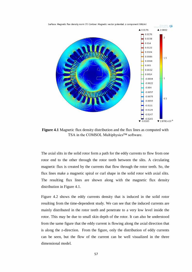
Figure 4.2: Eddy current density distribution. ........................................................... 58

vii

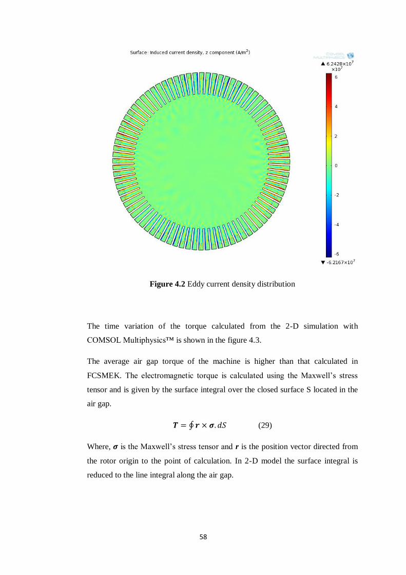
Figure 4.3: Torque variation resulting from 2-D simulation in COMSOL

Multiphysics™ ......................................................................................................... 59

Figure 4.4: Three dimensional flux density distribution computed with the 3D

simulation in COMSOL Multiphysics™ ................................................................... 60

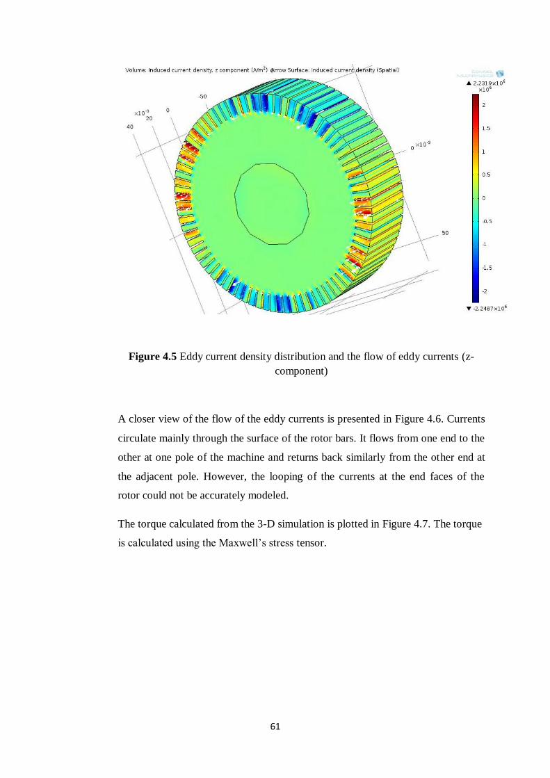
Figure 4.5: Eddy current density distribution and flow of eddy currents. ................... 61

Figure 4.6: Computed z-component of the eddy currents. ......................................... 62

Figure 4.7: Torque variation resulting from 3-D simulation in COMSOL

Multiphysics™ ......................................................................................................... 62

viii

LIST OF SYMBOLS AND ABBERVIATION

δ

ε

µ

ρ

σ

φ

ψ

ωr

ωs

Ω

Lamination Thickness

Permittivity

Magnetic Permeability

Electric Charge Density

Conductivity

Reduced Electric Scalar Potential

Reduced Magnetic Scalar Potential

Angular Speed of Rotor

Angular Speed of Stator

Magnetic Scalar Potential

A Magnetic Vector Potential

B

f

E

H

I

J

n

ns

Pe

Ph

R

s

T

V

V

BEM

CAD

Magnetic Flux Density

Frequency

Electric Field Strength

Magnetic Field Strength

Current

Current Density

Rotor Speed

Synchronous Speed

Eddy Current Loss

Hysteresis Loss

Resistance

slip

Electric Vector Potential

Voltage

Electric Scalar Potential

Boundary Element Method

Computer Aided Design

ix

FEM

FDM

PDE

rpm

rps

THA

TSA

Finite Element Method

Finite Difference Method

Partial Differential Equation

Revolution per Minute

Revolution per Second

Time-Harmonic Analysis

Time-Stepping Analysis

10

~ CHAPTER 1 ~

INTRODUCTION

1.1 Background

Machines have always made life simpler, directly or indirectly. The development

of an electrical machine began when Michael Faraday first demonstrated the

conversion of electrical energy to mechanical energy through electromagnetic

field in 1821. Since then numerous researches were done all around the globe to

develop and apply electrical machines to make things easier, and today we stand

where various ac and dc machines have been developed for a wide range of

applications.

For the performance analysis of any machine, one important parameter to be

considered is the machine loss. This consideration has significances like

determining the efficiency of the machine which in turn influences the operating

cost, determining the heating of machine which gives the machine rating without

the deterioration of insulation, and for accounting the voltage drops or current

component associated with the cause of the losses. Losses in electrical machines

can be categorized according to the causes or phenomena that produce them. For

instance, the Copper Loss or Ohmic Loss is the I2R loss caused when a current I

flows through the winding (copper in most cases) having a resistance R. The

losses due to the friction in the brushes and bearing and windage losses are

altogether considered to be the mechanical losses. The friction and windage losses

can be measured by determining the unloaded and unexcited machine input at

proper speed but generally they are lumped with core loss and determined at the

same time. The Stray Load Loss is one kind of losses in electrical machines that

arises from the non-uniform distribution of current in winding and the additional

core losses produced in the iron due to the distortion of the magnetic flux caused

by the load current. One major loss that highly affects the performance of the

machine is the Core Loss. As the name depicts, it is the loss that occurs in the core

of the machine, generally the iron part. In simple words, it is caused due to the

11

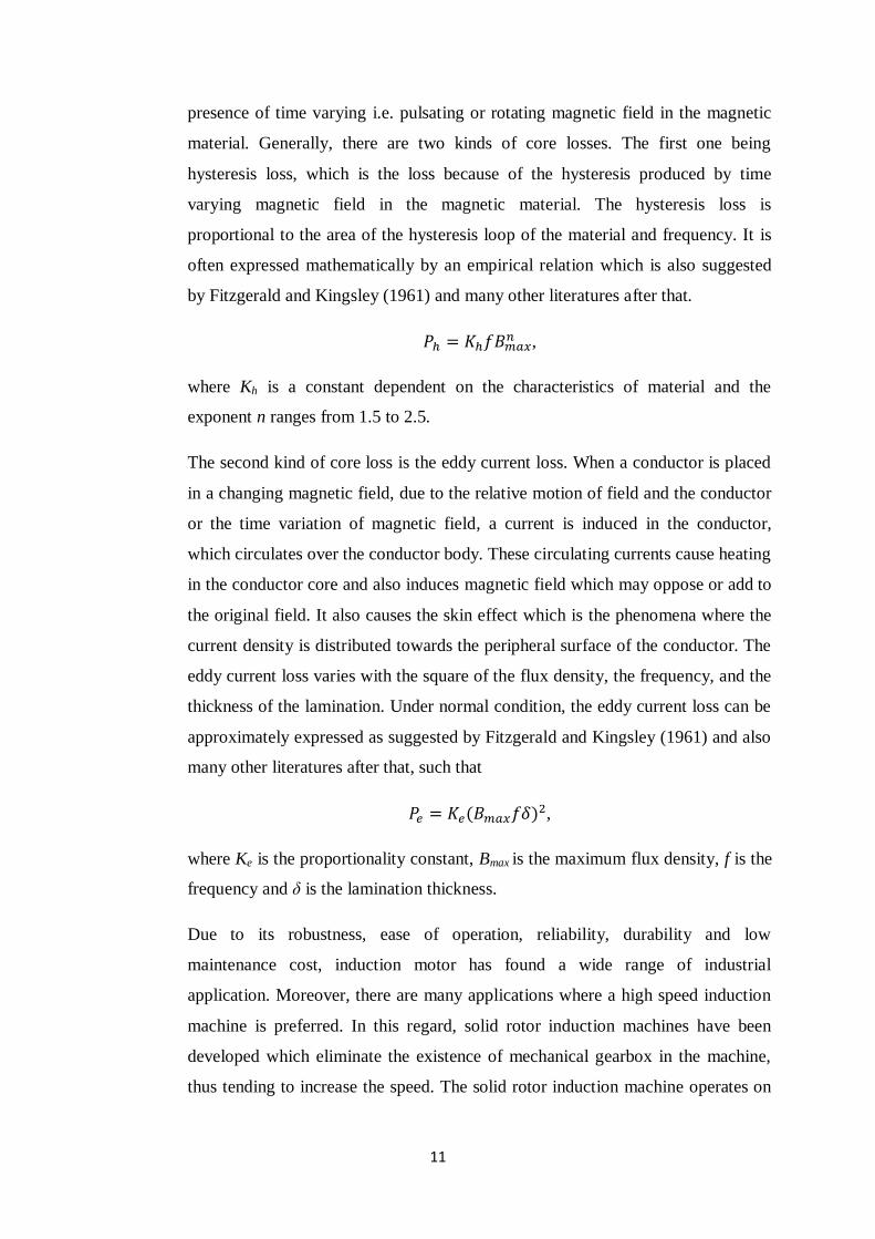
presence of time varying i.e. pulsating or rotating magnetic field in the magnetic

material. Generally, there are two kinds of core losses. The first one being

hysteresis loss, which is the loss because of the hysteresis produced by time

varying magnetic field in the magnetic material. The hysteresis loss is

proportional to the area of the hysteresis loop of the material and frequency. It is

often expressed mathematically by an empirical relation which is also suggested

by Fitzgerald and Kingsley (1961) and many other literatures after that.

,

where Kh is a constant dependent on the characteristics of material and the

exponent n ranges from 1.5 to 2.5.

The second kind of core loss is the eddy current loss. When a conductor is placed

in a changing magnetic field, due to the relative motion of field and the conductor

or the time variation of magnetic field, a current is induced in the conductor,

which circulates over the conductor body. These circulating currents cause heating

in the conductor core and also induces magnetic field which may oppose or add to

the original field. It also causes the skin effect which is the phenomena where the

current density is distributed towards the peripheral surface of the conductor. The

eddy current loss varies with the square of the flux density, the frequency, and the

thickness of the lamination. Under normal condition, the eddy current loss can be

approximately expressed as suggested by Fitzgerald and Kingsley (1961) and also

many other literatures after that, such that

,

where Ke is the proportionality constant, Bmax is the maximum flux density, f is the

frequency and δ is the lamination thickness.

Due to its robustness, ease of operation, reliability, durability and low

maintenance cost, induction motor has found a wide range of industrial

application. Moreover, there are many applications where a high speed induction

machine is preferred. In this regard, solid rotor induction machines have been

developed which eliminate the existence of mechanical gearbox in the machine,

thus tending to increase the speed. The solid rotor induction machine operates on

12

the same principle as that of conventional induction machines, but the physical

construction is different. Solid rotor is made up of a solid ferromagnetic body, for

example steel, and does not have any windings. The strong mechanical strength of

the solid rotor and its simple construction are also the prime reason of the use of

solid rotor machines in high speed applications. But, its lower efficiency and

power density play a vital role to degrade the machines performance where the

induced eddy currents in the ferromagnetic rotor body add more into it. In recent

years, research has been focused on the improvement of the efficiency of the high-

speed solid rotor machine. According to Huppunen (2004) it has been found that a

perfect sinusoidal flux density distribution on the rotor surface produces the

lowest possible losses in the solid rotor high speed machines and therefore flux

density distribution must be taken into important consideration in case of such

machines. The fact that the smooth solid rotor runs at quite a low per-unit slip

indicates that the efficiency of the machine can possibly be increased by reducing

the stator and rotor losses as well as the harmonic content of the air-gap flux.

The accuracy and precision of the study of any electrical machine highly depends

on what dimensional study we perform. So far both two dimensional and three

dimensional analyses of machines are in existence. The two dimensional analysis

is regarded to be simple and having low computational time because of relatively

lower number of unknown variables to be solved. However for understanding of

the exact phenomena, a three dimensional study of the machine is considered

which is relatively complex with respect to the two dimensional computation. If

we consider the numerical model or numerical analysis of the machine, the three

dimensional computation of the solution by taking into account the coupled

equations of different variables has not been reasonably possible. This is due to

the large amount of unknown variables it has to solve. This problem is expected to

be solved by a coupled two dimensional and three dimensional model. It can be

expected that this kind of coupled model is not only relatively fast to solve

because of the reduced number of unknowns but also gives an accurate result

within given computational resources. One example of such coupling can be the

coupling between the 2D model of the stator and a 3D finite element model of the

rotor of an induction machine, where the eddy currents induced in the rotor has to

be investigated as explained by Dziwniel et al. (1999).

13

This thesis is about the analysis of similar coupled two dimensional and three

dimensional model of a solid steel rotor high speed machine. The research work is

based on the coupling between the 2D model of the stator of the solid steel rotor

high speed machine with the 3D model of its rotor and is focused on the

computation of eddy currents in the rotor. The eddy currents will be computed

from the 2D simulation, and the same field solution result from the 2D analysis

will be used as a source to the 3D model of the rotor. The solution from the 2D

and 3D simulations will be compared. This will not only help to analyze the eddy

current loss distribution in the rotor surface but also assist to predict the

performance of machine under given load condition.

1.2 Objectives

This project deals with the study of the solid steel rotor high speed machine, the

study being based on the coupling between the 2D models of the stator of the

machine with the 3D model of its rotor to accurately investigate eddy currents in

the solid rotor parts without a need for a 3D model of the stator. The primary

objectives of the project can be listed as follows:

i. To study about different magneto-dynamic models in electromechanics and

various eddy current formulations in different dimension; literature review.

ii. To compute two dimensional field solution of the machine in an in-house

software.

iii. To construct a 3D model of the machine to be used for computation in a

commercial software.

iv. To use the two dimensional solution from the in-house software as the source to

the 3D model of the rotor in the commercial software and compute it.

v. To compare the eddy currents computed from both 2D and 3D simulations

vi. To write a Master’s Thesis based on all the computations, solutions and

comparison made.

14

1.3 Outline of the Thesis

The background behind the thesis and the objectives of the project are discussed

in Chapter 1. Chapter 2 highlights the finite element method and different

numerical formulations used for the solution of eddy current problems. The step

wise simulation process in the in-house software and its results are presented in

Chapter 3. This chapter also presents the details about the design of the 3D model

of the machine and also the simulations made in the commercial software. The

results of the 3D simulation are also presented in the same chapter. Chapter 4

compares and draws conclusions from the simulation results and also presents

possible potential areas of future research.

15

~ CHAPTER 2 ~

LITERATURE AND METHODOLOGY

Synopsis

This chapter deals with the brief introduction of different methods used for the

solution of boundary value problems in electromagnetics, with special

consideration to the numerical method using finite elements. A short introduction

of a solid rotor induction motor is presented at the start. Different magnetic vector

potential formulations used for the solution of eddy current problems are also

discussed in this chapter. It also provides brief introduction to the methodology

used in the project for solution of eddy current problems using finite element

methods.

2.1 Solid rotor induction motor

Electrical machines work on the principle of energy conversion process through

the electromagnetic field. From robotics to heavy load cranes, electrical machines

have always played a vital role. There are various types of machine developed so

far, which are categorized mainly with respect to their principle of operation and

then their applications. Induction machines are one kind of electrical machines

which are widely used in industrial drives and operate on the principle of

electromagnetic induction. When the stator winding is energized with a supply, it

creates a rotating magnetic field which then induces current in the rotor conductor.

This current in turn interacts with the rotating magnetic field thus causing the

rotation.

Solid rotor induction machine are special kind of induction machine in which the

rotor is a solid body made of low-conductivity ferromagnetic alloy. It has the

similar topology with the conventional induction machine with an exception in the

rotor construction which may be smooth solid rotor as discussed by Brunelli et al.

16

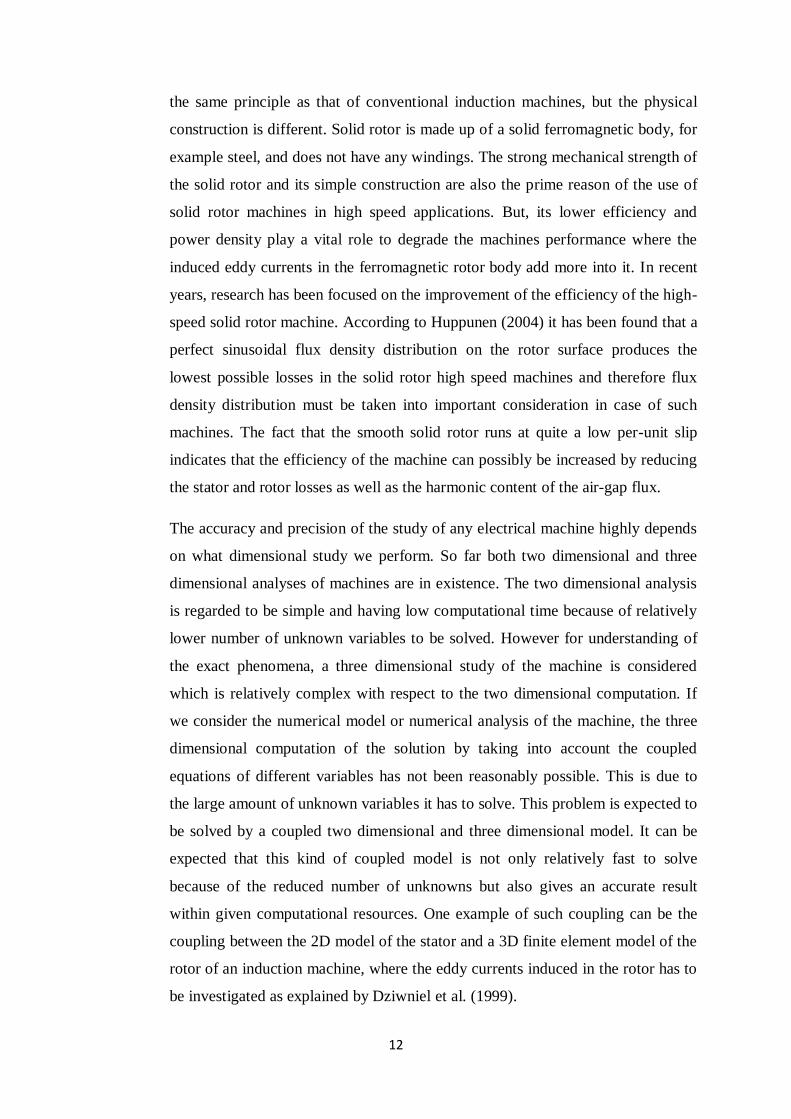
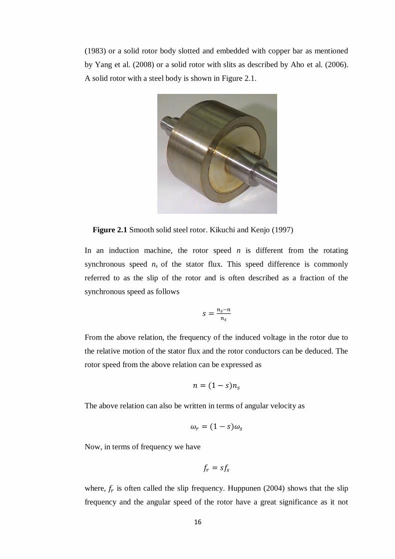
(1983) or a solid rotor body slotted and embedded with copper bar as mentioned

by Yang et al. (2008) or a solid rotor with slits as described by Aho et al. (2006).

A solid rotor with a steel body is shown in Figure 2.1.

Figure 2.1 Smooth solid steel rotor. Kikuchi and Kenjo (1997)

In an induction machine, the rotor speed n is different from the rotating

synchronous speed ns of the stator flux. This speed difference is commonly

referred to as the slip of the rotor and is often described as a fraction of the

synchronous speed as follows

From the above relation, the frequency of the induced voltage in the rotor due to

the relative motion of the stator flux and the rotor conductors can be deduced. The

rotor speed from the above relation can be expressed as

The above relation can also be written in terms of angular velocity as

Now, in terms of frequency we have

where, is often called the slip frequency. Huppunen (2004) shows that the slip

frequency and the angular speed of the rotor have a great significance as it not

17

only plays an important role in determining the penetration of magnetic flux in the

rotor but act as a factor to determine the torque produced by the rotor.

The solid rotor shown in Figure 2.1 is a smooth solid rotor with a steel body.

However, all solid rotors may not have a smooth body, as stated earlier. Ho et al.

(2010), in their research have shown that the existence of axial slits in the solid

rotor can cause the magnetic flux in the rotor to penetrate relatively deeper into

the rotor and the analysis shows that having slits in the solid rotor will increase

the torque of the machine by about 3.46 times than that of a rotor without slits.

Welding a well-conducting non-magnetic material at the end faces of the rotor and

equipping the solid rotor with a squirrel cage are two other possible ways to

enhance the performance of the solid rotor, while sometimes the smooth solid-

steel rotor may also be coated by a well conducting material for e.g. copper which

have been shown by Huppunen (2004) in his Doctoral Thesis. Different schematic

constructions of the solid rotor are shown in Figure 2.2.

Ho et al. (2010) also lists the advantages of the solid rotor induction machine as

follows:

Simplicity in its construction

Low production cost and easy manufacturing

High robustness against mechanical stress

High thermal reliability

High mechanical balance, stable

These merits are also supported by Gieras and Saari (2010) in their research paper

and they also showed that these merits make solid rotor machine superior in

applications that require high rotor strength, high critical speeds and good

balancing properties.

18

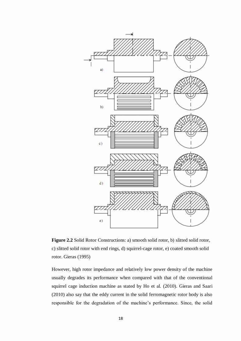
Figure 2.2 Solid Rotor Constructions: a) smooth solid rotor, b) slitted solid rotor,

c) slitted solid rotor with end rings, d) squirrel-cage rotor, e) coated smooth solid

rotor. Gieras (1995)

However, high rotor impedance and relatively low power density of the machine

usually degrades its performance when compared with that of the conventional

squirrel cage induction machine as stated by Ho et al. (2010). Gieras and Saari

(2010) also say that the eddy current in the solid ferromagnetic rotor body is also

responsible for the degradation of the machine’s performance. Since, the solid

19

rotor is made up of a conducting material, with lower conductivity though, it sets

a pathway for the magnetic flux as well as the induced eddy currents. This eddy

current induced in the solid rotor tends to increase the losses, which may in turn

lead to an increase of the temperature, thus degrading the performance of the

machine. Therefore, eddy current loss and its distribution in the case of solid rotor

machine has been a significant field of study with the aim to predict the machine

performance and to find the ways to improve it.

2.2 Maxwell’s Equations

Jackson (1999) in his book explains that the electric field and magnetic field can

be considered to be almost independent when dealing with steady-state problems,

but this independent nature no longer lasts when we consider a time-dependent

problem. Time varying magnetic fields give rise to the electric fields and vice

versa, which brings up a combined electrical and magnetic field term called

electromagnetic. There are a set of equations that describe the fundamentals of

electromagnetic fields and space and time relationship between electricity and

magnetism. These equations are known as Maxwell’s Equation. The differential

form of Maxwell’s Equation can be expressed as follows

(1)

(2)

(3)

(4)

where,

is the electric field strength

is the magnetic field strength

is the electric flux density

is the magnetic flux density

20

is the electric current density

is the electric charge density

The Maxwell Equations expressed above are simply the equations that describe

four different laws in the field of electricity and magnetism. These different laws

are more illustratively described when the Maxwell Equations are expressed in the

integral form. The equations (1)-(4) can be expressed in the integral form by the

use of the Gauss Theorem and the Stokes Theorem. Using Gauss Theorem on a

volume V and its boundary surface S, the integral form of (1) and (2) can be

obtained and expressed as

∮ ∮ (5)

∮ (6)

Similarly using Stokes’s Theorem and taking the integration over an open surface

S and its boundary path s, we get the integral form for the equations (3) and (4)

which can be expressed as

∮ ∮

(7)

∮ ∮ (

) (8)

Equations (5) and (6) describe the Gauss Law for Electricity and Magnetism

respectively. Equation (5) relates the electric flux density with the total charge

enclosed. It illustrates that the outflow of the electric flux density vector D over

the closed surface S equals to the free electric charge enclosed within the surface.

Similarly, equation (6) illustrates that the outflow of the magnetic flux density

vector B vanishes. The Faraday’s law of electromagnetic induction is described by

the equation (7). It illustrates how the time varying magnetic field creates an

electric field. Equation (8) generalizes the Ampere’s circuital law with Maxwell’s

addition of displacement current

. This equation is generally referred to as the

Ampere’s law with Maxwell’s correction.

The variables in the equations above are related with each other by a set of

constitutive relations that describes the different properties of the material and the

21

medium in which the material is placed. These constitutive relations can be

expressed as

(9)

(10)

(11)

where, is the permittivity, is the permeability and is the conductivity of the

material or medium in which the material is placed.

2.3 Finite Element Method (FEM)

Luomi (1993) presents his idea that electrical machines and other electromechanic

devices operate on the principle of energy conversion through the electromagnetic

field which makes their analysis to be done based on the solution of the field or on

its approximation. Development of traditional calculation methods have been

existed since long time, however, the recent development of computers and other

numerical methods have made it quite convenient to deal with more complicated

problems and moreover by solving the field equation directly. Finite Difference

Methods (FDM), Boundary Element Method (BEM) and Finite Element Method

(FEM) are some of the numerical methods used for solving the boundary value

problems where a continuous problem is discretized and then its differential

equation is solved by using a computer.

The main idea of Finite Element Analysis is to divide a large and complex

problem area into small and simple problem areas. The small problem area is

defined as an element. Then a solution is approximated in each small element

using a function, generally a polynomial. This process of dividing a geometric

model into small finite elements is called meshing. Figure 2.3 shows a first order

finite element and Figure 2.4 shows the division of a circular geometry into small

finite triangular elements.

22

Figure 2.3 First order triangular element; (xi,yi) is the node coordinate and ui is

the value of potential at node i.

Figure 2.4 Triangular elements on a circular geometry

After creating a mesh, we define the sources and the boundary values of the

problem. In each element, the solution (or potential) is approximated by using a

polynomial which will give the matrix representation of each element.

Approximation of the solution in each element by a polynomial will lead to an

expression for the solution as

∑ (12)

23

Where, Ni(x,y) is called the global shape function and is non-zero only in those

elements to which node i belongs to and n is the total number of nodes in the

problem region.

Combination of all elemental matrices will lead to the global system matrix. Then

we apply all the necessary boundary conditions and solve the resulting equations

to get the result.

Kanerva (2001) presents Finite Element Analysis as a powerful tool for the

analysis of magnetic fields in electrical machines and the electrical state of

different components of machine can also be derived based on that solution.

However, for proper analysis, both the magnetic field equation and the circuit

equation should be used in conjunction with each other, i.e. they must be coupled.

2.4 Eddy Current Formulations

In any electromechanical device accounting the time variation of magnetic field,

the variation of magnetic field with time will induce an electric field which in turn

will cause a current to flow in the conducting medium of the device. This current

is called eddy current. The induced eddy currents again tend to affect the magnetic

field. This is the reason why we need to solve both electric and magnetic field

equations together to solve the eddy current problems.

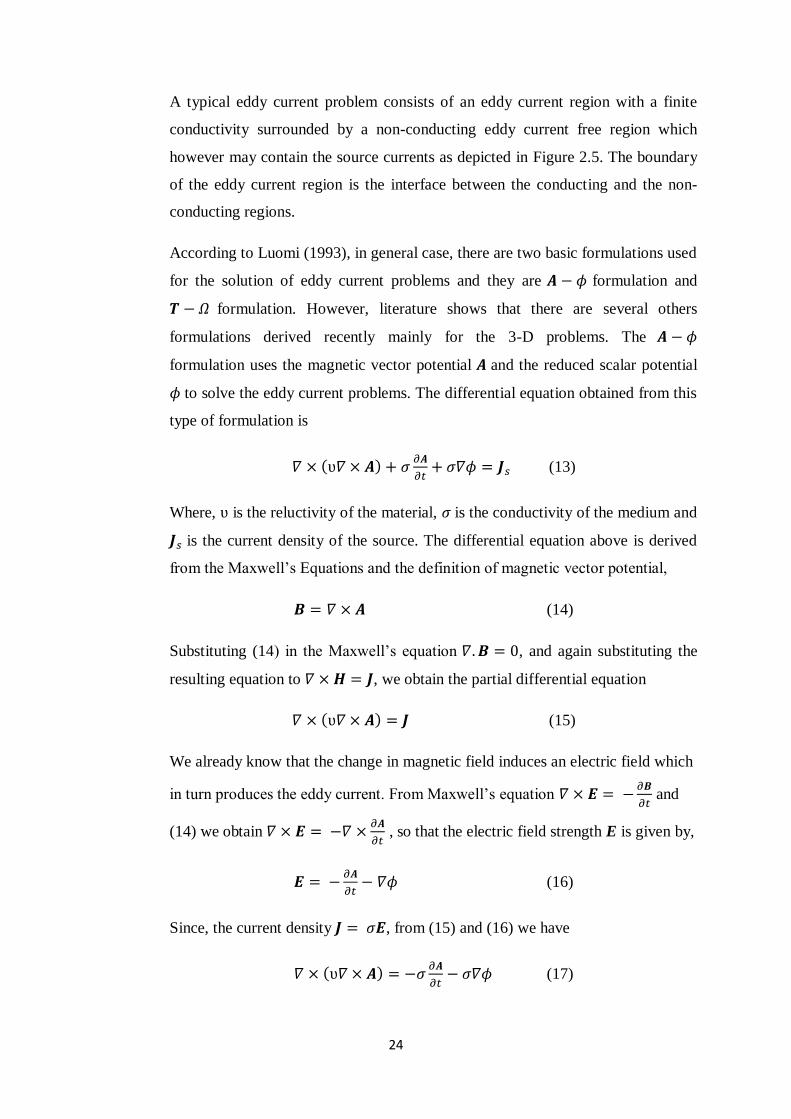
Figure 2.5 Eddy current problem

24

A typical eddy current problem consists of an eddy current region with a finite

conductivity surrounded by a non-conducting eddy current free region which

however may contain the source currents as depicted in Figure 2.5. The boundary

of the eddy current region is the interface between the conducting and the non-

conducting regions.

According to Luomi (1993), in general case, there are two basic formulations used

for the solution of eddy current problems and they are formulation and

formulation. However, literature shows that there are several others

formulations derived recently mainly for the 3-D problems. The

formulation uses the magnetic vector potential and the reduced scalar potential

to solve the eddy current problems. The differential equation obtained from this

type of formulation is

(13)

Where, is the reluctivity of the material, is the conductivity of the medium and

is the current density of the source. The differential equation above is derived

from the Maxwell’s Equations and the definition of magnetic vector potential,

(14)

Substituting (14) in the Maxwell’s equation , and again substituting the

resulting equation to , we obtain the partial differential equation

(15)

We already know that the change in magnetic field induces an electric field which

in turn produces the eddy current. From Maxwell’s equation

and

(14) we obtain

, so that the electric field strength E is given by,

(16)

Since, the current density , from (15) and (16) we have

(17)

25

The current density corresponding to (17) is the eddy current density as it is

produced by the electric field which is induced by the change in the magnetic

field, so (17) is valid for eddy current regions. But, the current density

corresponding to (15) is the source current density that is the current density in the

source coils and windings. So, both equations (15) and (17) are combined to give

a single equation which corresponds to the whole problem region which is

expressed as given in (13).

The divergence of the eddy current density vanishes, which gives us another

equation

(

) (18)

The tangential component for the electric field E and the normal component of

is continuous at the interface between the eddy current region and

non-eddy current region.

The electric vector potential and the magnetic scalar potential are used to

derive the formulation, where is defined such that . Also, the

magnetic field strength is defined as . From this definition of

magnetic field strength and Maxwell’s equation , we find that the curl

of the electric vector potential is equal to the current density, that is .

Now, the electric field E can be written as

and the magnetic flux

density B can also be written as . Substituting the

expression of E and B in Maxwell’s equation

, we obtain

(

)

[ ] (19)

Substituting the expression for in Maxwell’s equation , we obtain

another equation

(20)

In formulation, the tangential component of the magnetic field strength

must be continuous which makes the electric vector potential continuous at the

26

interface. Also the normal component of is continuous at the

interface.

In two dimensional eddy current problems, the magnetic vector potential, the

electric field strength and the current density are all z-directed and the field is

calculated in the xy-plane. The gradient is also z-directed and moreover the

assumption that there is no existence of potential differences due to the electric

charge (since the conductivity is assumed to be constant in the conducting region)

makes equal to zero. Thus the partial differential equation for the computation

of 2-D eddy current problems becomes

(21)

Now, this PDE is discretized to get a system of ordinary differential equation,

which is then solved by various methods like Euler Methods, Runge-Kutta

Method, Crank-Nicholson Method, Gear Method, Newton Method etc.

The three dimensional computation of eddy current fields has been the subject of

extensive research for the international community of numerical analysts. Their

dedicated to work on the investigation of electromagnetic field from early 80’s

which can be well understood by the number of scientific contributions in this

field seen at that time, for instance in Biro and Preis (1989). Various formulations

have been developed, generally based on the formulation or

formulations. formulation, formulation,

formulation are some examples of the formulations using magnetic vector

potential, reduced electric scalar potential and electric scalar potential. However,

the solution of large systems of equations leads to increased number of unknowns

which cause unreasonably high computation time and cost and 3-D calculations of

eddy current become very difficult which is also explained by Muller and

Knoblauch (1985) in their research. Various researches have been carried out to

overcome these difficulties.

27

In 3-D eddy current problems, both the electric and the magnetic field must be

described in the conductors while in the regions which are free from eddy

currents, only magnetic field needs be accounted for as presented by Biro and

Preis (1990). Biro and Preis (1990) also suggests that different sets of potentials

may be used in conducting and eddy current free regions but it may cause

problems while interfacing them on the conductor surface. Many formulations for

3-D eddy current problems have been developed in order to solve this problem.

formulation is obtained when the potentials in conductors are

coupled with outside the conductors. Similarly when the potentials in the

conductors are coupled with the in the eddy current-free regions,

formulation is obtained. Balchin and Davidson (1983) found out that advantages

of using the magnetic scalar potential in the non-conducting domain and

suggested that the use of in the non-conductor region instead of in the

formulation, the problem of having large number of unknowns

in the eddy current-free regions can be minimized and this gave the

formulation. Though formulation overcomes the difficulties of the

formulation, it is still unable to treat multiply connected conductors

which is also explained by Biro and Preis (1990). The problem of multiply

connected conductors can be possibly addressed through the method suggested by

Leonard and Rodger (1988) by using instead of in the non-conducting holes

of the conductors in the multiply connected conductors, which gives the

formulation.

2.5 Time-Stepping Analysis

The finite element analysis of an electrical machine, when only the sinusoidal

supply is considered is regarded as Time-Harmonic Analysis (THA). The

computational time in THA is quite short. But it does not consider some higher

harmonics and also the motion of the rotor is not accounted for. Therefore, Time-

Stepping Analysis (TSA) method is used in order to consider both the motion of

the rotor and the harmonics related to it. In this case, the circuit equations are also

solved together with the field equations. To consider the motion of the rotor, the

28

elements in the air gap are modified at each time step during the discretization of

the field equation as presented by Davat, Ren and Lajoie-Mazenc (1985). This

method of modeling the movement of the rotor in a machine model has also been

used and discussed by Arkkio (1990).

The partial differential equation (21) can be discretized to get a system of ordinary

differential equations, which can be then solved by different methods like Euler

Methods, Runge-Kutta Method, Crank-Nicolson Method, Gear Method, Newton

Method etc. However, a generalized first-order finite difference procedure can be

used to get a solution by time stepping. If, at time step tk-1, the nodal value is ak-1

then at time step tk, the nodal value ak is given by

[

|

|

]

where, Δt is the length of the time step; β is a weighting parameter between 0 and

1, the most popular values used for β being 0 for Direct Euler Method, 0.5 for

Crank-Nicolson (trapezoidal) method and 1for backward Euler method. These

values of β for the discretization process have also been used by Islam and Arkkio

(2008).

2.5 Methodology

This project mainly deals with the investigation of the solution of problems

related to the coupled field in electrical machine with different dimensions. The

investigation of a coupled 2D-3D model of solid rotor of a high speed induction

machine is the main agenda of the project where eddy current computation and

analysis is the primary interest.

After studying relevant literatures and gathering information and knowledge about

the background and literatures related to the project, the initial work was started

which consisted of computing the magnetic vector potential or magnetic flux

density in a two-dimensional model of the machine. For this purpose, an in-house

2D finite element software FSCMEK was used. A three-phase, 50 Hz, 380 V, star

connected, 7.5 kW solid rotor induction machine was considered. The rotor of the

29

machine is made up of a steel body with slits. The 2D model of the machine was

simulated. The solution obtained from this computation was to be used as a source

for the 3D model of the rotor. Since the in-house software FCSMEK was limited

to the 2D modeling only, the 3D modeling and computations were done using

commercial finite element software called COMSOL Multiphysics™. The 3D

CAD-model of the machine was constructed in SolidWorks™ and then imported

to the COMSOL Multiphysics™. The parameters of the model used for 3D

simulation were the same as these used in FCSMEK. After having obtained the

solution from 2-D simulation, the resulting nodal values of magnetic vector

potential were tried to use as a source in the 3-D model. Matlab was used for data

transfer between FCSMEK and COMSOL Multiphysics™. However, the task of

transferring the nodal values of the magnetic vector potential was very tedious.

So, an alternative way was chosen, that is using the current density in the stator

slots computed from FCSMEK as a source in the slots of the model in the 3-D

model. The 3D model was then simulated and then the eddy current loss was

calculated. This eddy current loss was compared with the one obtained from the

2D solution in FCSMEK.

30

~ CHAPTER 3 ~

FEM MODELS AND SIMULATIONS

Synopsis

This chapter deals with the details of all the simulations carried out during the

study. Firstly, it describes the 2D simulations performed in the in-house software

and its results. The construction of both the physical and the finite element 3-D

model is also well described in this chapter. All the definitions and assumptions

made for the modeling are included here.

3.1 Machine Parameters

This study deals with the investigation of eddy current loss calculation in solid

steel rotor of an induction machine. Both 2-D and 3-D models of the machine are

taken into account and computation based on finite element method is carried out.

The machine under study is considered to be a three phase, 50 Hz, 380 V, star

connected, 7.5 kW solid steel rotor induction machine. The cross-section of the

machine under study is shown in Figure 3.1 and the machine parameters are listed

in Table 3.1.

Figure 3.1 2-D cross-section of the machine under study

31

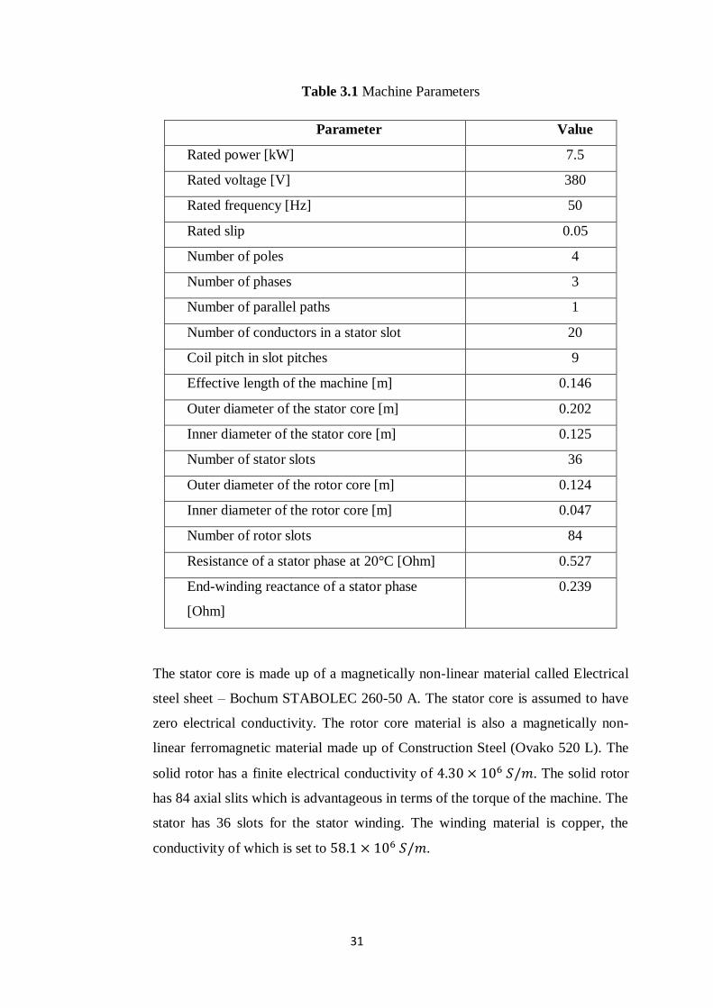
Table 3.1 Machine Parameters

Parameter Value

Rated power [kW] 7.5

Rated voltage [V] 380

Rated frequency [Hz] 50

Rated slip 0.05

Number of poles 4

Number of phases 3

Number of parallel paths 1

Number of conductors in a stator slot 20

Coil pitch in slot pitches 9

Effective length of the machine [m] 0.146

Outer diameter of the stator core [m] 0.202

Inner diameter of the stator core [m] 0.125

Number of stator slots 36

Outer diameter of the rotor core [m] 0.124

Inner diameter of the rotor core [m] 0.047

Number of rotor slots 84

Resistance of a stator phase at 20°C [Ohm] 0.527

End-winding reactance of a stator phase

[Ohm]

0.239

The stator core is made up of a magnetically non-linear material called Electrical

steel sheet – Bochum STABOLEC 260-50 A. The stator core is assumed to have

zero electrical conductivity. The rotor core material is also a magnetically non-

linear ferromagnetic material made up of Construction Steel (Ovako 520 L). The

solid rotor has a finite electrical conductivity of . The solid rotor

has 84 axial slits which is advantageous in terms of the torque of the machine. The

stator has 36 slots for the stator winding. The winding material is copper, the

conductivity of which is set to .

32

3.2 2D Finite Element Simulation in FCSMEK

The initial step of the investigation was to perform a finite element analysis of the

2 dimensional model of the given machine. For this purpose, the in-house finite

element software FCSMEK was used. The software has a collection of programs

and routines designed for the finite element analysis of synchronous and

asynchronous radial flux machines.

The machine parameters mentioned in Table 3.1 among others were given as an

input file to the software. The software creates geometry from the parameters in

the input file. The equations to be solved are also defined in the program of the

software. The basic governing equation of electromagnetism defined in the

equation (13) is solved along with the circuit equations of the machine. The non-

linearity of the stator and the rotor materials are defined by the non-linear BH-

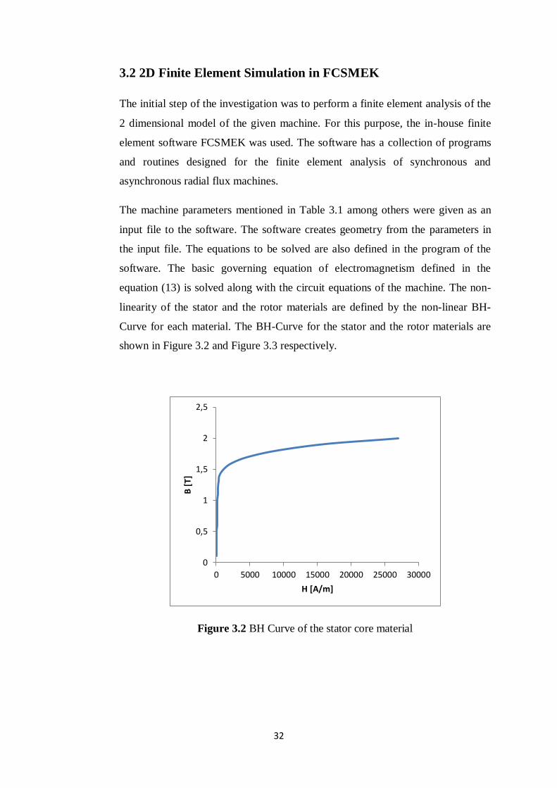
Curve for each material. The BH-Curve for the stator and the rotor materials are

shown in Figure 3.2 and Figure 3.3 respectively.

Figure 3.2 BH Curve of the stator core material

0

0,5

1

1,5

2

2,5

0 5000 10000 15000 20000 25000 30000

B [

T]

H [A/m]

33

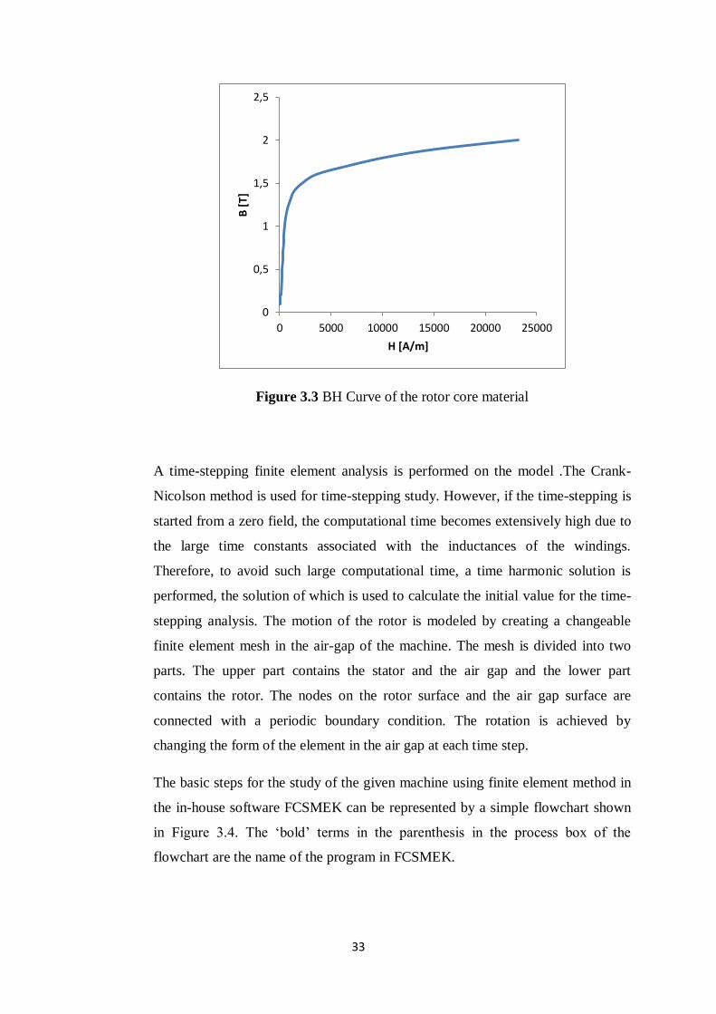
Figure 3.3 BH Curve of the rotor core material

A time-stepping finite element analysis is performed on the model .The Crank-

Nicolson method is used for time-stepping study. However, if the time-stepping is

started from a zero field, the computational time becomes extensively high due to

the large time constants associated with the inductances of the windings.

Therefore, to avoid such large computational time, a time harmonic solution is

performed, the solution of which is used to calculate the initial value for the time-

stepping analysis. The motion of the rotor is modeled by creating a changeable

finite element mesh in the air-gap of the machine. The mesh is divided into two

parts. The upper part contains the stator and the air gap and the lower part

contains the rotor. The nodes on the rotor surface and the air gap surface are

connected with a periodic boundary condition. The rotation is achieved by

changing the form of the element in the air gap at each time step.

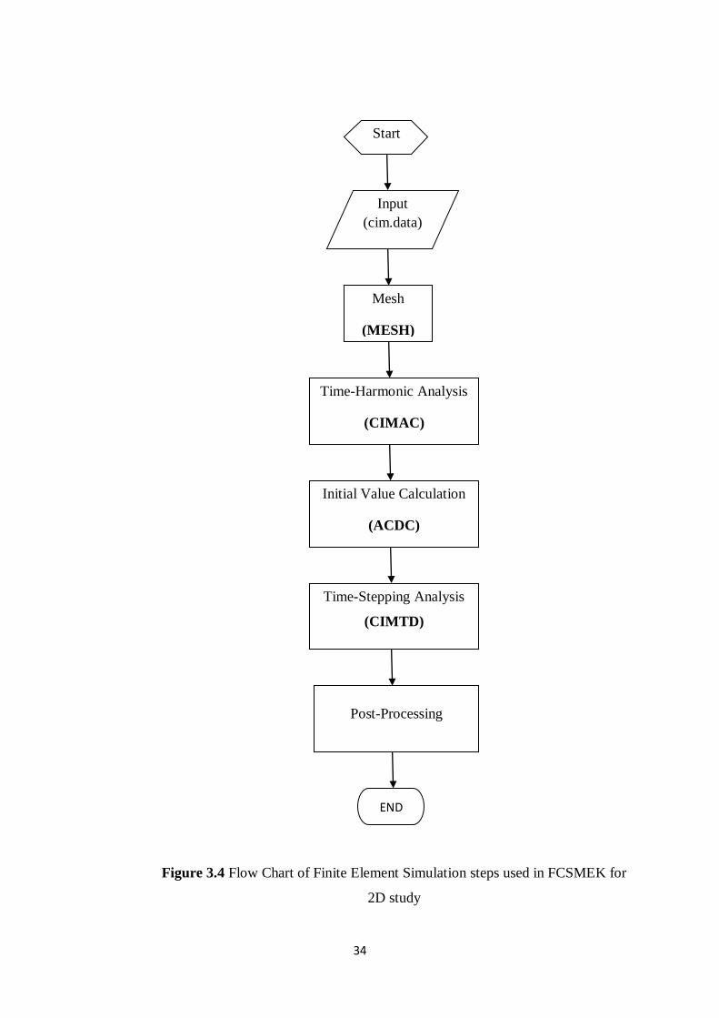
The basic steps for the study of the given machine using finite element method in

the in-house software FCSMEK can be represented by a simple flowchart shown

in Figure 3.4. The ‘bold’ terms in the parenthesis in the process box of the

flowchart are the name of the program in FCSMEK.

0

0,5

1

1,5

2

2,5

0 5000 10000 15000 20000 25000

B [

T]

H [A/m]

34

Figure 3.4 Flow Chart of Finite Element Simulation steps used in FCSMEK for

2D study

Start

Input

(cim.data)

Mesh

(MESH)

Time-Harmonic Analysis

(CIMAC)

Initial Value Calculation

(ACDC)

Time-Stepping Analysis

(CIMTD)

Post-Processing

END

35

3.3 Results from FCSMEK

Four periods of line frequency were simulated with 400 times steps per period of

line frequency. The total computational time was 260 seconds. Initially, the

MESH program generates a finite element mesh for the cross-sectional geometry

of the machine based on the data from the input file which contains the necessary

dimensions, slot numbers and slot indices. The program creates the smallest

possible symmetrical sector of the cross-section of the machine and draws the

triangular elements in it. A first order, changeable finite element mesh was made

in order to consider the rotation of the rotor, which is already explained in the

previous section. The resulting mesh consisted of 4032 elements and 2044 nodes.

There were 396 elements and 248 nodes in the stator and 3354 elements and 1796

nodes in the rotor. The air gap of the machine consisted of 282 finite elements.

The resulting mesh is shown in Figure 3.5.

Figure 3.5 Finite element mesh in the symmetric cross-section using FCSMEK

After creating the mesh in the two-dimensional geometry of the given machine,

the time-harmonic simulation was performed. The program uses Newton-Raphson

method to solve the non-linear system of equations obtained by the finite element

36

method. The results obtained from the time-harmonic analysis are shown in Table

3.2.

Table 3.2 Operating Characteristic of the machine obtained from the Time-

Harmonic Analysis

Parameter Value

Terminal voltage [V] 380

Supply frequency [Hz] 50

Line current [A] 14.98

Power factor 0.695

Slip [%] 5

Torque [Nm] 40.291

Rotation speed [rpm] 1425

Input Power [kW] 6.584

Shaft Power [kW] 6.095

Resistive stator loss [W] 438.2

Resistive rotor loss [W] 320.8

Core loss [W] 134.2

The magnetic flux density distribution resulting from the time stepping analysis of

the three-phase, 50 Hz, 380 V, star connected solid rotor induction machine at 5%

slip is shown in the Figure 3.6. The figure shows the magnetic flux distribution in

whole cross-section of the machine. The contours throughout the cross-section in

the Figure 3.6 are the equipotential lines. We can see that flux lines make a spiral

shape in the rotor. This can be because of the magnetic field produced by the

induced eddy currents in the rotor, which are circulating and produce a magnetic

field which are circulating around the path of the current. The characteristics of

the machine obtained from the time-stepping analysis are tabulated in Table 3.3.

37

Figure 3.6 Computed magnetic flux density distribution in the cross section of the

machine. Time Harmonic Analysis.

Figure 3.7 Computed magnetic flux density distribution in the computed region

along with the motion of the rotor shown. Time Stepping Analysis.

38

Table 3.3 Machine Characteristics resulting from TSA

Parameters Value

Terminal voltage [V] 380

Supply frequency [Hz] 50

Slip [%] 5

Terminal current [A] 14.665

Peak current [A] 20.710

Power factor 0.7165

Rotational speed [rpm] 1425

Air-gap torque [Nm] 35.445

Input Power [kW] 6.92

Shaft power [kW] 5.29

Air-gap flux density [T] 0.877

Current density in a stator slot [A/mm2] 2.88

Resistive stator loss [W] 420.04

Resistive rotor loss [W] 1173.52

Core loss in stator [W] 130.51

Core loss in rotor [W] 76.57

Total stator loss [W] 550.67

Total rotor loss [W] 1249.80

Total electromagnetic loss [W] 1800.48

Figure 3.6 shows the magnetic flux distribution in whole cross-section of the

machine. However, to reduce the computational time, only one symmetric sector

of the cross-section of the machine is taken into account for simulation. The

magnetic flux distribution in the region which is taken into account for

computation is shown in Figure 3.7. The motion of the rotor can also be

understood from this figure.

The three-phase current in the stator winding resulting from the simulation is

shown in Figure 3.8. The current density in the stator slot is used as a source in

the simulation carried out in the commercial software.

39

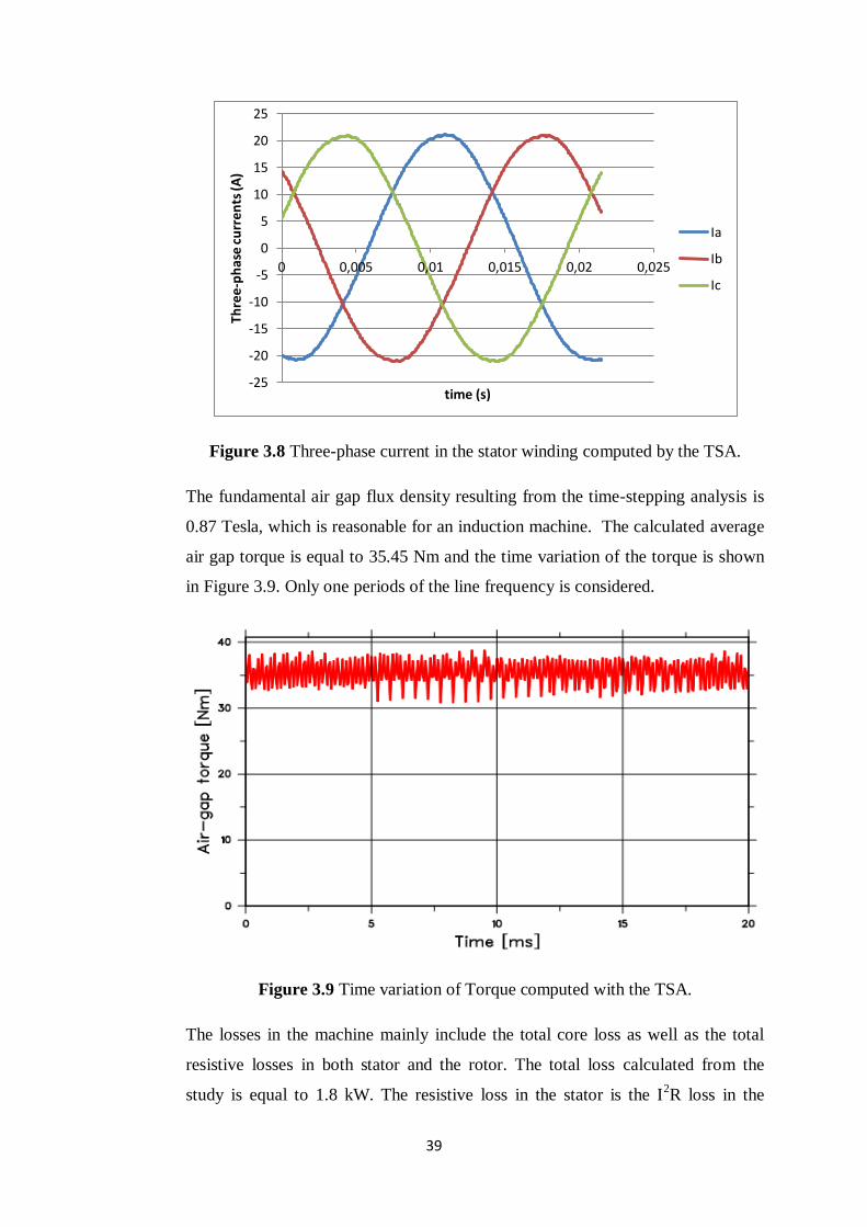
Figure 3.8 Three-phase current in the stator winding computed by the TSA.

The fundamental air gap flux density resulting from the time-stepping analysis is

0.87 Tesla, which is reasonable for an induction machine. The calculated average

air gap torque is equal to 35.45 Nm and the time variation of the torque is shown

in Figure 3.9. Only one periods of the line frequency is considered.

Figure 3.9 Time variation of Torque computed with the TSA.

The losses in the machine mainly include the total core loss as well as the total

resistive losses in both stator and the rotor. The total loss calculated from the

study is equal to 1.8 kW. The resistive loss in the stator is the I2R loss in the

-25

-20

-15

-10

-5

0

5

10

15

20

25

0 0,005 0,01 0,015 0,02 0,025

Thre

e-p

has

e c

urr

en

ts (A

)

time (s)

Ia

Ib

Ic

40

winding of the stator slot which is due to the flow of source current. However, the

given machine under study being a solid rotor machine does not consist of

conductor windings in the rotor. Therefore, the resistive loss that occurs in the

rotor is due to the currents that are induced in the rotor body. The conductivity of

the solid steel is involved. These induced currents are the eddy currents and the

losses due to these currents are the eddy current losses in the rotor of the machine.

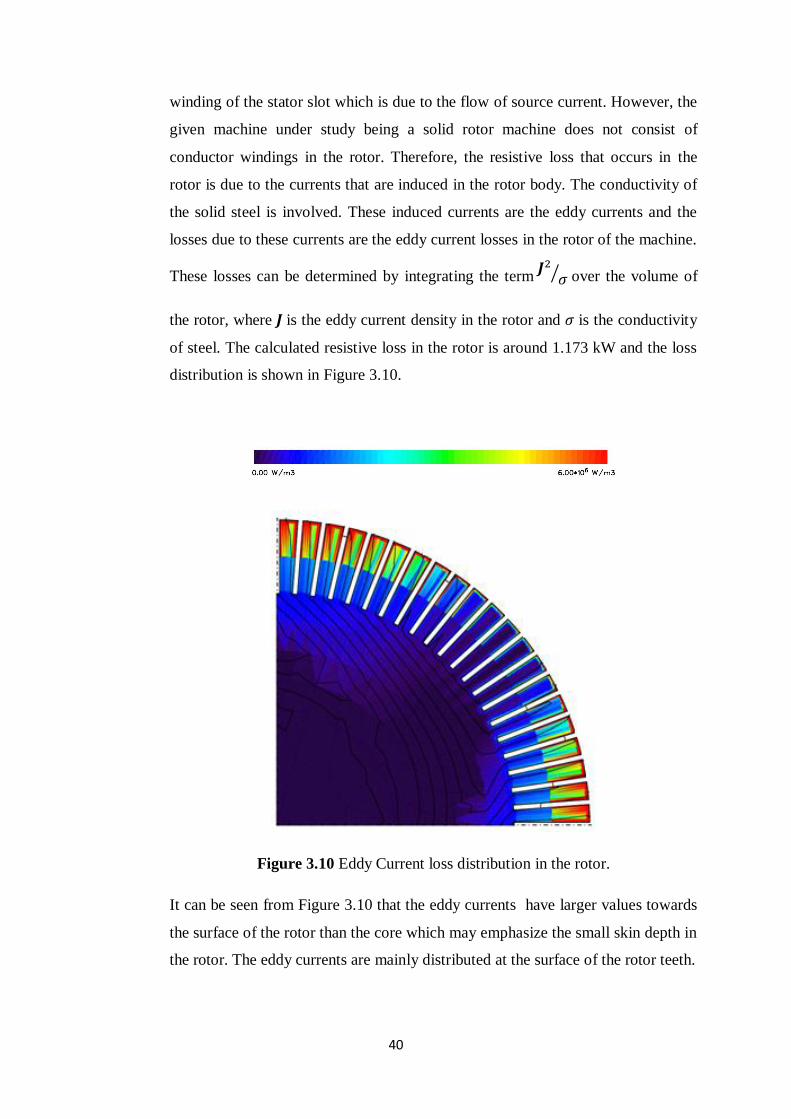
These losses can be determined by integrating the term

⁄ over the volume of

the rotor, where is the eddy current density in the rotor and is the conductivity

of steel. The calculated resistive loss in the rotor is around 1.173 kW and the loss

distribution is shown in Figure 3.10.

Figure 3.10 Eddy Current loss distribution in the rotor.

It can be seen from Figure 3.10 that the eddy currents have larger values towards

the surface of the rotor than the core which may emphasize the small skin depth in

the rotor. The eddy currents are mainly distributed at the surface of the rotor teeth.

41

3.4 3-D Physical Model

For the 2-D analysis in FCSMEK, the geometry was already defined in the

software through parameterization of different slot shapes. The geometrical

parameters of the two dimensional cross-section of the machine was defined in the

input file, according to which the program in the software created the mesh in the

geometry. The 2-D geometry of the machine is shown in Figure 3.1.

As stated earlier, due to the limitation of the in-house software FCSMEK, the 3-D

computation and analysis was performed in commercially available software.

However, the commercially available software did not have any pre-defined

machine geometry on which the study could be done. So, a 3-D geometrical

model of the machine had to be constructed. Since, this study dealt with the finite

element analysis in different dimensions of the same machine, each and every

geometrical dimension used for the construction of the 3-D model had to be equal

to the ones defined in the machine parameters of the in-house software FCSMEK

used for the 2-D simulation. This will not only assure for the different dimensions

of the same machine to be considered but also accounts for the reasonable

accuracy of the simulated results.

The 3-D model of the solid steel rotor induction machine used in the project was

constructed by using SolidWorks™ which is commercially available CAD

software. The length of the machine, inner and outer diameters of the stator and

the rotor, and the number of slots in the stator and rotor are given in Table 3.1.

The same parameters are used for designing the 3-D geometry.

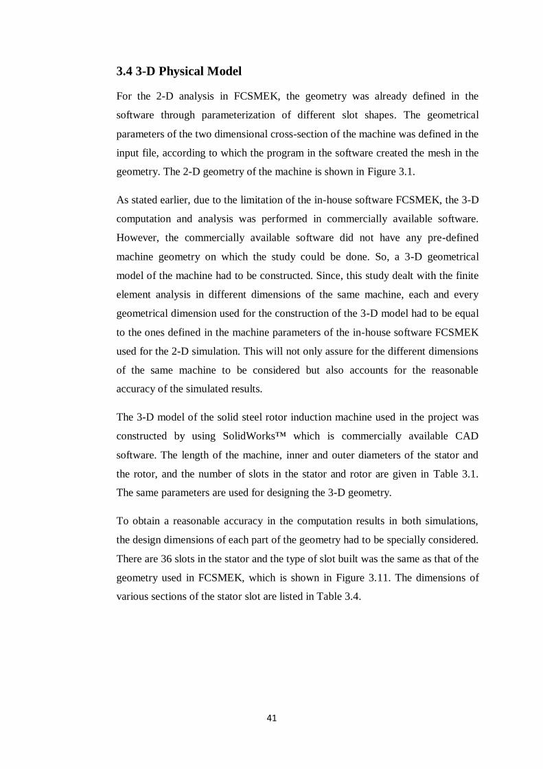
To obtain a reasonable accuracy in the computation results in both simulations,

the design dimensions of each part of the geometry had to be specially considered.

There are 36 slots in the stator and the type of slot built was the same as that of the

geometry used in FCSMEK, which is shown in Figure 3.11. The dimensions of

various sections of the stator slot are listed in Table 3.4.

42

Figure 3.11 Shape and dimension parameters of the stator slot.

Table 3.4 Dimensions of different sections of stator slot

Parameter Value

H1 [m] 0.0183

H11[m] 0.001

H13 [m] 0.0123

B11 [m] 0.003

B12 [m] 0.0053

B13 [m] 0.0075

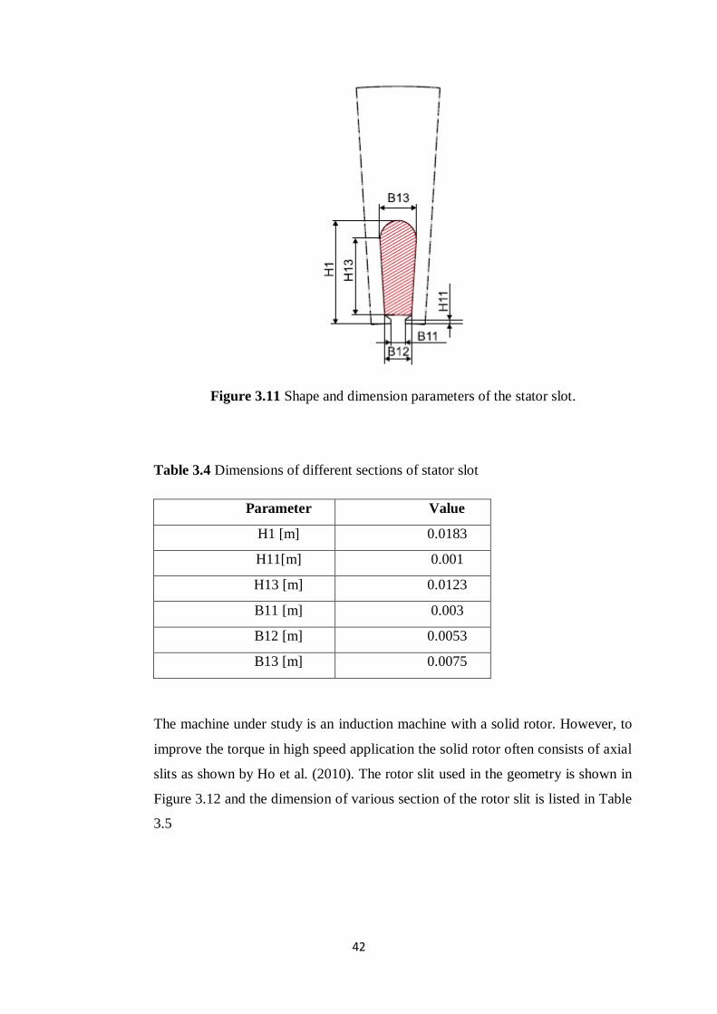
The machine under study is an induction machine with a solid rotor. However, to

improve the torque in high speed application the solid rotor often consists of axial

slits as shown by Ho et al. (2010). The rotor slit used in the geometry is shown in

Figure 3.12 and the dimension of various section of the rotor slit is listed in Table

3.5

43

Figure 3.12 Rotor Slit

Table 3.5 Dimensions of different sections of rotor slit

Parameter Value

H2 [m] 0.015

B2 [m] 0.001

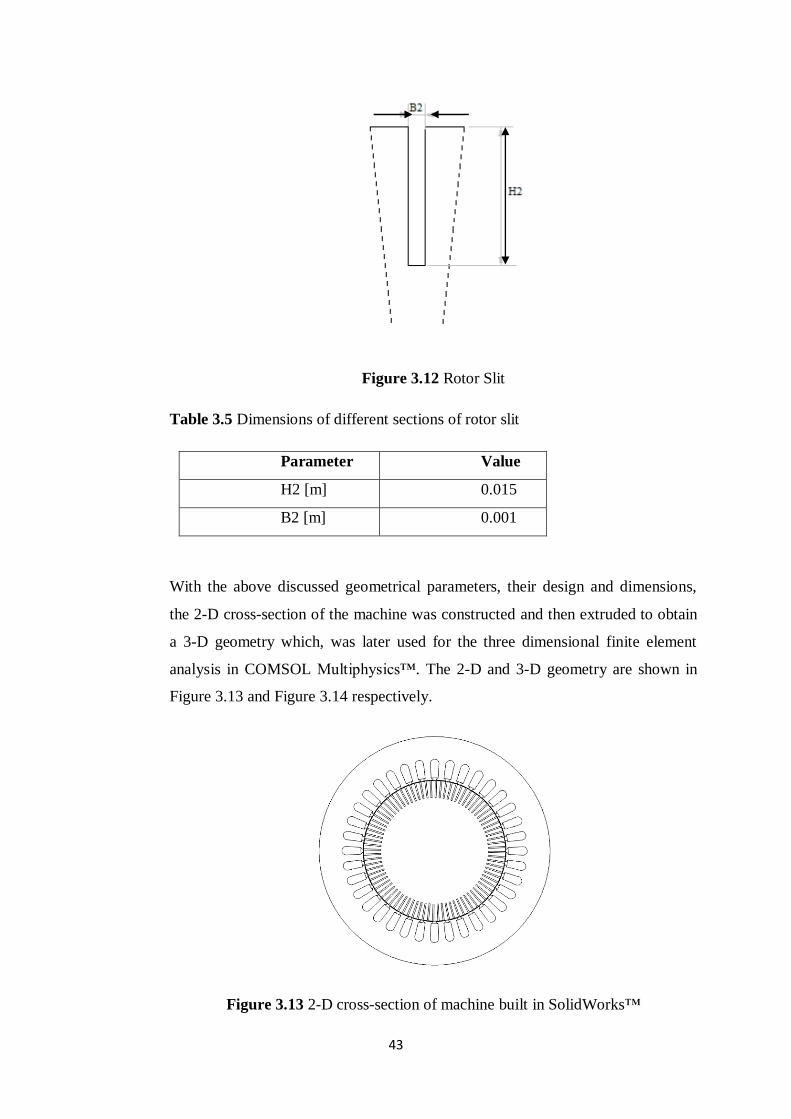
With the above discussed geometrical parameters, their design and dimensions,

the 2-D cross-section of the machine was constructed and then extruded to obtain

a 3-D geometry which, was later used for the three dimensional finite element

analysis in COMSOL Multiphysics™. The 2-D and 3-D geometry are shown in

Figure 3.13 and Figure 3.14 respectively.

Figure 3.13 2-D cross-section of machine built in SolidWorks™

44

Figure 3.14 The 3-D geometrical model

3.5 Data Transfer

In this thesis, we tried to use the solution obtained from FCSMEK as a source to

the simulation in COMSOL Multiphysics™. The main idea behind this was to

realize a coupled electromechanical model of the machine under study, in which

the 2D model of the machine was coupled with the 3D model of the rotor. For

this, the magnetic vector potential was used as the transferred variable. Our own

Matlab codes and subroutines were used for the entire data transfer process.

FCSMEK calculates the magnetic vector potential for each node in the mesh and

stores them along with other mesh information in a file called cim.fedat. A Matlab

code was used to read the file cim.fedat from FCSMEK to Matlab and store the

nodal values of the magnetic vector potential along with the node coordinates that

was stored in a database. Our idea was to run a 2D simulation of the same

machine and under same condition, and then read the mesh file from COMSOL

Multiphysics™ and then replace the coordinates of the nodal point and the

corresponding nodal values of the vector potential by those from FCSMEK. The

45

2D simulation in COMSOL Multiphysics™ is described later in this report. A

different routine was used to import the COMSOL Multiphysics™ mesh into

Matlab. The nodal coordinates and the nodal values of the magnetic vector

potential obtained from COMSOL Multiphysics™ were then replaced by those

obtained from FCSMEK manually. The modified mesh was then imported to

COMSOL Multiphysics™ again but the modified mesh was not supported due to

which the desired coupled model was not obtained. Moreover, the replacement of

the nodal coordinates and the corresponding nodal values of the vector potential in

the COMSOL Multiphysics™ mesh manually to modify the mesh was tedious and

time consuming. Therefore, this process of data transfer was regarded as

inappropriate.

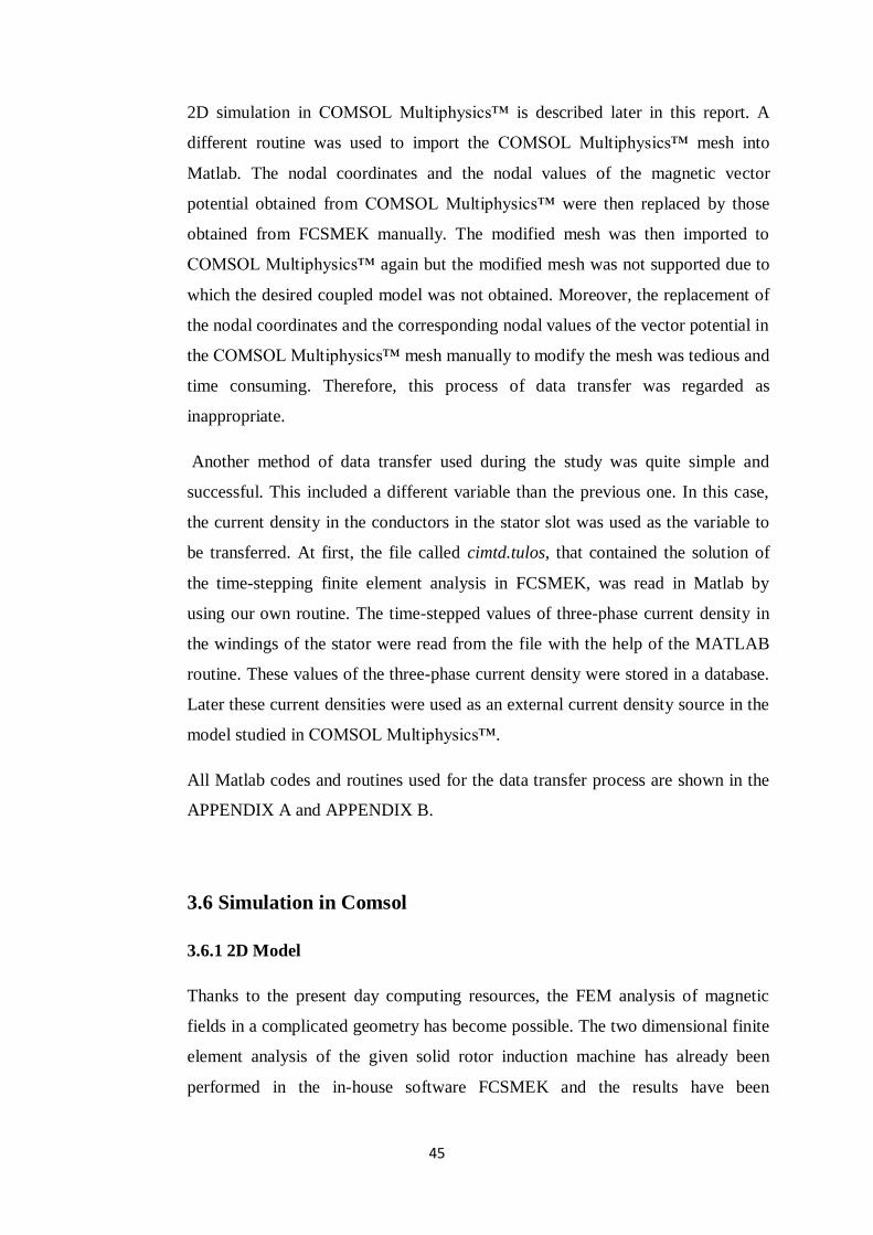
Another method of data transfer used during the study was quite simple and

successful. This included a different variable than the previous one. In this case,

the current density in the conductors in the stator slot was used as the variable to

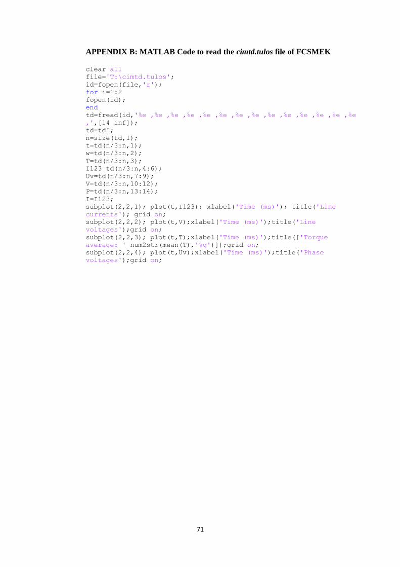
be transferred. At first, the file called cimtd.tulos, that contained the solution of

the time-stepping finite element analysis in FCSMEK, was read in Matlab by

using our own routine. The time-stepped values of three-phase current density in

the windings of the stator were read from the file with the help of the MATLAB

routine. These values of the three-phase current density were stored in a database.

Later these current densities were used as an external current density source in the

model studied in COMSOL Multiphysics™.

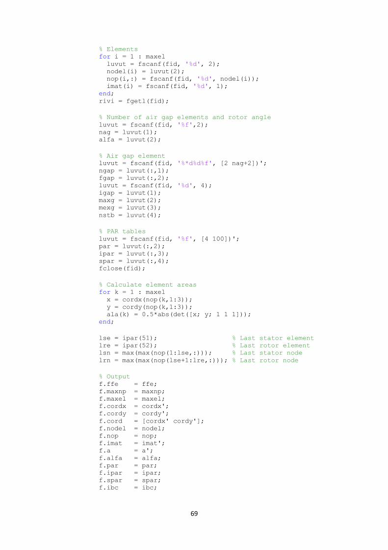
All Matlab codes and routines used for the data transfer process are shown in the

APPENDIX A and APPENDIX B.

3.6 Simulation in Comsol

3.6.1 2D Model

Thanks to the present day computing resources, the FEM analysis of magnetic

fields in a complicated geometry has become possible. The two dimensional finite

element analysis of the given solid rotor induction machine has already been

performed in the in-house software FCSMEK and the results have been

46

thoroughly analyzed. However, as an initial approach to use the commercially

available software, the two dimensional study of the machine was again

performed in COMSOL Multiphysics™.

The Maxwell equations and other governing equations for the calculation of eddy

currents have already been discussed in the previous chapter. The

formulation was used for the two dimensional finite element calculations of the

eddy currents. The governing equation for formulation of the eddy currents

used in this study is given in Equation (13).

This equation is solved only in the conduction region that is the region where the

eddy currents are present. But in the non-conducting region that is the region free

of eddy currents, the eddy current density given by

is assumed to be

zero. However, it is assumed that such region may include the current density due

to the source current. Thus the equation solved for non-eddy current region is

(22)

The conductivity of the rotor, which is the eddy current region in this case, is

considered to be constant. This consideration ensures that the gradient of the

electric scalar potential can be set to zero which has been shown by Rodger

(1983). This gives the equation to be solved in the conducting region to be as

given below.

(23)

As we have already mentioned, this study is a ‘coupled 2D-3D’ analysis of a solid

rotor induction machine in a sense that the solution of the two dimensional study

is used as the source in the three dimensional study. In this regard, the time-

stepped state values of current densities in the stator conductors obtained from the

two dimensional study in FCSMEK is used as the source current in the three

dimensional as well as two dimensional study in the COMSOL Multiphysics™.

So in the governing equation above that is Equation (13), the source current

density term is used as the source to the machine which is accounted by forcing

external current densities equal to the time-stepped three phase current densities in

the stator slot obtained from the solution in FCSMEK.

47

The default ‘magnetic insulation’ boundary condition of COMSOL

Multiphysics™ is used in the exterior boundary which sets the z-component of the

magnetic vector potential to zero at the boundary

(24)

The continuity of the normal component of the flux density and the tangential

component of the magnetic field strength is applied at the interface between the

conducting and the non-conducting regions.

The geometry of the machine used for the simulation in COMSOL

Multiphysics™ is built in commercially available CAD software which is already

described in Section 3.3. To understand the two dimensional magnetic flux

density distribution in the whole cross-section of the machine, the full pole pitch

of the machine was used for the simulation. The geometry built in the CAD

software was imported to COMSOL Multiphysics™. Since, the rotation of the

rotor had to be modeled, we needed a geometry such that the rotor section could

rotate. So, the imported geometry was re-processed to create two kind of

geometrical entities. The first kind included the fixed geometrical parts like the

stator core, stator slots and half of the radial length of the air gap and the second

kind included the rotating geometrical parts like the rotor and the other half of the

radial length of the air gap. The main reason for dividing the radial length of the

air gap into two parts, a rotating and a stationary is to simplify the modeling of the

rotation. The finalized geometry consisted of the assembly of these two parts. The

interface between the rotating and the stationary geometry is used as the interface

between the conducting and the non-conducting regions and a continuity pair

boundary condition is applied in this interface which assures the continuity of the

normal component of the flux density and the tangential component of the

magnetic field.

The material used in the simulation was the same as that used in the FCSMEK.

The material used for the stator core is Electrical Steel Sheet – Bochum

STABOLEC 260-50 A and that for the rotor core is Construction Steel (Ovako

520 L) whose properties were predefined in FCSMEK and the same was

prescribed in the material properties of the model. The stator core is a

48

magnetically non-linear medium and has zero conductivity whereas the rotor has

an isotropic conductivity of a finite value and is also a magnetically non-linear

medium. The magnetic non-linearity of the stator and the rotor core was applied

by using the non-linear BH curve for both the core materials. The non-linear BH

curve for the stator and the rotor core that are used in the model are shown in

Figure 3.2 and 3.3 respectively and are the same as the ones used in FCSMEK.

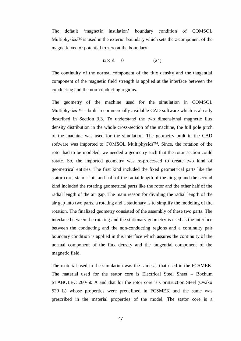
The finite element mesh plays a vital role in the FEM calculation especially in the

regard of both computational time and accuracy of the solution. Denser mesh

results into higher number of unknown variables but gives a solution that is more

likely to be accurate whereas a coarser mesh decreases the number of unknown

variables and thus the computational time but the results are more likely to deviate

from the accurate values. One another factor to be considered in meshing the

finite element model for eddy current calculation is the maximum element size for

the given skin depth. For a skin depth of 1 mm, the maximum size of the elements

should be less than 0.5 mm in that region which has also been discussed by Lin

(2009). In case of triangular elements the size of an element corresponds to the

length of the longest edge of the triangle. The mesh built for the 2D simulation

was such that the boundaries defined in the geometries are discretized

(approximately) into mesh edges, referred to as boundary elements (or edge

elements) by COMSOL Multiphysics™. The remaining geometry was meshed

with first order triangular elements. The meshed geometry is shown in Figure 3.15

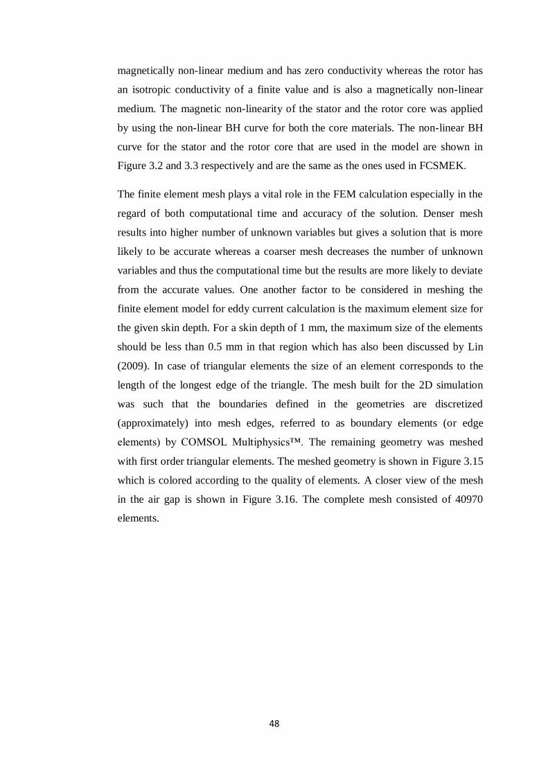
which is colored according to the quality of elements. A closer view of the mesh

in the air gap is shown in Figure 3.16. The complete mesh consisted of 40970

elements.

49

Figure 3.15 Part of the two dimensional mesh used in the 2D simulation with the

commercial software COMSOL Multiphysics™.

Figure 3.16 A closer view to the mesh near the air gap. The coloring is according

to the element shape quality.

50

COMSOL Multiphysics™ offers a variety of solvers for time harmonic as well as

time-stepping study. The time-stepping method is usually a very long process.

The machine model should be simulated tens of periods of line frequency to

achieve the steady state if the initial value field is assumed to be zero in time-

stepping computation. So, the model is first simulated by the time harmonic

method whose solution is then used as an initial state in the time stepping method.

This method will take a considerably smaller computation time and the steady

state can be achieved by simulating only few periods of line frequency.

One difficult aspect of the modeling of the rotating machinery is to model the

rotation. One way to model the rotation is to consider the rotor as a quasi or

pseudo-stationary object where it is fixed but the rotor conductivity is multiplied

by the per unit slip s for modeling the rotation as described by Arkkio (1987). But

this method is accurate only if the slip is 1. But Comsol has a feature where the

mesh of the rotating domain can be deformed with a prescribed mesh

displacement value. The main principle behind this feature is that we presribe a

set of equations that defines the displacement of the mesh of the domain in which

this feature has been used. So, in order to model the rotation of our model we used

the ‘Moving Mesh’ feature of the COMSOL Multiphysics™ in the rotating part of

the geometry that is the rotor and the equation for the mesh displacement in both

x-axis and y-axis was defined such that

(25)

(26)

Where,

is the speed of the machine in rps at corresponding slip

and are material frame coordinates.

The equations above ensure the displacement of the mesh of the rotating domain

in each time step. The machine was rotated at 5% slip which makes

. Thus the rotation in the machine is modeled by moving the mesh in

each time step.

51

3.6.2 3D model

Though the two dimensional finite element analysis of the electromagnetic field is

sufficient to study the approximate behavior of an electrical machine, some

phenomena can be well accounted only when the three dimensional finite element

analysis is done. So, a three dimensional model was built.

The three dimensional eddy current formulations have already been discussed in

the earlier chapter. In our model, we have used the equations of the

formulation where the magnetic vector potential is calculated in both the

conducting and the non-conducting region and the reduced electric scalar potential

is calculated in the conducting region only. The governing equations used for

the three dimensional formulation is the same as Equation (13) with vector

being a three dimensional vector. Even in this case, the reduced electric scalar

potential is set to zero. Therefore the basic formulation used can be considered

to be the magnetic vector potential formulation only. In the eddy current carrying

region that is the conducting region, equation (21) is solved and in the eddy

current free region where the eddy current density is assumed to be zero, equation

(15) is solved.

A coupled 3D model was realized in a sense that the solution of the two

dimensional study performed in the in-house software FCSMEK is used as the

source in the three dimensional study. This was possible by using the time-

stepped state values of three phase current densities in the stator conductors

obtained from the solution in FCSMEK as the source current density in the three

dimensional model in the COMSOL Multiphysics™. So the source current

density term in the equation (13) for the 3-D model is used as the source

current to the machine as it was done in the two dimensional study.

The default ‘magnetic insulation’ boundary condition of COMSOL

Multiphysics™ is used in the exterior boundary which sets the tangential

component of the magnetic vector potential zero at the boundary

(27)

52

The continuity of the normal component of the flux density and the tangential

component of the magnetic field is applied at the interface between the conducting

and the non-conducting region.

The three dimensional geometrical model of the machine is also built in

commercially available CAD software and the design process have been discussed

in Section 3.3. The full pole pitch of the machine was used for the simulation. Due

to the limited computing resources, the solution of the full length of the machine

was not possible. So, to simplify the model only a quarter of the total axial length

of the machine was simulated which significantly reduced the computation time.

However, this simplification does not consider the machine end effects which are

a major concern in 3-D eddy current problems. Therefore the result from this

simulation is subjected to deviate to some extent from the accurate results. To

account for the rotation of the rotor, the imported geometry was re-processed

similarly as the two dimensional geometry described in the previous section. The

finalized geometry consisted of the assembly of these two parts, a fixed part and a

rotating part. The interface between the rotating and the stationary geometry is

also used as the interface between the conducting and the non-conducting regions

which means that the electric scalar potential is also calculated in the lower part of

the air gap (the part included in the rotating geometry) and is equal to zero. A

continuity pair boundary condition is applied in this interface which assures the

continuity of the normal component of the flux density and the tangential

component of the magnetic field.

The material used in the 3D model is the same as that used in FCSMEK and also

for the 2-D simulation in COMSOL Multiphysics™. The material properties were

predefined in FCSMEK and are prescribed in the material properties of the model

in COMSOL Multiphysics™. The stator core is a magnetically non-linear medium

and has zero conductivity whereas the rotor has an isotropic conductivity of a

finite value and is also a magnetically non-linear medium. Since the conductivity

of the rotor is constant throughout the rotor body, there will be no potential

difference caused due to the electric charge in this region. Therefore the electric

scalar potential in the equation (13) becomes zero. So, the formulation used here

can be considered to be the magnetic vector potential formulation only. This

53

consideration decreases the number of dependent variables to be computed, thus

reducing the computing time.

The magnetic non-linearity of the stator and the rotor core was applied by using

the non-linear BH curve for both the core materials. The non-linear BH curve for

the stator and the rotor core that are used in the model are shown in Figure 3.12

and 3.13 respectively.

Meshing a 3D model needs a special care and attention. An improper mesh will

lead to inaccurate results and most of the time, COMSOL Multiphysics™ solver

find it difficult to solve the models with such improper meshes. Our 3D model has

a very thin air gap and meshing such thin domain requires good meshing skills.

The maximum element size must be less than the size of the domain which creates

a dense mesh of very small elements which may not lead to any solution as the

solver cannot solve it. The 3D geometry was first meshed with a first order

tetrahedral mesh. The 3D geometry meshed with the tetrahedral mesh is shown in

Figure 3.16. The mesh resulted in too high number of degree of freedoms to be

solved and was impossible to solve by the computer due to limited computer

memory (8, 16 or 32 GB).

Figure 3.17 Tetrahedral mesh in 3D geometry

54

Therefore an alternative way of meshing the 3D geometry was considered. In this

method, the 3D mesh was created in such a way that one of the axial cross-

sectional faces of the machine was meshed with a triangular mesh which was then

swept across the axial length to the other face. The complete mesh consisted of

32200 elements which resulted into lower DoFs relative to the tetrahedral mesh

which had 740013 elements. The complete swept mesh is shown in Figure 3.18.

The same solver used for the 2D simulation in COMSOL Multiphysics™

described earlier is also used for the 3D simulation. To avoid long computation

time, first the time-harmonic study is performed whose solution is then used as an

initial state in the time stepping method. A moving mesh is used in the rotating

Figure 3.18 Prism Mesh created by sweeping the triangular mesh

domain to realize the rotation of the rotor. The displacement of the mesh in x and

y axis are the same as that in Equation (25) and (26) and that in z-axis is zero

which is shown in Equation (28). These equation are prescribed in the rotating

domain.

0 (28)

, and are material frame coordinates.

55

These ensure the displacement of the three-dimensional mesh of the rotating

domain in each time step. The machine was rotated at 5% slip which makes

. Thus the rotation in the machine is modeled by the same method

as in the two-dimensional model by moving the mesh in each time step.

56

~ CHAPTER 4 ~

RESULTS AND DISCUSSIONS

Synopsis

This Chapter contains the results of both the two-dimensional and three-

dimensional study carried out in the COMSOL Multiphysics™. Different plots

and graphs are produced from the results and are presented in this chapter. Their

findings are also discussed in this chapter.

4.1 Results from 2-D Simulation

The two dimensional model built in COMSOL Multiphysics™ is described in

Section 3.5.1. Both time-harmonic and time dependent study is performed on the

model. The end-effect of the machine is neglected. The two dimensional finite

element mesh is shown in Figure 3.14 and 3.15. The mesh consisted of 20416

elements of type including triangular, edge and vertex elements. The number of

DoFs solved was 20932. Five periods of the line frequency with four hundreds

time-steps per period was simulated. The total computational time for the time-

dependent study of the two dimensional model with 20932 DoFs was 4134

seconds. The simulation was performed on a computer with Intel® Core(T)2

Quad CPU with 8 GB RAM.

The flux density distribution obtained from the time-dependent study is shown in

Figure 4.1. We can see that in the stator more flux is concentrated in the stator

teeth near the poles and in the stator yoke around the inter-polar regions. In the

rotor, the flux is more concentrated near to the surface of the rotor. This is because

of the fact that the flux penetration into the conducting rotor material causes the

eddy currents which again tends to prevent the flux penetration.

57

Figure 4.1 Magnetic flux density distribution and the flux lines as computed with

TSA in the COMSOL Multiphysics™ software.

The axial slits in the solid rotor form a path for the eddy currents to flow from one

rotor end to the other through the rotor teeth between the slits. A circulating

magnetic flux is created by the currents that flow through the rotor teeth. So, the

flux lines make a magnetic spiral or curl shape in the solid rotor with axial slits.

The resulting flux lines are shown along with the magnetic flux density

distribution in Figure 4.1.

Figure 4.2 shows the eddy currents density that is induced in the solid rotor

resulting from the time-dependent study. We can see that the induced currents are

mainly distributed in the rotor teeth and penetrate to a very low level inside the

rotor. This may be due to small skin depth of the rotor. It can also be understood

from the same figure that the eddy current is flowing along the axial direction that

is along the z-direction. From the figure, only the distribution of eddy currents

can be seen, but the flow of the current can be well visualized in the three

dimensional model.

58

Figure 4.2 Eddy current density distribution

The time variation of the torque calculated from the 2-D simulation with

COMSOL Multiphysics™ is shown in the figure 4.3.

The average air gap torque of the machine is higher than that calculated in

FCSMEK. The electromagnetic torque is calculated using the Maxwell’s stress

tensor and is given by the surface integral over the closed surface S located in the

air gap.

∮ (29)

Where, is the Maxwell’s stress tensor and r is the position vector directed from

the rotor origin to the point of calculation. In 2-D model the surface integral is

reduced to the line integral along the air gap.

59

Figure 4.3 Torque variation resulting from 2-D simulation in COMSOL

Multiphyscis™

4.2 Results from 3-D Simulation

The three dimensional model built in COMSOL Multiphysics™ is described in

Section 3.5.1. Both time-harmonic and time dependent study is performed on the

3-D model too. Taking both the active region and the end region of the machine

into consideration for the model would increase the complexity of the problem.

So, only the active region of the machine was taken into account and the end-

effect of the machine is neglected. This will however produce a result that is

subjected to deviate to some extent from the accurate result as discussed in earlier

chapter. The 3-D mesh is shown in Figure 3.17. The complete mesh consisted of

32200 elements which include triangular, prism, quadrilateral, edge and vertex

elements. To reduce the number of unknown variables, only one-fourth of the

axial length of the machine was simulated. The number of Degree of Freedoms

solved was 90622. Five periods of the line frequency with four hundreds steps per

period were simulated. The total computational time for the time-dependent study

of the three dimensional model in a computer with Intel® Xeon® CPU with 16

GB RAM for 90622 DoFs was 19853 seconds.

60

Figure 4.4 Three-dimensional flux density distribution computed with the 3D

model in COMSOL Multiphysics™.

The three-dimensional flux density distribution in the machine is shown in Figure

4.4. The flux seems to be concentrated in the stator yoke in the inter-polar region

and in the stator teeth near the poles in the stator. In the rotor, the flux is more

concentrated near the surface of the rotor because of the fact that the induced

current in the conducting rotor tends to oppose the flux penetration into it. The

result of the 3-D simulation, in terms of the computed magnetic flux density is

quite different. We can see that the flux density is quite high compared to the 2-D

model.

The flow of the eddy currents through the rotor bars between the slits from one

end of the rotor to the other end can be clearly visualized in the three-dimensional

model. The eddy current density distribution and the flow of current from one end

of the rotor to the other can be seen from Figure 4.5.

61

Figure 4.5 Eddy current density distribution and the flow of eddy currents (z-

component)

A closer view of the flow of the eddy currents is presented in Figure 4.6. Currents

circulate mainly through the surface of the rotor bars. It flows from one end to the

other at one pole of the machine and returns back similarly from the other end at

the adjacent pole. However, the looping of the currents at the end faces of the

rotor could not be accurately modeled.

The torque calculated from the 3-D simulation is plotted in Figure 4.7. The torque

is calculated using the Maxwell’s stress tensor.

62

Figure 4.6 Computed z-component of the Eddy Currents.

Figure 4.7 Torque variation resulting from 3-D simulation in COMSOL

Multphysics™

63

~ CHAPTER 5 ~

CONCLUSION

The finite element method was used to compute the eddy currents in both two

dimensional and the three dimensional model of a solid rotor induction machine.

A three phase, 50 Hz, 380 V, star connected, 7.5 kW solid steel rotor induction

machine was considered for the study. At first the two dimensional model of the

machine was simulated in the in-house software FCSMEK. The eddy current was

computed and the distribution of the eddy currents in the rotor teeth and rotor

surface was studied. A three dimensional finite element model of the same

machine was built in commercial software Comsol Multiphysics™. But before

modeling the three dimensional model, a two dimensional model was built in

Comsol Multiphysics™ as an initial approach to use the software and be able to

compare the two different 2D approaches. Both the two dimensional and three

dimensional model in Comsol Multiphysics™ was built in such a way that they

were coupled with the model in FCSMEK. The original idea behind the coupled

model was such that the computed magnetic vector potential in the rotor surface

from the 2-D simulation in FCSMEK would be stored and then used as an initial

value in one of the rotor surface in the 3-D model in Comsol Multiphysics™ and

then extruded along the axial length of the machine with a suitable interpolation.

Since, only the study of the rotor would be sufficient to accurately model the eddy

currents, without the need of the 3-D model of the stator, this type of coupled

model would have a great advantage in terms of simplicity and the reduction of

computational time.

This kind of coupled model was tried to build in Comsol Multiphysics™, but the

nodal values of the magnetic vector potential could not be transferred to the nodes

of the rotor mesh in Comsol Multiphysics™. Comsol Multiphysics™ did not

support any alteration of its finite element mesh externally. So, an alternative way

was chosen. A coupled model was however realized, but the transferred variable

was the time-stepped stator winding current density. The time-stepped solution of

64

the stator winding current density was used as a source to the windings in both the

2-D and the 3-D model in Comsol Multiphysics™. The formulation was

used for the eddy current calculation. The physical model of the machine was

built in a CAD software called SolidWorks™ and then exported to Comsol

Multiphysics™. The results from all the simulations are shown in the earlier

chapters.

Although it was expected that the coupled model reduces the computational

time,the results did not match the expectations. The results from the FCSMEK

and Comsol Multiphysics™ differ quite considerably, especially in terms of the

torque. The magnetic flux density distribution in the machine computed from the

2-D model in Comsol Multiphysics™ is similar to the flux density distribution

computed from FCSMEK. However, the average flux density in the air gap is

comparatively lower than that calculated in FCSMEK. The magnetic flux density

computed in the 3-D model is slightly higher than that in the 2-D models. The

advantage of 3-D model is that the field distribution in the actual machine can be

visualized. The eddy current distribution in the rotor surface is plotted from the

results of each simulation. From the 2-D plot of the eddy current distribution, it

can be seen that the eddy current are mostly distributed in the rotor teeth. The

eddy currents circulate through the surface of the rotor teeth, which can be clearly

noticed in the 3-D eddy current plots. The eddy current flows from one end of the

rotor to the other end through the axial surface of the rotor teeth and the radial

surface provides the return path for it. However, the looping of the current near

the end surface of the rotor could not be obtained. This is the major limitation of

the model built in COMSOL Multiphysic™ in this thesis. The torque calculation

in COMSOL Multiphysics™ when compared to that in FCSMEK differs quite

considerably. It is seen that the torque calculated in both 2-D and the 3-D model

in COMSOL Multiphysics™ is considerably high than that calculated in

FCSMEK, around 2.5 and 2.2 times.

Thus, the eddy current was computed using both 2-D and 3-D Finite Element

Method. A coupled model was studied by using the solution from results of 2-D

simulation in the in-house software as a source to the 2-D and 3-D model in

commercial software COMSOL Multiphysics™. Since the experimental results

65

for the machine were not available, the simulated results could not be validated.

The major limitation of the coupled model discussed here in this thesis is that the

looping of the eddy currents near the end region of the rotor could not be

obtained. So, this model can be given additional work in future to address this

limitation. Also the computational time of the coupled model was more than

expected.

66

References:

A. Arkkio, (1987). Analysis of Induction Motor Based on the Numerical Solution

of the Magnetic Field and Circuit Equations. Acta Polytechnica Scandinavica, 59

A. Arkkio, (1990). Finite Element Analysis of Cage Induction Motors fed by

Static Frequency Converters, IEEE Trans. Magn., 26(2):2-5.

B. Brunelli, D. Casadei, U. Reggiani, G. Serra, (1983). Transient and Steady-State

Behavior of Solid Rotor Induction Machines, IEEE Trans. Magn., 19(6):2650-

2654.

B. Davat, Z. Ren, M. Lajoie-Mazenc, (1985). The Movement in Field Modeling.

IEEE Trans. Magn. 21(6):2296-2298.

D. Rodger, (1983). Finite Element Method for Calculating Power Frequency 3-

Dimensional Electromagnetic Field Distributions. In Proc. IEE, Science, 130

J. D. Jackson, (1999). Classical Electrodynamics. 3rd

ed. New York, NY, John

Wiley and Sons Inc.

J. Gieras, (1995). Solid-Rotor Induction Motor Design, pages 293-298. In

Engelmann, R., Middendorf, W. Handbook of Electric Motors, Marcel Dekker

Inc., New York.

J. F. Gieras, J. Saari, (2010). Performance Calculation for a High Speed Solid-

Rotor Induction Motor. In Proc. 36th Annual Conference on IEEE Industrial

Electronics Society, pages 1748-1753, Glendale, AZ, USA.

J. Huppunen, (2004). High-Speed Solid-Rotor Induction Machine –

Electromagnetic Calculation and Design. Doctoral Dissertation, Lappeenranta

University of Technology, Lappenranta, Finland.

J. Luomi, (1993). Finite Element Methods for Electrical Machines. Lecture Notes,

Chalmers Universtiy of Technology, Göteborg, Sweden.

M. J. Balchin, J. A. M. Davidson, (1983). 3-Dimensional Eddy-Current

Calculation by the Network Method Formulation Using Magnetic Scalar Potential

for Nonconducting Regions. In Proc. IEE, A Physical Science, Measurement and

Instrumentation, Management and Education, Reviews, 130(2):88.

M. J. Islam, A. Arkkio, (2008). Time-Stepping Finite-Element Analysis of Eddy

Currents in the Form-Wound Stator Winding of a Cage Induction Motor Supplied

from a Sinusoidal Voltage Source. In Proc. IET Electrical Power Applications,

2(4):256-265

67

O. Biro, K. Preis, (1989). On The Use of the Magnetic Vector Potential in the

Finite-Element Analysis of Three-Dimensional Eddy Currents. IEEE Trans.

Magn, 25(4):3145-3159.

O. Biro, K. Preis, (1990). Finite Element Analysis of 3-D Eddy Currents. IEEE

Trans. Magn., 26(2):418-423.

P. Dziwniel, F. Piriou, J. P. Ducreux, P. Thomas, (1999). A Time-Stepped 2D-3D

Finite Element Method for Induction Motors with Skewed Slots Modeling. IEEE

Trans. Magn., 35(3):262-1265.

P. J. Leonard, D. Rodger, (1988). Finite Element Scheme for Transient 3D Eddy

Current Analysis. IEEE Trans. Magn., 24:90.

S. L. Ho, Niu. Shuangxia, W. N. Fu, (2010). A Novel Solid-Rotor Induction

Motor with Skewed Slits in Radial and Axial Directions and Its Performance

Analysis Using Finite Element Method. IEEE Trans. App. Superconductivity,

20(3):1089-1092.

S. Kanerva, (2001). Data Transfer Methodology Between a FEM Program and a

System Simulator. In Proc. 5th

Int. Conf. Electrical Machines and Systems.

Vol(2):1121-1124).

T. Aho, J. Nerg, J. Pyrhonen, (2006). The Effect of the Number of Rotor Slits on

the Performance Characteristics of Medium-Speed Solid Rotor Induction motor.

In Proc. 3rd

IET Int. Conf. Power Electronics, Machines and Drives, pages 515-

519, Dublin, Ireland.

T. Kikuchi, T. Kenjo, (1997). A unique Desk-top Electrical Machinery Laboratory

for the Mechatronics Age. IEEE Trans. Education, 40(4).

T. Yang, L. Zhou, W. Jiang, (2008). Calculation of Eddy Current Losses in a

Solid-Rotor Cage Induction Motor by Finite Element Analysis. In Proc. Int.

Conf. Electrical Machines and Systems, pages 3656-3659, Wuhan, China.

W. Muller, A. Knoblauch, (1985). A Method for Numerical Calculation of 3D

Eddy-Currents. IEEE Trans. Magn., 21(6).

68

APPENDIX

APPENDIX A: MATLAB Codes used to read the cim.fedat file of FSCMEK

function f = readCimFedat(file) % Read FEM data from cim.fedat

if nargin == 0 clc; file = 'T:\results'; end; if file(end) == '\' file = [file 'cim.fedat']; end;

fid = fopen(file); % fgetl(fid); % luvut = fscanf(fid, '%d',5);

% Number of nodes and elements maxnp = luvut(1); maxel = luvut(2); nfe = luvut(3); npm = luvut(4); ndb = luvut(5);

% HPER and pituus luvut = fscanf(fid, '%f', 2); hper = luvut(1); pituus = luvut(2); fgetl(fid);

% Read FFE table line = fgetl(fid); luvut = sscanf(line, '%f'); ffe= []; while length(luvut) < 6 ffe(end+1,1:5) = luvut(1:5); line = fgetl(fid); luvut = sscanf(line, '%f'); ffe(end,6:9) = luvut(1:4); line = fgetl(fid); luvut = sscanf(line, '%f'); end;

% Node coordinates cordx(1) = luvut(2); cordy(1) = luvut(3); a(1) = luvut(4); ibc(1) = luvut(end); luvut = fscanf(fid, '%d%f%f%f%f%d', [6 maxnp-1])'; cordx(2:maxnp) = luvut(:,2); cordy(2:maxnp) = luvut(:,3); a(2:maxnp) = luvut(:,4); ibc(2:maxnp) = luvut(:,end);

69

% Elements for i = 1 : maxel luvut = fscanf(fid, '%d', 2); nodel(i) = luvut(2); nop(i,:) = fscanf(fid, '%d', nodel(i)); imat(i) = fscanf(fid, '%d', 1); end; rivi = fgetl(fid);

% Number of air gap elements and rotor angle luvut = fscanf(fid, '%f',2); nag = luvut(1); alfa = luvut(2);

% Air gap element luvut = fscanf(fid, '%*d%d%f', [2 nag+2])'; ngap = luvut(:,1); fgap = luvut(:,2); luvut = fscanf(fid, '%d', 4); igap = luvut(1); maxg = luvut(2); mexg = luvut(3); nstb = luvut(4);

% PAR tables luvut = fscanf(fid, '%f', [4 100])'; par = luvut(:,2); ipar = luvut(:,3); spar = luvut(:,4); fclose(fid);

% Calculate element areas for k = 1 : maxel x = cordx(nop(k,1:3)); y = cordy(nop(k,1:3)); ala(k) = 0.5*abs(det([x; y; 1 1 1])); end;

lse = ipar(51); % Last stator element lre = ipar(52); % Last rotor element lsn = max(max(nop(1:lse,:))); % Last stator node lrn = max(max(nop(lse+1:lre,:))); % Last rotor node

% Output f.ffe = ffe; f.maxnp = maxnp; f.maxel = maxel; f.cordx = cordx'; f.cordy = cordy'; f.cord = [cordx' cordy']; f.nodel = nodel; f.nop = nop; f.imat = imat'; f.a = a'; f.alfa = alfa; f.par = par; f.ipar = ipar; f.spar = spar; f.ibc = ibc;

70

f.ala = ala; f.lse = lse; f.lre = lre; f.lsn = lsn; f.lrn = lrn; f.nag = nag; f.ngap = ngap; f.fgap = fgap; f.igap = igap; f.maxg = maxg; f.mexg = mexg; f.nstb = nstb; f.nfe = nfe; f.npm = npm; f.ndb = ndb; f.hper = hper; f.pituus = pituus;

71

APPENDIX B: MATLAB Code to read the cimtd.tulos file of FCSMEK

clear all file='T:\cimtd.tulos'; id=fopen(file,'r'); for i=1:2 fopen(id); end td=fread(id,'%e ,%e ,%e ,%e ,%e ,%e ,%e ,%e ,%e ,%e ,%e ,%e ,%e ,%e

,',[14 inf]); td=td'; n=size(td,1); t=td(n/3:n,1); w=td(n/3:n,2); T=td(n/3:n,3); I123=td(n/3:n,4:6); Uv=td(n/3:n,7:9); V=td(n/3:n,10:12); P=td(n/3:n,13:14); I=I123; subplot(2,2,1); plot(t,I123); xlabel('Time (ms)'); title('Line

currents'); grid on; subplot(2,2,2); plot(t,V);xlabel('Time (ms)');title('Line

voltages');grid on; subplot(2,2,3); plot(t,T);xlabel('Time (ms)');title(['Torque

average: ' num2str(mean(T),'%g')]);grid on; subplot(2,2,4); plot(t,Uv);xlabel('Time (ms)');title('Phase

voltages');grid on;