Beyond DFT-Landauer Quantum Transport: Ab Initio GW-NEGF

in Nano- and Molecular ElectronicsPierre Darancet, Tonatiuh Rangel, Andrea Ferretti,

Paolo Emilio Trevisanutto, Didier Mayou,

Gian-Marco Rignanese, Valerio OlevanoInstitut Néel, CNRS Grenoble

European Theoretical Spectroscopy Facility

Outline:1. Quantum-Transport problem2. DFT-Landauer Formalism3. Non-Equilibrium Green's Functions (NEGF) Theory4. e-e scattering effects and GW5. Results:

• Au monoatomic chain• BDA / BDT@gold

6. Conclusions

Molecular and NanoElectronicsQuantum Transport

Both an Experimental, a Technologicaland a Theoretical Challenge!

Nanoscale Electronics Devices

Real Theoretical challenge: predict ab initio the I/V Characteristics

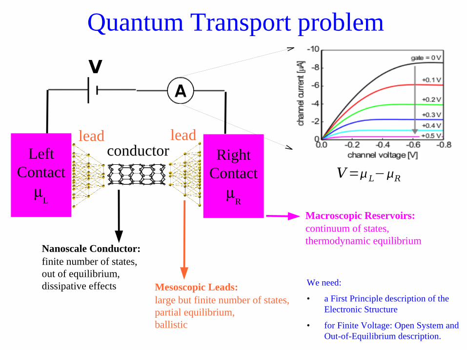
Quantum Transport problem

LeftContact

L

V

V=L−R

RightContact

R

lead leadconductor

Nanoscale Conductor:finite number of states,out of equilibrium,dissipative effects Mesoscopic Leads:

large but finite number of states,partial equilibrium,ballistic

Macroscopic Reservoirs:continuum of states,thermodynamic equilibrium

We need:

• a First Principle description of the Electronic Structure

• for Finite Voltage: Open System and Out-of-Equilibrium description.

Landauer Theory

C =2e²hM T

[eV ]

Landauer Formula

S. Datta, (1995)R. Landauer, IBMJ. Res. Dev. (1957)

LeftContact

µL

RightContact

µR

lead leadconductor

T

state-of-the-art

Landauer Theory C =2e²hM T

Landauer FormulaT Transmittance

1) Calculated via a standard Quantum Mechanics approach:

H=

T R Transmission and Reflection coefficients

Example: potential barrier

2) Or via a Green's function approach

−H G r ,r ' ,=r ,r '

probability that an electron of energy εinjected in r be transmitted in r' r r'

Landauer Formula in Green's functions

Gc=−H c− l−r −1

conductor-lead coupling

conductorGreen's functions

l=H lc† glH lc

r=H crgrH cr†

gl , r=−H l , r −1

l , r=i[l ,rr−l , r

a]

G l Glc G lcr

Gcl Gc Gcr

Grcl Grc Gr=−Hl −H lc 0

−H lc† −Hc −H cr

0 −Hcr†

−H r −1

lead self-energies

leads bulk Green's functions

T=tr [lGcrrGc

a] Fisher-Lee relation

conductor

leads

c rl

Landauer on top of DFT

H=H l H lc 0

H lc† H c Hcr

0 Hcr† Hr

What to take for the hamiltonian?

the DFT Kohn-Sham hamiltonian!

conductor

leads

c rl

(represented on a real space basis like atomic orbitals, Wannier functions, etc.)

PtH2

K.S. Thygesen K.W. Jakobsen,Chem. Phys. (2005)

Depletion ofPt d states

EXP (break junctions): C(0) ~ 1 [G0=2e2/h]

R.H.M. Smit et al, Nature 419, 906 (2002)

Example of Landauer conductance

Landauer approach

Correctly describes:

✔ Contact Resistance

✔ Scattering on Defects, Impurities

✔ Non-commensurability patterns

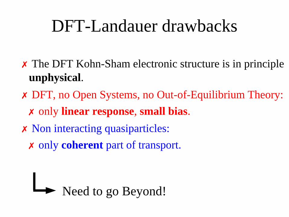
DFT-Landauer drawbacks

✗ The DFT Kohn-Sham electronic structure is in principle unphysical.

✗ DFT, no Open Systems, no Out-of-Equilibrium Theory:

✗ only linear response, small bias.

✗ Non interacting quasiparticles:

✗ only coherent part of transport.

Need to go Beyond!

Beyond LB-DFT:2 Possibilities

• TDDFT for Quantum Transport✔promising possibility

✗ need a suitable approx for xc

✗ cannot deal with open systems

• NEGF (NonEquilibrium Green's Function theory)✔ full access to all observables

✔ it has maybe a more intuitive physical meaning

Non-Equilibrium Green's Function Theory (NEGF)

(improperly called Keldysh theory)

Much more complete framework, allows to deal with:

• Many-Body description of incoherent transport (electron-electron interaction, electronic correlations and also electron-phonon);

• Out-of-Equilibrium situation;

• Access to Transient response (beyond Steady-State);

• Reduces to Landauer for coherent transport.

The theory is due to the works of Schwinger, Baym, Kadanoff and Keldysh

Many-Body Finite-Temperatureformalism

H= T V W

H = e−H

tr [e− H ]statistical weight

observable

hamiltonianmany-body

o=∑i e−E i ⟨ i∣o∣i ⟩

∑i e−Ei

=tr [ H o]

Valerio Olevano, CNRS Grenoble

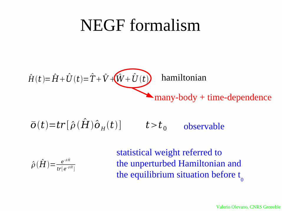
NEGF formalism

H t = H U t = T V W U t

ot =tr [ H oH t ] tt0

H = e−H

tr [e− H ]

statistical weight referred tothe unperturbed Hamiltonian andthe equilibrium situation before t

0

observable

hamiltonian

many-body + time-dependence

Valerio Olevano, CNRS Grenoble

Time Contour

ot=tr [ s t0−i , t0 s t0 ,t o t s t ,t 0 ]

tr [ s t0−i , t0 ]

evolution operator

Heisenberg representationoH t = st0 ,t ot st , t0

st ,t0=T {exp −i∫t 0t dt ' H t ' }

st0−i , t0=e− H

ot =tr [TC [exp−i∫Cdt ' H t ' o t ]]

tr [T C[exp−i∫C dt ' H t ' ]]

trick to put the equilibrium weightinto the evolution

Valerio Olevano, CNRS Grenoble

Contour and Perturbation Theory

• To recover perturbation theory (Wick's theorem, Feynman diagrams, etc.) you have to declare the Green's function and all the quantities on the Closed Contour.

Gco x1, x2=−iT c {H x1H† x2}

contour ordered Green's function

Gcox1, x2=

Gt ox1, x2 t1,t2∈C

Gatox1, x2 t1,t2∈C∧

G x1 , x2 t1∈C , t2∈C∧

G x1 , x2 t1∈C∧ ,t2∈C{

Valerio Olevano, CNRS Grenoble

Keldysh Formulation

GkoG=G11 G12

G21 G22

G11x1,x2=Gt ox1,x2

G12x1,x2=Gx1,x2

G21x1,x2=G x1,x2

G22x1,x2=Gatox1,x2

G '= 0 Ga

Gr Gk Gk=G

G

G ''=Gr Gk

0 Ga

Keldysh formulation

Larkin-Ovchinnikovformulation

Keldysh Green's function

Schwinger-Keldyshcontour

Valerio Olevano, CNRS Grenoble

Green's and Correlation FunctionsGr

G

G

−iG = f FD A

iG =[1− f FD ]A

Gt o=Gr

G

A=iGr−Ga

Out of Equilibriumwe need to introduceat least three unrelated“Green's” functions.

At Equilibrium the Correlationfunctions are related to the Green's function through the Fermi-Dirac distribution.

Spectral Function

Once we know the Green's and the Correlation functions,the problem is solved!They contain all the physics!

hole and electrondistribution functions

Valerio Olevano, CNRS Grenoble

NEGF Fundamental KineticEquations

Gr=[−H c−

r]−1

G =Gr

Ga

G =Gr

Ga

Caveat!: in case we want to consider also the transient,then we should add another term to these equations:

G =Gr

Ga

1GrrG0

1aGa Keldysh equation

Valerio Olevano, CNRS Grenoble

Self-Energy and Scattering Functions

r

−i = f FD

i =[1− f FD ]

=ir−a

Self-Energy

At Equilibrium

In-scattering function (represent the rate at which the electrons come in)

Out-scattering function

Decay Rate

Valerio Olevano, CNRS Grenoble

Quantum Transport:composition of the Self-energy

r

=∑ppr

e−phr

e−er

interactionwith the leads

electron-phononinteraction

→ SCBA (Frederiksen et al. PRL 2004)

electron-electroninteraction

-> ?

Critical point : • Choice of relevant approximations for the Self-Energy and the in/out scattering functions

e-e interactions, our choice: the GW Approximation

GW Self-Energy

W

G

GW x1 ,x2=iGx1 , x2W x1 ,x2

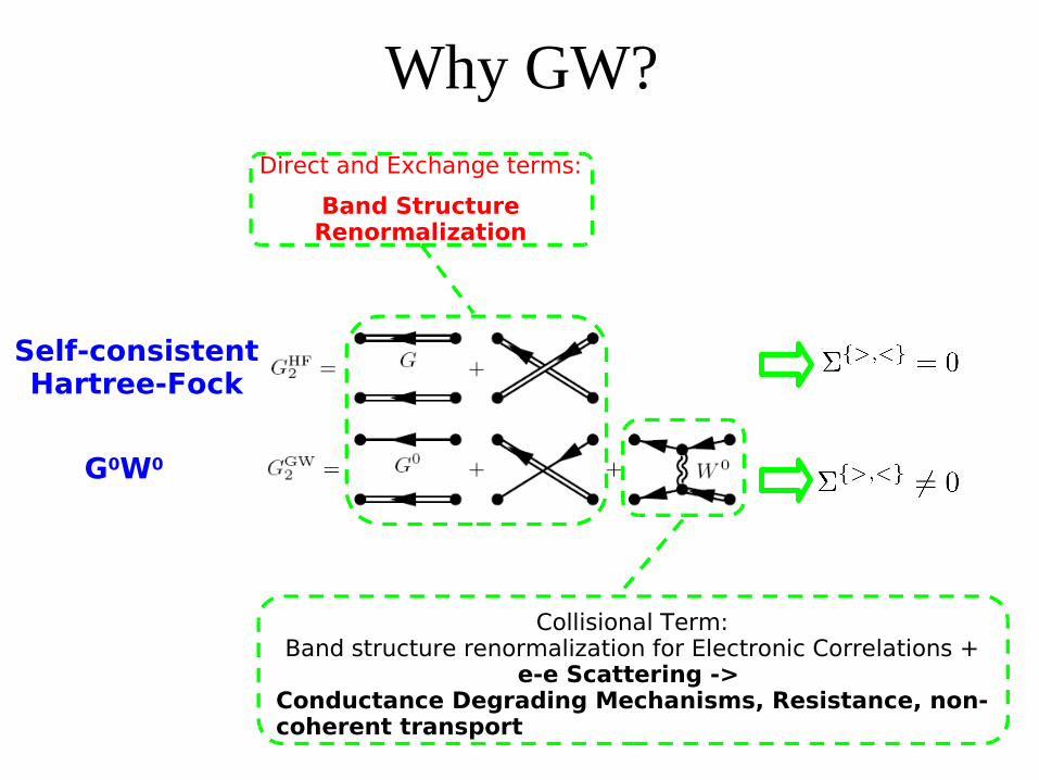
Why GW?Direct and Exchange terms:

Band Structure Renormalization

Collisional Term:Band structure renormalization for Electronic Correlations +

e-e Scattering -> Conductance Degrading Mechanisms, Resistance, non-coherent transport

G0W0

Self-consistent Hartree-Fock

Why GW?

Band renormalization (band gap) in good agreement with the experiment!

NEGF Quantum Transportresolution scheme

So far applied to model Hamiltonians (Anderson, Kondo) But very few applications for real systems

Iterating the Kinetic Equations(G and Σ have to be recalculated at each iteration):

Highly Time-consuming

Our Scheme• Approximations:

1) G0W0 Non Self-Consistently

2) Equilibrium (linear response, small bias)

3) Neglect Transient (Steady-State)

• We take into account:1) Many-Body Correlations (Renormalization of the

electronic structure)

2) e-e Scattering (appearance of Resistance and Loss-of-Coherence)

3) Finite Lifetime and Dynamical effects (beyond Plasmon-Pole GW)

Flow diagram

DFT

MLWFs GW

Real space Ham.

Transport

http://www.abinit.org

http://www.wannier-transport.orghttp://www.wannier.org

Results onAu Monoatomic Chain

GW on Au Monoatomic chain: renormalization of the energies

GW Au chainKohn-Sham Au chain

Monoatomic Gold chain:GW vs DFT bandplot

P. Darancet, A. Ferretti, D. Mayou, et V. Olevano, PRB 75, 075102 (2007).

PPM Plasmon-Pole ModelAC Analytic ContinuationCD Contour Deformation(more or less the same)

GW vs DFTLandauer Conductance

• non-negligible rearrangement of the conductance channels• Still ballistic conductor (flat plateaus)

e-e scattering switched on only in the Central part

CL R

Self-Energy and Spectral Function

• The Analytic Continuation smooths the more accurate Contour Deformation

e-e scattering only in the Conductor

Broadening of the peaks:➔ QP lifetime

Loss of Conductance:➔ Appearance of Resistance

e-e scattering in conductor and leads

➔No contact resistance (small increase in the central part)➔Appearance of Satellite Conductance Channels

sate

ll ite

C / V characteristics: GW vs EXP

e-e

e-ph

}EXPERIMENT

P. Darancet, A. Ferretti, D. Mayou, and V. Olevano, PRB 75, 075102 (2007).

N. Agrait , PRL 88, 216803 (2002) Frederiksen et al., PRL 93, 256601 (2004)

Results on Molecular Junctions

BDA and BDT

• Benzene Dithiol/Diamine @ Au(111) are among the most studied systems.

BDA BDT

Experiment vs DFT on BDA

BDA

No mol.

Break Au junctions:L. Venkataraman et al., Nano Letters 6, 458 (2006)

zero-bias conductance [G0]

EXP 0.007DFT 0.018

DFT overestimate of the conductance!

Is it due to e-e many-body effects?

G = 0.007

First essays: 1PM-IC model

• The , simplified to a HOMO-LUMO shissor operator, are adjusted on the experiment or on another model: the Image-Charge (IC) model

1PM=∑mm∣m

mol ⟩ ⟨mmol∣

m

Neaton et al. PRL 97, 216405 (2006)Quek et al. Nano Letters 7, 3472 (2007)Mowbray et al. JCP 128, 11103 (2008)

• The self-energy is modeled by a simple one-projector (on molecular orbitals) model (1PM):

1PM vs DFT vs Experiment

• The 1PM model reduces the conductance

zero-bias conductance [G0]

DFT 0.018EXP 0.0071PM 0.004

Our GW calculation on BDA@gold

• Cost of 1 iteration in BDA:~ 250 bands 250 x 250 matrix elements→

96 irreducible k-points, 11463 plane waves

~ 1 month on 32 processors.

• Approximations:✗ neglect of the non-hermitian component

real quasiparticles, no lifetimes→

✗ neglect of the dynamic behavior

• Fully accounted:✔non diagonal elements

Ab Initio GW conductance

• Ab initio GW reduces the conductance

• GW is still half-way →further SC iterations?

• 1PM is beyond

zero-bias conductance [G0]

DFT 0.018GW 0.013EXP 0.0071PM 0.004

Conductance reduction mechanism

LDOS difference: GW - DFT

Eigenchannel difference: GW - 1PM

Important changes both on the leads and on the molecule

Important differences between the 1PM model and the ab initio GW

→ the 1PM model reduces the conductance but does not reproduce the correct physics. Red: + Blue: -

3PM model3PM=∑m

mmol∣m

mol ⟩ ⟨mmol∣∑l

lAu−sp∣l

Au−sp ⟩ ⟨lAu−sp∣∑l

lAu−d∣l

Au−d ⟩ ⟨lAu−d∣

BDA BDT-H BDT-h BDT-p

DFT 0.018 0.034 0.28 0.37

GW 0.013 In progress

3PM 0.011 0.010 0.25 0.36

1PM 0.004 In progress NA NA

EXP 0.007 0.010

3PM model:

• More physical

• Promising results

BDA BDT

Conclusions

• GW e-e correlations in quantum transport:– Static real part of self-energy (GW-LB)

➔ modification of the conductance profile.➔ reduction of the 0-bias conductance

– Non-hermitean part of the self-energy (NEGF-GW)➔ loss-of-coherence, dissipative effects.

– Full dynamical self-energy (NEGF-GW)➔ appearance of satellites

• GW in good agreement with the Experiment both on:

– the smooth drop in the Au-chain conductance

– the absolute 0-bias conductance in BDA@gold

GW instead then KS leads