Abaqus/Dymola Co-Simulation:

cantilever beam

Author: Ahmed ELLEUCH Angelo PALMIERI

1

Sources: Digital Product Simulation

2

Co-Simulation

Introduction Co-Simulation■ The Abaqus co-simulation technique can be used to solve complex systems that

include electronics such as control systems, electro-mechanics, hydraulics, and

pneumatics by coupling Abaqus with Dymola, a general-purpose logical modeling

software distributed by Dassault Systèmes.

■ A logical-physical model looks as follows:

The communication between the two solvers is described schematically as shown below:

3

Abaqus physical

Model

Dymola logicalModel

Sensors

Actuators

Real Input

Real output

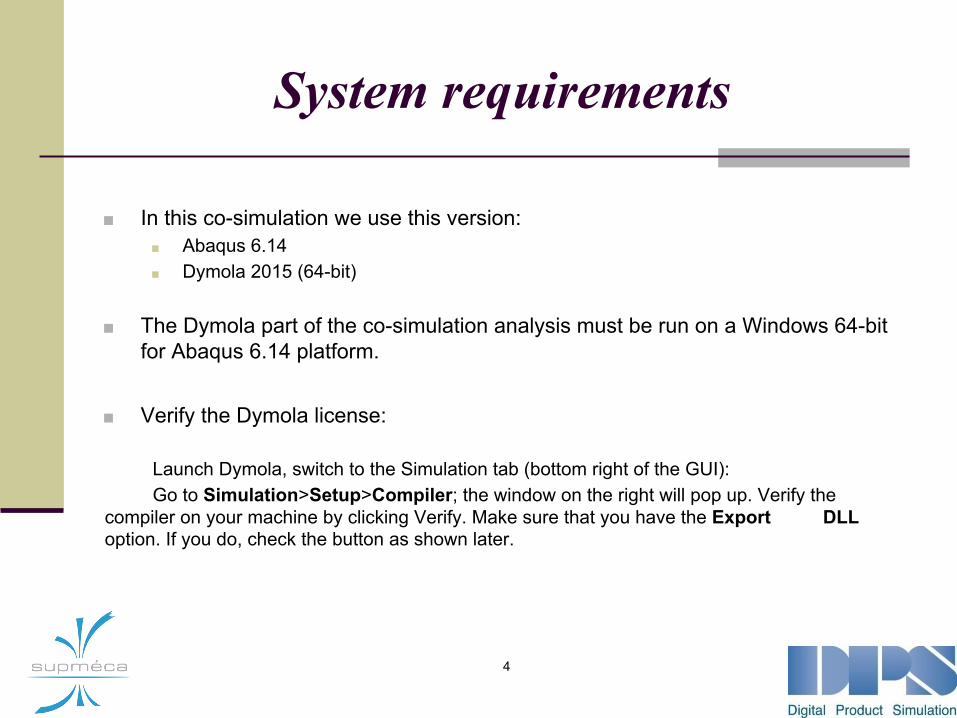
System requirements

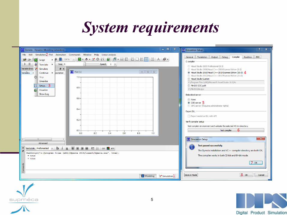
■ In this co-simulation we use this version:■ Abaqus 6.14■ Dymola 2015 (64-bit)

■ The Dymola part of the co-simulation analysis must be run on a Windows 64-bit for Abaqus 6.14 platform.

■ Verify the Dymola license:

Launch Dymola, switch to the Simulation tab (bottom right of the GUI):Go to Simulation>Setup>Compiler; the window on the right will pop up. Verify the

compiler on your machine by clicking Verify. Make sure that you have the Export DLL option. If you do, check the button as shown later.

4

System requirements

5

Co-simulation objectives

■ Couple Dymola 2015 and Abaqus 6.14.

■ Develop a logical-physical modeling.

■ Create a simple control system in Dymola for co-simulation.

■ Run a co-simulation between Abaqus 6.14 and Dymola 2015.

■ Review the co-simulation results.

6

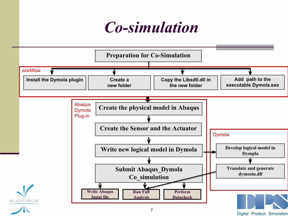
Co-simulation

7

Preparation for Co-Simulation

Install the Dymola plugin Create a new folder

Copy the Libsdll.dll in the new folder

Add path to the executable Dymola.exe

Create the physical model in Abaqus

Create the Sensor and the Actuator

Write new logical model in Dymola

Translate and generatedymosin.dll

workflow

Develop logical model in Dympla

Submit Abaqus_Dymola Co_simulation

Dymola

Abaqus Dymola Plug-in

Write Abaqus Input file

Run Full Analysis

Perform Datacheck

Co-simulation

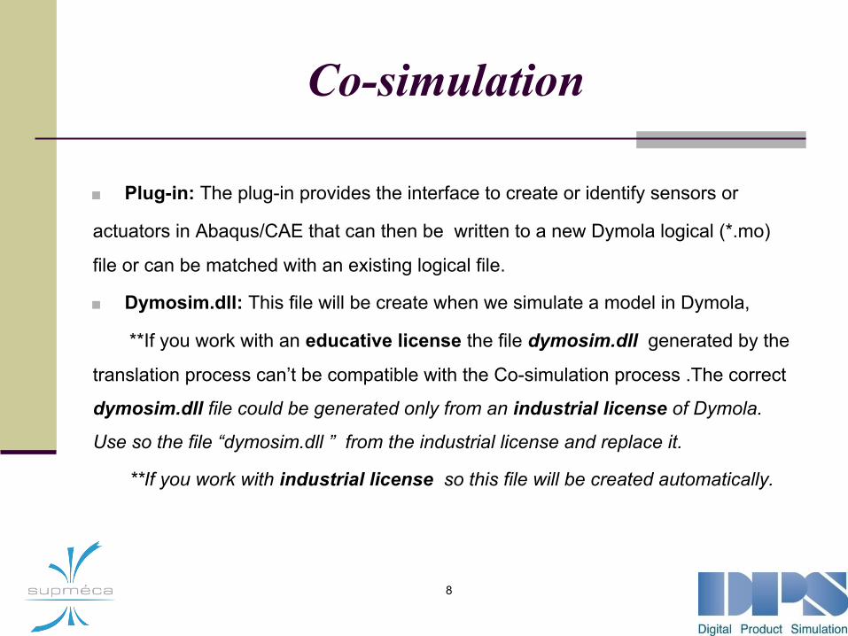
■ Plug-in: The plug-in provides the interface to create or identify sensors or

actuators in Abaqus/CAE that can then be written to a new Dymola logical (*.mo)

file or can be matched with an existing logical file.

■ Dymosim.dll: This file will be create when we simulate a model in Dymola,

**If you work with an educative license the file dymosim.dll generated by the

translation process can’t be compatible with the Co-simulation process .The correct

dymosim.dll file could be generated only from an industrial license of Dymola.

Use so the file “dymosim.dll ” from the industrial license and replace it.

**If you work with industrial license so this file will be created automatically.

8

Co-simulation: examples

9

Scheme of Co-simulation for a Beam:

In this Scheme we will make a sensor on the beam that sends the position to Dymola and receive an amplitude pressure (Actuator) to reach some points in function of the time.

Co-simulation: examples

10

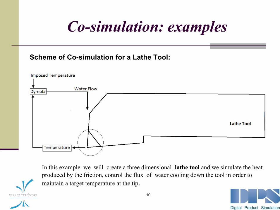
Scheme of Co-simulation for a Lathe Tool:

In this example we will create a three dimensional lathe tool and we simulate the heat produced by the friction, control the flux of water cooling down the tool in order to maintain a target temperature at the tip.

11

Preparation for Co-Simulation

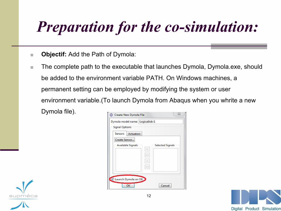
Preparation for the co-simulation: ■ Objectif: Add the Path of Dymola:

■ The complete path to the executable that launches Dymola, Dymola.exe, should

be added to the environment variable PATH. On Windows machines, a

permanent setting can be employed by modifying the system or user

environment variable.(To launch Dymola from Abaqus when you whrite a new

Dymola file).

12

Preparation for the co-simulation: 1- From the Control Panel\System and Security\System, click on the Advanced

tab and then click Environment Variables.

2- Click New and enter PATH for the variable name and specify the path to the

Dymola executable (“C:\Program Files (x86)\Dymola 2015\bin64”) for the variable

value. If there is an existing PATH variable, edit the variable and add the path to the

executable to the variable value.

3- Click OK and OK.

13

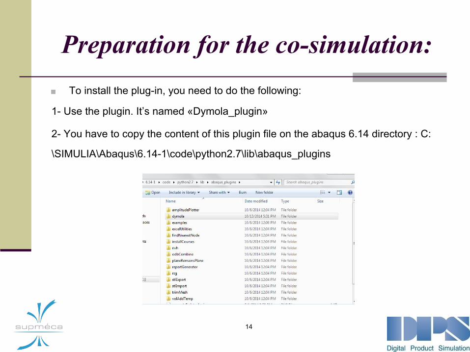
Preparation for the co-simulation: ■ To install the plug-in, you need to do the following:

1- Use the plugin. It’s named «Dymola_plugin»

2- You have to copy the content of this plugin file on the abaqus 6.14 directory : C:

\SIMULIA\Abaqus\6.14-1\code\python2.7\lib\abaqus_plugins

14

Preparation for the co-simulation: 2- Then you can open the Abaqus 6.14 and verify if the plugin is installed by going to

JOB section and see under the “plugins” toolbox if there is the Dymola plugin.

15

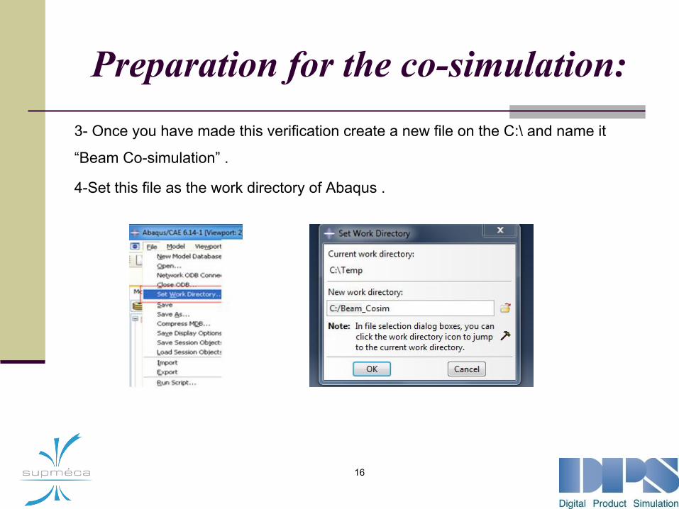
Preparation for the co-simulation: 3- Once you have made this verification create a new file on the C:\ and name it

“Beam Co-simulation” .

4-Set this file as the work directory of Abaqus .

16

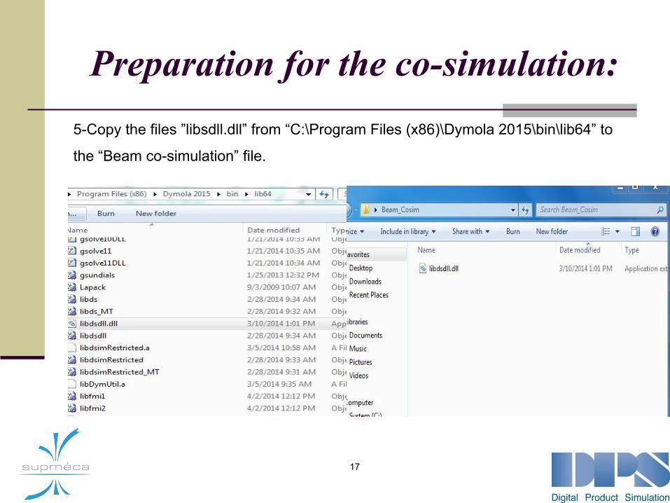
Preparation for the co-simulation: 5-Copy the files ”libsdll.dll” from “C:\Program Files (x86)\Dymola 2015\bin\lib64” to

the “Beam co-simulation” file.

17

Preparation for the co-simulation: -The complete path to the executable that launches Dymola, Dymola.exe, should be added to the environment

■ If there is an existing PATH variable, edit the variable and add the path to the executable to the variable value” C:\Program Files (x86)\Dymola 2015\bin64’’

18

Creation of the Abaqus model

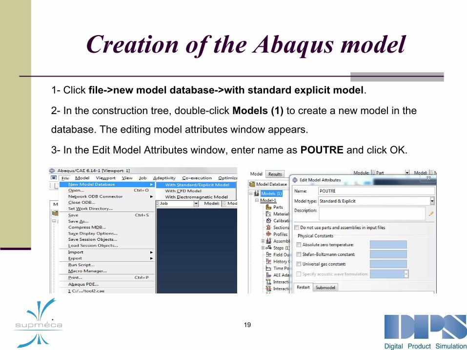
Creation of the Abaqus model 1- Click file->new model database->with standard explicit model.

2- In the construction tree, double-click Models (1) to create a new model in the

database. The editing model attributes window appears.

3- In the Edit Model Attributes window, enter name as POUTRE and click OK.

. 19

Creation of the Abaqus model 4- Select poutre as "root" (right click at POUTRE and select Set as Root menu that appears). The tree is then built as shown in Figure.

5- Save the database, select File → Save at the main menu and select “Beam co-simulation” as the database.Click OK. The .cae is added automatically in the Beam Co-simulation file.

**In this section, you will create a deformable solid 3D drawing of the beam profile in 2D (a rectangle) and then extruding.

1- In the construction tree, double-click Parts to create a newshare in the beam model. Create the Share window appears.

20

Creation of the Abaqus model 2- In this window, enter the name as POUTRE and specify an approximate size of 600 Accept the default settings. 3D Deformable Solid, Extrude. Click Continue.

21

Creation of the Abaqus model Draw the rectangular profile:

1- Click the Create tool Lines: Rectangle appears in the upper right of the toolbar.

2- Use the Add Dimension to define the dimensions of the top and left sides of

the rectangle.

The upper side must have a horizontal

dimension of 200 mm and the left side

must have a vertical dimension of 20 mm.

22

Creation of the Abaqus model 3- Click Done or the middle mouse button. Depth of the extrusion 25 in the Edit Base Extrusion window, then click OK.

23

Creation of the Abaqus model **Create a linear elastic material with a Young's modulus of 210 000 MPa and

Poisson's ratio of 0.3

1- In the construction tree, double-click Materials to create a new material.

2- Edit Material window will open, name the material: Steel.

3- Starting material menu, select Mechanical → Elasticity → Elastic.

4- Select General → Density and enter a density of 7.8 E9 tonnes/mm3. Click OK

24

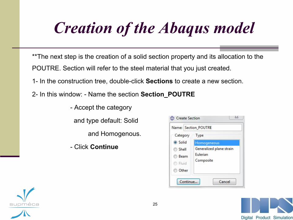
Creation of the Abaqus model **The next step is the creation of a solid section property and its allocation to the

POUTRE. Section will refer to the steel material that you just created.

1- In the construction tree, double-click Sections to create a new section.

2- In this window: - Name the section Section_POUTRE

- Accept the category

and type default: Solid

and Homogenous.

- Click Continue

25

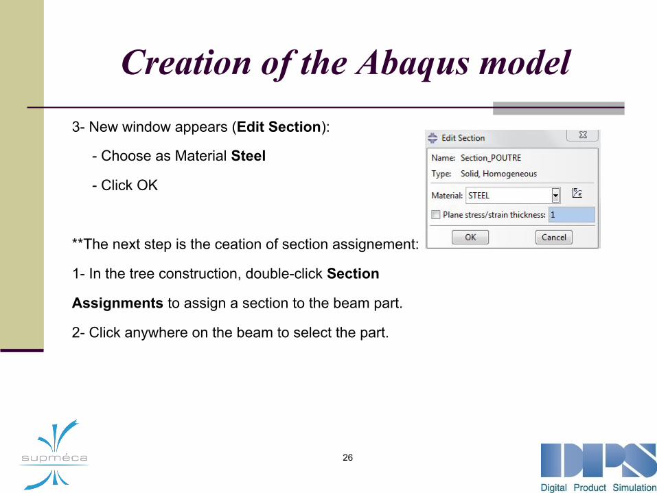
Creation of the Abaqus model 3- New window appears (Edit Section):

- Choose as Material Steel

- Click OK

**The next step is the ceation of section assignement:

1- In the tree construction, double-click Section

Assignments to assign a section to the beam part.

2- Click anywhere on the beam to select the part.

26

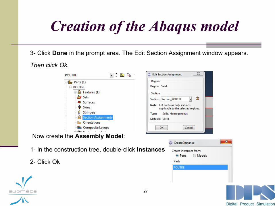
Creation of the Abaqus model 3- Click Done in the prompt area. The Edit Section Assignment window appears.

Then click Ok.

Now create the Assembly Model:

1- In the construction tree, double-click Instances

2- Click Ok

27

Creation of the Abaqus model **After the creation of the Assembly Model, we create step

1- Double-click Steps, new window appear

2- In this window: - Name the step POUTRE LOADED. - From the list of available procedures in the Create Step window, select Static, General. - Click Continue.

28

Creation of the Abaqus model

**The editing step window appears:

1- At the Description field on the Basic tab, enter Charge poutre.

2- Set a value of 0.1 as an initial increment size.

29

Creation of the Abaqus model **CREATE THE APPLICATION OF BOUNDARY CONDITIONS TO AN END OF

THE BEAM:

1- In the construction tree, double-click BCs to create a new boundary condition.

2- In this window:

- Name the boundary condition Fixed.

- Choose the step POUTRE LOADED in which the boundary condition will be

activated.

- At the Category list, accept the default choice: Mechanical.

- Click Continue.

30

Creation of the Abaqus model 3- Select the face you want and click OK.

4- The Edit Boundary Condition window appears. Choose ENCASTRED to block

all degrees of freedom and then click OK.

31

Creation of the Abaqus model **The next step is: APPLYING PRESSURE ON THE UPPER SURFACE OF THE

BEAM

1- Double-click the Loads container to create a new load

2- In this window:

- Name the load PRESSURE.

- Select Beam loaded as the load step at which will be

applied.

- For the Category list, accept the default choice: Mechanical.

- At the Types for Selected Step list, select Pressure.

- Click Continue.

32

Creation of the Abaqus model 3- In the graphics window, select the top face as the face which the load is Applied.

4- In the Edit Load window:

- Enter a magnitude of 0.002 for loading

- Accept the default selections for options and Amplitude Distribution.

- Click OK

33

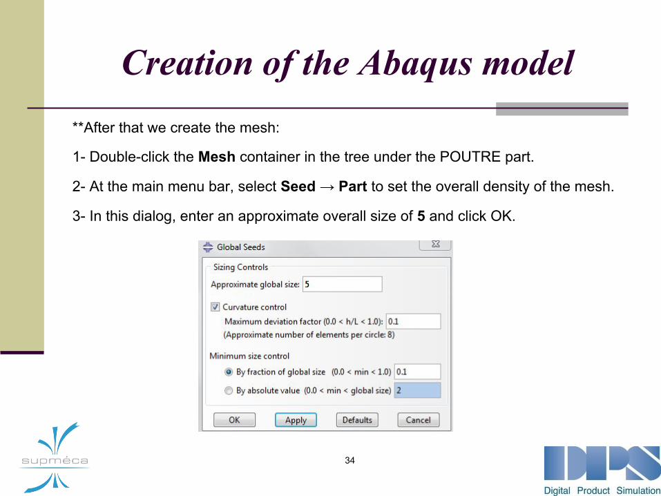
Creation of the Abaqus model **After that we create the mesh:

1- Double-click the Mesh container in the tree under the POUTRE part.

2- At the main menu bar, select Seed → Part to set the overall density of the mesh.

3- In this dialog, enter an approximate overall size of 5 and click OK.

34

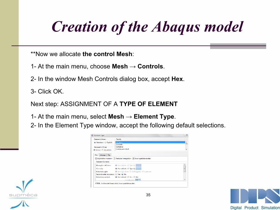
Creation of the Abaqus model **Now we allocate the control Mesh:

1- At the main menu, choose Mesh → Controls.

2- In the window Mesh Controls dialog box, accept Hex.

3- Click OK.

Next step: ASSIGNMENT OF A TYPE OF ELEMENT

1- At the main menu, select Mesh → Element Type. 2- In the Element Type window, accept the following default selections.

35

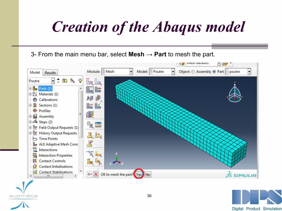
Creation of the Abaqus model 3- From the main menu bar, select Mesh → Part to mesh the part.

4- Click Yes in the prompt box.

36

37

Preparing the Dymola model

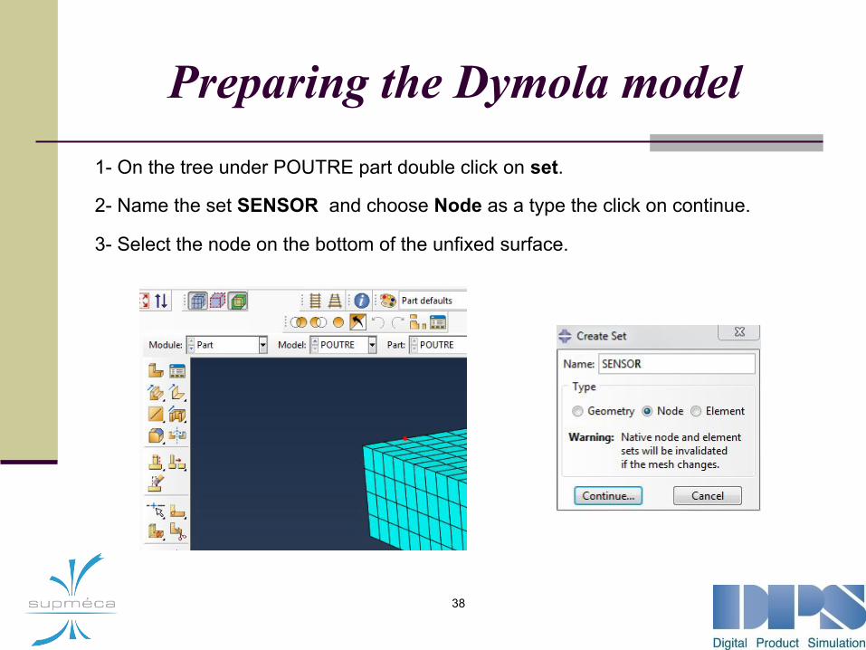
Preparing the Dymola model1- On the tree under POUTRE part double click on set.

2- Name the set SENSOR and choose Node as a type the click on continue.

3- Select the node on the bottom of the unfixed surface.

38

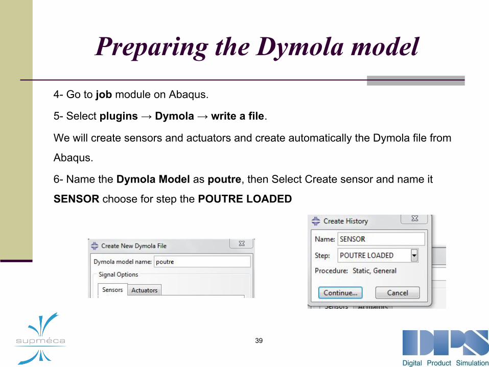
Preparing the Dymola model4- Go to job module on Abaqus.

5- Select plugins → Dymola → write a file.

We will create sensors and actuators and create automatically the Dymola file from

Abaqus.

6- Name the Dymola Model as poutre, then Select Create sensor and name it

SENSOR choose for step the POUTRE LOADED

39

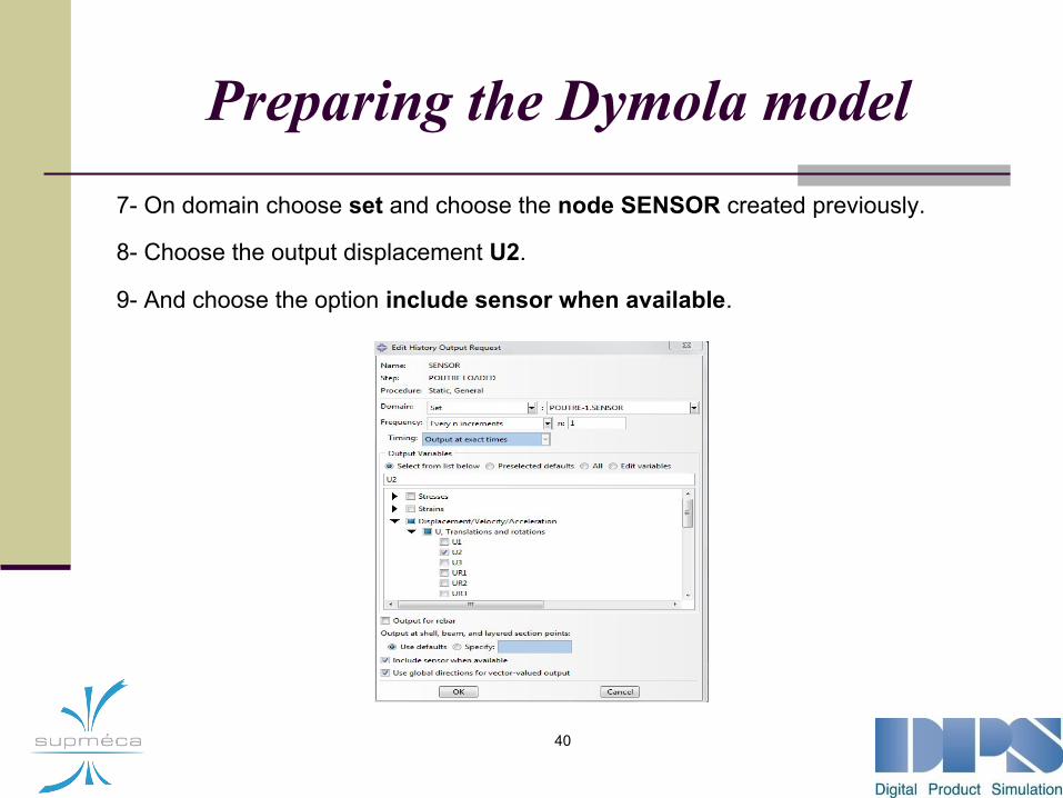
Preparing the Dymola model7- On domain choose set and choose the node SENSOR created previously.

8- Choose the output displacement U2.

9- And choose the option include sensor when available.

40

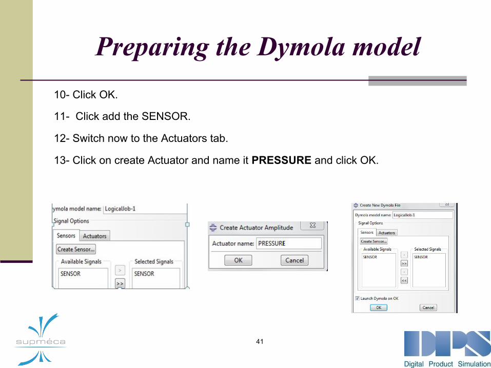
Preparing the Dymola model10- Click OK.

11- Click add the SENSOR.

12- Switch now to the Actuators tab.

13- Click on create Actuator and name it PRESSURE and click OK.

41

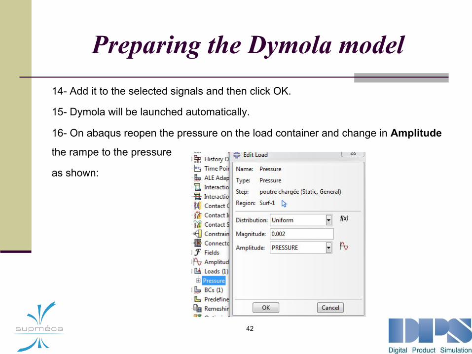
Preparing the Dymola model14- Add it to the selected signals and then click OK.

15- Dymola will be launched automatically.

16- On abaqus reopen the pressure on the load container and change in Amplitude

the rampe to the pressure

as shown:

42

43

SETUP DYMOLA

SETUP DYMOLA

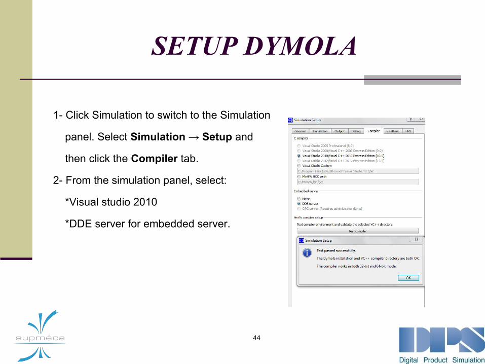
1- Click Simulation to switch to the Simulation

panel. Select Simulation → Setup and

then click the Compiler tab.

2- From the simulation panel, select:

*Visual studio 2010

*DDE server for embedded server.

44

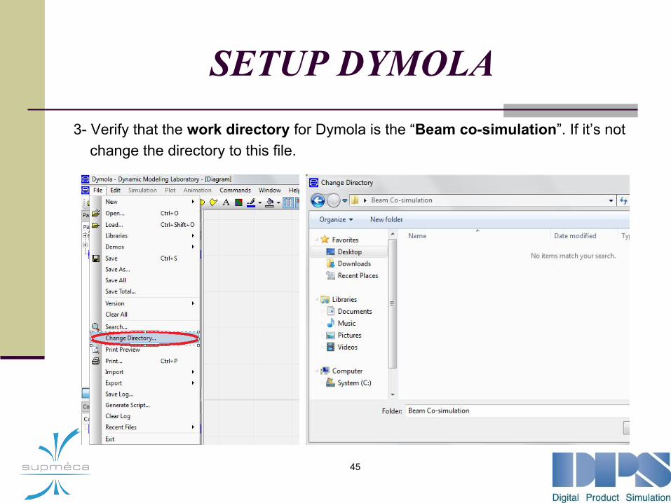
SETUP DYMOLA 3- Verify that the work directory for Dymola is the “Beam co-simulation”. If it’s not change the directory to this file.

45

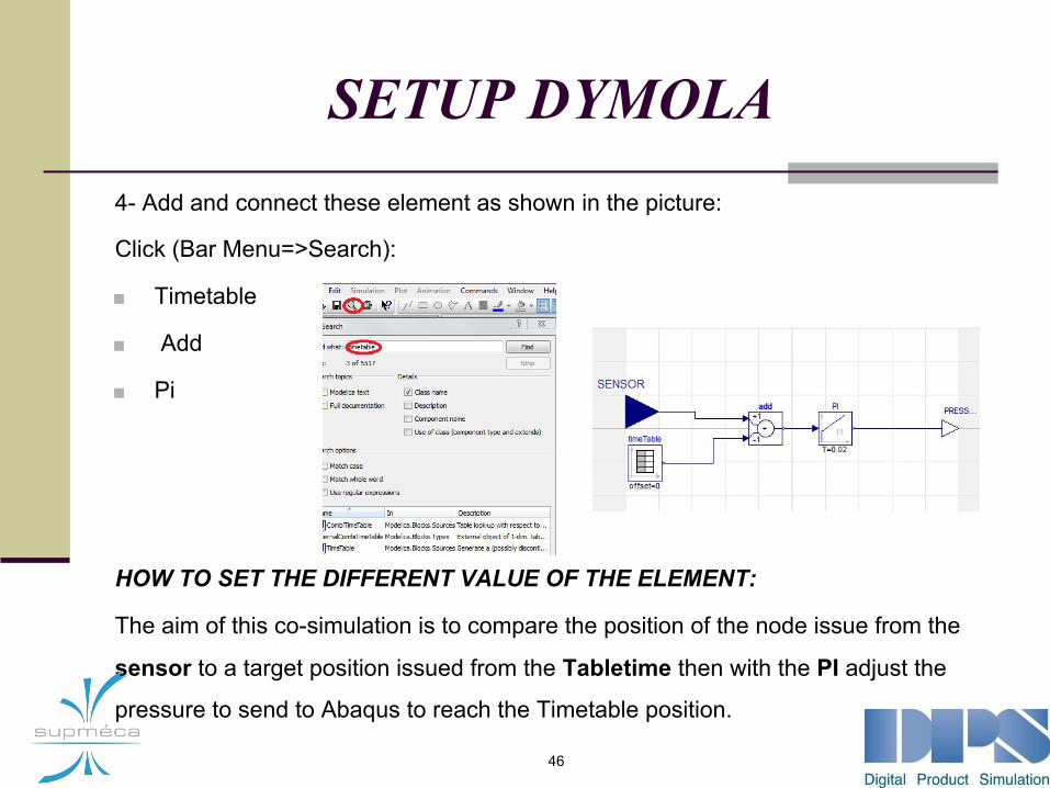
SETUP DYMOLA4- Add and connect these element as shown in the picture:

Click (Bar Menu=>Search):

■ Timetable

■ Add

■ Pi

HOW TO SET THE DIFFERENT VALUE OF THE ELEMENT:

The aim of this co-simulation is to compare the position of the node issue from the

sensor to a target position issued from the Tabletime then with the PI adjust the

pressure to send to Abaqus to reach the Timetable position.

46

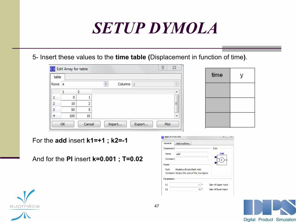
SETUP DYMOLA5- Insert these values to the time table (Displacement in function of time).

For the add insert k1=+1 ; k2=-1

And for the PI insert k=0.001 ; T=0.02

47

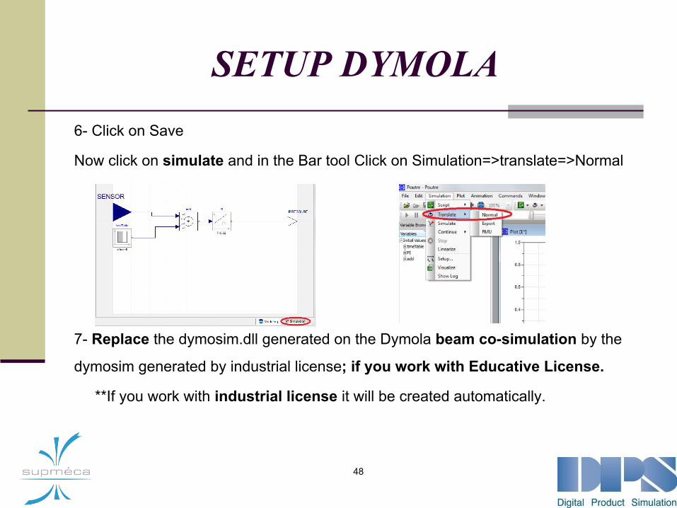
SETUP DYMOLA6- Click on Save

Now click on simulate and in the Bar tool Click on Simulation=>translate=>Normal

7- Replace the dymosim.dll generated on the Dymola beam co-simulation by the

dymosim generated by industrial license; if you work with Educative License.

**If you work with industrial license it will be created automatically.

48

49

Launching the co-simulation

Launching the co-simulationOn abaqus:

1- Select JOB.

2- Select:Plugins → Dymola → Submit a Co-simulation.

3- In dymola file name click on select and search for the “Poutre.mo” dymola file

on the beam co-simulation directory.

4- Choose for the step: POUTRE LOADED.

5- Choose variable for Time stepping scheme.

6- Then click Submit to start the co-simulation.

7- Click Monitor and refresh.

50

Launching the co-simulation

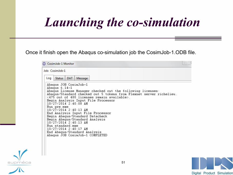
Once it finish open the Abaqus co-simulation job the CosimJob-1.ODB file.

51

Launching the co-simulation

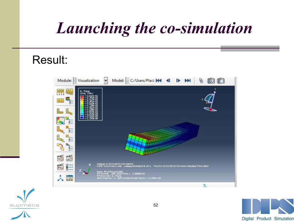
Result:

52

Launching the co-simulationIn the menu bar click Result → History Output.Chose Spatial displacement U2 and click Plot.

53

54

Cosimulation: Graphical method

(with beam file already done)

Cosimulation: Graphical method

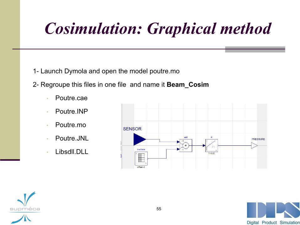
1- Launch Dymola and open the model poutre.mo

2- Regroupe this files in one file and name it Beam_Cosim

• Poutre.cae

• Poutre.INP

• Poutre.mo

• Poutre.JNL

• Libsdll.DLL

55

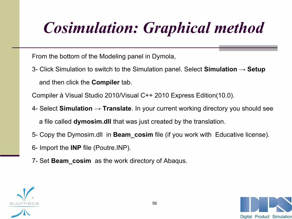
Cosimulation: Graphical methodFrom the bottom of the Modeling panel in Dymola,

3- Click Simulation to switch to the Simulation panel. Select Simulation → Setup

and then click the Compiler tab.

Compiler à Visual Studio 2010/Visual C++ 2010 Express Edition(10.0).

4- Select Simulation → Translate. In your current working directory you should see

a file called dymosim.dll that was just created by the translation.

5- Copy the Dymosim.dll in Beam_cosim file (if you work with Educative license).

6- Import the INP file (Poutre.INP).

7- Set Beam_cosim as the work directory of Abaqus.

. 56

Cosimulation: Graphical method

57

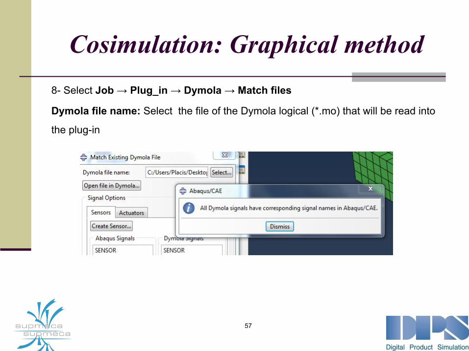
8- Select Job → Plug_in → Dymola → Match files

Dymola file name: Select the file of the Dymola logical (*.mo) that will be read into

the plug-in

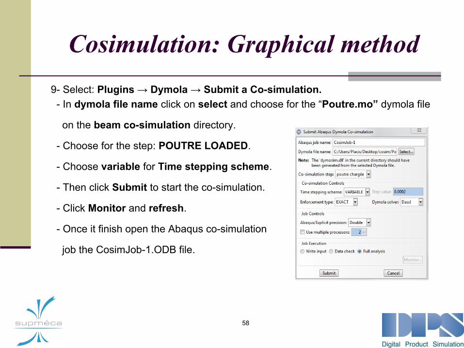
Cosimulation: Graphical method9- Select: Plugins → Dymola → Submit a Co-simulation. - In dymola file name click on select and choose for the “Poutre.mo” dymola file

on the beam co-simulation directory.

- Choose for the step: POUTRE LOADED.

- Choose variable for Time stepping scheme.

- Then click Submit to start the co-simulation.

- Click Monitor and refresh.

- Once it finish open the Abaqus co-simulation

job the CosimJob-1.ODB file.

58

Cosimulation: Graphical method■ Once it finish open the Abaqus co-simulation job the CosimJob-1.ODB file

59

Method of Lines: Heat equation

■ MOL solution to the heat equation

Picture from „Scientific Computing“, M. Heath