54
ABC The method: practical overview
| Date post: | 03-Jan-2016 |
| Category: |
Documents |
| Upload: | rosalyn-singleton |
| View: | 221 times |
| Download: | 6 times |
ABC
The method: practical overview
1. Applications of ABC in population genetics2. Motivation for the application of ABC3. ABC approach
1. Characteristics of an ABC methodology2. Algorithm of an ABC inference3. Limitations of the ABC approach4. Typical ABC run
4. Present work1. Compare the ABC algorithm with MCMC2. Study the use of different summary statistics3. Study the use of ABC in more complex scenario4. “State of art” of the software
5. Future developments
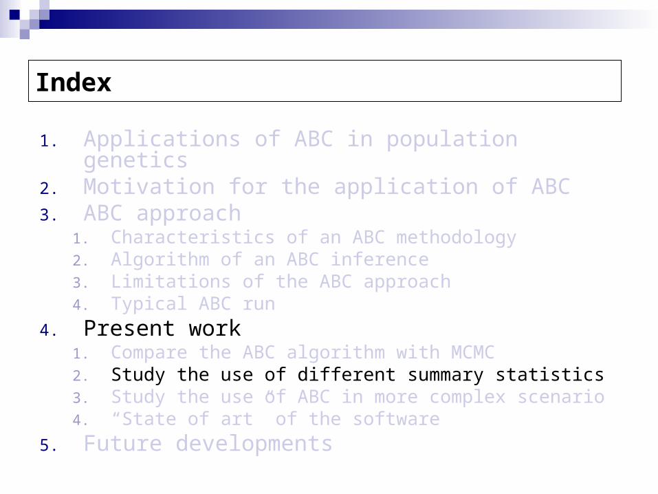
Index
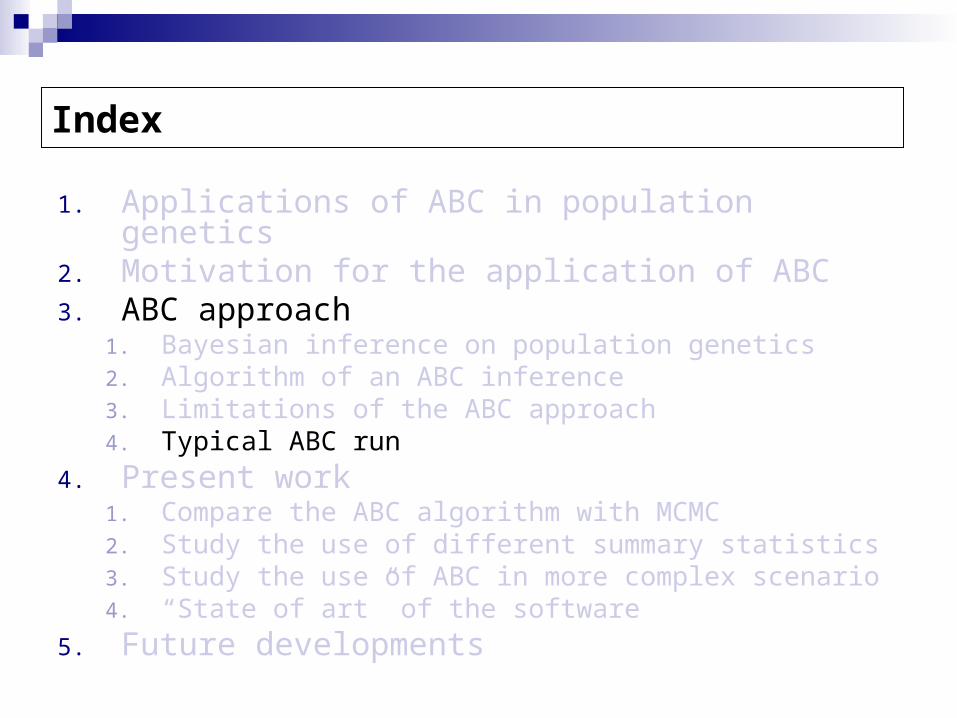
1. Applications of ABC in population genetics2. Motivation for the application of ABC3. ABC approach
1. Characteristics of an ABC methodology2. Algorithm of an ABC inference3. Limitations of the ABC approach4. Typical ABC run
4. Present work1. Compare the ABC algorithm with MCMC2. Study the use of different summary statistics3. Study the use of ABC in more complex scenario4. “State of art” of the software
5. Future developments
Index
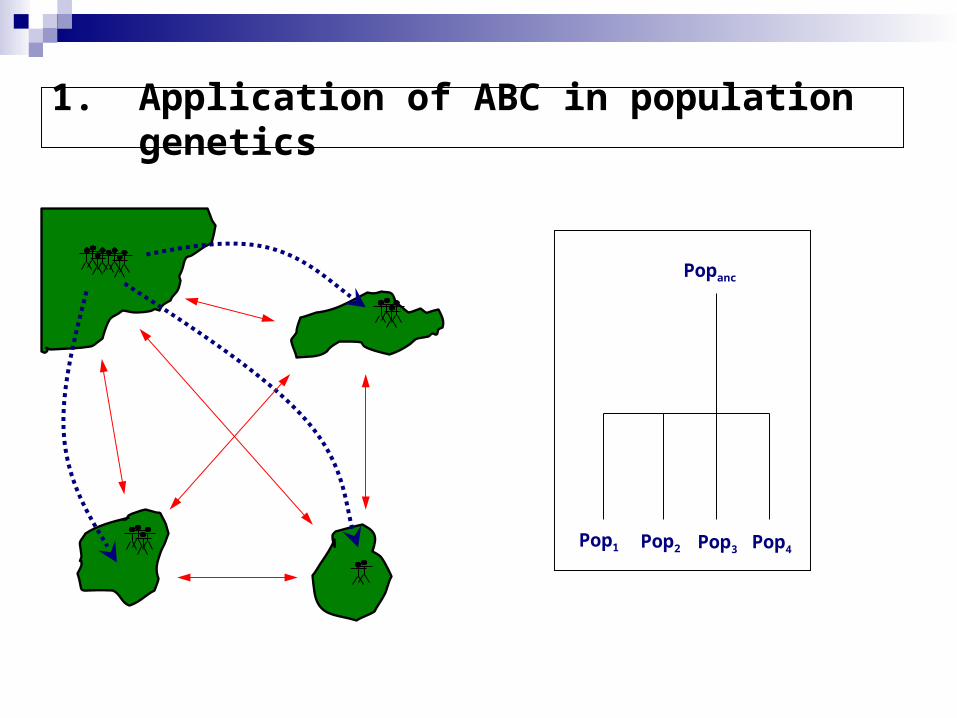
1. Application of ABC in population genetics
Popanc
Pop3 Pop4Pop2Pop1
1. Applications of ABC in population genetics2. Motivation for the application of ABC3. ABC approach
1. Characteristics of an ABC methodology2. Algorithm of an ABC inference3. Limitations of the ABC approach4. Typical ABC run
4. Present work1. Compare the ABC algorithm with MCMC2. Study the use of different summary statistics3. Study the use of ABC in more complex scenario4. “State of art” of the software
5. Future developments
Index
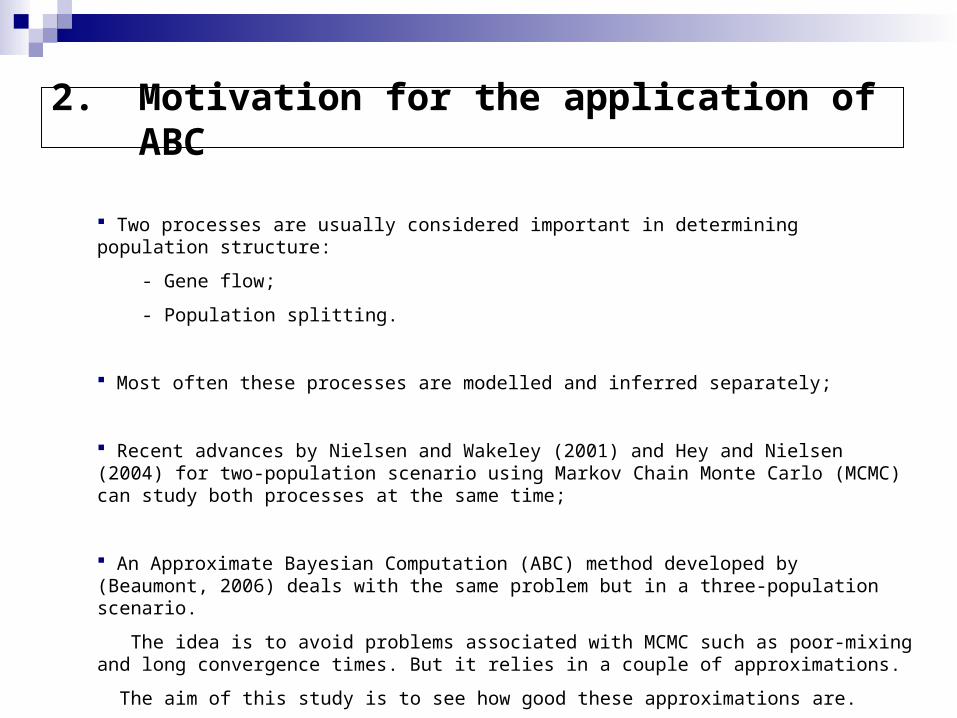
Two processes are usually considered important in determining population structure:
- Gene flow;
- Population splitting.
Most often these processes are modelled and inferred separately;
Recent advances by Nielsen and Wakeley (2001) and Hey and Nielsen (2004) for two-population scenario using Markov Chain Monte Carlo (MCMC) can study both processes at the same time;
An Approximate Bayesian Computation (ABC) method developed by (Beaumont, 2006) deals with the same problem but in a three-population scenario.
The idea is to avoid problems associated with MCMC such as poor-mixing and long convergence times. But it relies in a couple of approximations.
The aim of this study is to see how good these approximations are.
2. Motivation for the application of ABC
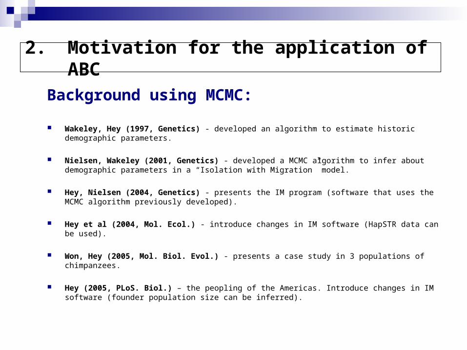
Wakeley, Hey (1997, Genetics) - developed an algorithm to estimate historic demographic parameters.
Nielsen, Wakeley (2001, Genetics) - developed a MCMC algorithm to infer about demographic parameters in a “Isolation with Migration” model.
Hey, Nielsen (2004, Genetics) - presents the IM program (software that uses the MCMC algorithm previously developed).
Hey et al (2004, Mol. Ecol.) - introduce changes in IM software (HapSTR data can be used).
Won, Hey (2005, Mol. Biol. Evol.) - presents a case study in 3 populations of chimpanzees.
Hey (2005, PLoS. Biol.) – the peopling of the Americas. Introduce changes in IM software (founder population size can be inferred).
Background using MCMC:
2. Motivation for the application of ABC
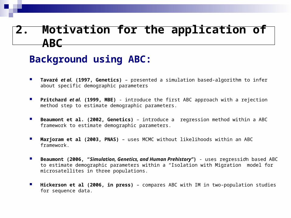
Background using ABC:
2. Motivation for the application of ABC
Tavaré et al. (1997, Genetics) – presented a simulation based-algorithm to infer about specific demographic parameters
Pritchard et al. (1999, MBE) - introduce the first ABC approach with a rejection method step to estimate demographic parameters.
Beaumont et al. (2002, Genetics) – introduce a regression method within a ABC framework to estimate demographic parameters.
Marjoram et al (2003, PNAS) – uses MCMC without likelihoods within an ABC framework.
Beaumont (2006, “Simulation, Genetics, and Human Prehistory”) - uses regression based ABC to estimate demographic parameters within a “Isolation with Migration” model for microsatellites in three populations.
Hickerson et al (2006, in press) – compares ABC with IM in two-population studies for sequence data.
1. Applications of ABC in population genetics2. Motivation for the application of ABC3. ABC approach
1. Characteristics of an ABC methodology2. Algorithm of an ABC inference3. Limitations of the ABC approach4. Typical ABC run
4. Present work1. Compare the ABC algorithm with MCMC2. Study the use of different summary statistics3. Study the use of ABC in more complex scenario4. “State of art” of the software
5. Future developments
Index
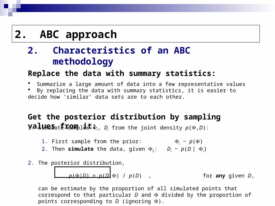
Replace the data with summary statistics:
2. ABC approach
2. Characteristics of an ABC methodology
Get the posterior distribution by sampling values from it:1. Simulate samples i, Di from the joint density p(,D):
1. First sample from the prior: i ~ p()
2. Then simulate the data, given i: Di ~ p(D | i)
2. The posterior distribution,
p(|D) = p(D,) / p(D) , for any given D,
can be estimate by the proportion of all simulated points that correspond to that particular D and divided by the proportion of points corresponding to D (ignoring ).
Summarize a large amount of data into a few representative values By replacing the data with summary statistics, it is easier to decide how ‘similar’ data sets are to each other.
1. Applications of ABC in population genetics2. Motivation for the application of ABC3. ABC approach
1. Bayesian inference on population genetics2. Characteristics of an ABC methodology3. Algorithm of an ABC inference4. Limitations of the ABC approach5. Typical ABC run
4. Present work1. Compare the ABC algorithm with MCMC2. Study the use of different summary statistics3. Study the use of ABC in more complex scenario4. “State of art” of the software
5. Future developments
Index
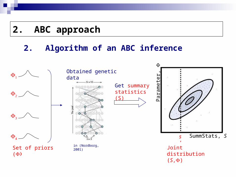
2. ABC approach
2. Algorithm of an ABC inference
SummStats, S
Par
amet
er,
Joint distribution (S,)Set of priors (
Get summary statistics (S)
Obtained genetic data
s’
in (Nordborg, 2001)
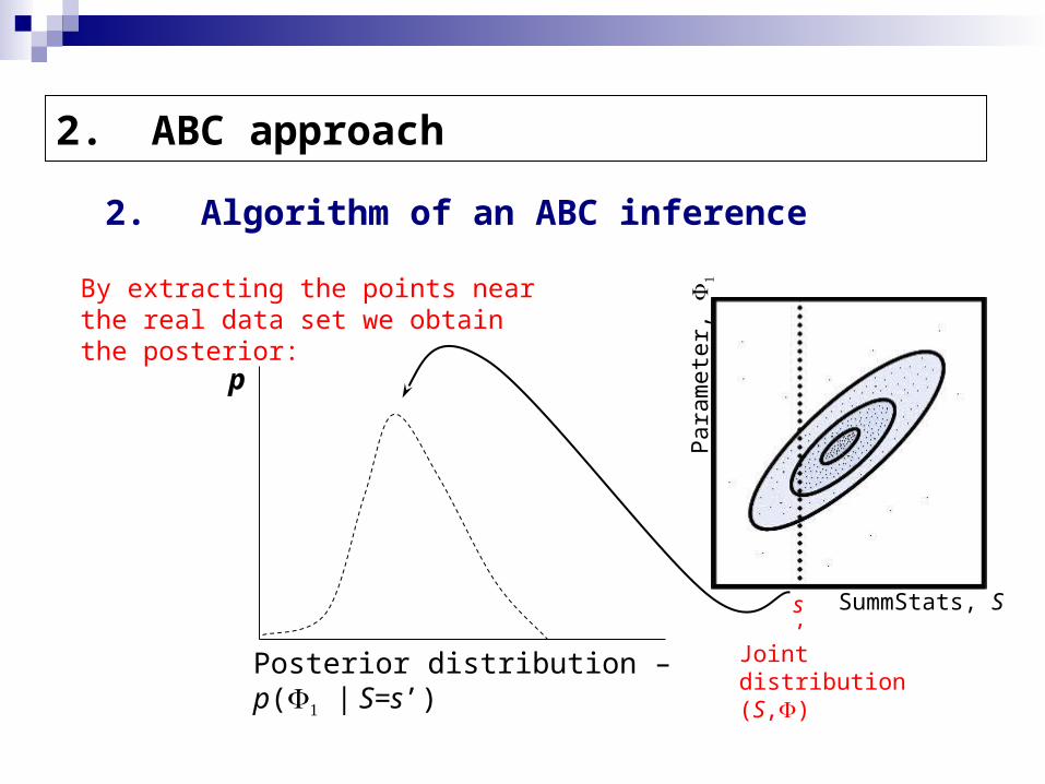
By extracting the points near the real data set we obtain the posterior:
2. Algorithm of an ABC inference
2. ABC approach
SummStats, S
Par
amet
er,
Joint distribution (S,)Posterior distribution – p( | S=s’)
p
s’
1. Applications of ABC in population genetics2. Motivation for the application of ABC3. ABC approach
1. Characteristics of an ABC methodology2. Algorithm of an ABC inference3. Limitations of the ABC approach4. Typical ABC run
4. Present work1. Compare the ABC algorithm with MCMC2. Study the use of different summary statistics3. Study the use of ABC in more complex scenario4. “State of art” of the software
5. Future developments
Index
2. ABC approach
Natural limitation due to lack of information in data sets
Limitation on the number of summary statistics used
Limitation on the calculation of summary statistic (time consuming)
Limitation on the time consumption of the simulation step
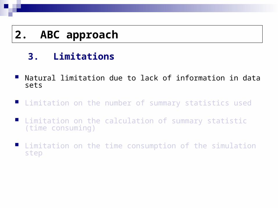
3. Limitations
2. ABC approach
Natural limitation due to lack of information in data sets
Limitation on the number of summary statistics used
Limitation on the calculation of summary statistic (time consuming)
Limitation on the time consumption of the simulation step
3. Limitations
3. ABC approach
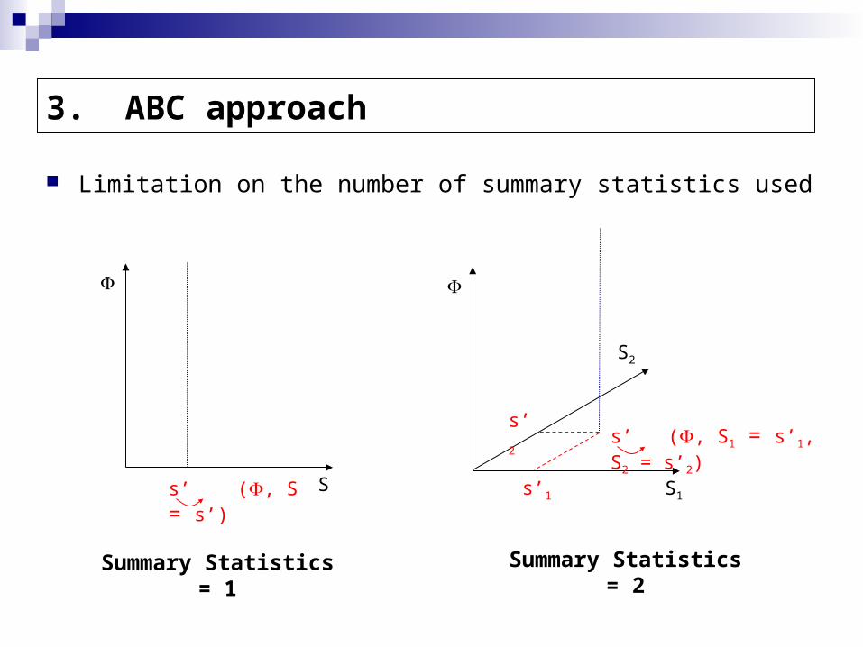
Limitation on the number of summary statistics used
Ss’ (, S = s’)
s’ (, S1 = s’1, S2 = s’2)s’2
s’1
S1
S2
Summary Statistics = 1 Summary Statistics = 2
2. ABC approach
Natural limitation due to lack of information in data sets
Limitation on the number of summary statistics used
Limitation on the calculation of summary statistic (time consuming)
Limitation on the time consumption of the simulation step
3. Limitations
1. Applications of ABC in population genetics2. Motivation for the application of ABC3. ABC approach
1. Bayesian inference on population genetics 2. Algorithm of an ABC inference3. Limitations of the ABC approach4. Typical ABC run
4. Present work1. Compare the ABC algorithm with MCMC2. Study the use of different summary statistics3. Study the use of ABC in more complex scenario4. “State of art” of the software
5. Future developments
Index
3. ABC approach
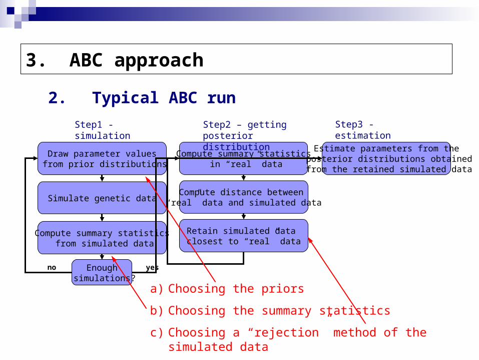
2. Typical ABC run
Draw parameter values from prior distributions
Simulate genetic data
Compute summary statistics from simulated data
Compute summary statistics in “real” data
Enough simulations?
Compute distance between “real” data and simulated data
Retain simulated data closest to “real” data
Estimate parameters from the posterior distributions obtained
from the retained simulated data
yesno
Step1 - simulation Step2 – getting posterior distribution
Step3 - estimation
a) Choosing the priors
b) Choosing the summary statistics
c) Choosing a “rejection” method of the simulated data
3. ABC approach
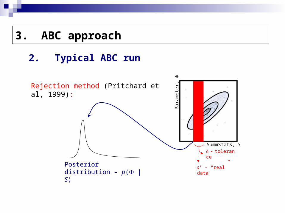
2. Typical ABC run
Rejection method (Pritchard et al, 1999):
SummStats, S
Par
amet
er,
tolerance
s’ – “real” dataPosterior distribution – p( | S)
3. ABC approach
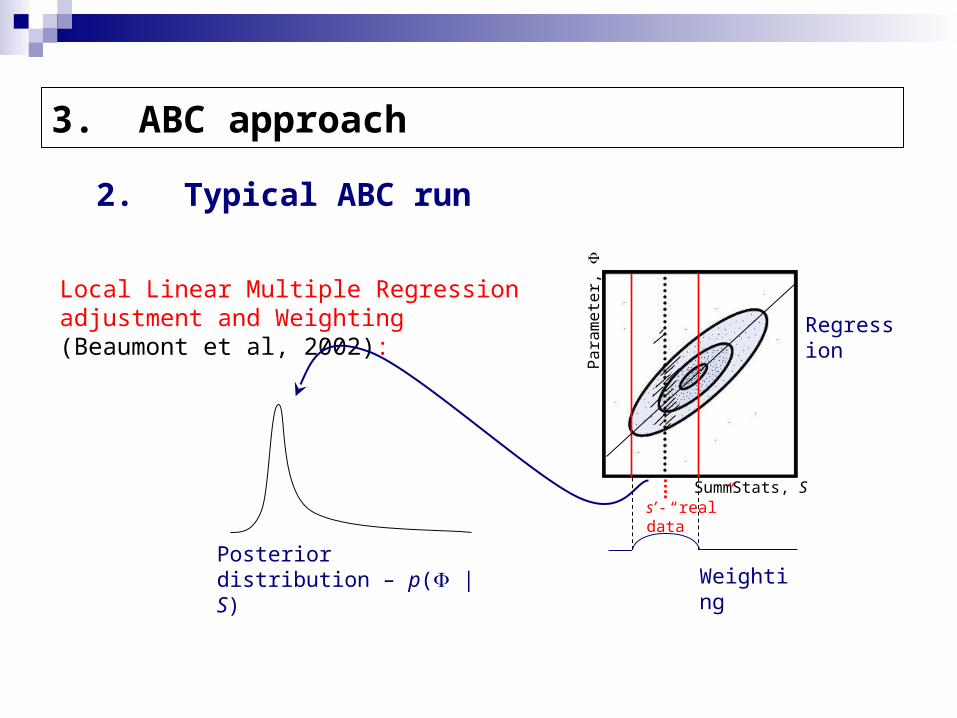
2. Typical ABC run
Local Linear Multiple Regression adjustment and Weighting (Beaumont et al, 2002):
SummStats, S
Par
amet
er,
s’ - “real” data
Posterior distribution – p( | S)Weighting
Regression
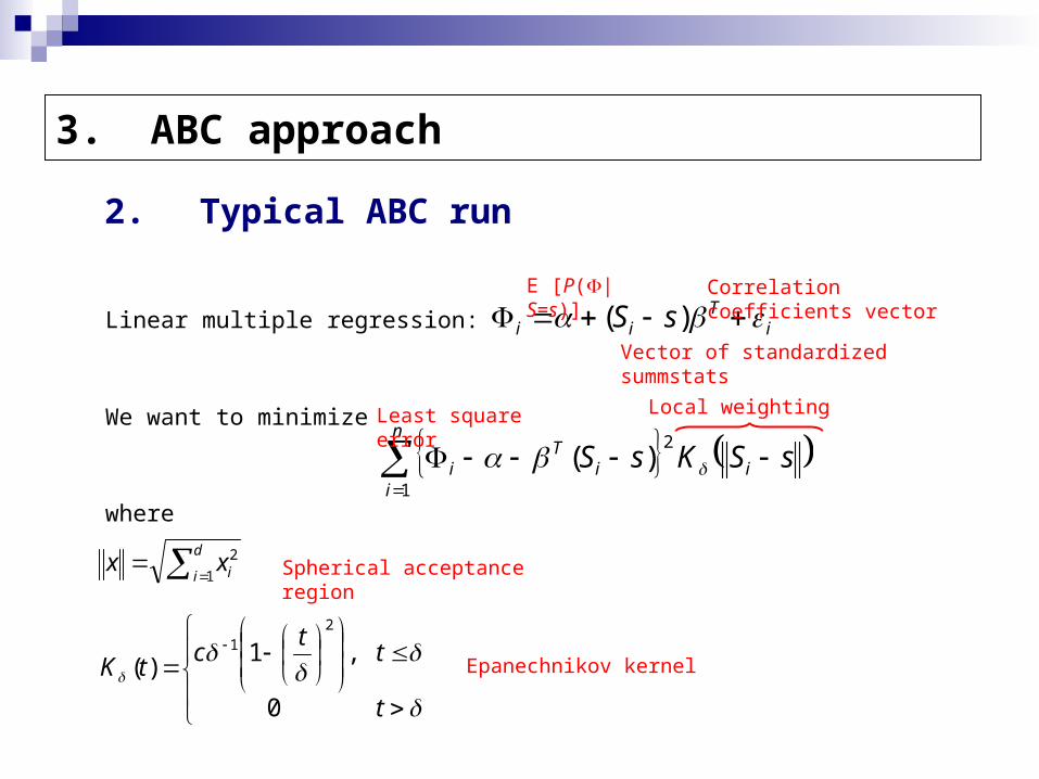
t
tt
ctK
0
,1)(
21
d
i ixx1
2
where
Epanechnikov kernel
n
iii
Ti sSKsS
1
2)(
We want to minimize
3. ABC approach
2. Typical ABC run
Spherical acceptance region
Local weighting
iT
ii sS )(Linear multiple regression:
Correlation coefficients vector
Vector of standardized summstats
E [P(|S=s)]
Least square error
* Tiii sS
3. ABC approach
2. Typical ABC run
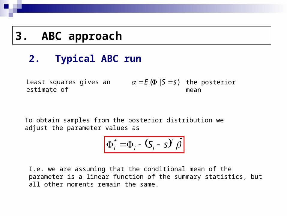
),|( sSE
To obtain samples from the posterior distribution we adjust the parameter values as
I.e. we are assuming that the conditional mean of the parameter is a linear function of the summary statistics, but all other moments remain the same.
Least squares gives an estimate of the posterior mean
1. Applications of ABC in population genetics2. Motivation for the application of ABC3. ABC approach
1. Characteristics of an ABC methodology2. Algorithm of an ABC inference3. Limitations of the ABC approach4. Typical ABC run
4. Present work1. Compare the ABC algorithm with MCMC 2. Study the use of different summary statistics3. Study the use of ABC in more complex scenario4. “State of art” of the software
5. Future developments
Index
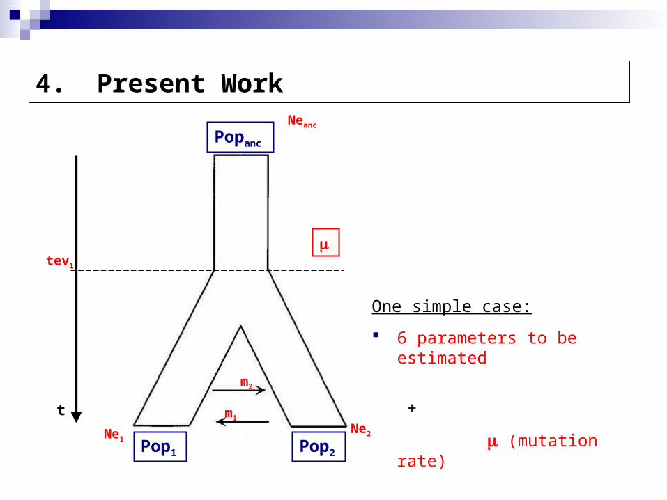
Popanc
Pop2Pop1
t
One simple case:
4. Present Work
m1
m2
Ne1Ne2
Neanc
tev1
6 parameters to be estimated
+
(mutation rate)
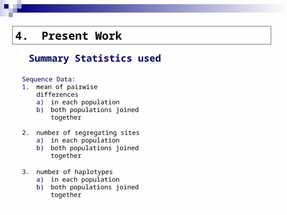
Summary Statistics used
Sequence Data:1. mean of pairwise differences
a) in each populationb) both populations joined together
2. number of segregating sitesa) in each populationb) both populations joined together
3. number of haplotypesa) in each populationb) both populations joined together
4. Present Work
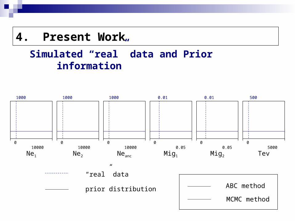
Simulated “real” data and Prior information
0 10000
1000 1000 1000 500
0 10000 0 10000 0 0.05 0 0.05 0 5000
0.01 0.01
Ne1 Ne2 Neanc TevMig2Mig1
“real” data
prior distribution ABC method
MCMC method
4. Present Work
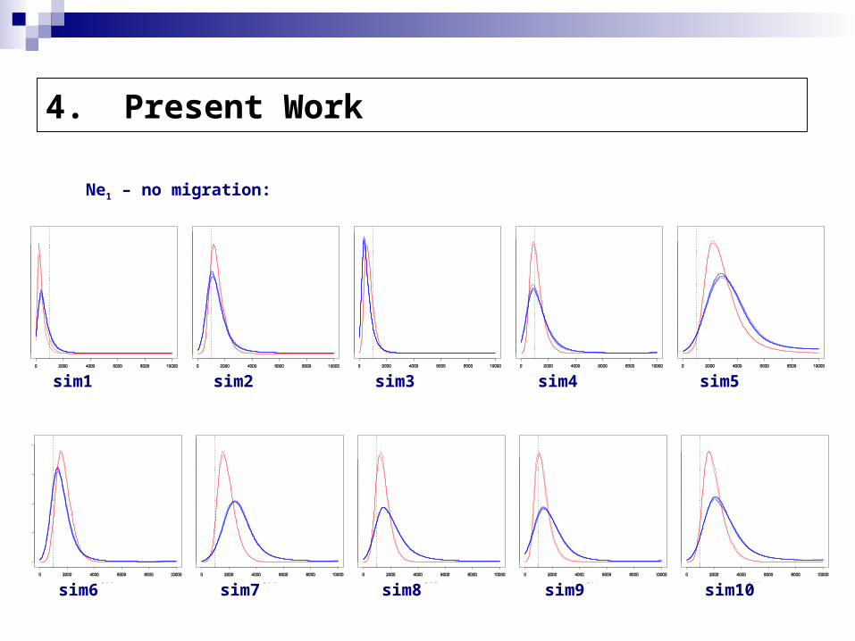
Ne1 – no migration:
sim1 sim3sim2 sim4 sim5
sim6 sim8sim7 sim9 sim10
4. Present Work
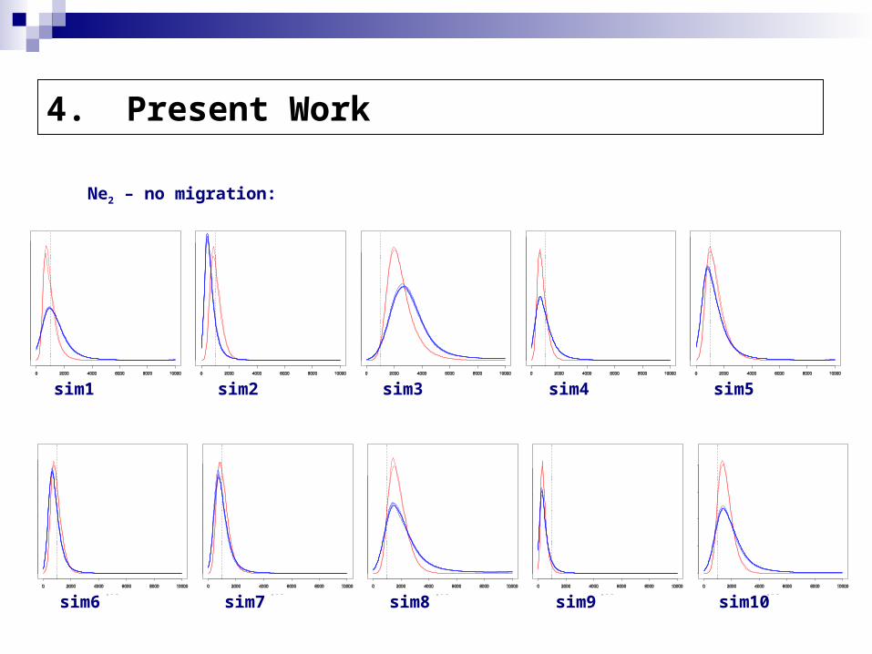
Ne2 – no migration:
sim1 sim3sim2 sim4 sim5
sim6 sim8sim7 sim9 sim10
4. Present Work
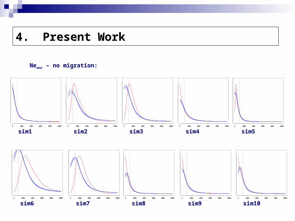
Neanc – no migration:
sim1 sim3sim2 sim4 sim5
sim6 sim8sim7 sim9 sim10
4. Present Work
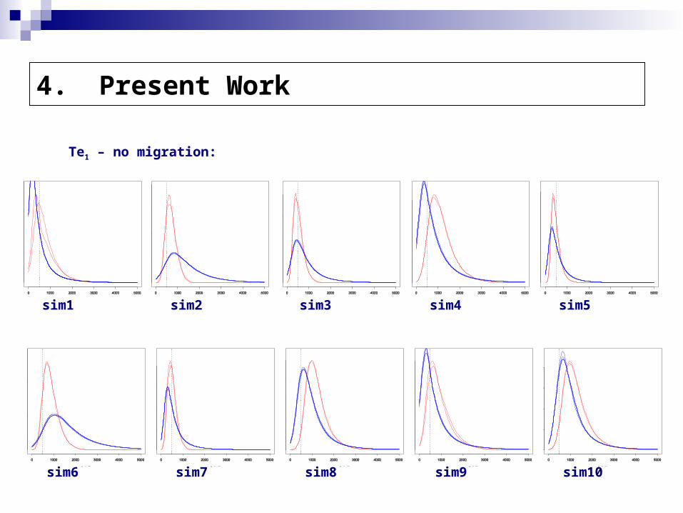
Te1 – no migration:
sim1 sim3sim2 sim4 sim5
sim6 sim8sim7 sim9 sim10
4. Present Work
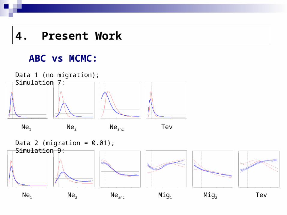
ABC vs MCMC:
Data 1 (no migration); Simulation 7:
Data 2 (migration = 0.01); Simulation 9:
Ne1 Ne2 Neanc Tev
Ne1 Ne2 Neanc TevMig2Mig1
4. Present Work
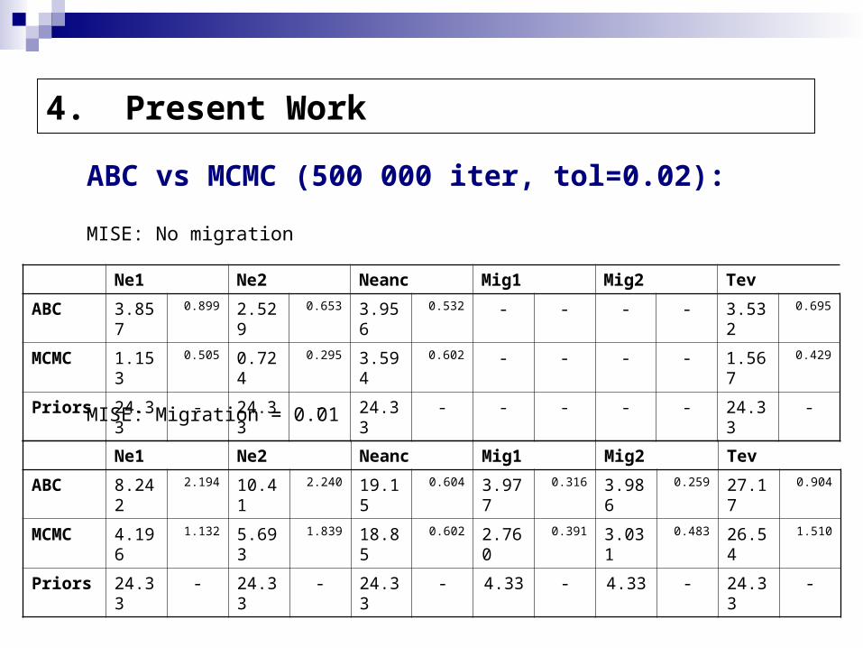
ABC vs MCMC (500 000 iter, tol=0.02):
Ne1 Ne2 Neanc Mig1 Mig2 Tev
ABC 3.857 0.899 2.529 0.653 3.956 0.532 - - - - 3.532 0.695
MCMC 1.153 0.505 0.724 0.295 3.594 0.602 - - - - 1.567 0.429
Priors 24.33 - 24.33 - 24.33 - - - - - 24.33 -
Ne1 Ne2 Neanc Mig1 Mig2 Tev
ABC 8.242 2.194 10.41 2.240 19.15 0.604 3.977 0.316 3.986 0.259 27.17 0.904
MCMC 4.196 1.132 5.693 1.839 18.85 0.602 2.760 0.391 3.031 0.483 26.54 1.510
Priors 24.33 - 24.33 - 24.33 - 4.33 - 4.33 - 24.33 -
MISE: No migration
MISE: Migration = 0.01
4. Present Work
1. Applications of ABC in population genetics2. Motivation for the application of ABC3. ABC approach
1. Characteristics of an ABC methodology2. Algorithm of an ABC inference3. Limitations of the ABC approach4. Typical ABC run
4. Present work1. Compare the ABC algorithm with MCMC2. Study the use of different summary statistics3. Study the use of ABC in more complex scenario4. “State of art” of the software
5. Future developments
Index
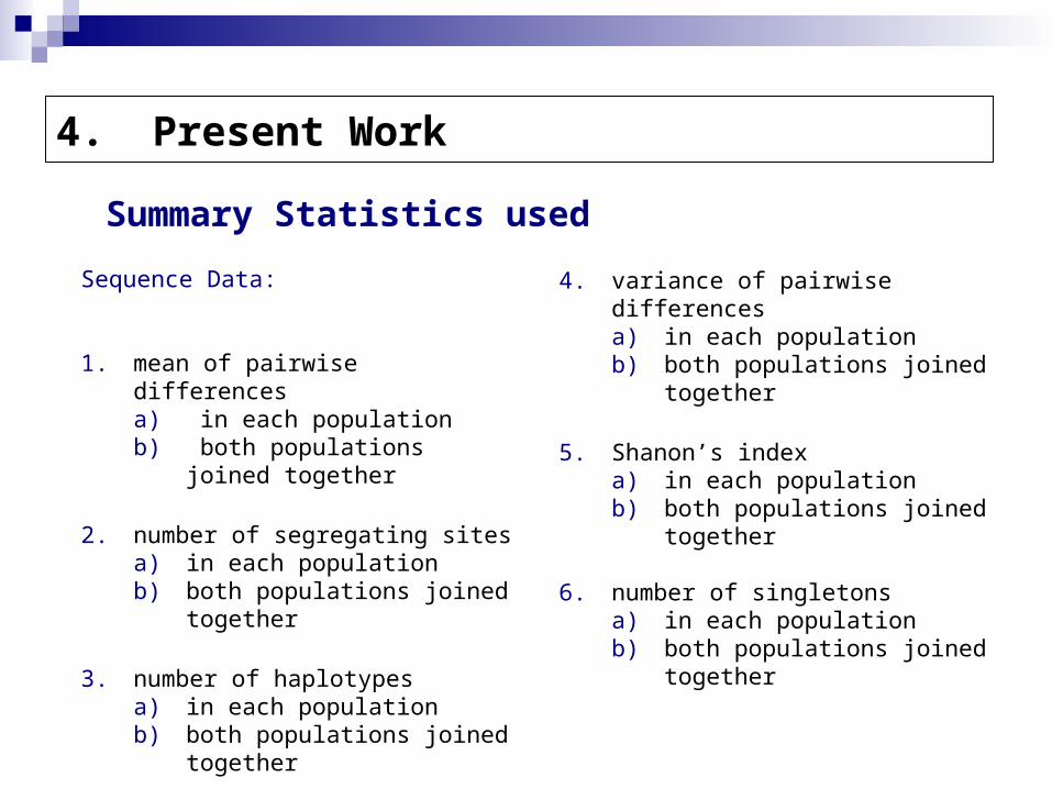
Summary Statistics used
Sequence Data:
1. mean of pairwise differencesa) in each populationb) both populations joined together
2. number of segregating sitesa) in each populationb) both populations joined together
3. number of haplotypesa) in each populationb) both populations joined together
4. variance of pairwise differencesa) in each populationb) both populations joined together
5. Shanon’s indexa) in each populationb) both populations joined together
6. number of singletonsa) in each populationb) both populations joined together
4. Present Work
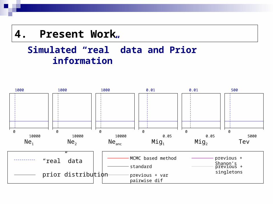
Simulated “real” data and Prior information
0 10000
1000 1000 1000 500
0 10000 0 10000 0 0.05 0 0.05 0 5000
0.01 0.01
Ne1 Ne2 Neanc TevMig2Mig1
“real” data
prior distribution
standard
previous + Shanon’s
previous + var pairwise dif
previous + singletons
MCMC based method
4. Present Work
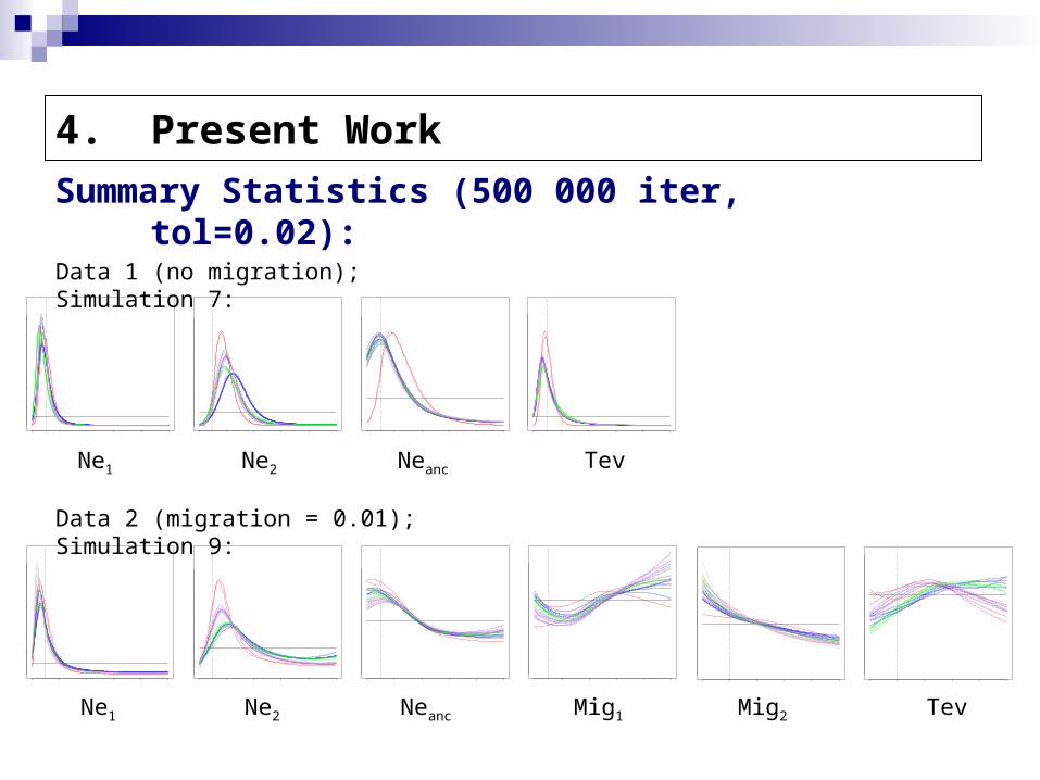
Summary Statistics (500 000 iter, tol=0.02):
Data 1 (no migration); Simulation 7:
Data 2 (migration = 0.01); Simulation 9:
Ne1 Ne2 Neanc Tev
Ne1 Ne2 Neanc TevMig2Mig1
4. Present Work
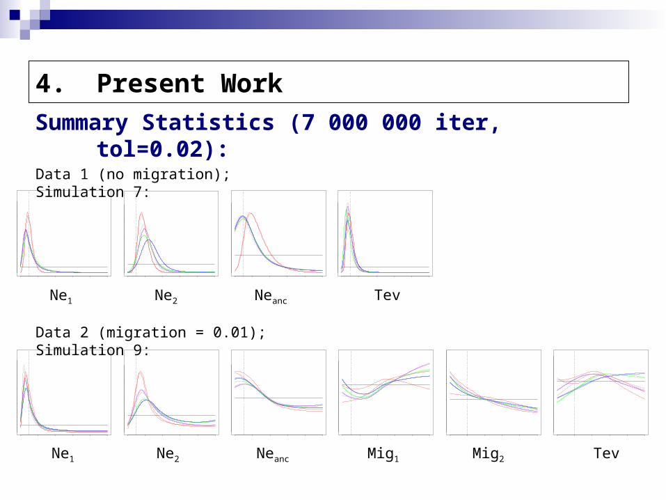
Summary Statistics (7 000 000 iter, tol=0.02):
Data 1 (no migration); Simulation 7:
Data 2 (migration = 0.01); Simulation 9:
Ne1 Ne2 Neanc Tev
Ne1 Ne2 Neanc TevMig2Mig1
4. Present Work
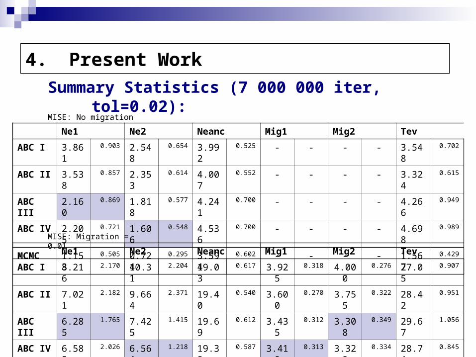
Summary Statistics (7 000 000 iter, tol=0.02):
Ne1 Ne2 Neanc Mig1 Mig2 Tev
ABC I 3.861 0.903 2.548 0.654 3.992 0.525 - - - - 3.548 0.702
ABC II 3.538 0.857 2.353 0.614 4.007 0.552 - - - - 3.324 0.615
ABC III 2.160 0.869 1.818 0.577 4.241 0.700 - - - - 4.266 0.949
ABC IV 2.205 0.721 1.606 0.548 4.536 0.700 - - - - 4.698 0.989
MCMC 1.153 0.505 0.724 0.295 3.594 0.602 - - - - 1.567 0.429
MISE: No migration
MISE: Migration = 0.01
Ne1 Ne2 Neanc Mig1 Mig2 Tev
ABC I 8.216 2.170 10.31 2.204 19.03 0.617 3.925 0.318 4.000 0.276 27.05 0.907
ABC II 7.021 2.182 9.664 2.371 19.40 0.540 3.600 0.270 3.755 0.322 28.42 0.951
ABC III 6.285 1.765 7.425 1.415 19.69 0.612 3.435 0.312 3.308 0.349 29.67 1.056
ABC IV 6.585 2.026 6.564 1.218 19.38 0.587 3.410 0.313 3.329 0.334 28.74 0.845
MCMC 4.196 1.132 5.693 1.839 18.85 0.602 2.760 0.391 3.031 0.483 26.54 1.510
4. Present Work
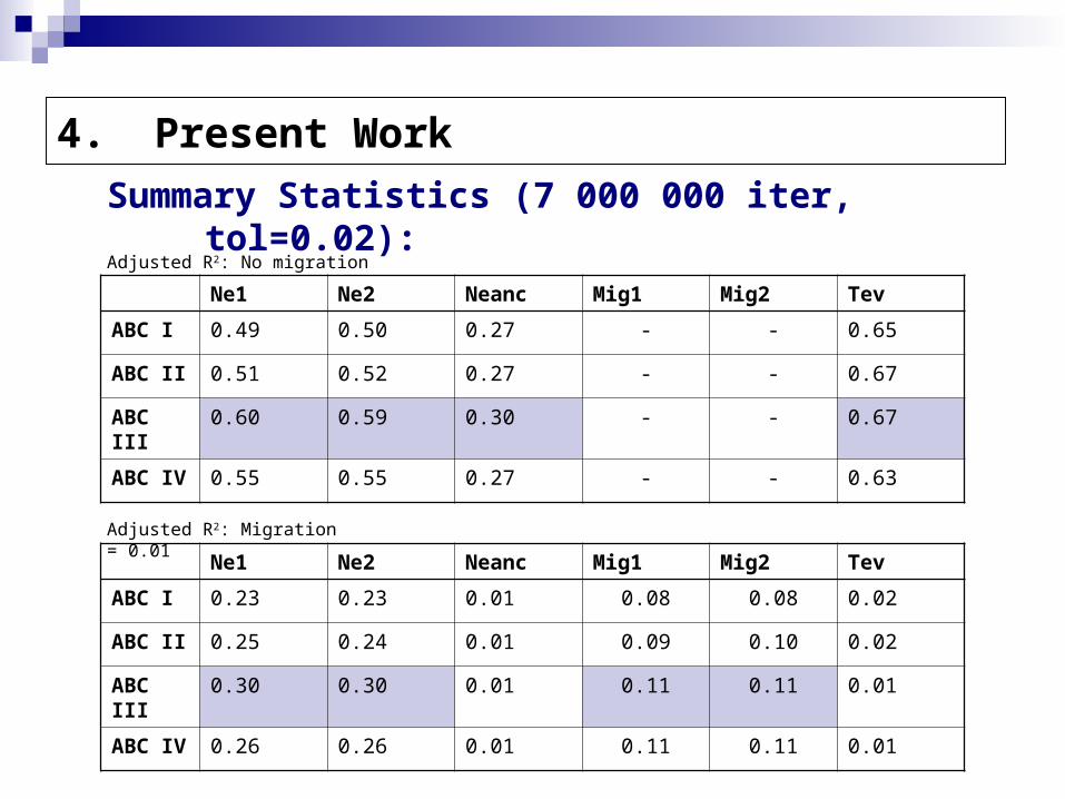
Summary Statistics (7 000 000 iter, tol=0.02):
Ne1 Ne2 Neanc Mig1 Mig2 Tev
ABC I 0.49 0.50 0.27 - - 0.65
ABC II 0.51 0.52 0.27 - - 0.67
ABC III 0.60 0.59 0.30 - - 0.67
ABC IV 0.55 0.55 0.27 - - 0.63
Adjusted R2: No migration
Adjusted R2: Migration = 0.01
Ne1 Ne2 Neanc Mig1 Mig2 Tev
ABC I 0.23 0.23 0.01 0.08 0.08 0.02
ABC II 0.25 0.24 0.01 0.09 0.10 0.02
ABC III 0.30 0.30 0.01 0.11 0.11 0.01
ABC IV 0.26 0.26 0.01 0.11 0.11 0.01
4. Present Work
1. Applications of ABC in population genetics2. Motivation for the application of ABC3. ABC approach
1. Characteristics of an ABC methodology2. Algorithm of an ABC inference3. Limitations of the ABC approach4. Typical ABC run
4. Present work1. Compare the ABC algorithm with MCMC2. Study the use of different summary statistics3. Study the use of ABC in more complex scenario4. “State of art” of the software
5. Future developments
Index
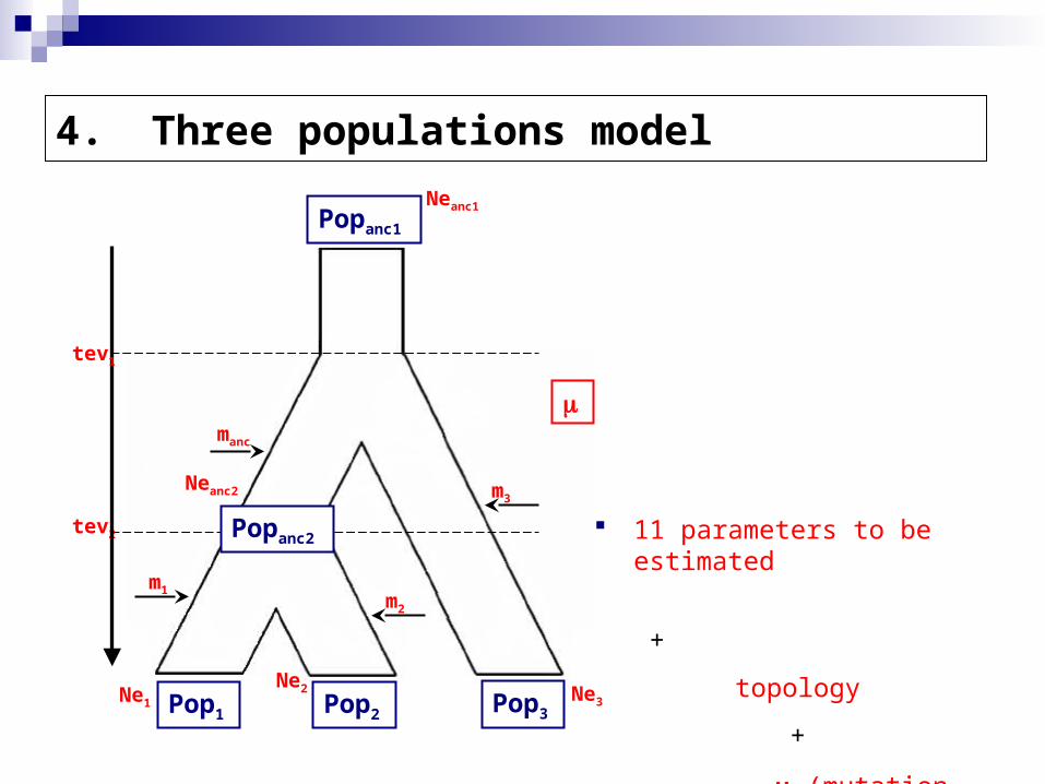
4. Three populations model
m1m2
Ne1 Ne3
Neanc1
tev2
11 parameters to be estimated
+
topology
+
(mutation rate)
Popanc1
Pop2Pop1
Popanc2
Pop3
tev1
Neanc2
Ne2
m3
manc
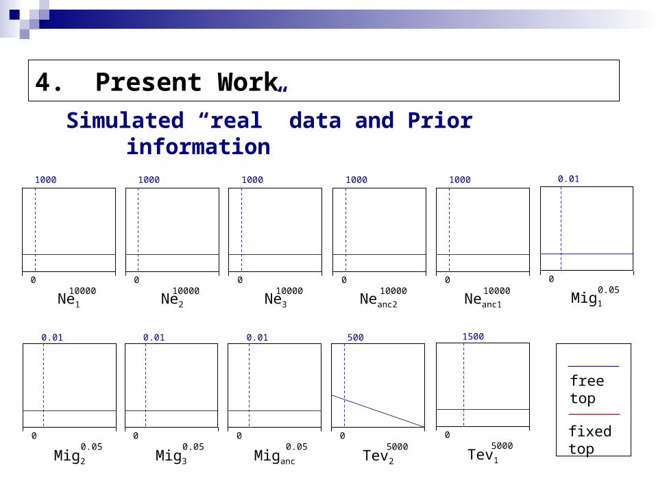
Simulated “real” data and Prior information
0 10000
1000 1000 1000
0 10000 0 10000 0 0.05
0 0.05
0.01
0.01
Ne1 Ne2 Ne3
Mig2
Mig1
free top
fixed top
500
0 0.05 0 0.05 0 5000
0.01 0.01
Tev2MigancMig3
1500
0 5000
Tev1
0 10000
1000 1000
0 10000
Neanc2 Neanc1
4. Present Work
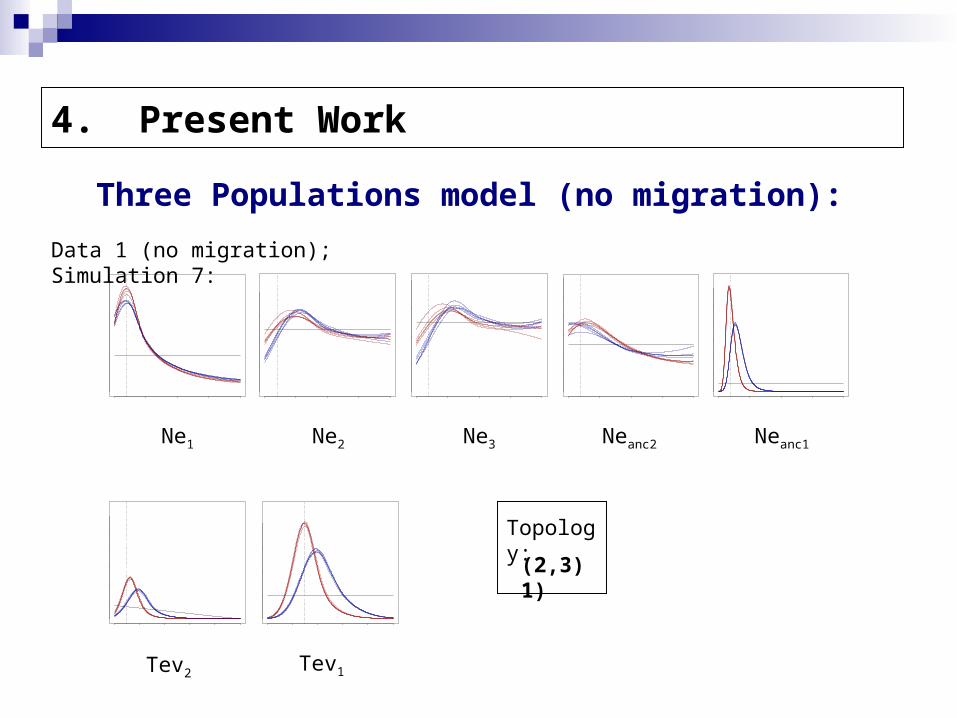
Three Populations model (no migration):
Ne1 Ne2 Ne3
Tev2 Tev1
Neanc2 Neanc1
Topology:
Data 1 (no migration); Simulation 7:
(2,3)1)
4. Present Work
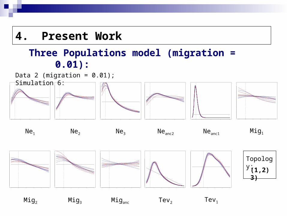
Three Populations model (migration = 0.01):
Data 2 (migration = 0.01); Simulation 6:
Topology:
(1,2)3)
Ne1 Ne2 Ne3
Mig2
Mig1
Tev2MigancMig3 Tev1
Neanc2 Neanc1
4. Present Work
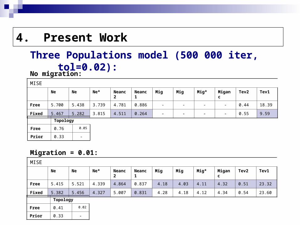
Three Populations model (500 000 iter, tol=0.02):
MISE
Ne Ne Ne* Neanc2 Neanc1 Mig Mig Mig* Miganc Tev2 Tev1
Free 5.700 5.438 3.739 4.781 0.886 - - - - 0.44 18.39
Fixed 5.467 5.282 3.815 4.511 0.264 - - - - 0.55 9.59
No migration:
Migration = 0.01:MISE
Ne Ne Ne* Neanc2 Neanc1 Mig Mig Mig* Miganc Tev2 Tev1
Free 5.415 5.521 4.339 4.864 0.837 4.18 4.03 4.11 4.32 0.51 23.32
Fixed 5.382 5.456 4.327 5.007 0.831 4.28 4.18 4.12 4.34 0.54 23.60
Topology
Free 0.76 0.05
Prior 0.33 -
Topology
Free 0.41 0.02
Prior 0.33 -
4. Present Work
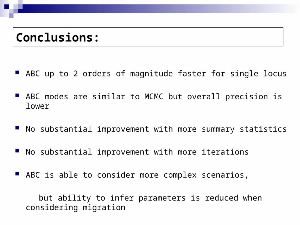
Conclusions:
ABC up to 2 orders of magnitude faster for single locus
ABC modes are similar to MCMC but overall precision is lower
No substantial improvement with more summary statistics
No substantial improvement with more iterations
ABC is able to consider more complex scenarios,
but ability to infer parameters is reduced when considering migration
1. Applications of ABC in population genetics2. Motivation for the application of ABC3. ABC approach
1. Characteristics of an ABC methodology2. Algorithm of an ABC inference3. Limitations of the ABC approach4. Typical ABC run
4. Present work1. Compare the ABC algorithm with a MCMC one2. Study the use of different summary statistics3. Study the use of ABC in more complex scenario4. “State of art” of the software
5. Future developments
Index
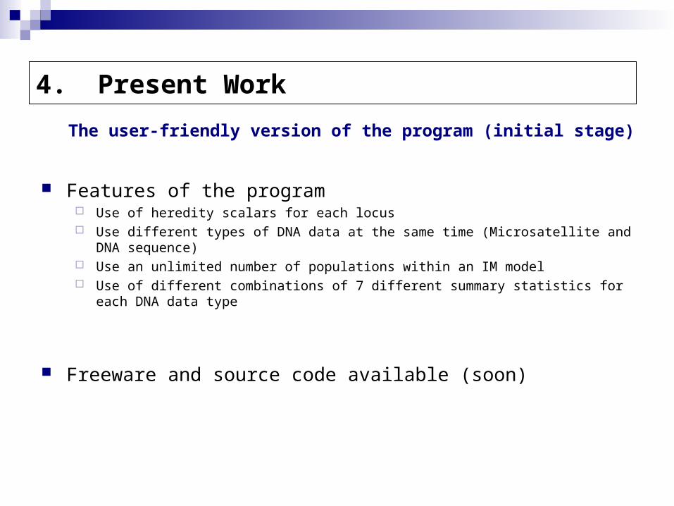
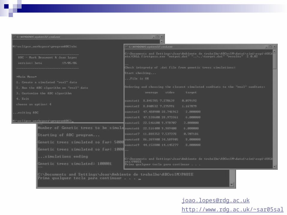
The user-friendly version of the program (initial stage)
Features of the program Use of heredity scalars for each locus Use different types of DNA data at the same time (Microsatellite and DNA sequence) Use an unlimited number of populations within an IM model Use of different combinations of 7 different summary statistics for each DNA data type
Freeware and source code available (soon)
4. Present Work
1. Applications of ABC in population genetics2. Motivation for the application of ABC3. ABC approach
1. Characteristics of an ABC methodology2. Algorithm of an ABC inference3. Limitations of the ABC approach4. Typical ABC run
4. Present work1. Compare the ABC algorithm with a MCMC one2. Study the use of different summary statistics3. Study the use of ABC in more complex scenario4. “State of art” of the software
5. Future developments
Index
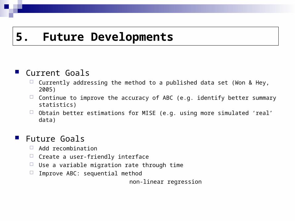
5. Future Developments
Current Goals Currently addressing the method to a published data set (Won & Hey, 2005) Continue to improve the accuracy of ABC (e.g. identify better summary statistics) Obtain better estimations for MISE (e.g. using more simulated ‘real’ data)
Future Goals Add recombination Create a user-friendly interface Use a variable migration rate through time Improve ABC: sequential method
non-linear regression
Acknowledgements
I would like to acknowledge David Balding for helpful discussion on the methods used. And also a special thanks to Mark Beaumont for advice and comments on the work.
Support for this work was provided by EPSRC.