Recap WTP Normalisations Special Reg

Introduction to Identification

Abi Adams

HT 2017

Abi Adams

TBEA

Recap WTP Normalisations Special Reg

Outline for Today

Aim: Understand basic concepts so that we can move on toapply them in a range of applied settings in future lectures

I Recap

II Normalisations (in the context of discrete choice)

III Special Regressors

Abi Adams

TBEA

Recap WTP Normalisations Special Reg

Recap

Abi Adams

TBEA

Recap WTP Normalisations Special Reg

Recap

Abi Adams

TBEA

Recap WTP Normalisations Special Reg

Recap: Observational Equivalence

Abi Adams

TBEA

Recap WTP Normalisations Special Reg

Recap: Point Identification

Abi Adams

TBEA

Recap WTP Normalisations Special Reg

Recap: Structural Features

Abi Adams

TBEA

Recap WTP Normalisations Special Reg

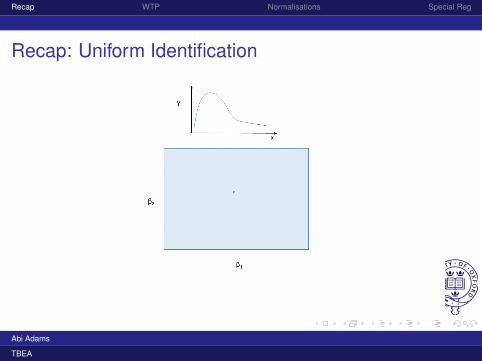
Recap: Uniform Identification

Abi Adams

TBEA

Recap WTP Normalisations Special Reg

Recap: Uniform Identification

Abi Adams

TBEA

Recap WTP Normalisations Special Reg

Recap: Terminology

I Observational Equivalence 1S′ and S′′ such that F S′

YX = F S′′

YX are observationallyequivalent

I Observational Equivalence 2S′ and S′′ such that F S′

φ = F S′′

φ are observationallyequivalent given the features of the data that are knowable,φ

I The model Γ identifies S0 if there is no S′ ∈MΓ such thatF S0

φ = F S′

φ

Abi Adams

TBEA

Recap WTP Normalisations Special Reg

Proving Identification

I There are a number of ways that one might demonstrateidentification

I The most common way is to prove identification byconstruction: given a structure, one is able to write aclosed form expression for θ as a function of φ

I However, not necessary that a closed form expressionexists for a structure to be identified

Abi Adams

TBEA

Recap WTP Normalisations Special Reg

Example: Identifying WTP

I Lewbel, Linton, McFadden (2011): want to recover thedistribution of people’s willingness to pay (WTP), W ?,FW?(w).

I Dataset used by Hanemann et al. (1991) to elicit the WTPfor protecting wetland habitats and wildlife in California’sSan Joaquin Valley

I For each person in the sample, researchers draw a price Pfrom a known distribution function and ask if they would bewilling to pay $P or more to preserve the wetland

Abi Adams

TBEA

Recap WTP Normalisations Special Reg

Example: Identifying WTPI Binary choice: D denotes an individual’s response

D = I (W ? > P) (1)

I Given random assignment of prices, P is distributedindependently of W ?

E(D|P = p) = Pr (W ? > P|P = p)

= Pr (W ? > P)

= 1− Pr (W ? < P)

= 1− FW?(p)

(2)

I Here, identification is proved by construction: FW? isuniquely determined by the function E(D|P = p), which isassumed to be known given φ

Abi Adams

TBEA

Recap WTP Normalisations Special Reg

Example: Identifying WTP

I Note that given the experimental design, the function FW?

might not be identified everywhere

I In the motivating experiment, P could take on one of 14values between $25 and $375 — can identify thedistribution function only at w? = p at these particularvalues

I To identify the entire distribution function FW? , would wantto design an experiment so that P could take on any valuethat W ? could equal — p should be drawn from acontinuous distribution with support at least as large as therange of possible values of W ?

Abi Adams

TBEA

Recap WTP Normalisations Special Reg

Proving Identification: Extremum

I Another common method is to prove that θ0 is the uniquesolution to some maximisation problem defined given S

I E.g. Show that the likelihood is globally concave, thenmaximum likelihood will have a unique maximising value

I Establish identification by showing that the uniquemaximiser in the population equals the true θ0

I Note trend to attempt to show this with complicatedstructural models by graphing marginal likelihood functionat the estimated parameter vector — don’t do this forpresentations!

Abi Adams

TBEA

Recap WTP Normalisations Special Reg

Discrete Choice

I The WTP Example provides some insight into specialregressor methods, often used in discrete choice modelswhen we want to be flexible about the distribution ofunobserved preference heterogeneity

I Before starting, a brief recap on discrete choice to allow usto discuss the role of normalisations

Abi Adams

TBEA

Recap WTP Normalisations Special Reg

Binary Choice

I Imagine a consumer choosing whether to consume agood/enter into treatment/start working

I Choose the action if:

α + βXi > εi (3)

I The probability that they choose

Pr(Yi = 1|X = xi) = Pr(α + βxi > εi |X = xi)

= Pr(α + βxi > εi)

= Fε(α + βxi)

(4)

Abi Adams

TBEA

Recap WTP Normalisations Special Reg

Binary Choice

I In most of the models you will have encountered thus far,you proceed by putting a functional formal assumption onthe distribution of the errors

I Example: Probit: εi ∼ N(µ, σ2)

I However, without further restrictions, {α, β} are notidentified

Pr(Yi = 1|X = xi) = Fε(α + βxi)

= Φ

(α + βxi − µ

σ

) (5)

Abi Adams

TBEA

Recap WTP Normalisations Special Reg

Binary Choice: LocationI Different combinations of {µ, α} are observationally

equivalent

Pr(Yi = 1|X = xi) = Φ

(α + βxi − µ

σ

)= Φ

((α + κ) + βxi − (µ+ κ)

σ

)= Φ

(α̃ + βxi − µ̃

σ

) (6)

I Standard: restrict µ = 0 — the location normalisation

Pr(Yi = 1|X = xi) = Φ

(α + βxi

σ

)(7)

Abi Adams

TBEA

Recap WTP Normalisations Special Reg

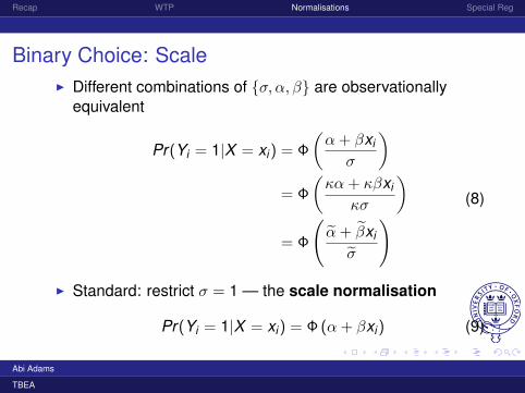
Binary Choice: ScaleI Different combinations of {σ, α, β} are observationally

equivalent

Pr(Yi = 1|X = xi) = Φ

(α + βxi

σ

)= Φ

(κα + κβxi

κσ

)= Φ

(α̃ + β̃xi

σ̃

) (8)

I Standard: restrict σ = 1 — the scale normalisation

Pr(Yi = 1|X = xi) = Φ (α + βxi) (9)

Abi Adams

TBEA

Recap WTP Normalisations Special Reg

Normalisations

I In parametric models, common to impose these restrictionson the distribution of the error term as we have just seen

I For example, in the Probit model above, assume that ε hasa standard normal distribution

I However, note that we could have imposed the locationand scale restrictions on {α, β} rather than {µ, σ}

I For example, α = 0 and βk = 1, allowing ε to have anarbitrary mean and variance

Abi Adams

TBEA

Recap WTP Normalisations Special Reg

Normalisations

I Normalisations common in semi- and nonparametricmodels

I Example: structure is a linear index model

E(Y |X ) = g(α + Xβ) (10)

I Features of interest: θ = {g, β, α}

I Normalisations/restrictions typically imposed on parametervectors in semiparametric models

Abi Adams

TBEA

Recap WTP Normalisations Special Reg

Normalisations

I For any nonzero constant κ, define θ̃ = {g̃, β̃, α̃} withβ̃ = β/κ, α̃ = α/κ and g̃(z) = g(κz)

I Then θ̃ is observationally equivalent to θ

I All elements β̃ in the identified set have β̃ proportional to β— identified up to a scale

I Require a scale normalisation, usually βk = 1 or β′β = 1

Abi Adams

TBEA

Recap WTP Normalisations Special Reg

Normalisations

I For any nonzero constant κ, define θ̃ = {g̃, β, α̃} withα̃ = α + κ and g̃(z) = g(z − κ)

I Then θ̃ is observationally equivalent to θ

I Require a location normalisation, usually α = 0 — excludea constant

Abi Adams

TBEA

Recap WTP Normalisations Special Reg

Normalisations

I What makes something a normalisation rather than arestriction?

I Calling a restriction a normalisation implies that is does notrestrict or limit behaviour — ‘without loss of generality’

I Thus, whether a restriction can be thought of in this waydepends in part on how we will use and interpret the model

Abi Adams

TBEA

Recap WTP Normalisations Special Reg

Normalisations

I If one is simply interested in, e.g. marginal effects, then thescale normalisation is indeed without loss of generality

∂Pr(Yi = 1)

∂X=β

σφ

(α + βX − µ

σ

)(11)

I If however want to imbue coefficients with meaning, onemight need to be careful!

I Caution: direct comparison of discrete choice coefficientsacross different samples/specifications

Abi Adams

TBEA

Recap WTP Normalisations Special Reg

Normalisations: Outside OptionsI ‘Outside option’ normalisations are also common in

discrete choice models

I Let utility from choice Y = y for y = 0,1

αy + βyX + εy (12)

I Utility maximisation means that choose good 1 if:

α1 + β1X + ε1 > α0 + β0X + ε0

(α1 − α0) + (β1 − β0)X + (ε1 − ε0) > 0α + βX + ε > 0

(13)

I Interpret α + βX as the utility from Y = 1 if assume thenormalisation that the utility of the outside option is zero

α0 + β0X + ε0 = 0 (14)

Abi Adams

TBEA

Recap WTP Normalisations Special Reg

Normalisations: Outside Options

I In static discrete choice models, this is usually a freenormalisation, without loss of generality

I However, this might not be the case in dynamic discretechoice models

I Assuming that the outside option has the same utility inevery period imposes real restrictions on preferences andhence on behaviour — be careful!

Abi Adams

TBEA

Recap WTP Normalisations Special Reg

Relaxing Assumptions on ε

I The parametric assumptions placed on the distribution ofunobserved errors are essentially arbitrary and can havevery restrictive behavioural implications

I To introduce some more common concepts in theliterature, explore the use of ‘special regressors’ in discretechoice and their role in identification

I Intuitively, variation in special regressors allow one to traceout the distribution of unobservables

Abi Adams

TBEA

Recap WTP Normalisations Special Reg

Special Regressor MethodsI Let’s pick up on the example from the beginning of the

lecture, casting in the standard notation used in theliterature:

D = I (W ? > P)

= I (W ? − P > 0)

= I (W ? + V > 0)

(15)

I Let H(v) = E(D|V = v) and suppose V is continuouslydistributed (V is the special regressor!)

H(v) = Pr (W ? + V > 0)

= Pr (W ? > −V )

= 1− FW?(−v)

(16)

I If the support of V contains the support of −W ?, then theentire distribution function FW? would be identified

Abi Adams

TBEA

Recap WTP Normalisations Special Reg

Special Regressor Methods

I Want to identify, e.g., the average willingness to pay; thespecial regressor allows one to do this

E(W ?) =

∫ wu

wl

wfw?(w) dw

=

∫ wu

wl

w∂Fw?(w)

∂wdw

=

∫ wu

wl

w∂ [1− H(−w)]

∂wdw

(17)

Abi Adams

TBEA

Recap WTP Normalisations Special Reg

Special Regressor Methods

I Key assumptions on the special regressor:I Independence (or conditional independence)

I Additive

I Continuity

I Large support

I Pop up a lot even if not always identified as specialregressors!

Abi Adams

TBEA

Recap WTP Normalisations Special Reg

Special Regressor Methods

I Large support important for identification of certainfeatures that rely on knowledge of the tails of a distribution

E(W ?) =

∫ wu

wl

w∂ [1− H(−w)]

∂wdw (18)

I If supp(V) bounded to a ≤ V ≤ b, then Fw?(w) onlyidentified for −b ≤W ? ≤ −a

I In this case, E(W ?) is not even set identified

I No bounds on E(W ?) because Fw? could have massarbitrarily far below −b or above −a

Abi Adams

TBEA

Recap WTP Normalisations Special Reg

Special Regressor: Random Coefficients

I Random coefficients often used to allow for moresophisticated unobserved preference heterogeneityspecifications

Y = I(V εv + X εx > 0) (19)

where εv and εx are random coefficients

I Assume εv > 0 and let ε = εx/εv — a scale normalisation

Y = I(V + X ε > 0) (20)

I Is the distribution of ε identified from the data?

Abi Adams

TBEA

Recap WTP Normalisations Special Reg

Special Regressor: Random CoefficientsI Assume that V is a special regressor, distributed

independently of X

Y = I(V + X ε > 0)

= I(V + U > 0)(21)

I Using the same argument as before FU|X is identified byvariation in the special regressor

E(Y |X = x ,V = v) = Pr(v + U > 0|X = x)

= 1− FU|X (−v)(22)

I So the distribution of ε is identified!

Abi Adams

TBEA

Recap WTP Normalisations Special Reg

Conclusion

I These two lectures have introduced the concept ofobservational equivalence and introduced its role inproving identification of structural features

I Next week we will consider the connection between this‘structural’ approach to identification and a ‘causal’approach to identification

I We will apply these results to consider identification insimple equilibrium settings

Abi Adams

TBEA