About strongly polynomial time algorithms for quadratic optimization
over submodular constraints ~
Dorit S. Hochbaum a,b,*, Sung-Pil Hong b a School ofBusinessAdministration, University ofCalifornia, Berkeley, CA, USA
b Department ofIEOR, University ofCalifornia, Berkeley, CA 94720, USA
Received 17 February 1993; revised manuscript received 18 July 1994
Abstract
We present new strongly polynomial algorithms for special cases of convex separable quadratic minimization over submodular constraints. The main results are: an O(NM log (N2 /M) ) algorithm for the problem Network defined on a network on M arcs and N nodes; an O(n log n) algorithm for the tree problem on n variables; an O(n log n) algorithm for the Nested problem, and a linear time algorithm for the Generalized Upper Bound problem. These algorithms are the best known so rar for these problems. The status of the general problem and open questions are presented as weil.
programs are those with 0-1 coefficients in the constraint matrix.) Separable convex quadratic optimization problems over "combinatorial" constraints are not known to possess strongly polynomial algorithms.
Solvability in strongly polynomial time for a linear or quadratic programming problem on n variables and m constraints means that there exists an algorithm that solves the problem in a number of steps that is bounded by a polynomial function of n and m only. The general optimization problem over submodular constraints can however be described without an explicit description of the constraints. Such is the case when there is a constraint for each subset of the universal set of n variables. The input then describes the rank function defined on all possible subsets of the universal set. In this case, for an algorithm to be strongly polynomial, its running time depends on n alone, and the length of the description of the rank function.
Although combinatorial Linear Programming problems are solvable in strongly polynomial time, this feature is not shared with nonlinear problems. In [17], it was shown that nonquadratic concave separable optimization problems are not solvable in strongly polynomial time in a computation model that includes the arithmetic operations, comparisons and the floor operation. This lower bound was illustrated for the simple
resource allocation problem max{~~= 1 f j ( x i ) ]~nj= a xj ~< B, x >/0, x integer}, and for its continuous version. The simple resource allocation problem is the simplest form of nonlinear optimization over submodular constrains. This negative result applies only for nonquadratic objective functions, so the issue of the strong polynomiality of quadratic optimization problems over linear constraints is still open.
While for a general optimization problem there is a clear distinction in complexity between optimizing over integers or over continuous variables, this is not the case for optimization over submodular constraints. It is proved in [17] that there is a "proximi ty"
theorem between an optimal integer and optimal continuous solution to the problem where any optimal continuous solution rounded down bounds from below an integer optimal solution. This allows in particular to solve the integer problem by solving first the continuous problem and then apply what amounts to at most n steps to reach an optimal integer solution. This strategy is adopted throughout this paper in order to derive continuous and integer solutions to the quadratic optimizätion problem over submodular constraints.
Known cases where convex quadratic optimization in integers (or continuous vari- ables) over linear constraints can be solved in strongly polynomial time include: a nonseparable quadratic transportation problem [19]; an unconstrained nonseparable quadratic optimization in the context of electrical distribution system [1]; a nonseparable problem in the context of toxic waste disposal [15]; a quadratic continuous Knapsack problem [4]; a problem where the constraints consist of two equations and lower and upper bounds [2]; a transportation problem with fixed number of sources (of sinks) [6]; an improvement in complexity to the transportation problem with fixed number of sources and extending the strong polynomiality to a quadratic problem over a fixed number of equations [21]; a quadratic series-parallel network with a single source and sink [23].
Our aim in this paper is to establish the most efficient strongly polynomial algorithms known for several quadratic problems over submodular constraints. The general quadratic problem over submodular constraints is defined with respect to some submodular rank function r : A ~ R defined on a distributive lattice A of E = { 1 , . . , n} (a set of subsets of E which contains ¢, E and is closed on the set intersection and union), i.e. r(~) = 0
and for all A,B ~ A,
r(A) + r(B) >~ r(A UB) + r(A AB) .
(For a detailed description of submodular functions see e.g. [22].) The submodular polyhedron defined by the submodular function r is the set {xlEj~ Ax t <~ r(A), A ~ A}.
We call the system of inequalities {F~j~Axj<r(A)IA~A}, submodular con- straints. The problem of quadratic integer optimization over submodular constraints is
then,
min 1 2 E ajxj + ~bj~j j ~ E
~_,x j<r(A) , A ~ A jEA
xj >~ 0 and integer, j ~ E.
For b a nonnegative vector, the objective function is convex. This is a special case of the convex nonlinear problem over submodular constraints, the general resource allocation problem or (GAP):
(GAP) max ~ ~.(xj) j~E
~_,xj<~r(A), A ~ A j~A
xj >~ 0 and integer, j ~ E.
The problem (GAP) was proved polynomial by Groenevelt [16], using the ellipsoid algorithm, and by Hochbaum [17] nsing a proximity and scaling based algorithm. Since the number of constraints in the problem could be exponential in [ E I, the running time is expressed in terms of the number of calls to an oracle that determines whether a solution is a member of the submodular polyhedron, or equivalently, feasible for the
submodular constraints. Let F denote the number of steps that an oracle requires to determine whether incrementing a given feasible solution vector in one of its compo- nents by one unit results in a feasible solution vector. The running time given in [17] is O(n(log n + F)log2(r(E)/n))), and for the confinuous case an e-accurate solufion (within « in the solntion space) is produced in O(n(log n + F) log2(r(E)/en)) steps. (There is no statement of running time in [16].) Note that this running time is
polynomial, but not strongly polynomial as it depends on the value of the right-hand side, r(E). These algorithms apply particularly to the problem of quadratic optimization
The problem (GAP) has been studied extensively in the literature. A book by Ibaraki and Katoh [20] presents an excellent state-of-the-art survey on this problem and its special cases. Here we focus on the instances of the problem where the objective function is quadratic. We present here strongly polynomial algorithms for all cases of (GAP) studied in the literature. These problems, in addition to the simple resource allocation problem, (SRA), are the generalized upper bound resource allocation prob- lem, (GUß), the nested resource allocation problem, (Nested), the tree resource allocation problem, (Tree), and the network resource allocation problem, (Network). The definitions and formulations of these problems are given in Section 2.
Prior work on strongly polynomial algorithms for the problems discussed here includes two algorithms. In [9], Fujishige devised an algorithm for the lexicographically optimum flow problem from which it is possible to derive an O(N2M log(N2/M)) time algorithm for (Network) when the underlying network has M arcs and N nodes, and hence for all other problems described here. This algorithm, when applied to (Tree), runs in O(n 2) time. Another algorithm by Tamir [23], solves the minimum convex separable quadratic cost flow problem on series-parallel network for which (Tree) is a special case. Applied to the problem (Tree), this algorithm has complexity O(n2).
The main results here are an O(NM log(N2/M)) algorithm for (Network), an O(n log n) algorithm for (Tree) on n variables, an O(n) algorithm for (Nested) when given a sorted array of the coefficients, a j, and a linear time algorithm for (GUß). These results constitute therefore a significant improvement on the complexity of currently available algorithms. Such efficient algorithms also lend additional support to the conjecture that the problem of quadratic cost network flow is solvable in strongly polynomial time.
The paper is organized as follows. Section 2 defines the classes of problems addressed and gives their formulations. In Section 3 we give the algorithm for the quadratic simple resource allocation problem that is used as building blocks for the nested and tree algorithms. Section 3 also describes the linear time algorithm used for the generalized upper bounds problem. Section 4 contains the algorithm for (Nested), and Section 5 contains the algorithm for (Tree). Section 6 describes the algorithm used for the (Network) case, and our implementation of a parametric flow algorithm.
2. Formulations and preliminaries
2.1. Formulations
Important special cases of optimization over submodular constraints that have been studied in the literature are formulated here with a quadratic objective function. The formulations given here include a constraint for the rank of the entire set as an inequality constraint. However, all the algorithms given in this paper can be easily modified to
solve the corresponding problem given with this constraint as an equality. The problems are also slightly generalized by allowing upper bound constraints on the variables.
We assume throughout that the objective functions are strictly convex, that is, the vector b is positive. This assumption is made for the sake of convenience of the presentation. All algorithms described apply also when some of the functions are linear with an obvious modification. For the network problem, where the modification is less obvious, there is a discussion on the method of modifying the algorithm. We choose not to treat the non-strictly-convex cases explicitly, in order not to obscure the main algorithmic issues involved.
(1) The simple resource allocation problem:
(SRA) min I 2 ~ ajxj + 7bjxj j = l
B xj<~ß j = l
0 ~ xj ~< uj integers, j = 1 , . . , n .
The problem (SRA) may be viewed as a minimum cost flow problem with a source that has supply of B units. Each variable represents the amount of flow along each arc going from a node to a sink t. There are no costs or capacities associated with the arcs going into the nodes other than the sink, but there are capacity upper bounds uj associated with the arc going from node j to the sink and also quadratic cost functions
1 2 ajxj + -~bjxj. Since the "supply" in the formulation above is up to B, this can be incorporated by adding an arc with zero cost (and infinite capacity) from source to t. Such arc is omitted from the network described in Fig. l(a). Note that (SRA) could also be considered as a quadratic transportation problem with a single supplier and n customers. This observation underlied the technique used in [6] for solving quadratic transportation problems.
(2) The generalized upper bound resource aUocation problem:
( GUB ) min 1 2 B ajxj + 2bjxj j = l
B xj ~<B j= l
E x j ~ p i , i = l , . . . , m j~S i
0~<xj~<ujintegers, j = l . . . . ,n.
where {S 1, S 2 . . . . . Sm} is a partition of E = {1 . . . . , n}, i.e. disjoint sets the union of which is E. A depiction of this problem as a minimum cost flow problem is given in Fig. l(b).
274 D.S. Hochbaum, S.-P. Hong /Mathematical Programming 69 (1995) 269-309
~ ~ \ v C v ~ x "c
\ \ x - - - ~ " ,.,~ g • . - / / ~ " / ( [ / I ° o. \ .~
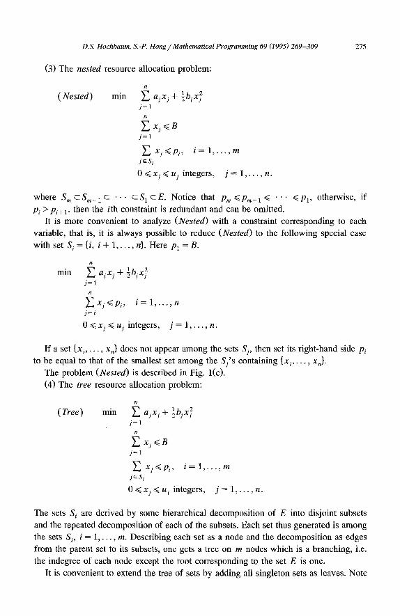
where S m c S m_ 1 c • • • c S 1 c E. Notice that Pm ~ Pro- 1 ~< " " " ~< Pl , otherwise, if Pi > Pi+ 1, then the /th constraint is redundant and can be omitted.
It is more convenient to analyze (Nested) with a constraint corresponding to each variable, that is, it is always possible to reduce (Nested) to the following special case
with set S i = {i, i + 1 . . . . . n}. Here Pl = B.
min ~~xj + lbjx~ j = l
BXj<~Pi , i = l , . . . , n j=i
O~<xj~<ujintegers , j = l , . . . , n .
If a set {x i . . . . . x n} does not appear among the sets Sj, then set its right-hand side Pi to be equal to that of the smallest set among the Sj's containing {x i , . . . , Xn}.
The problem (Nested) is described in Fig. l(c).
(4) The tree resource allocation problem:
(Tree) min 1 2 B ajxj + ~bjxj j = l
B xj ~ B j = l
E Xj<~Pi, i = l , . . . , m j~S i
O <~ xj <~ uj integers, j = l , . . . , n .
The sets S i are derived by some hierarchical decomposition of E into disjoint subsets and the repeated decomposition of each of the subsets. Each set thus generated is among the sets Si, i = 1 , . . , m. Describing each set as a node and the decomposition as edges from the parent set to its subsets, one gets a tree on m nodes which is a branching, i.e. the indegree of each node except the root corresponding to the set E is one.
It is convenient to extend the tree of sets by adding all singleton sets as leaves. Note
that the problem could be viewed as flow problem from the root to the leaves where the objective function minimizes the quadratic cost of the flow to the leaves only. All other flows have cost of zero, and only the capacitated nodes and the flow balance constraints determine the feasibility. The network describing the flow problem corresponding to the tree allocation problem is given in Fig. l(d).
(5) The network resource allocation problem is defined with respect to any network (or graph), with a single source and a set of sinks.
Given a directed graph (network) G = (V, A) with node set V and arc set A. Let s E V be the source and T ___ V be the set of sinks. The supply of the source is B > 0, and the capacity of arc (i, j ) is Cij. Denote the flow vector by f = {f/j [(i, j ) GA}
1 2 (Network) min ~ akx k + 2bkxk tk~ T
E fij-- E fji =0' i ~ V - - T - - { s } (i,j)EA (j,i)~A
E Lj<8 (s,j)~A
E ~,~- E Lj=x~, (j,tk)~A (tk,j)~A
0~<f/ j~<cq, ( i , j ) GA
O <~ x~ < u k, tk ~ T.
t h ~ T
Given a feasible flow f in G, each variable x k represents the net value of the flow arriving at the sink t k. We call x the out-flow vector of the flow f. The (quadratic) network resource allocation problem (Network) is not the same problem as the minimum quadratic cost flow problem. In the latter problem there is an underlying graph and a quadratic cost associated with the flow along each arc. In this problem the quadratic costs are associated only with the flow x k arriving at each sink te. An alternative representation is to augment G with a dummy sink t, and connect each sink
t h to t with a directed arc (th, t) of capacity u k. The costs are then only associated with the arcs (th, t). All other arcs have 0 cost associated with them. This graph is described in Fig. l(e).
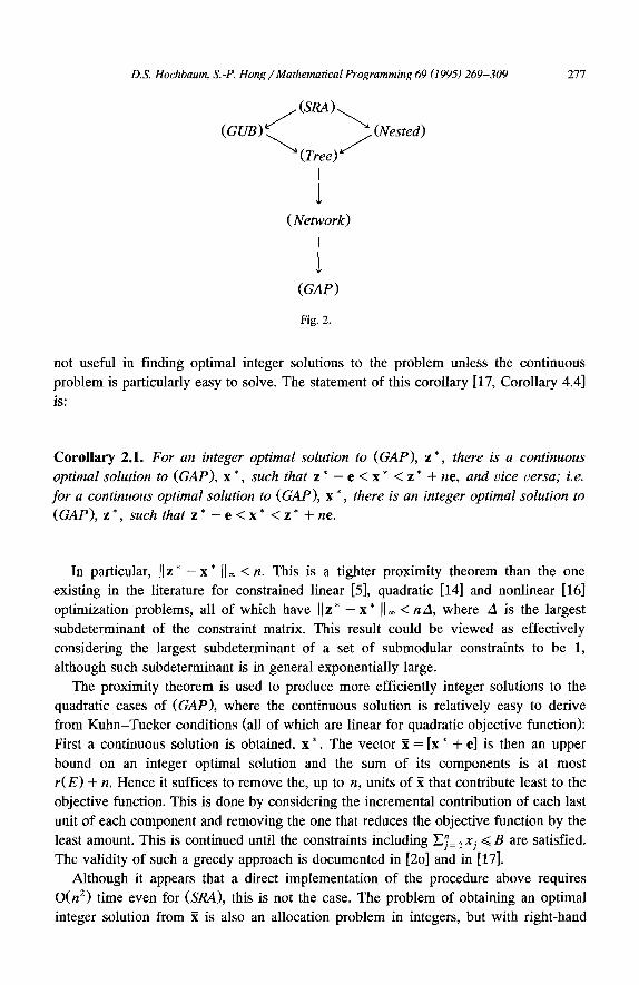
The relations between these problems are depicted in Fig. 2 where A ~ B if problem
A is a special case of problem B.
2.2. Deriving integer from continuous solutions
Vectors in this paper are denoted by boldface letters. The vector e denotes the n-vector (1 . . . . . 1).
A theorem in [17] states a proximity between an optimal (integer) solution to (GAP) and a scaled solution. A corollary of this theorem is a proximity result on the distance between an optimal integer and optimal continuous solutions to (GAP). Such result is
not useful in finding optimal integer solutions to the problem unless the continuous problem is particularly easy to solve. The statement of this corollary [17, Corollary 4.4]
is:
Corollary 2.1. For an integer optimal solution to (GAP), z *, there is a continuous
optimal solution to (GAP), x *, such that z * - e < x * < z * + ne, and vice versa; i.e.
for a continuous optimal solution to (GAP), x *, there is an integer optimal solution to
(GAP), z* , such that z * - e < x* < z* + ne.
In particular, Hz* - x * ][~ < n. This is a tighter proximity theorem than the one existing in the literature for constrained linear [5], quadratic [14] and nonlinear [16] optimization problems, all of which have []z * - x * [la < nA, where A is the largest subdeterminant of the constraint matrix. This result could be viewed as effectively considering the largest subdeterminant of a set of submodular constraints to be 1, although such subdeterminant is in general exponentially large.
The proximity theorem is used to produce more efficiently integer solutions to the quadratic cases of (GAP), where the continuous solution is relatively easy to derive from Kuhn-Tucker conditions (all of which are linear for quadratic objective function):
First a continuous solution is obtained, x *. The vector ~ = [x * + e] is then an upper bound on an integer optimal solution and the sum of its components is at most
r ( E ) + n. Hence it suffices to remove the, up to n, units of ~ that contribute least to the objective function. This is done by considering the incremental contribution of each last
unit of each component and removing the one that reduces the objective function by the least amount. This is continued until the constraints including ~~= 1 xj ~< B a r e satisfied. The validity of such a greedy approach is documented in [20] and in [17].
Although it appears that a direct implementation of the procedure above requires O(n 2) time even for (SRA), this is not the case. The problem of obtaining an optimal integer solution from '~ is also an allocation problem in integers, but with right-hand
sides that are O(n). Such allocation problems, if they have same constraints as the problems in Subsection 2.1, with any convex separable objective function, are solvable with the following running times:
(SRA) in O(n), [8], (GUß) in O(n), [17], (Nested) in O(n log n) [17], (Tree) in O(n log n) [17], (Network) and any submodular constraints, in O(nF) where F is the number of steps
required to check whether an increment of one unit (of flow, in (Network)) is feasible. These running times are added to the complexity of the continuous problem in order
to determine the complexity of the integer problem. Yet, in all cases these running times are dominated by those required to solve the continuous problem. Thus in the subse- quent part of this paper, we consider only the continuous versions of the problems defined in the previous subsection.
3. A linear time algorithm for (SRA) and (GUß)
Brucker [4], was the first to devise a linear time algorithm for the continuous convex quadratic Knapsack problem. This problem is more general than (SRA) in that its constraint may have nonnegative coefficients to the variables where in (SRA) all these coefficients are 1. The algorithm presented here is also directly applicable to the Knapsack version of the problem with a minor adjustment. The presentation here follows the algorithm given in [6] with some appropriate modifications.
At the optimum of (SRA) the derivative with respect to each variable has to be nonpositive. (Otherwise, a variable with positive derivative value at the optimum can be decreased by e > 0 while only improving (reducing) the objective function and without violating any constraint.) In other words, xj <~ max{0, - a J b j } . Hence we can update uj ~ min{uj, max{0, - a Jb j}} for each j and then B ~ min{B, E~= luj} without affect- ing the optimality. Also, notice that with this preprocessing, taking O(n) time, at any optimal solution, F~7= l Xi <~ B is binding. Otherwise there should be a variable with value less than the (updated) upper bound and hence with a negative derivative. Then we can increase the value of the variable by a small amount to reduce the objective value while maintaining the feasibility, contradicting to the optimality assumption. Thus by a linear time preprocessing, (SRA) is reducible to the same problem with equality constraint:
1 2 (SRA) min Æ ajxj + 7bjxj j=l
~ x j = B j=l
O<~xj<~uj, j = l , . . . , n ,
where B is positive, B ~< E7 = 1% and each bj is positive.
The convexity of the objective function guarantees that a solution satisfying the Kuhn-Tucker conditions is also optimal. In particular, we seek a nonnegative solution x * and a value 6 * such that
xj = B and u j > x j > 0 ~ ay + b i x j = 6 " . j = l
The situation is illustrated by Fig. 3. The value set for 6 determines associated values for xj. For any value 8, the
associated solution x(6) is
/ O
x j ( 6 ) = ( 3 - a j ) / b j
I, uj
if 8 ~< a j,
if aj < ¢~ <~ aj + bj U j ,
if aj + bjuj < 3.
(3.1)
Let / ~ ( 8 ) = F.,~=lxj(6). Then finding the optimal solution to (SRA) is equivalent to ~< n finding a value 8 * such that /}(6 * ) = B. (Since 0 < B ~ ~j= luj, it follows that there is
a finite optimal 6 * for every instance of (SRA).) Notice that /}(8) is a monotone increasing, piecewise linear function of 8, having
breakpoints at the values ai, and aj + bjuj for j = 1 . . . . . n. So if /~(8) < B , then we could conclude that 6 * is greater than 6 and similarly, i f / ~ ( 6 ) > B, then 6 * is less than 6. Thus the monotonicity o f / 3 ( 6 ) allows for a binary search for the optimal value, 6 * satisfying /~(8) = B.
The algorithm we propose for finding 3 *, chooses "guesses" (from among the breakpoint values, aj and aj + b j u ) until it finds two consecutive breakpoints which contain 6 * in the interval between them. In this range, /}(8) is a linear function. The problem is then solved by finding the particular value of 6 for which /} (8) = B (i.e., by solving the linear equation in one variable).
/ ~ ( 6 ) = 6 E 1 E ~ + E u j , (3.2) j ~ u bj j ~ u oj j c v
where U = {j I aj < 6 ~ aj + bjuy} and V = {j[ aj + bjuj < 6}. So at each iteration, we need to determine the index sets and the corresponding sums.
To result in a better complexity, the algorithm avoids computing the index sets and the sums at every iteration from scratch. For this purpose, it maintains the parameters P, Q and R which retain partial sums from the previous iteration.
Procedure SRA
Step 0: {initialization} S ~ { a 1 . . . . , a~; a 1 + b l U l , . . , a,, + bnun}. I, J ~ {1 . . . . . n}, P ":--~,~=laj/bj, Q <---2~7=11/b r
Step 1: {selecting median of breakpoints} Set 6 to be the median value from the set S. {computing coefficients of/~(i~)} L(~)<---{j ~ I [ ~<~ aj}, R ( ~ ) ~ {j E J l a j + bjuj < ~}, M ( 8 ) ~ L ( ~ ) U R( ~) t3 ~ P - Ei E M(g)ai/bi, Ô ~ Q - Ei ~ M(g)l/bj, 1~ ~ Ej ~ R(g)uj.
Step 2: {computing-~(g)) ~ ,z gO _ ~ + ~. I f /~ ~- B then STOP, 6 * ~ 6. I f / ~ > B then 6* < 6 . I f / ~ < B then 6" > 6 .
Step 3: {update index sets, breakpoints and partial sums} If 6" < 6 then
I ~ I - L ( 6 ) , J ~ R(6) , S ~ {ay[j ~I} t .3{ay + byu~b j ~ J } .
If 8 = a,ù for some m, then P ~ P - am/b m, Q ",- Q - 1 / b m. Else {6* > 6},
I ~ L(6), J ",- J - R(~) , S ~- {aj[ j ~ I1 t3 {aj + bjujl j ~ J}. Step 4: {repeating until final interval is found}
If [S[ >i 2, go to Step 1. Else, 6* ~ (B +/~ - / ? ) / Q .
The algorithm outputs a value 6 *. Then the optimal solution is x(6 * ) which can be determined in linear time using (3.1).
Theorem 3.1. Procedure S R A finds 8 * and x* in O(n) time.
Proof. To prove the validity of Procedure SRA, we need to show the correctness of /~ in Step 2, which is the value of /~(6) for 6 = 6.
Consider Q in Step 1, which is the slope of the piecewise linear curve, /~(6), at 6 = 6. To compute Q, we first calculate Q which represent the maximum possible value
D.S. Hochbaum, S.-P. Hong / Mathematical Programming 69 (1995)269-309 281
of the slope o f /~ (6 ) when 6 takes value among the breakpoints of S. Thus, initially Q is ET= il~bi. From (3.2) and the definitions of L(6) and R(6), it follows that M(6) is the set of indices j such that 1~bi needs to be subtracted from Q to obtain the correct slope o f / 3 ( 8 ) for 8 = 6. Therefore, Q should be
1 1 1 1 z - = ~ - - z - = Q - ~ - (33)
Hence the coefficient Q calculated in Step 1 is correct for the first iteration. If 6 * < ~, then the next guess is the median of the lower half of the current
breakpoints, that is, those breakpoints less than 6. So in Step 3, the upper half of the current breakpoints (including the current guess ä) is deleted from the set S and in Step 3 S is updated accordingly. In this case Q, the maximum possible slope o f / ~ ( a ) over the updated S, is ô - aj /b mi f g = a m for some m, or O, otherwise. Furthermore, from the updated set I and J in Step 3 it follows again that M(/~) is the set of indices j such that 1~bi needs to be subtracted from (the updated) Q to obtain the correct slope of /~(6) for 6 = 6 in the next iteration. Thus the correctness of Q obtained in Step 1 follows by induction on the numbers of iteration.
On the other hand, if 6 * > 6, then the next guess is the median of the upper half of the current breakpoints. So, in this case, we use the same Q in the next iteration. Similar inductive arguments for/~ and /~ show the correctness of the computation o f / ~ ( 6 ) in Step 2.
When S contains only one element, say aj (or, aj + bjuj), then we can conclude that 6 * is between 6 and aj (or, aj + bjuj,^respectively). Furthermore, since /~ is a linear function of 6 in this range, (i.e. B = Q 6 - / 3 +/~), 6 * and x * are determined as in Step 4.
The O(n) complexity of the algorithm follows from the fact that each of Step 1, 2 and 3 can be pefformed in a number of arithmetic operations that is linear in the cardinality of the set S, including the selection of the median value [3]. Since the number of elements in the set is initially 2n and is cut in half after each pass, the total work is linear in (2n + n + n / 2 + n / 4 + • • • ) = 4n, so the complexity of the algorithm is O(n). []
The problem (GUß) is easier to handle once we observe that it is polynomially equivalent to a number of simple resource allocation problems. Consider the set S i, the constraint Ej E si xj ~< p» and the following simple resource allocation problem restricted
to Si: 1 2 ( SRAi) min Y'~ ajxj + ~bjxj
jESi
E Xj ~ Pi jES i
O<~xj, j ~ S i.
Lemma 3.2 (Hochbaum [17]). Let the solution to (SRA i) be {x~i)}j ~ s~. Then there exists an optimal solution to (GUß), x *, satisfying x 7 <~ x~ i) for all j ~ S i.
Remark. In [17], the lemma is proved for the discrete version of the problem. It is easy to see the proof is modified for the continuous version of the problem. This lemma is generalized and proved for the (continuous) (Tree) problem in Corollary 5.2.
Lemma 3.2 implies that once an optimal solution, {x~i)}j~si has been obtained for (SRA i) for every i = 1 , . . . , m, an optimal solution of (GUB) can be found by solving the following problem, (UB), which is also an (SRA).
n 1 2 (UB) min 2., ajxj + ~bjxj
j=a
~ x j = B j=l
0 <~ xj <<. min{uj,x~i)}, j = 1 . . . . . n.
It is therefore sufficient to solve each of the (SRA i) problems, in order to derive the upper bounds. Then to solve the problem (UB). The running time of such procedure is O ( n l ) q- O ( n 2 ) + • • • q- O(n m) = O ( n ) , followed by the linear time required to solve the resulting (UB) (which is an (SRA)).
4. An O(n log n) algorithm for (Nested)
The algorithm proposed here solves the problems (Nestedn), (Nes ted ,_1) , . . . , (Nested1), where (Nested i) is the problem,
,,e,, 1 2 ( Nestedi) , min 2., ajxj + ~byxy
j=i
~ x j < ~ p k , k = i . . . . . n
O<~xy<~uj, j = i . . . . . n.
Let an optimal solution to (Nested i) be x (i). Several properties of (Nested i) are essential in order to establish the correctness of the algorithm. The next lemma states that for the problem (Nestedi), the constraint y'n .x(i) - - j = ~ - j <~Pi may be assumed to be satisfied with equality. The proof is given for the analogous lemma, Lemma 5.3 for the tree resource allocation problem, (Tree), which generalizes (Nested).
Lemma 4.1. In (Nestedi) , by updating uj ~ min(uy, max( - a j / b y , 0}) for j = n, n - 1 . . . . . 1 and pj ~ min{py, Py+I + uj} for j = n - 1, n - 2 , . . . , 1, we may assume that the constraint S,~= i x~ i) <~ Pi is satisfied with equality.
The following lemma contains the key idea of the algorithm. The proof is postponed to Section 5 where it appears as Corollary 5.2.
D.S. Hochbaum, S.-P. Hong / Mathematical Programming 69 (1995) 269-309
Lemma 4.2. x~i) <~ ~ (i+O.vj , for j = i + l, . . . , n.
283
This lemma implies that the value of the optimal solution for (Nestedi+ 1) is an upper bound on the value of the variables, xi+ 1, xi+ 2 , . . , xn in (Nestedi). The upper bounds at each (Nested i) problem solved, uj can then be updated to u~ i) --- min{uj, x~ i+ 1)}, for j--- i + 1 , . . , n. Since {x~ i÷1)} satisfy constraints i + 1 . . . . , n, these constraints no longer need to be explicitly incorporated. Hence (Nested~) is equivalent to the problem
( Nested i) min 1 2 B ajxj + 7bjxj j= i
n
E Xj = Pi ]=i
O<~xi~u ~
0 ~ xj «. min{u,,x} i+ 1)}, j = i + l , . . . , n .
This latter formulation of the problem is an (SRA). The algorithm solves recursively the problems (Nested~) for i = n . . . . . 1 where at each call the optimal solution derived from the previous call is used as upper bounds to the variables in the current call. The optimal solution of (Nested~+ 1) is then used to derive an optimal solution to (Nested i) in constant amortized running time.
The problem (Nested~) is an (SRA). This suggests immediately an algorithm that requires linear time with each call using Procedure SRA. Such algorithm would result in complexity of O(n2). In order to get a more efficient approach, we maintain all information obtained in previous iterations on the status of the breakpoints previously considered. These breakpoints are also maintained in a sorted array. The need to maintain a sorted array adds an additive preprocessing step. The algorithm runs coefficients {a l , . . . , a n} is available with
factor of O(n log n) to the running time at a in linear time when the sorted sequence of the input.
The algorithm produces a Lagrange multipliers 8 for each (SRA), (Nested i) for i = n . . . . ,1. Let the Lagrange multiplier for (Nested i) be 8/. Unlike Procedure SRA which finds 6 by binary search, testing /3(8) on the median of the current (unsorted) breakpoints, the algorithm finds 8 by "linear search", testing /~(8) on consecutive elements of the current breakpoints given in sorted array. That is, starting with an initial guess, it continues to test the immediate successor (or predecessor) of the current guess until it finds the final interval.
The initial guess for 8 i is 8i+ 1. All variables xj for j = i + 1 . . . . , n are fixed for any 8 >t 8i+ 1 in testing since, by Lemma 4.2, the optimal solution of (Nested i) is bounded by the optimal solution of (Nestedi+~). So if 8 i> 8i+» then there are only O(1) arithmetic calculations required to find 6i as there are at most two breakpoints to be tested; namely, ai and a~ + bit t i. 8 i is then added to the top of the sorted sequence of breakpoints for the testing to solve (Nestedi_l). The crucial property is that when
Let the set of the Lagrange multipliers, T, be {8il , 8i2 . . . . , 8iq}; iq+ 1 ~--n + 1. F o r p = q , q - - 1 . . . . . 1, do
xj = max{ 8ip/by - ay/bj, 0} for j = i p , . . . , ip+l - 1.
Procedure Nested(i)
Input:
Step O: Step 1:
Step 2:
Step 3:
Step 3(a):
Step 3(b):
Step 3(c):
Two sorted sequences S and T. For each 6y, the values of P(6j), Q(~j) and U(Sy).
{trivial case} If a i > 0; stop, 8 i = 8i+ 1. {Check if 8 i is larger or smaller than 8i+ 1}
If Pi+l q- min{(S/+l - a g ) / b i , ui} <Pi, then 8 i > 8/+1; go to Step 2. If Pi+l + min{(8i+l - ag)/bi, ui} ~-Pi, then 8 i = 8i+1; substitute the breakpoint label 8g by 8i+1;
P( 8 i) '~-'- P ( 8 i + 1) + ag/b i, Q( Si) ~-- Q(8i+ 1) + l / b i , U( 8 i) ~-- U(S/+ 1); stop.
If Pi+l "-}- min{(8i+l - ag)/bi, ui} >Pg, then 8 i < 8i+ 1; remove 8i+ 1 from the top of T;
P ~ P ( 8 i + l ) , Q ~ Q(Si+l); U ~ U(Si+l); go to Step 3.
{8 i > 8i+ 1} Solve for 6, (8 - ai ) /b i =Pi --Pi+l"
8 i ~ 8, P ( 8 i) ~ ai/b » Q(8) ~ 1~bi, U(8/ ) ~Pi+~. Add a~ to the sorted sequence S; add 6 i to the top of T; stop.
{8 i < 6i+ 1} I f a i + biu i < 8 i + 1 then add a i and a i + biu i to the sorted sequence S;
U ~ U( 6i+ l) + u i. Else, a d d a i to S; P ~ P(8i+ 1) + ai /bi , Q ~ Q( 6i+ 1) + 1 / b i. Let the largest breakpoint lower than 6g+ 1 be v. If v an aFbreakpoint then go to Step 3(a). If v an (ay + bjuy)-breakpoint then go to Step 3(b). If v a 6~-breakpoint then go to Step 3(c). Let the breakpoint be a k, set 6' = a«. If 8 ' Q - P + U < p i then 8 i> 8'; go to Step 4. If 6 'Q - P + U >pi then 6 i < 6'; remove a k from top of S;
P *-- P - a k / b » Q ~ Q - 1/b~; go to Step 3.
If 6 ' Q - P + U = p i , then 6 i= 6'; stop. Let the breakpoint be a« + bku k, set 6' = a k + bku k.
If 6 ' Q - P + U < p i then 6 i> 8'; go to Step 4. If 6 ' Q - P + U > P i then 6g< 8'; remove a k + b ~ u k from top of S;
U ~ U - u«; go to Step 3. If 6 ' Q - P + U = p » then 8 i = 6'; stop. Let the largest breakpoint be 6k; set a' = 8«.
If 8 ' Q - P + P k <Pi then 8 i > 6'; go to Step 4.
If 6 'Q - P + pk > Pi then 6 /< 6'; P ~ P + P(6 ' ) , Q ~ Q + Q(6') , U ~ U - ( 6 ' Q ( 6 ' ) - P(6 ' ) ) ;
remove 6 k from top of the sequence T; go to Step 3.
If 6 ' Q - P + P k =Pi then 6i = 6'; stop. {6/> 8'} Solve for 8, 6 Q - P + U = p / .
Set 6 /= 8, P ( 6/) = P , Q( 6 i) = Q, U( 6 i) = U; stop.
L e m m a 4.3. Algor i thm Nested is correct. With a given sorted sequence o f
{a 1 . . . . . an; a 1 + b l U l , . . . , a n + bnun}, its complexity is O(n).
Proofi The dominant operation in the algorithm is adding element a i and biu / to the sorted sequence S in Step 3. Using a straightforward approach of binary search, this takes O(log n) comparisons. We adopt here the UNION-FIND algorithm of Gabow and Tarjan [11]. Each subsequence is viewed as a collection of intervals that contains NO elements of a/ or a i q- biui, with endpoints at elements of the subsequence. Alterna-
tively, the sorted sequence on { a l , . . . , an; a z + b l u 1 . . . . , a,, + bnu n} may be viewed as an ordered vector. A subsequence is a 0 -1 vector of length n with 1 in position j if the jth element is included in the subsequence and 0 otherwise. The aim is to maintain this 0 -1 vector with pointers from each entry containing a 1, to the next such entry. The set of 0 's separating each pair of l ' s is an interval (that could be empty).
In order to position correctly an added item, we need to find an endpoint to the head (and tail) of the interval of elements to which it belongs. Since we have a given linear ordering of intervals the UNION-FIND algorithm applies. The other operation is SPLIT rather than UNION. Here when an element is added, an interval is split into two subsets.
Still, an analogous algorithm to UNION can execute a sequence of p SPLIT-FIND operations on 2n elements in O(2n + p ) steps. In our case p --- 2n, so the running time is linear.
Step 1 of the algorithm involves only a constant number of operations. If the outcome is to go to Step 2, 6 is above all other breakpoints, then there is only O(1) work. If however the outcome is that 6 is below some of the breakpoints we may need to inspect several breakpoints, say q, prior to Step 4. In this case the amount of work in Step 3 is O(q) except the adding operations.
The key observation is that, in the linear search for the Lagrange multiplier 6/ on the
current sorted list S of breakpoints, once a breakpoint turns out to be larger than 6 i then the breakpoint is permanently deleted from the sequence and hence is not further
considered in search for 6 i_ 1 . . . . . 81. This is, as mentioned earlier, because whenever 6 is under certain breakpoints, the values of the variables at 6 are upper bounds on the values of any optimal solution (Lemma 4.2). There is therefore no need to further consider any breakpoint above 6.
To summarize, if the search for 6 goes up, as in Step 2 or 4, we add at most one breakpoint to the sequence, whereas if it goes down q breakpoints, then q - 1
breakpoints get deleted. Each call to Procedure Nested(i) creates at most three break-
points, ak-type, (ak+bkuk)-type, and •i" Let call i involve the inspection of qi breakpoints. Then ~2~= lq~ = 3n + E ni= 11. Hence, the total number of operations is O(n).
[]
5. Two strongly polynomial algorithms for (Tree)
In this section, we develop two strongly polynomial algorithms for the tree resource allocation problem which are more efficient than existing algorithms. The complexity of the first algorithm is O(dn), where n is the number of variables and d is the depth of the underlying tree (see Fig. 1). If the tree is balanced, that is, d = O(log n), then the total complexity is O(n log n). The second algorithm runs in time O(n log n) and hence dominates the first. The second algorithm makes use of Algorithm Nested. The reason for presenting also the first algorithm is that it is simpler in structure and follows immediately from the properties of the solution on subtrees.
Two previously known strongly polynomial time algorithms are available for the problem (Tree). One is Tamir's algorithm [23] which minimizes the separable convex quadratic objective function on the feasible flows of a series-parallel network with single source and single sink. The algorithm complexity is O( I A [ • [ V I + I A [ log ] A [) for the general problems where, I A [ is the number of arcs and I V I is the number of nodes of the series-parallel network. For (Tree) it runs in O(n 2) time (where n is the number of variables). The other algorithm follows from a result of Fujishige [9]. Fujishige devised an algorithm for the network resource allocation problem. The running time of this algorithm is dominated by the time required to solve at most 2 [ V [ - 1 maximum flow problems on the underlying network. The maximum flow problem on a tree is solvable in linear time. Hence Fujishige's algorithm, when applied to (Tree), also runs in O(n z) time.
Our algorithms rely on the recursive optimality structure of (Tree): the optimal solutions on subtrees are valid upper bounds of the optimal solution of the original problem. This property is established in Subsection 5.1. Subsections 5.2 and 5.3 include the description of the algorithms.
5.1. Optimality properties of (Tree)
Consider the tree resource allocation problem, (Tree), defined in Subsection 2.1. For notational convenience, we denote S O = E ( = {1, 2 . . . . . n}), M = {0, 1 . . . . , m} and Po = B. Throughout this subsection, we assume that if S i ~ S i 4= ~J and i < i' then S i D Si,. Allowing Si's to be singleton sets, the problem can be rewritten as:
Let A i be the Lagrange multiplier of the constraint on the index set Si, ~-aj ~ siXj ~ Pi and let ~j = Ei~/( j )A» where I ( j ) - {i ~ M I j ~ Si}. The Kuhn-Tucker optimality conditions for this case, referred to hereafter as (KT), are:
( KT)
(i) A i < 0 ~ ~ x j=Pi , i ~ M jES i
(ii) x j > 0 ~ a j + b j x j - « j = O , j ~ S o
(iii) a j + b j x j - % > ~ O , j ~ S o
( iv) Ai~<0, i ~ M
( V ) E Xj<~Pi, i ~ M j~Si
(vi) xj>~0, j ~ S 0.
Let (Tree i) be the tree resource allocation problem defined on a subtree rooted at node i of the underlying tree. For instance, (Tree o) is the problem (Tree). Ler C i be the set of children of node i in the underlying tree. In particular, C o is the set of children of the root node 0 and C o = {1, 2 , . . , l}. Then (Treek), k = 1 , . . , l, are resource allocation tree problems defined on the subtrees rooted at each child of the root node 0, and S k is the index set of variables in (Tree«), (i.e., the leaves of Treek). Let M« be the set of nodes in (Treek). Then M k are rnutually disjoint and M - {0} = M 1 t5 M 2 U . • • U M 1. Each problem (Tree k) can be written as:
( Treek ) min 1 2 E ùjxj + ~bjxj j~Sk
~ x j ~ P i , i ~ M k jES i
xj>lO, j ~ S « .
For k = 1, 2 . . . . , l, let {~j I j ~ Sk} and {Äi[ i ~ Me} be the optimal solution and the set of optimal multipliers of (Tree k) respectively.
From (KT) applied to (Treek) , for every j ~ Sk, we have
(5.1)
where, ~ = Ei~ lk(j)Ä i and lk(j) = {i ~ M~ I j ~ Si}. When Ej ~ So xj ~< Po, then {2il j ~ S o} is an optimal solution of the original problem
(Tree). This follows since {Nj l j ~ So} satisfies ( K T ) with multipliers A o = 0 and
Ai = Äi for i ~ M - {0}. On the other hand, when ]~j ~ so xj > Po, then the solution { x j(15) [ j ~ So} , defined in
terms of the nonpositive parameter 6 as follows, is feasible as stated in Lemma 5.1, and satisfies (KT):
If ~ j = 0 or equivalently ~~< aj (see (5.1)) then let x j ( 6 ) = O for all 6-..<0. Otherwise, define
{i : i f 6 > / ~ ,
x j ( 6 ) = j - ( Œ j - 6 ) / b j if «j > 6 > aj,
if aj ~> 8.
By (5.1), if ~ > 6 > ay in the above definition then
x1(6 ) = 7c1- ( Œj- 6 )/bj = (aj- 6 )/bj. (5.2)
L e m m a 5.1. For any fixed 6<~0, the solution {x j (6) l j e E } satisfies (KT) except possibly the constraint S,j e So xj <~ Po.
Proof. First let A o = 6. For i ~ M - { 0 } , define parametrized multipliers Ai(6) in the
following manner: Suppose that xj is a variable of (Tree k) and Ic(j) = {i ~ M k I j ~ Si} = {ip i: . . . . . i t} with i 1 < i 2 < • • • < i t.
If 6 < ~ , then we let A/(6) = 0 for all i ~I«( j ) . If 6 ~> ~ , then find the minimum r
such that All + "Äi2 + • " " "]-•ir ~ 8, and for each s = 1 . . . . . t set
/ O if s < r ,
Ais(6)= -l~il--[-Äia+ " ' " "~-Äir-- 6 i f s = r ,
~Ai, if s > r.
First we need to verify that {Ai(6) [ i ~ Me} are well-defined, i.e. if s ~ Ic(j) N Ik(j ') with j ~ j ' then As(6) is uniquely determined. It was assumed that the sets S i are indexed in such a way that i < i' and S i N S i, 4= ¢ only if S i 2 Si,. So if s ~ I ( j ) A I ( j ' ) then {i <~ s [ i ~ M k} (~ Ik( j ) = {i <~ s l i ~ M k} A l e ( f ) ; hence the definition above uniquely determines A/ (6) for all s ~ M k.
Next we verify (KT). Since 0 --.< x j (6 ) ~ ~ j for each j ~ S o and Äi ~ Ai(6) ~< 0 for each i ~ M - {0}, these satisfy (iii), (iv) and (v) of (KT) except possibly the constraint
Ei ~ So xi ~< Po- Thus it remains to verify the complementary slackness conditions (i) and (ii),
(i) Ai(6) < 0 ~ Ei~s jX i (6 ) =Pi for each i ~ M - {0}, (ii) x i (6) > 0 ~ ~«ie 1(1)1~i ( 6 ) "~- 1~o = ai + bix:(6) for each j ~ E. To prove (i), assume for some i' ~ M - { 0 } we have E j c s X j ( 6 ) < P i " Either
~«j~s:~¢j <Pi' o r ~ß_,j~sXj =Pi" In the former case, the optimality of ~1 in the subproblem implies A i, = 0. But, 0/> Ai(6) >~ Äi for all i, hence Ai,(6) = 0 as required.
In the latter case, since 0 ~< x j(6)<~ Ycj for all j, the assumption implies that there exists j' ~ S i, such that 0 <,.x1,(6) <~1 , So by the definition of x / ( 6 ) , ~., > 8. Then A i ( 6 ) = 0 for all i ~ I ( j ' ) by definition. Since i' ~ I ( j ' ) , Ai,(6) = O.
To prove (ii), assume x1 , (6 )> 0. Either 0 < x / ( 6 ) < ~ j , or, 0 < x 1 , ( 6 ) = ~ 1 , In the former case, it follows from the definition of x / ( 6 ) that ai, < 6 < ~ , Therefore, by definition of the parametric multipliers, Ai (6 )= 0 for all i ~ I ( j ' ) and hence 8 = ~_,i~l(j,)Ai(6) + 6. We set A 0 = 8. So it follows that 8 = ~ ie l ( j , )A i (6 ) + A 0. Combin-
290 D.S. Hochbaum, S.-P. Hong / Mathematical Programm ing 69 (1995) 269-309
ing this with (5.2) which implies 8 = ay, + bj, xj,(8), we get Ei~ I(j')l~i ( 8 ) "~ 1~ 0 = aj, + bi, x j,(8), as required.
In the latter case, when 0 < xj,(6) = ~j,, 8/> ~., by the definition of x/(8). From the
definition of Ag(8), we have ~j, = Ei ~ i(j'~ Ai(8) + 8 = Ei ~ i(j') Ai(8) + A 0. Combining this with (5.1), which is equivalent to ~, = a / + b/Yc/=aj,+b/xj,(8), implies the statement of the lemma. []
In the above proof, x j ( 8 ) = ~j when 8 = 0. As 8 gets smaller below zero, x j (8) decreases piecewise linearly; x j (6) is either 0 or a piecewise linear function with two breakpoints aj and ~ which is constant outside the interval determined by the two points. Hence, Ej ~ so Xj(8) is a monotone increasing piecewise linear function when 6 ~< 0. Thus, by Lemma 5.1, the optimal solution of the problem (Tree) is either equal to
{xj(0)[ j ~ S O } in the case ~j~So~j <Po, or {xj(8*)[j ~ S O } for 8 " < 0 such that Ej~soXy( 8 *)=Po . So the optimal solution { x / I j ~ S 0} of the original problem is bounded by the optimal solution {~j [ j ~ S 0} of the subproblems, i.e. x / ~< ~j. for each
j ~ S o. For any nonnegative vector x = {xy I j ~ Sk} such that xj ~< ~j, j ~ S» x is a feasible
solution of the subproblem (Tree k) for k = 1 . . . . . l. So we have the following corollary.
Corollary 5.2. The optimal solution {Ycj [ j ~ S~} of the subproblem (Tree k) provides valid upper bounds on the optimal solution of the problem (Tree). That is, we can replace the constraints in the subproblem (Tree k) by the upper bound constraints
xj <~ Ycy for all j ~ Sk,
without changing the optimal solution of the problem (Tree).
Corollary 5.2 is the key idea of the algorithms described in the following subsections. The next lemma establishes another useful feature that for each i ~ M the optimal solution of (Tree i) satisfies the constraint ~,y ~ s,x~ < el with equality.
Lemma 5.3. If the values of uj and Pj are updated from the leaf nodes to the root:
u j~min{uj , max{-aJby, O}} and p i ~ m i n ( p i , ~ pk I k G C i I
(where C i is the set of children of node i in the underlying tree), then the optimal solution of (Treei) satisfies the constraint on Si, ~ js s Xj <~Pi, with equality for every i ~ M .
Proof. The optimal value of each variable xj is in the range where the derivative of the corresponding function is nonpositive. So it may be assumed that uj ~< max{- bffaj, 0}, otherwise we can set uj ~ max{-bJaj , 0} for each j ~ S O without changing the
optimal solution. Also we may assume that Pi <~ S,«~c, Pk for every i; otherwise the constraint on S i would be redundant. The condition is satisfied for each node of (Tree) by setting pj ~ min{p» ~k ~ c,Pk}, in O(n) time.
It is left to show that ~,j ~ s, xj <~ Pi is satisfied as equality in the optimal solution of (Tree i) for all i. Suppose not, then let {Ycj I j ~ Si} be the optimal solution of (Tree i) for
some i ~ M with Ej ~ s, 2j < Pi. Since Pi <~ ]~k c c, Pk, there is k ~ C i such that ~y ~ s«2j < Pk- Repeating this, we find a path from node i to a leaf node representing an upper bound constraint problem xy ~< uj. In this path, the constraint corresponding to each
hode has positive slack with respect to the optimal solution {2y ] j ~ Si}. Thus we can increase ~j by the smallest slack of the constraints in the path and strictly improve the
objective value of (Treei). This contradicts the optimality of {2j I j ~ Si}. []
5.2. An O(dn) algorithm
Consider the problem (Tree) defined on a tree of depth d. When all pi's are set as in Lemma 5.3, the optimal solution of (Tree i) satisfies the constraint on Si with equality. The subproblems defined on the subtrees rooted at the nodes of depth d - 1 are (SRA)s or single variable problems with upper bounds (see Fig. 2). Call these (SRA)s the
(SRA)s at level d of the problem (Tree). Let the (SRA)s at level d be (Treei) . . . . . (Treeip) and the optimal solutions respectively {2j I j ~ Si k} for k = 1 . . . . , p. By repeated appli- cations of Corollary 5.2, for each k = 1 , . . , p the optimal solution {2 j[ j ~ Si) of (Treei~) provides valid upper bounds on the optimal value of {xj [ j ~ Si) in (Tree). So we can replace the constraints of (Treeik) by upper bound constraints {xj <~ 2j I j E Si~}. Thus after solving the (SRA)s at level d, we get an equivalent tree resource allocation problem of reduced depth, d - 1. This procedure is repeated until we get the tree resource allocation problem of depth 1, which is an (SRA). Then the optimal solution to this (SRA) is the optimal solution to (Tree). The algorithm is formally presented as
follows:
Procedure Depth
Step 0(a): {preprocess} From the leaf nodes to the root set uj ~ min{u j, m a x { - a J
bi, 0}} and Pi ~ min{p/, ~ksc~Pk}" Step 0(b): If (Tree) is a problem with single variable xj (with d = 0) then stop. The
optimal solution is xj = uj. Otherwise 1 <-- d.
Step 1: Let the (S/~4)s at level I be (Treei l ) , . . , (Treei ) . For k = 1 . . . . , p, solve (Treeik) by Procedure SRA and let the solution be {Ycj I j ~ Si).
Step 2: If l = 1 then output the solution as the optimal solution; stop. Otherwise, continue.
Step 3: For k = 1 , . . , p, update the upper bounds uy <-- 2y for all j ~ Sik and delete the constraints of (Treeik) from (Tree).
For each l = 1 . . . . , d, the running time is dominated by the calls to Procedure SRA for solving the (SRA)s at level l. Since the total number of variables in the (SRA)s at any level l is bounded by n, this can be done in O(n) time. Hence, the total complexity of Procedure Depth is O(dn).
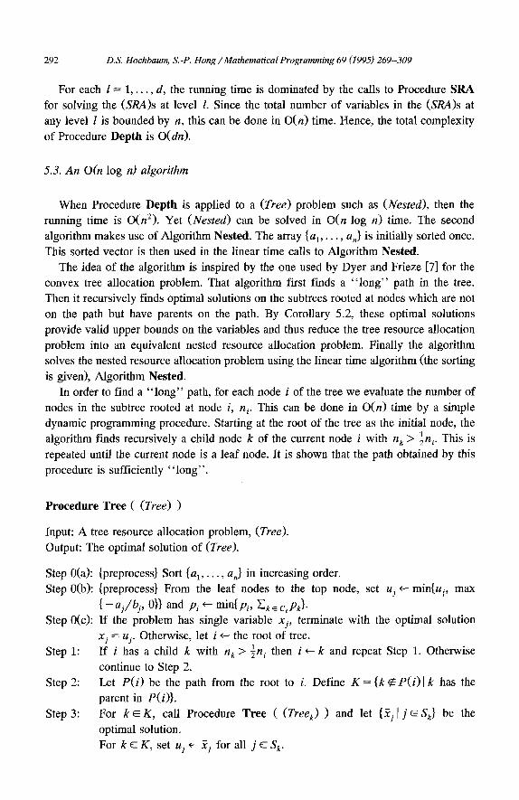
5.3. An O(n log n) algorithm
When Procedure Depth is applied to a (Tree) problem such as (Nested), then the running time is O(n2). Yet (Nested) can be solved in O(n log n) time. The second algorithm makes use of Algorithm Nested. The array {al , . . . , a n} is initially sorted once. This sorted vector is then used in the linear time calls to Algorithm Nested.
The idea of the algorithm is inspired by the one used by Dyer and Frieze [7] for the convex tree allocation problem. That algorithm first finds a " long" path in the tree. Then it recursively finds optimal solutions on the subtrees rooted at nodes which are not on the path but have patents on the path. By Corollary 5.2, these optimal solutions provide valid upper bounds on the variables and thus reduce the tree resource allocation problem into an equivalent nested resource allocation problem. Finally the algorithm solves the nested resource allocation problem using the linear time algorithm (the sorting is given), Algorithm Nested.
In order to find a " long" path, for each hode i of the tree we evaluate the number of nodes in the subtree rooted at node i, n i. This can be done in O(n) time by a simple dynamic programming procedure. Starting at the root of the tree as the initial node, the
1 algorithm finds recursively a child node k of the current node i with n« > 7n i. This is repeated until the current node is a leaf node. It is shown that the path obtained by this procedure is sufficiently " long" .
Procedure Tree ( ( T r e e ) )
Input: A tree resource allocation problem, (Tree). Output: The optimal solution of (Tree).
Step 0(a): {preprocess} Sort { a 1 . . . . . a n} in increasing order. Step 0(b): {preprocess} From the leaf nodes to the top node, set uj ~-min{u j, max
{ - aJby, 0}} and Pi ~ min{p/, Ek ~ ciPk}. Step 0(c): If the problem has single variable xy, terminate with the optimal solution
xy = uj. Otherwise, let i ~ the root of tree. 1 Step 1: If i has a child k with n k > ~n i then i <-k and repeat Step 1. Otherwise
continue to Step 2. Step 2: Let P(i) be the path from the root to i. Define K = {k q~P(i)[k has the
parent in P(i)}. Step 3: For k ~ K , call Procedure Tree ( (Tree k) ) and let {~ j [ j ~ S e} be the
optimal solution. For k ~ K, set uy <-- ~j for all j ~ Sk.
Step 4: Let (Nested) be the nested problem defined by the constraints corresponding to the nodes in P(i) and the updated upper bounds in Step 3. Solve (Nested) by Algorithm Nested.
Theorem 5.4. Procedure Tree is correct and solves the problem in O(n log n) steps.
Proof. Step 1 finds the " long" path in tree in O(n) time. Step 2 identifies the roots of subproblems appended in the path, which also can be done in O(n) time. Step 3 solves the subproblems by recursive calls to Procedure Tree. Denote by C(n) the complexity of Procedure Tree applied to the problem with n variables, then the total running time is Ek ~ KC(nk) time. O(n) time is required to update all upper bounds in Step 3. After Step 3, we obtain a nested resource allocation problem on n variables. Finally, Algorithm Nested solves this nested problem in O(n) time using the presorted data.
The validity of the algorithm follows from Corollary 5.2 which ensures the equiva- lence of the original tree resource allocation problem and the nested resource allocation problem obtained in Step 3. Since every step except the recursive calls can be done in linear time, the total complexity is given by,
C(n) <<. ~_~ C(nk) +an, (5.3) k~K
for some constant A. Assume inductively that C(m) <~ Dm log m for all m < n for some constant D. From (5.3),
1 1 C(n) <~ ~_ù Dn k log n k + A n ~ D log Tn ~_~ n k + A n = D n log Tn+An. k~K k~K
Taking D >_-A/log 2, we get C(n) ~Dn log n. By induction the stated complexity follows. []
6. A strongly polynomiai algorithm for (Network)
Fujishige [9] showed how to solve for a lexicographically optimal base of a polymatroid using n calls to an oracle identifying a maximal independent vector of a polymatroid. Fujishige notes explicitly, that this algorithm is applicable for solving the problem (Network) with strictly convex and homogeneous (that is, without the linear terms - a« = 0 for all k) cost function. As is easily established, the same algorithm applies with a minor modification also to the nonhomogeneous case, including linear terms, for a strictly convex cost function. Such algorithm requires in this case n calls to a procedure solving the maximum flow problem.
Gallo, Grigoriadis and Tarjan [12], in their significant work on parametric maximum flow problem, noted that their algorithm is applicable to the lexicographically optimal flow problem, and the problem is solvable in the running time of a single application of the preflow algorithm of Goldberg and Tarjan [13]. The lexicographically optimal flow also provides an immediate solution to (Network) if the cost function is strictly convex
294 D.S. Hochbaum, S.-P. Hong /Mathematical Programming 69 (1995) 269-309
and homogeneous. Unlike Fujishige's algorithm, the lexicographically optimal flow algorithm of [12] does not extend to the nonhomogeneous case without change in the running time. This is because, as explained later, their algorithm requires that the parametric capacities are linear in the parameter, while for (Network) with nonhomoge- neous cost these capacities are piecewise linear. The purpose of this section is to devise and validate a lexicographically optimal flow algorithm that runs in the same time as a single application of the preflow algorithm, in the presence of piecewise linear paramet-
ric capacities. This algorithm is shown to be applicable to solving (Network) with nonstrictly convex and nonhomogeneous cost in the running time of a single application of the preflow algorithm.
It is also shown that the algorithm of [12] for finding all breakpoints of the cut capacity of a parametric flow network with linear parametric capacities has invalid initialization procedure. We propose an alternative valid initialization procedure that corrects for the flaw in that algorithm.
The equivalence of (Network) and the lexicographically optimal flow problem is discussed in Subsection 6.1. In Subsection 6.2, we show how to formulate a parametric flow problem to solve the lexicographically optimal flow problem. Subsections 6.3 and 6.4 contain the properties of the parametric flow problem which are used to prove the validity of the algorithm presented in Subsections 6.5 and 6.6. In Subsections 6.5 and 6.6, we present the algorithm, based on the algorithms in [12], that solves the lexicographically optimal flow problem.
6.1. Lexicographically optimal flow problem
Let G be the multiple sink flow network on which problem (Network) is defined (as in Subsection 2.1, (5)). The following observations and assumptions simplify the
problem: The optimal solution x satisfies x k <~--ak/b ~, hence we may set u k min{u k, - ak/bk}; As the maximum flow value may not exceed the capacities of the arcs adjacent to the sink, B ~ min{B, Etk ~ ruk}, and it is assumed without loss of generality that B is the maximum flow value. To ensure that, we add an additional arc going into the sink s with capacity equal to B and cost zero. The flow on that arc is then one component of the out-flow vector.
Let the set of sinks be T = {t» t » . . . , t,,} and x i the flow from sink ti to t. Then the
network resource allocation problem is rewritten as:
(Network) min ~bk x k + ak x k k = l
s.t. x = ( x 1, x a . . . . . x~) is the out-flow vector of a
maximum flow f of G.
The corresponding lexicographically optimal flow problem is defined:
(Lexico) Find a maximum flow f which lexicographically maximizes
The following theorem due to Fujishige [10] and an additional observation stated as Lemma 6.2 establishes the equivalence of (Network) and (Lexico).
Theorem 6.1. Let r be a submodular function defined on a distributive lattice A of subsets of E, a finite set, and let {gk(Xk)[ k ~ E} be differentiable convex functions. Consider the following optimization problem (which is similar to (GAP) defined in Section 1 except that the constraint on the set E is equality and there are no nonnegativity constraints)
(GAP') min ~ gk(xk) k~E
E xk = r ( E ) k~E
~_,xk<~r(A), A ~ A . kEA
Then x is an optimal solution of (GAP') if and only if x lexicographically maximizes the vector whose kth component is the kth smallest element of the vector of derivatives, {g~(xk) I k ~ E}.
Lemma 6.2. Let r be defined on the lattice of all subsets of E. Assume that r is monotone, i.e. for every pair of subsets A, B GE with A GB we haue r (A) <,% r(B). Then every feasible solution of (GAP') is nonnegative.
Proof. Suppose that ~ is a feasible solution of (GAP') with Xp < 0 for some p ~ E. Then,
r ( E - { p } ) > ~ ~,, Y c k = r ( E ) - 2 p > r ( E ) > ~ r ( E - { p } ) , k ~ E - { p )
which is a contradiction. []
Theorem 6.1 has an analogue for the network resource allocation problem.
Theorem 6.3. x* = {x; It k ~ T} is an optimal solution of (Network) if and only if x* is the out-flow vector of a solution f of (Lexico).
Proofi For all S _ T, define r(S) to be the value of maximum flow achievable through the subset of sinks, S. In particular, r ( T ) = B, the maximum flow value of G. It is known (see e.g. [9]) that r is a submodular function and (Network) can be written as
r is a monotone function defined on the set of all subsets of T. So by Lemma 6.2, the nonnegativity constraints, (iii) can be relaxed from (P(6.1)) without ehanging the solution. Thus our theorem directly follows from Theorem 6.1. []
For the case when a h = 0 and b h > 0 for all k = 1 . . . . , n, Fujishige [9] developed a strongly polynomial algorithm which solves (Lexico) in the time required to solve at most 2 n - 1 maximum flow problems on G. It can be easily shown that the same algorithm can be used to solve the general case in which a 4= 0 in the same running time
by the translation, Yh = x h - ab/bh of the submodular polyhedron of (P(6.1)) as the translation preserves the submodularity. This running time exceeds the running time established here by a factor of O(n).
6.2. The parametric flow problem
In order to solve the problem (Lexico), we consider the network G with parametric
capacities ck(A) assigned to eaeh arc (te, t) for k = 1 . . . . , n, with co(A) = max{0, (A - a«)/b h} defined for A >~ min{ab I k = 1 , . . , n}. As shown in the following subsection, from the breakpoints of the parametric flow problem defined on G with the parametric capacities, one can construct a solution of (Lexico) and hence a solution of (Network).
The parametric capacities functions ch(A) are monotone increasing in A, where the parametric algorithm of [12] which we use requires that the capaeity functions at the sink are nonincreasing, and at the source they are nondecreasing. To this end we reintroduce the problem with the reversed roles of source and sinks.
(Lexico') Find a maximum flow f on G which lexieographically
maximizes the n-component vector whose kth element is the
kth smallest element of {bkx h + a h I sh ~ S}.
In the reversed network, G, we have a sink s and ares (s, s h) for k = 1 . . . . . n (each
s h corresponds to a t h in G.) Each arc (s, s h) of 6 is assigned the parametric capacity ch(A). Denote this parametric flow network by G(A); so G(Ä) with some fixed value
A = Ä stands for the network 6 with capacity ck(Ä) on each arc (s, s k) and 6 ( ~ ) is 6 with each arc (s, s k) assigned infinite capacity. For an s - t cut (X, X) of G, ca(X, X ) denotes the capacity of (X, ,~) in G(A). Let K(A) be the capacity of minimum s - t cut
of 6(,~). In order to establish the validity of the algorithm several important properties of G(A)
are considered first.
6.3. Properties of G(A)
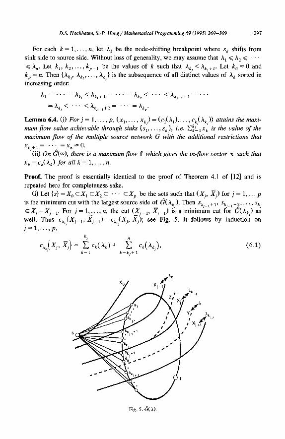
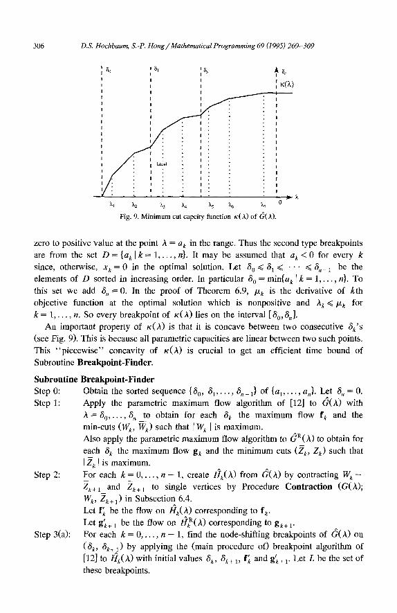
The minimum cut capacity function K(A), as shown in Subsection 6.6, is a monotone nondecreasing piecewise linear function. Ler the breakpoint of K(A) be the value of A where the slope of K(A) changes. At certain breakpoints, some nodes of 6 shift from the sink side to source side as A increases; we call such breakpoints node-shifling breakpoints.
For each k = 1 , . . , n, let A k be the node-shifting breakpoint where s k shifts from sink side to source side. Without loss of generality, we may assume that A 1 ~< A 2 ~< • • • <~ Aù. Let kl , k 2 , . . , kp_ 1 be the values of k such that Akj < Akj+ 1. Let k o = 0 and
kp = n. Then {Akt, Ak2 . . . . . A«p} is the subsequence of all distinct values of A k sorted in increasing order:
A1 . . . . . A k 1 < l~k I + 1 . . . . . A k 2 < " ° " < l~kj_ 1 + 1 . . . .
= A k t < . . . <Akt,_1+1 . . . . . Akp.
L e m m a 6.4. (i) For j = 1 . . . . . p , ( x 1 . . . . . x k ) = (cl(A 1) . . . . . c « ( A k )) attains the maxi-
mum f low value achievable through sinks {sl . . . . . sk), i.e. E ~ ~ l x k is the value o f the maximum f low of the multiple source network G with the additional restrictions that
X k j + l . . . . . X n ~ O .
(ii) On G(~), there is a maximum f low f which gives the in-flow vector x such that
x k = ck(A k) for all k = 1 , . . , n.
Proof. The proof is essentially identical to the proof of Theorem 4.1 of [12] and is repeated here for completeness sake.
(i) Let {s} = X 0 c X 1 c X 2 c . . . c X p be the sets such that (Xi, Xj) for j = 1 , . . p
is the minimum cut with the largest source side o_f G(Akt). Then ski - 1+ 1, Ski_l+2 . . . . , Sk i ~ X j - X j _ 1. For j = 1 , . . , n , the cut (_Xj_» Xj_ 1) is a minimum cut for G(Ak) as
well. Thus C xk(Xj_I , Xj_ 1)= cxk(Xj, Xj); see Fig. 5. It follows by induction on j = l . . . . . p,
kj
c%(Xj , X j ) = ~ c / ( A k ) + f i Ck(Akj), (6 .1) k = l k = k j + l
Which, in turn, implies (i). (ii) Consider the maximum flows, f~, f2 . . . . , fp generated by the parametric flow
algorithm of [12] for the successive parameter A values Akt, Ach, . . . . Ak. When the parametric maximum flow algorithm is restarted with new value A~j of A, the flow on each arc (s, s k) with k ~ {ky_ 1 + 1, ky_ 1 + 2 , . . , n} is first increased frorn ck(A~j_~) to ck(Ak~). This additional flow will reach the sink t, because of (6.1) and the fact that (Xj, Xj) is the minimum cut of G(Akj). By repeating the argument inductively on j = 1 . . . . , p, we have xk= ck(A k) for k = 1 . . . . . n. In particular fp is the desired flow.
[]
Remark 1. The proof holds for any type of parametric capacities once they satisfy the monotonicity assumption and the range of A begins at the point where all parametric capacities are zero.
Remark 2. In the proof of Theorem 4.1 of [12], the cut (Xj, Xy) is claimed to be not only the minimum s - t cut but also the smallest source side of minimum s - t cut of G(A«j+I). This is false even in the simpler case where the parametric capacities are linear functions without constant terms: if there is alternate cut (Z, Z) such that sl . . . . . ski ~ Z, c(Z - {s}, Z) = c(Xj - {s}, Xj) and Z is properly contained in Xj (see Fig. 5), then (Z, Z) is also a minimum s - t cut of G(Ak~+l), and such an example is not hard to construct. Consequently, the breakpoint algorithm as currently stated in [12] is invalid, since "contracted" subsets of vertices in the initialization step are not necessar- ily disjoint. In Subsection 6.4, we define a new method of "contracting" a pair of subsets of vertices which are not disjoint but still possess the property required for the breakpoint algorithm.
Lemma 6.5. Let ~ be a value such that Akj < 6 < A~j+ 1 for some 1 <~ j <~ p - 1. Then ( Xj, Y,i) is the minimum s - t cut with largest source side of G(6).
Proof. Let (Y, Y) be the minimum s - t cut of G(B) such that [YI is maximum. Then since A,i </~, we have Xj ~ Y. Our claim is that Xj = Y. So assume the contrary: assume that Y properly contains Xj. Then Y must contain an element Sq ~{skj+l, ski+2, . . , ski+) with %(6) > 0 (see Fig. 5) since otherwise
c ( Y - { s } , Y ) = c ( X y - { s } , L ) , (6.3)
and hence cak(Y, Y ) = cAk(Xj, Xj). This implies that (Y, Y) is a minimum cut of ^ , J . J . .
G(Ak). But it contradlcts tlie maxlmahty of [Xy [. This however means that 6 is a breakpoint of K(A) at which the node Sq shifts from
the sink side to source side. But it is not possible since Akj+x is the smallest breakpoint larger than 3% and Akj < 6 < Aki+l. So Xj = Y. []
Consider now the reversed parametric network Gg(A) of G(A), i.e. the parametric network obtained from G(A) by reversing the directions of all arcs, considering the sources as sinks and sink as source while maintaining the same capacities (Fig. 6). When the parametric maximum flow algorithm of [12] is applied to Gg(A), the parameter A is replaced by - / x in order to satisfy the monotonicity requirement. For j = p, p - 1 . . . . ,1,
the algorithm finds the minimum cut with the largest source side (X}, X)) (in the reversed network) for the breakpoint --Akj; see Fig. 6. for -A«j+. An argument analogous to the one in the proof of Lemma 6.5 implies that if Akj < 6 < Akj+~ (so --Akj+~ < --6 < --Akj), then (.,~~+ 1, X~+ 1) is the minimum cut with the largest source side for tz = - õ in the reversed network.
Corollary 6.6. Let 6 be a value such that A~j < 6 < Akj+l for some 1 <~ j <~ p - 1. Then
(X~+ 1, X}+ 1) is the minimum s - t cut with smallest source side o f G( $ ) where ( X) , X~ )
denotes the minimum s - t cut with smallest source side o f G(A~j) for k = 1, 2 . . . . . n.
The following lemma is also needed for the algorithms in subsequent subsections.
Lemma 6.7. (i) X~+ 1 c X j but, (il) X~+ 1 is not contained in X j_ 1.
Proof. (i) follows from the fact that (Xj, .Yj) is a minimum cut of G(Akj+l) as mentioned in the proof of Lemma 6.4.
To prove (ii), assume X~+ 1 c_Xj_ 1. Then in G(Ak,+l), for every k ~ {kj_ 1 + 1, kj_ 1 + 2 . . . . . kj}, the arc (s, s k) is saturated with the flow equal to ck(A~ +1). But ck(Akj+l) >~ ck(Ak~) for every k. Furthermore, there is at least one index q ~ tkj_ 1 + 1, kj 1 +
2 . . . . , kj} such that Cq(l~kj) > 0 since otherwise (Xj, Xj) would not have been an s - t minimum cut of G(Ak). This implies that cù(A k ) > c_(A k ).
Thus (6.1)implies ihat for I + {1, 2 . . . . . kj_ li+~ (Xj+ 1 j {s}),
k~l
But in G(Akj_I) for each k e l , the flow ck(A k) on the arc (s, s k) can reach the sink t through the cut (X~+ 1 - {s}, - ' X~+ 1) of G. Hence,
cœ(X;+I--{S}, ~tj+l) 9 E Ck(J~k), k~l
which is a contradiction. []
6.4. The contraction of G(A)
Let 6 and A be different values of A with 6 < A. Assume that all parametric capacities are linear functions of A on the closed interval [6, A] (but not necessarily outside the interval). Let f(g) be a maximum flow and (W, W) ((Z, Z), respectively) be the corresponding minimum cut with the largest source side of G(6) (GR(A), respec- tively).
The purpose of this subsection is to show that the node-shifting breakpoints of G(A) on the open interval (6, A) can be found by the breakpoint algorithm of [12]. We first present a modified initialization procedure to correct for the flaw addressed in Remark 2.
The initialization procedure of the algorithm contracts W and Z into source and sink respectively, where by the contraction of a subset of vertices we mean shrinking of the vertices of the set into a single vertex, eliminating loops and combining arcs by adding their capacities. This contraction procedure is to achieve the property that
(*) in the contracted network, the s - t cut with the trivial source side {s} (sink side {t}) is the unique cut which corresponds to a minimum s - t cut of G(ô) (G(A), respectively),
where the correspondence is the one obtained by expanding the contracted vertex set. However, as pointed out in the Remark 2 of the previous subsection, W and Z are not
necessarily disjoint and the contraction procedure as proposed in [12] is invalid. The following preliminary lemma is needed to establish the modified initialization
procedure. Its proof follows directly from Lemma 6.5, Corollary 6.6 and Lemma 6.7.
Lemma 6.8. G(A) has node-shifting breakpoint on the open interval (6, A) if and only if W does not include Z; or equivalently, W U Z is a proper subset of the vertex set of G( A).
Procedure Contraction(G(A); W, 2)
Step 1" For every source s c E W A 2, delete the arc (s, s c) from G(A). Step 2: Contract W - Z and 2 into single vertices. Call this contracted parametric
Let f' be the flow G(~ a)(A) which corresponds to f of G(A). Let g' be the flow of G~, a)(h) which corresponds to g of GR(A). If G(~, a)(A) has at least three vertices, continue to the (main procedure) of the breakpoint algorithm with initial values f', g', 6 and zl; otherwise G(A) has no node-shifting breakpoints on (6, A); stop.
Suppose a source Sq ~ W N Z in Step 1 (see Fig. 7). Since 6 < A, c~(W, W ) = c s (W
N Z, W N Z). So Xq = 0 in f. Once Sq is in the source side of an s - t minimum cut of G(6), for every h >~ 6, there is an s - t minimum cut of G(h) in which Sq is in the source side. Thus for every h >~ 6_, Xq = 0 in the maximum flow of G(,~). So we can delete (s, %) for every S q ~ W N Z without changing the breakpoints.
Consider Step 2 of the contraction. W is maximum and W n Z is shrunk into the sink. Hence, in the contracted network, G(a, ,~)(h) where W - Z is shrunk into source, the s - t
cut with the trivial source side is the unique cut corresponding to a minimum s - t cut of G(6) (see Fig. 7). Also by the maximality of Z, it is elear that the s - t cut of G(~, a)()0 with the trivial sink side is the unique cut corresponding to an s - t minimum cut of ~(A). Thus (*) is achieved in this contraction procedure.
By Lemma 6.8, G(,~) has node-shifting breakpoints on (6, A) if and only if W U Z is a proper subset of the vertex set of G(h); which means G~~, ,a)(,~) has more than two vertices. Thus if G(~, a)(A) has only two vertices, source and sink, then we conclude that the original problem has no breakpoints in (6, A) and terminate. Otherwise we apply the breakpoint algorithm of [12] to G(~, A)(h).
The details of the breakpoint algorithm of [12] are now briefly sketched: The (main procedure of the) breakpoint algorithm of [12] starts with a pair of parametric flow networks: G(~, a)(h) with initial preflow f' and G(~, a)(A) with initial preflow g'. Under the assumption that all parametric capacities are linear on [6, A], the minimum cut capacity is a piecewise linear concave function of h on [ 6, A]. Thus the next guess ~ of a node-shifting breakpoint on (6, A) can be calculated as the intersection of two tangent lines determined by the leflmost and the rightmost line segments of the (piecewise linear concave) minimum cut capacity function (restricted on [6, A]). The algorithm deter- mines whether ~? is a node-shifting breakpoint by calculating the tangent lines deter- mined by the s - t minimum cuts with the largest source side and the smallest source side
for A = r/; if they do not coincide then ~/ is indeed a node-shifting breakpoint. The algorithm repeats this procedure on the next search intervals [6, r/] and [r/, A]. To obtain efficient time bound, in the current interval [6, A] the algorithm finds a maximum flow (and a minimum cut) for A = 7/by concurrent invocation of the preflow algorithm, for both G(~, a)(h) with initial preflow f' and G(~, a)(A) with initial preflow g'. By doing this the algorithm can "balance" the numbers of nodes between the source side and the sink side of the minimum cuts considered in the subsequent search intervals. The algorithm finds the node-shifting breakpoints on (6, A) in O(N'M' log(N'2/M')) steps, where M' and N' are respectively the numbers of arcs and nodes of G(~, a)(h).
6.5. The main algorithm
When a = 0, the main algorithm is identical to the algorithm in Subsection 4.1 of [12] with the exception of using the modified subroutine, Subroutine Breakpoint-Finder for finding the node-shifting breakpoints of the minimum cut capacity function K(A), of d(,O.
Algorithm Lexico-Finder
Step 0:
Step 1:
Step 2:
Step 3:
Step 4:
Augment the network G with a dummy source s and the arcs (s, s k) for k = l , . . . , n . Call this augmented network G. Assign the parametric capacity ck(A)=rain{0, ( A - ak)/b k} to each arc (s, s k) of G. Denote the parametric flow network by G(A). Call Subroutine Breakpoint-Finder to find the node-shifting breakpoints of K(A) for A ~> min{ak I k = 1 . . . . . n} For each source s~, k = 1 , . . . , n, find the node-shifting breakpoint A k at which s k shifts from sink side to source side of a minimum s - t cut of G(A k) as A increases. Assign the capacity ck(A k) to each arc (s, s~) of G. Find a maximum flow f on the network with these upper bounds. Output the in-flow vector x of f as the optimal solution of (Lexico').
Subroutine Breakpoint-Finder is given in the next subsection. In the following theorem, we prove the validity of the main algorithm under the assumption that Subroutine Breakpoint-Finder correctly finds the node-shifting breakpoints of K(A).
Theorem 6.9. Algorithm Lexico-Finder is correct: the maximum flow f obtained in Step 4 gives the in-flow vector x which is the optimal solution of the problem (Lexico').
Proof. Consider the breakpoints of Step 3, A1,..., A n. Without loss of generality, we may assume that A1 ~ A 2 ~< • • • ~< A n. Let k 1, k2 , . . . , kp_~ be the values of k such that
Akj < Akj+l. Let k 0 = 0 and kp = n. Then {Akl, Ak2 . . . . . Akp} is the subsequence of all
distinct values sorted in increasing order: Also let f be the maximum flow obtained in
Step 4. By Lemma 6.4, the in-flow vector x of f satisfies x k = ck(A k) for all k = 1 . . . . , n
and:
Faet 1. For j = 1 . . . . . p , ( x I . . . . . Xkj ) = (cl(A 1) . . . . . ckj(Akj)) attains the maximum flow
value achievable through sinks {s 1 . . . . . sk), i.e. E~~lx~ is the value of the maximum
flow of the multiple source network G with the additional restrictions that xkj + 1 . . . .
x n = 0 .
From the definition of ck(A):
ck(Ak)=((O A~-ak) /bk ififAk>~ak'A k < a k.
Define ]&k = max{Ak, ak}. Then we have:
Fact 2. ck(A k) = ck(]&k) = ( ]&k -- ak)/bk for all k = 1 . . . . . n.
Fact 3. {A k ] k = 1 . . . . . n} and { ]&k I k = 1 , . . , n} have the identical elements except for
k ' s such that A k < ]&k and ck(A k) = ck(]&k) = 0.
Let o- be the permutation of {1 , . . , n} such that ]&«(a~ ~< ]&«¢2) ~< " " " ~< ]&teù). Let
il, i 2 , . . , iq_ 1 be the values of i such that ].Lo.(ij)< ].Zo_(/j+l). Let i 0 = 0 and iq=n. Then { ]&«~q~, ]&«~i2) . . . . . ]&«<iq~} is the set of all the distinct values in increasing order:
B o ' ( 1 ) . . . . . J[~o(i l) < ] & o ' ( i l + i ) . . . . . ]&o'(i2) < " " " < ] & o ' ( i j - l + l )
. . . . . ]&o ' ( i j ) < " " " < ] & o ' ( i q _ l + l ) . . . . . ]&tr( iq)"
For a fixed j = 1 . . . . . q, let j* denote the maximum value such that Ak~ * ~< ]&«~i?,
then since A~ ~< ]&k for all k = 1 , . . , n we have:
So rar we have proved that the maximum flow f yields the in-flow vector x such that for each j = 1 . . . . . q:
Fact 5 . (Xo-(1) . . . . . Xo-(ij)) --" ( ( /&o- ( l ) - ao-(1))/bo-(1) . . . . . (/&(r(i]) - ao'(ij))//bcr(ij)) is the in-flow sub-vector attaining maximum value achievable through the sinks
{So-(1 ) . . . . . SŒ(i])}"
Fact 6. /&o-(l) ~/&o-(2) ~ " " " ~/&o-(n) and/&«(i0, /&o-(i2),'",/&cr(iq) is the subsequence of all distinct values sorted in increasing order.
b(r (1) x ; ( 1 )
and from (Fact
bù(t) x;(,) Therefore,
It is shown by induction on j = 1 . . . . . q, using (Fact 5) and (Fact 6) that x is the solution of (Lexico') with lexicographically maximized vector (/&«(1), /&«(2),..,/&«(n)). (Alternatively it follows directly from Theorem 9.1 of [16] which is stated in more general terms.)
First, by (Fact 5), (x«o) . . . . . Xo-( i l ) ) = ( ( /&o.(1) - - ao_(1))//bo.(1 ) . . . . . (/&o_(il)--ao.(il))// be(il )) is the in-flow sub-vector attaining maximum value achievable through the sinks {s«o ) . . . . . sc(q)}. So the in-flow vector y of any maximum flow of G satisfies
Y«(~) ~< X°'(1) ' " " " ' YŒ(/1) ~ X°'(il)"
Hence,
b«(1)Y«(1) + acr(1) ~</&o-(l) . . . . , bo'(il)Yo-(il) -[- a g ( i l ) • ]-'~o-(/1). (6.4)
(6.6) and (6.7) imply that x' is a worse solution than x, which is a contradiction. Thus we conclude that the in-flow vector x of f of Step 4 yields the optimal value
(/&co), /&«(2), - . , /&«(n)) to the problem (Lexico'). []
The complexity of the main algorithm, Algorithm Lexico-Finder, excluding Step 2, is the same as the complexity of the maximum flow problem on G. This is since Step 4 requires the maximum flow problem on G, while Step 1 and Step 3 can be executed in O(n) (where n is the number of sources of G.)
In the following subsection, we describe Subroutine Breakpoint-Finder that is called for in Step 2, which finds the breakpoints of K(A) in the time of a single application of the preflow algorithm. It follows that the complexity of Algorithm Lexieo-Finder is the same as that of the preflow algorithm.
6.6. The breakpoint algorithm
When a = 0, Step 2 of Algorithm Lexico-Finder is executed using the breakpoint algorithm of [12] (discussed in Subsection 6.4) which uses the parametric maximum flow algorithm developed in the same paper. While, the parametric maximum flow algorithm works for any type of parametric capacity function once it satisfies the monotonicity assumption, the breakpoint algorithm requires that parametric capacities are also linear functions. When all parametric capacities are linear, the capacity function K(A) is a piecewise concave function with at most n - 2 breakpoints since at each breakpoint at least one source of G()t) shifts from the sink side to source side of a minimum cut as ~t increases.
In our case, each parametric capacity ck(A) is a piecewise convex linear function with single break point (see Fig. 8). So the minimum cut capacity function K(A) is piecewise linear but not concave in general. The function still has nice properties which allow us to use the breakpoint algorithm of [12] as subroutine in order to solve the problem in the same running time.
The set of breakpoints consists of two types of points (which are not necessarily mutually exclusive). The first type of breakpoints are the node-shifting breakpoints (where some nodes of the network shift from the source side to the sink side of a minimum cut as )t increases). Consequently, the number of node-shifting breakpoints is bounded by the number of nodes in G. The second type of breakpoints are derived from the breakpoints of the parametric capacities, {a k I k = 1 . . . . . n}. Even if we may have the same minimum cut over some range of A, there can be a change in the slope of K(A) if the parametric capacity of an arc (s, s k) in the minimum cut begins to increase from
Fig. 9. Minimum cut capcity function K(A) of G(A).
zero to positive value at the point A = a k in the range. Thus the second type breakpoints are from the set D = {a«[k= 1 . . . . ,n}. It may be assumed that a k < 0 for every k since, otherwise, x~ = 0 in the optimal solution. Let 30 ~< 31 ~ ' ' " ~ 3 n _ 1 be the elements of D sorted in increasing order. In particular 30 = min{a~ [ k = 1 . . . . , n}. To this set we add 3ù = 0. In the proof of Theorem 6.9, /z~ is the derivative of kth objective function at the optimal solution which is nonpositive and h k ~</x~ for k = 1 , . . , n. So every breakpoint of K(A) lies on the interval [30,3n].
An important property of K(A) is that it is concave between two consecutive 3k's (see Fig. 9). This is because all parametric capacities are linear between two such points. This "piecewise" concavity of K(h) is crucial to get an efficient time bound of Subroutine Breakpoint-Finder.
Subroutine Breakpoint-Finder Step 0: Obtain the sorted sequence {30, 31 . . . . . 3ù_ 1} of {ap . . . , aù}. Let 3 n ~--- 0. Step 1: Apply the parametric maximum flow algorithm of [12] to G(h) with
h = 30 . . . . . 3ù to obtain for each 3 k the maximum flow fk and the min-cuts (Wk, W k) such that [W k [ is maximum. Also apply the parametric maximum flow algorithm to GR(h) to obtain for each 3 k the maximum flow gk and the minimum cuts (Zk, Zk) such that [Zkl is maximum.
Step 2: For each k = 0 . . . . , n - 1, create /~k(h) from G(A) by contracting W k - Zk+l and Zk+l to single vertices by Procedure Contraction (G(A); W~, Zk+ 1) in Subsection 6.4. Let f~ be the flow on /4k(A) corresponding to fk.
t ^ R Let gk+l be the flow on H~ (A) corresponding to gk+l. Step 3(a): For each k = 0 . . . . . n - 1, find the node-shifting breakpoints of G(h) on
(3~, 3k+ 1) by applying the (main procedure of) breakpoint algorithm of [12] to/~k(A) with initial values 3k, 3k+ 1, f~ and g~+i. Let L be the set of these breakpoints.
Let L' = L U {8 0, 31 . . . . ,6n}. Sort L' in increasing order. Apply the parametric maximum flow algorithm to G(h) for all A ~ L'. Select all the values at which some nodes shift from the sink side to source side and output them as the node-shifting breakpoints of G(h).
Theorem 6.10. Let G have N nodes and M arcs. Subroutine Breakpoint-Finder finds the node-shifling breakpoints of minimum cut capacity function K(A) of G(A) in O(NM log(NE/M)) steps.
Proof. The validity of Step 1 through 3 follows/rom the arguments of Subsection 6.4 which assert that the node-shifting breakpoints of G(A) on (6 k, 6k+ 1) can be found by applying the breakpoint algorithm of [12] to/~«(A) if all parametric capacities are linear on [6~, 6k+1].
The reason for creating the set L' in Step 3(b), rather than just taking L as the set of all node-shifting breakpoints, is that some of the 6k's can be node-shifting breakpoints as weil. Hence the parametric maximum flow algorithm in Step 4, extract all node-shift- ing breakpoints.
Let A ~ and /~ denote the number of nodes and arcs of G(A) respectively. With this notation, A ? = N + 1 and /14 = M + n. Also let N« and M« be the number of nodes and arcs in /~k(A) for k = 0, 1 , . . , n - 1 respectively.
A
Since the number of parameter values, 3k's, is n ~< N - 2, Step 1 also can be done in O(N/~ log(NE//~t)) steps by applying the parametric maximum flow algorithm of [12] to G(A) and GR(A).
For a contraction procedure in Step 2, we need to determine the edges in the cut defined by the vertex set to be shrunk into a single vertex. This can be done in O(/~) steps by a breadth first search. The running time of other efforts, deleting loops and combining arcs is also bounded by O(/~) using a standard data structure for network representation. Since n contraetions are done and n ~< ]V, Step 2 requires O(5,)N) steps.
By Lemma 6.5, Corollary 6.6 and Lemma 6.7, it follows that eaeh node of G()t) can partieipate in at most a single Hk(A) as an unshrunk hode. Henee ù- 1 _ Ek=0N k - O(ü). The running time of the breakpoint algorithm of [12] for the kth contracted network 6 k is O(NkM k log(N2/Mk)). Let A be the constant coefficient of the running time. Then the total work of Step 3 is:
n - 1 n - 1
A ~_~ NkMk log(NE/Mk)<~A ~_, NkM k log(2]VE/Mk) k = 0 k = 0
n - 1
~<A • NkM log(2]V2/M). k=0
The last inequality follows from the fact that the function f ( x ) = x log(K/x) is increasing in the range 0 < x «. K l4 (where K is a positive constant) and M k <~ ffI <~ 2/V2/4. Since n - 1 __ 2k= 0Nk- O(A?), Step 3 requires O(NM log(N2//~)) steps.
The size of L' is O(A?); hence, again by the parametric maximum flow algorithm, Step 4 ean be done in O(Nk)log(/V2//~)) steps. So the total running time of
Subroutine Breakpo in t -F inde r is O(ATAI log(A~2/&l)). Since A ~ = N + 1, h/l = M + n
and n ~< M, the running time is O(NM log(N2/ (M + n))) which is O(NM log(N2/M)). []
Since the running time of Subroutine Breakpo in t -F inde r is O(NM log(Ne/M)), and the dominant operations in Algorithm Lexieo-Finder are the maximum flow on
and the calls to Subroutine Breakpoin t -F inder , it follows that the network resource allocation problem is solvable in O(NM log(N2/M)) steps.
So rar the objective function has been assumed to be strictly convex, i.e. b k > 0 for all k = 1, 2 . . . . . n. Assume now that the objective function is convex but not strictly convex: hence there is a proper subset U c T such that b k = 0 if s k ~ T - U.
Theorem 6.3 is still valid since it does not assume the strict convexity of the objective function. So to solve (Network) is equivalent to solve (Lexico') which finds a maximum
flow of G lexicographically maximizing the sorted sequence of {bkx k + ak[ s~ ~ T} in increasing order.
I f s k ~ T - U , then bkx k + a k is a constant. So it suffices to consider only the elements of {bkx k + a«l s k ~ U}. That is, if x is an in-flow vector of a maximum flow such that the sorted sequence of {bkx k + a k I sk ~ U} in increasing order is the lexico- graphically maximum among all in-flow vectors, then x is the solution of (Network).
This can be done in the following manner: 1. Augment the network G with the arcs (s, s k) and the parametric capacities ck(A) for
only k ' s such that s k ~ U. Apply Algorithm Lexieo-Finder to obtain a maximum
flow g and the corresponding in-flow vector {Yk I sk ~ U}. 2. Create the residual network Gg of G with respect to the flow g. Augment Gg with
the arcs (s, s~) for s k ~ T - U and find a maximum flow of the network. Let the corresponding in-flow vector be {z~[ s k ~ T - U}.
3. Output the in-flow vector {Yk [ sk ~ U} U {zkl s k ~ T - U} as an optimal solution of (Network). The additional work for the general convex case is to find a maximum flow in the
residual graph Gg. Hence the total running time is the same as that of the strictly convex
case.
7. Concluding remarks
We presented new strongly polynomial algorithms for some special cases of discrete and continuous ¢onvex separable quadratic optimizations over submodular constraints. It seems that further improvement on the complexities of the algorithms developed here is going to be challenging.
As mentioned earlier, every problem considered in this paper is a special case of the minimum quadratic cost network flow problem; costs are associated only to the flows on the arcs emanating into the sink of the network. This observation naturally leads us to the important open question of the strong polynomiality of (general) minimum quadratic cost network flow problem. This problem seems to be very challenging. Even if the
number of arcs with quadratic cost is fixed, the question still remains open.
[1] R. Baldick and F.F. Wu, "Efficient integer optimization algorithms for optimal coordination of capacitators and regulators," IEEE Transactions on Power Systems 5 (1990) 805-812.
[2] M.J. Best and R.Y. Tan, "An O(n 2 log n) strongly polynomial algorithm for quadratic program with two equations and lower and upper bounds," Research Report CORR 90-04, Department of Combinatorics and Optimization, University of Waterloo (1990).
[3] M. Blum, R.W. Floyd, V.R. Pratt, R.L. Rivest and R.E. Tarjan, "Time bounds for selection," Journal of Computer and Systems Sciences 7 (1972) 448-461.
[4] P. Brucker, "An O(n) algorithm for quadratic knapsack problems," Operations Research Letters 3 (1984) 163-166.
[5] W. Cook, A.M.H. Gerards, A. Schrijver and E. Tardos, "Sensitivity results in integer linear program- ming," Mathematical Programming 34 (1986) 251-264.
[6] S. Cosares and D.S. Hochbanm, "Strongly polynomial algorithms for the quadratic transportation problem with fixed number of sources,"Mathematics of Operations Research 19(1) (1994) 94-111.
[7] M.E. Dyer and A.M. Frieze, "On an optimization problem with nested constraints," Discrete Applied Mathematics 26 (1990) 159-173.
[8] G.N. Frederickson and D.B. Johnson, "The complexity of selection and ranking in X + Y and matrices with sorted columns," Journal of Computer and Systems Sciences 24 (1982) 197-208.
[9] S. Fujishige, "Lexicographieally optimal base of a polymatroid with respect to a weight vector," Mathematics of Operations Research 5 (1980) 186-196.
[10] S. Fujishige, Submodular Functions and Optimization, Annals of Discrete Mathemafics 47 (North-Hol- land, Amsterdam, 1991).
[11] H.N. Gabow and R.E. Tarjan, " A linear-time algorithm for a speeial case of disjoint set union," Journal of Computer and System Sciences 30 (1985) 209-221.
[12] G. Gallo, M.E. Grigoriadis and R.E. Tarjan, " A fast parametric maximum flow algorithm and applications," SIAM Journal of Computing 18 (1989) 30-55,
[13] A.V. Goldberg and R.E. Tarjan, "A new approach to the maximum flow problem," in: Proceedings of the 18th Annual ACM Symposium on Theory of Computing (1986) pp. 136-146.
[14] F. Granot and J. Skorin-Kapov, "Some proximity and sensitivity results in quadratic integer program- ming," Working Paper No. 1207, University of British Columbia (1986).
[15] F. Granot and J. Skorin-Kapov, "Strongly polynomial solvability of a nonseparable quadratic integer program with applications to toxic waste disposal," Manuscript (1990).
[16] H. Groenevelt, "Two algorithms for maximizing a separable concave function over a polymatroidal feasible region," Technical Report, The Gradnate School of Management, University of Rochester (1985).
[17] D.S. Hochbanm, "On the impossibility of strongly polynomial algorithms for the allocation problem and its extensions," in: Proeeedings of the 1st Integer Programming and Combinatorial Optimization Conference (1990) pp. 261-274; D.S. Hochbaum, "Lower and upper bounds for the allocation problem and other nonlinear optimization problems," Mathematics of Operations Research 19 (1994) 390-409.
[18] D.S. Hochbanm and J.G. Shanthikumar, "Convex separable optimization is not much harder than linear optimization," Journal of ACM 37 (1990) 843-862,
[19] D.S. Hochbanm, R. Shamir and J.G. Shanthikumar, "A polynomial algorithm for an integer quadratic nonseparable transportation problem," Mathematical Programming 55(3) (1992) 359-372.
[20] T. Ibaraki and N. Katoh, Resource Allocation Problems: Algorithmic Approaches (MIT Press, Cam- bridge, MA, 1988).
[21] N. Megiddo and A. Tamir, "Linear time algorithms for some separable quadratic programming problems," Operations Research Letters 13 (1993) 203-211.
[22] G.L. Nemhanser and L.A. Wolsey, lnteger and Combinatorial Optimization (Wiley, New York, 1988). [23] A. Tamir, "A strongly polynomial algorithm for minimum convex separable quadratic cost flow
problems on series-paraUel networks," Mathematical Programming 59 (1993) 117-132. [24] E. Tardos, "A strongly polynomial algorithm to solve eombinatorial linear programs," Operations