Faculty of Bio-science engineering Academic year 2013-2014 Aboveground carbon stock estimation of young reforested areas in Northern Ecuador Rosa Isabel Soria Peñafiel Promotor: Dr. Ir. Hans Verbeeck and Prof. Dr. Ir. Kathy Steppe Tutor: Ir. Elizabeth Kearsley Master’s dissertation submitted in partial fulfillment of the requirements for the degree of Master in Environmental Sanitation
Transcript
Faculty of Bio-science engineering
Academic year 2013-2014
Aboveground carbon stock estimation of young reforested areas in Northern Ecuador
Rosa Isabel Soria Peñafiel
Promotor: Dr. Ir. Hans Verbeeck and Prof. Dr. Ir. Kathy Steppe Tutor: Ir. Elizabeth Kearsley
Master’s dissertation submitted in partial fulfillment of the requirements for the degree of
Master in Environmental Sanitation
COPYRIGHT I
COPYRIGHT The author and promoters give the permission to use this thesis for consultation and to copy parts of it for
personal use. Every other use is subject to the copyright laws, more specifically the source must be
extensively specified when using results from this thesis.
Ghent, june 2014
Prof. dr. ir. Kathy Steppe Dr. ir. Hans Verbeeck ir. Elizabeth Kearsley Rosa Soria Peñafiel
ACKNOWLEDGEMENTS II
ACKNOWLEDGEMENTS Being from an Andean country where I live in a city surrounded by mountains at 2800 (m.a.s.l.), and
then moving to Belgium was something not easy. However, having the opportunity to study in a foreign
land the environmental technics to protect the planet has been without doubt one of the best
experiences in my life. By being witness of the huge differences between my beloved Ecuador and the
old continent I have opened my eyes and changed my mind towards the acknowledgement of the real
richness and the potential that Ecuador’s environment has.
After one year of lessons at the Faculty of Bioscience Engineering, I had the opportunity to go back to
my Ecuador to conduct my thesis field work. When searching for a thesis topic, I with no doubt chose to
work for forest monitoring in Ecuador. I believe that there is nothing better than working to directly
contribute to improve the quality of life of your people and your environment. Although my
contribution could be relatively small, l feel like my work can make a big difference. Together with an
increased theoretical knowledge and my mind full of new ideas I went to Ecuador in the summer of 2013
to develop the field campaign for monitoring reforested areas in the north part of Ecuador. Those were
7 weeks full of experiences, knowing new people and its realities, visiting places that I have never been
before, and discovering abilities at field that I ignored. It was a really hard and intense time but at the
same time it was wonderful. Coming back to Belgium after my field work, I felt I have personally and
academically changed.
I want to thank to all people who contributed to conduct this study, to people of BOS+ and TELENET for
the opportunity of being part of the project, and for the collaboration received from the early stages to
the culmination of the project particularly to Debbie. My gratitude to the people in Ecuador members of
the Mindo Cloudforest Foundation (MCF), who shared their knowledge with me about plantings and
about life; my acknowledgement for Brian, Maura, Blanquita, Martin, Andres and the guys at Suamox. I
am especially grateful to my academic advisors dr. Hans Verbeeck and Elizabeth Kerasley who always
guided and helped me with their opportune suggestions and who were always available for me. Also to
my friend Mauricio who helped me with his knowledge on statistics. And a special recognition to my
friend and mate of life and route Edgardo, who helped me enormously during large part of the field
work because without him I would not be able to complete my task.
To obtaining this master degree collaboration from others was required. Therefore, I want to thank all
people who were part of this incredible experience. To my friends Belencita, Vivi, Juan, Diana, Renzo,
Jane, Daniel, Long, Andre and Laura for all the time shared and their truly friendship. To my cousin
Daniela and her family Amankay and Michael who made me feel that I also have family in Belgium. To all
the staff of the program of Environmental Sanitation, especially to Sylvie, Veerle and Professor Peter
Goethals who were always eager to help me.
Also, I want to thank to my friends of life Xime, Marce, Mauro and Gato who were part of this dream
since the beginning and supported and helped me in all forms. From the day I decided that I wanted to
study in Europe, passing for the work paper for the scholarship, the preparation for the TOEFL, the
ACKNOWLEDGEMENTS III
moment of say goodbye with tears drops in our eyes at the airport, the motivational conversations for
skype in spite of the 6-7 hours of difference. Thank you guys, it is done!
The most important recognition is to my family, my parents Francisco and Ketty who were my guide, my
example and especially my friends during these 28 years of life. I want to thank them because they
always made me feel that I am able of whatever I propose. You made me sensible to the reality and
from that my desire of change the world emerged. Here am I now, changing slowly the world. Also very
especial thanks to my brother and friend Rafa, who is without doubt the smartest and enterprising guy
ever, thank you Rafa for being part of my life, for being an example and being always motivating me to
do more. Thanks to my grandparents Panchita and Humberto who send me prays from heaven. To
Mamita Julia; who is waiting for me at home, thanks for all the blessings and the prays. I am sure that all
your thoughts and positive energy helped me in the hardest moments. And thanks to all the rest of my
family, I am happy for being blessed with this wonderful and big family as we are.
Finally I want to thank to the government of Ecuador trough the National Secretary of Superior
Education Science and Technology (SENESCYT) who believed in my capacities and allowed me to study
abroad. Thanks for investing in preparing people, and for the opportunity to learn from other societies
and realities.
My country is changing, and I am feeling happy of being part of this change.
Rosa Isabel Soria Peñafiel, 27th of May, 2014
ABSTRACT
IV
ABSTRACT
CKNOWLEDGEMENTS In this work the estimation of aboveground carbon stock in two-year-old reforested areas at five
different stratums spread over an altitudinal gradient in the north part of Ecuador was conducted. The
data of 565 trees was analyzed; the estimations were done using allometric equations for young
secondary forest with diameter at breast height (DBH) as predictor variable for biomass. Parallel, basal
area and tree height data were analyzed as an indicator of biomass. As the majority of the monitored
population was smaller than 1.3 m, root collar diameter (RCD) was recorded and corrected to be used in
the allometric models. The correction was performed using the relation DBH=0.46 ± 0.14 RCD obtained
from trees that were high enough to record both parameters. Because of the impossibility of destructive
measurements, it was not possible to state which model performed better. The average between the
three tested models was considered as the best estimate of the state of the plantings. In addition, the
numbers of trees as well as the species present at each stratum were analyzed to determine their
influence on the biomass.
The results based on basal area and tree height observations pointed out stratum 3 as the highest stock
of carbon, while the allometric models pointed stratum 2 as the main stock of carbon with 149.25 kg.ha-
1 ± SD 1.41. High variability in corrected DBH was observed in all strata with exception of stratum 4; the
highest variability was present in stratum 2. Both allometric estimations as well as basal area showed
stratum 1 as the lowest carbon stock with 13.36 kg.ha-1 ± SD 0.24. The difference between allometric
estimation and basal area pattern responded to the presence of some extreme values observed in
stratum 2; these extreme values corresponded to the fast growing Alnus sp. Other fast growing specie,
Inga sp. was identified at stratum 3 as well demonstrating high performance. The presence of slow and
mid successional trees was denoted by the presence of Cedrela montana. A decrease of aboveground
biomass was observed with increasing altitude with exception of stratum 2, which possessed favorable
climatic conditions and the above mentioned fast growing specie.
These results are the first estimation since the plantation in 2012, and will become the baseline of
future monitoring. However the scope of the current analysis is limited as now there is only one
observation available. Re-census observations in the coming years are needed to assess the progress of
the plantings regarding aboveground carbon stock. The development of local allometric models is
recommended for future campaigns.
V
LIST OF TABLES
Table 1: Carbon pools in the major reservoirs on Earth .............................................................................. 5
Table 2: Carbon stock in forest by region.. ................................................................................................... 7
Table 3: Summary of factors observed to explain spatial variation in aboveground biomass in tropical
Table 11: Summary of number of trees per plot and per stratum. ............................................................ 29
Table 12: Report of mortality type. ............................................................................................................ 30
Table 13: Average basal area per stratum. ................................................................................................. 30
Table 14: Average tree height estimations per strata. ............................................................................... 31
Table 15: Aboveground biomass estimations using different allometric models for strata 1 to 5. ........... 35
Table 16: Average estimation of aboveground carbon. ............................................................................ 36
Table 17: Mean aboveground carbon AGC [kg] per specie and per stratum. ............................................ 60
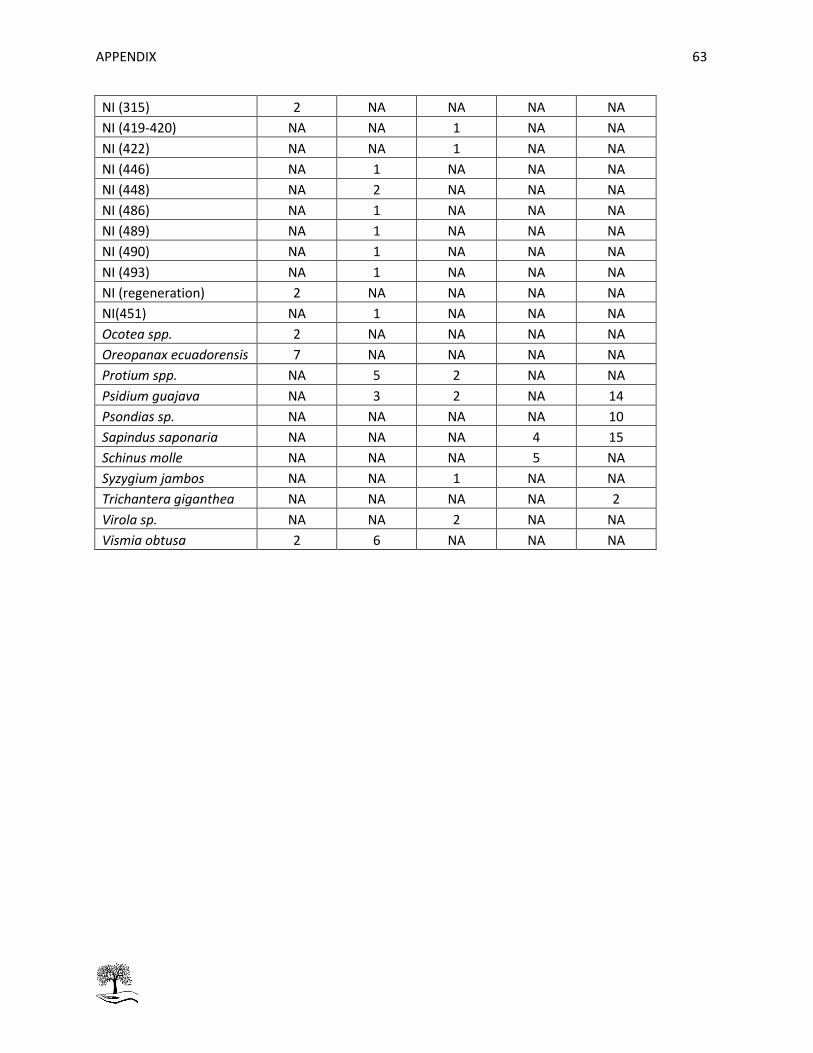
Table 18: Number of trees per specie and per stratum. ............................................................................ 62
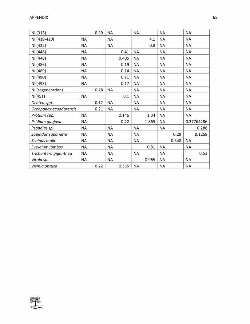
Table 19: Mean height [m] per specie and per stratum. ............................................................................ 64
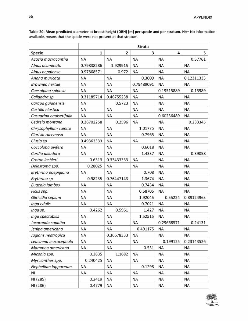
Table 20: Mean predicted diameter at breast height (DBH) [m] per specie and per stratum. .................. 66
VI
LIST OF FIGURES Figure 1: Scheme of global terrestrial carbon uptake. ................................................................................. 6
Figure 2: Representation of the hierarchical nature of the relationships between aboveground biomass
(AGB) and stand and environmental descriptors. ........................................................................................ 9
Figure 3: The error propagation for estimating the ABG of a tropical forest from permanent sampling
Figure 4: Location of the study area, with an overview of each one of the five strata. ............................. 21
Figure 5: Images depicting the panorama between the different stratums. ............................................. 23
Figure 6: Graphical representation of the circular plots for monitoring.. ................................................. 24
Figure 7: Determination of DBH or POM in case of slopes (left) or fallen or leaning trees (right).. ........... 25
Figure 8: Measurement of tree height using an electronic hypsometer.. .................................................. 26
Figure 9: Boxplot of the basal area from the five different planted stratums ........................................... 31
Figure 10: Boxplot of the tree height data from the five different planted stratums ................................ 32
Figure 11: Influence of using RCD in allometric equations designed for DBH. ........................................... 33
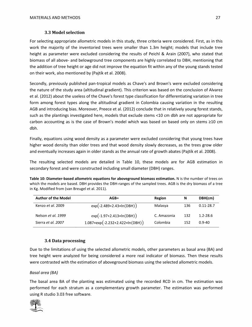
Figure 12: Relations for predicting DBH based on RCD. . ........................................................................... 34
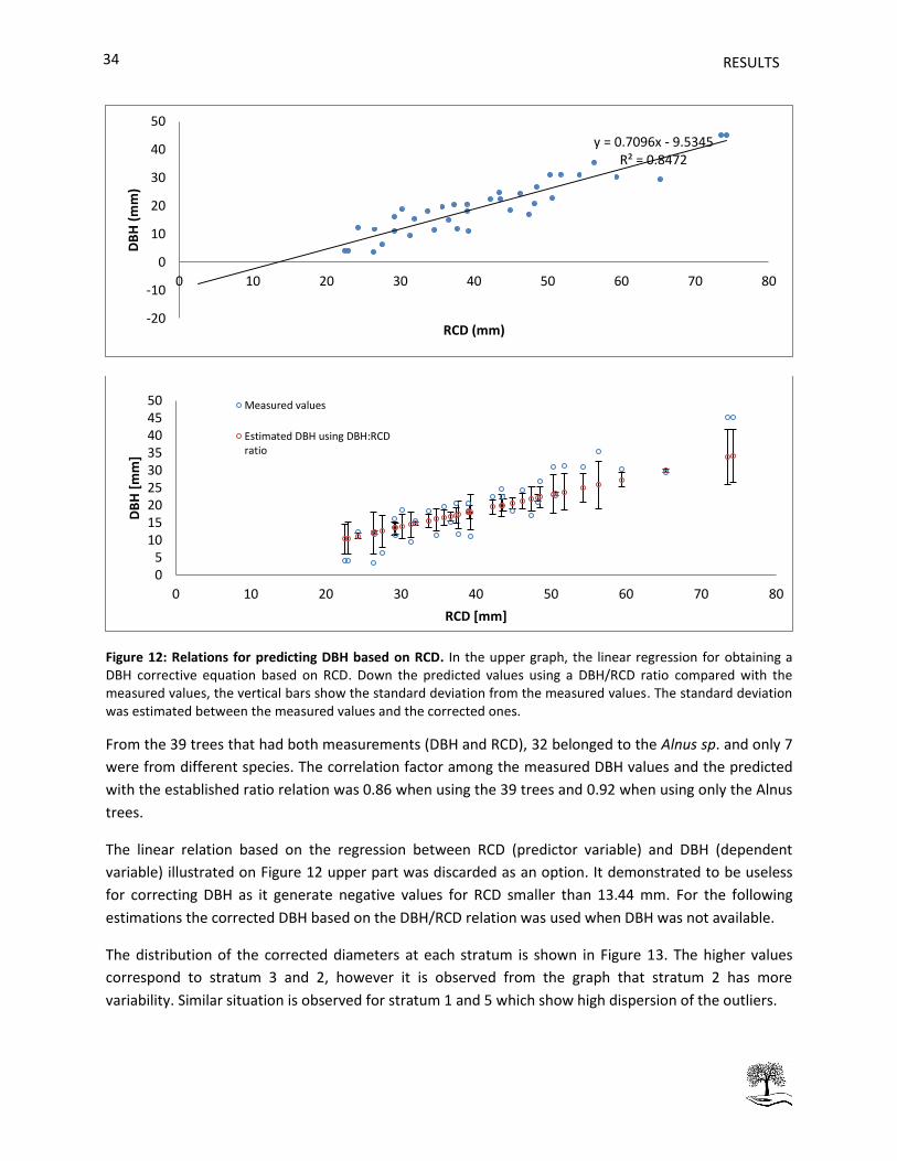
Figure 13: Distribution of the corrected DBH per strata for the complete data set. ................................. 35
Figure 14: Distribution of the aboveground carbon average estimation. .................................................. 36
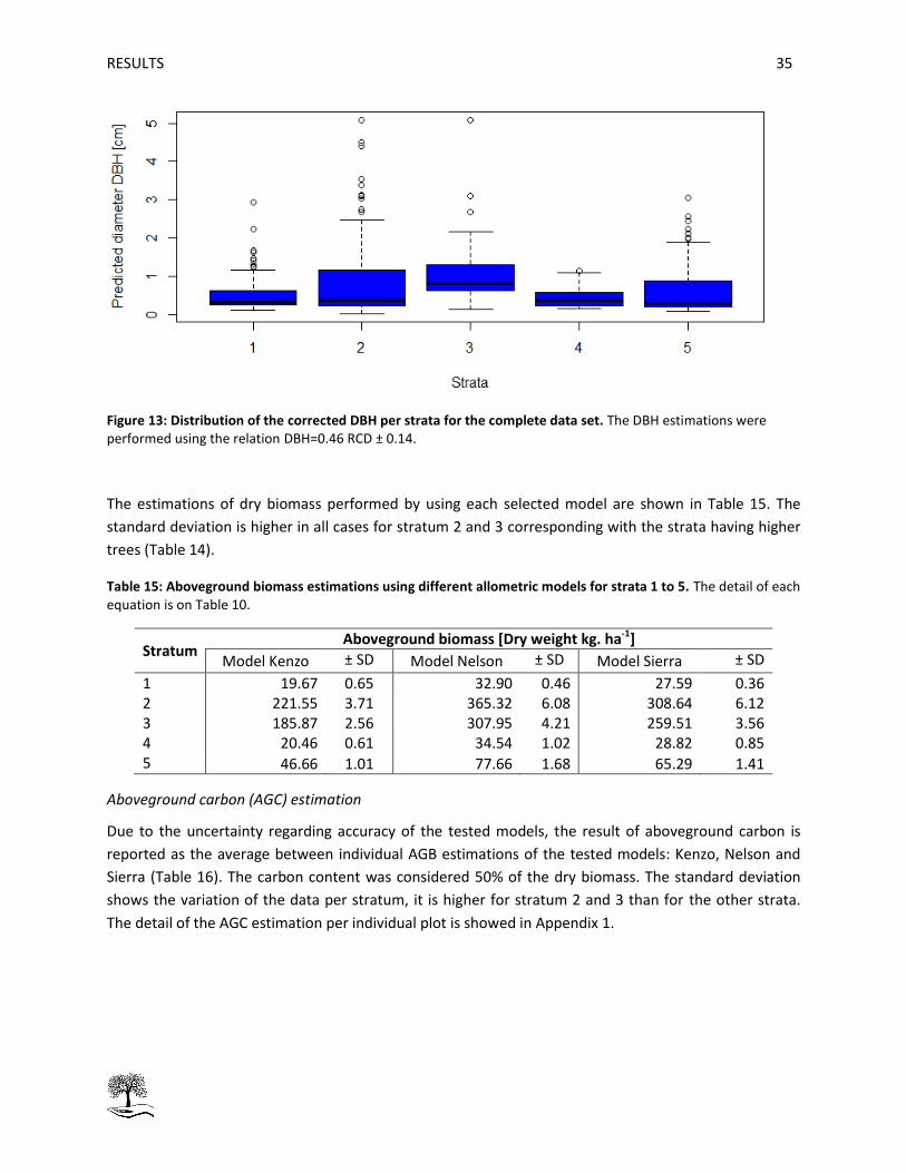
Figure 15: Graph showing the AGC content in the inventoried permanent sampling plots on the
different reforested strata spread over northern Ecuador.. ...................................................................... 37
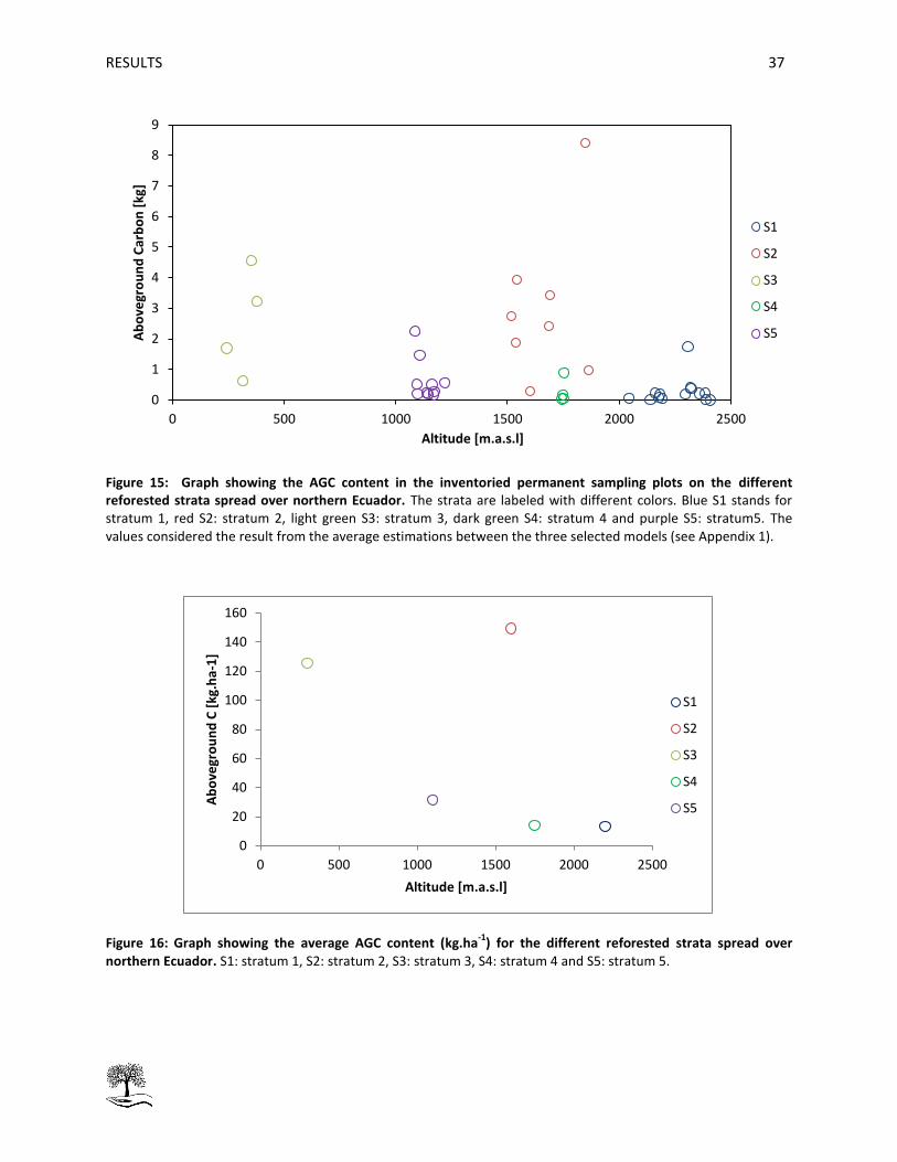
Figure 16: Graph showing the average AGC content (kg.ha-1) for the different reforested strata spread
over northern Ecuador ................................................................................................................................ 37
Figure 17: Relation between aboveground carbon, basal area and tree height. ....................................... 38
Figure 18: Relationship between aboveground biomass and basal area.. ................................................. 39
Figure 19: Tree species and its aboveground carbon stock distribution per strata.. ................................ 40
LIST OF ABREVIATIONS VII
LIST OF ABREVIATIONS
AGB Aboveground biomass
AGC Aboveground carbon
BEF’s Biomass expansion factors
CDM Clean Development Mechanism
DBH Diameter at breast height
DGVM Dynamic global vegetation model
FAO Food and Agriculture Organization of the United Nations
GHG Greenhouse gases
GIS Geographical Information System
GPP Gross Primary Production
Gt Gigaton
IPCC Intergovernmental Panel on Climate Change
MAT Mean annual temperature
m.a.s.l Meters above sea level
MBC Microbial biomass carbon
MCF Mindo Cloud forest Foundation
NEP Net Ecosystem Production
NPP Net Primary Production
Pg Petagram
ppmv Parts per million volume
PSP Permanent Sampling Point
RCD Root collar diameter
LIST OF AVREVIATIONS
VIII
SOC Soil organic carbon
SD Standard deviation
t/ha Ton per hectare
UN-REDD United Nations collaborative initiative on Reducing Emissions from Deforestation and forest
Degradation in developing countries
WSG Wood specific gravity
TABLE OF CONTENTS IX
TABLE OF CONTENTS
COPYRIGHT ..................................................................................................................................................... I
ACKNOWLEDGEMENTS ................................................................................................................................. II
ABSTRACT ..................................................................................................................................................... IV
LIST OF TABLES .............................................................................................................................................. V
LIST OF FIGURES ........................................................................................................................................... VI
LIST OF ABREVIATIONS ................................................................................................................................ VII
TABLE OF CONTENTS .................................................................................................................................... IX
2.1.1 Tropical forest importance in climate change ...................................................................... 3
2.1.2 Climate change mitigation via afforestation-reforestation strategies ................................. 4
2.2 Carbon fluxes in the environment ............................................................................................ 5
Carbon budget in terrestrial ecosystems .............................................................................................. 6
Carbon in forests ................................................................................................................................... 7
2.2.1 Environmental factors determining carbon storage in forests ............................................. 8
3.2.2 Tree location ....................................................................................................................... 24
3.2.3 Tree diameter measurement .............................................................................................. 25
3.2.4 Tree height measurement .................................................................................................. 26
3.2.5 Mortality and recruitment .................................................................................................. 26
3.2.6 Tree identification ............................................................................................................... 26
3.3 Model selection ....................................................................................................................... 27
3.4 Data processing ....................................................................................................................... 27
Basal area (BA) .................................................................................................................................... 27
The dynamics of terrestrial ecosystems depend on interactions between a number of biogeochemical
cycles, particularly the carbon cycle, nutrient cycles, and the hydrological cycle, all of which may be
modified by human actions (Barker 2007). Terrestrial ecosystems play an important role in the global
LITERATURE REVIEW
6
carbon cycle and hence modify the atmospheric CO2 concentration as they can act as carbon sink due to
net carbon uptake during vegetation growth and as carbon source through deforestation or forest
degradation (Djomo et al. 2011). The net terrestrial biospheric flux is the difference between terrestrial
uptake (sinks) and sources (Falkowski 2000).
Carbon budget in terrestrial ecosystems
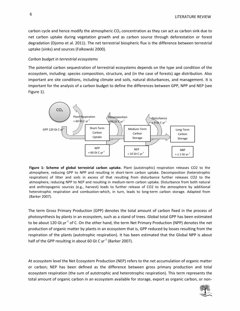
The potential carbon sequestration of terrestrial ecosystems depends on the type and condition of the
ecosystem, including: species composition, structure, and (in the case of forests) age distribution. Also
important are site conditions, including climate and soils, natural disturbances, and management. It is
important for the analysis of a carbon budget to define the differences between GPP, NPP and NEP (see
Figure 1).
The term Gross Primary Production (GPP) denotes the total amount of carbon fixed in the process of
photosynthesis by plants in an ecosystem, such as a stand of trees. Global total GPP has been estimated
to be about 120 Gt.yr-1 of C. On the other hand, the term Net Primary Production (NPP) denotes the net
production of organic matter by plants in an ecosystem that is, GPP reduced by losses resulting from the
respiration of the plants (autotrophic respiration). It has been estimated that the Global NPP is about
half of the GPP resulting in about 60 Gt C yr-1 (Barker 2007).
At ecosystem level the Net Ecosystem Production (NEP) refers to the net accumulation of organic matter
or carbon; NEP has been defined as the difference between gross primary production and total
ecosystem respiration (the sum of autotrophic and heterotrophic respiration). This term represents the
total amount of organic carbon in an ecosystem available for storage, export as organic carbon, or non-
CO2
Short-Term
Carbon
Uptake
Medium-Term
Carbon
Storage
Long-Term
Carbon
Storage
NPP
≈ 60 Gt C.yr-1
NEP
≈ 10 Gt C.yr-1
NBP
≈ ± 1 Gt yr-1
GPP 120 Gt C yr-1
Plant Respiration
≈ 60 Gt C yr-1
Decomposition
≈ 50 Gt C yr-1 Disturbance
≈ 9 Gt C yr-1
Figure 1: Scheme of global terrestrial carbon uptake. Plant (autotrophic) respiration releases CO2 to the atmosphere, reducing GPP to NPP and resulting in short-term carbon uptake. Decomposition (heterotrophic respiration) of litter and soils in excess of that resulting from disturbance further releases CO2 to the atmosphere, reducing NPP to NEP and resulting in medium-term carbon uptake. Disturbance from both natural and anthropogenic sources (e.g., harvest) leads to further release of CO2 to the atmosphere by additional heterotrophic respiration and combustion-which, in turn, leads to long-term carbon storage. Adapted from (Barker 2007).
LITERATURE REVIEW 7
biological oxidation to carbon dioxide through fire or ultraviolet oxidations. Heterotrophic respiration
includes losses by herbivores and the decomposition of organic debris by soil biota. It has been reported
that Global NEP is around 10 Gt.yr-1 of C. NEP can be measured in two ways: One is to measure changes
in carbon stocks in vegetation and soil; the other is to integrate the fluxes of CO2 into and out of the
vegetation (Barker 2007; Xiao et al. 1995; Lovett et al. 2006).
There is carbon uptake into both vegetation and soils in terrestrial ecosystems. Current carbon stocks
are much larger in soils than in vegetation, particularly in non-forested ecosystems in middle and high
latitudes (Barker 2007).
Carbon in forests
Forest exchanges carbon naturally with the atmosphere through photosynthesis, transferring the carbon
to their trunks, limbs, roots, and leaves as they grow. When leaves or branches fall and decompose, or
trees die, the stored C will be released by respiration and/or combustion back to the atmosphere or
transferred to the soil. Because of these processes, forests and forested landscapes can store
considerable carbon and their growth can provide a carbon sink (Falkowski 2000; Brennan et al. 2007).
Human activities change carbon stocks in these pools and fluxes between them and the atmosphere
through land use, land-use change, and forestry, among other activities
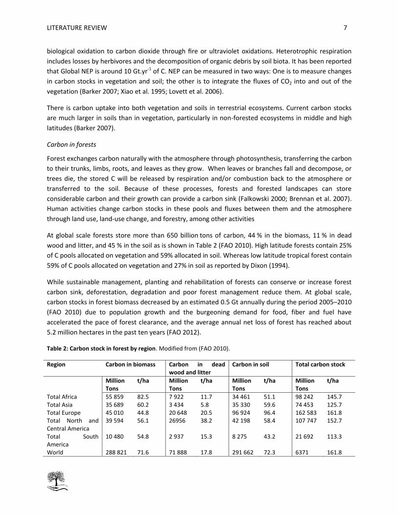
At global scale forests store more than 650 billion tons of carbon, 44 % in the biomass, 11 % in dead
wood and litter, and 45 % in the soil as is shown in Table 2 (FAO 2010). High latitude forests contain 25%
of C pools allocated on vegetation and 59% allocated in soil. Whereas low latitude tropical forest contain
59% of C pools allocated on vegetation and 27% in soil as reported by Dixon (1994).
While sustainable management, planting and rehabilitation of forests can conserve or increase forest
carbon sink, deforestation, degradation and poor forest management reduce them. At global scale,
carbon stocks in forest biomass decreased by an estimated 0.5 Gt annually during the period 2005–2010
(FAO 2010) due to population growth and the burgeoning demand for food, fiber and fuel have
accelerated the pace of forest clearance, and the average annual net loss of forest has reached about
5.2 million hectares in the past ten years (FAO 2012).
Table 2: Carbon stock in forest by region. Modified from (FAO 2010).
Region Carbon in biomass Carbon in dead wood and litter
Carbon in soil Total carbon stock
Million Tons
t/ha Million Tons
t/ha Million Tons
t/ha Million Tons
t/ha
Total Africa 55 859 82.5 7 922 11.7 34 461 51.1 98 242 145.7 Total Asia 35 689 60.2 3 434 5.8 35 330 59.6 74 453 125.7 Total Europe 45 010 44.8 20 648 20.5 96 924 96.4 162 583 161.8 Total North and Central America
The recently accelerated pressure on forest resources in order to provide environmental services,
including mitigation of atmospheric carbon dioxide, has increased the studies in forest cover and land
use. Allowing a better understanding on how these changes affect the emissions of CO2 to the
atmosphere, and how forests may be managed for carbon benefits (Hudak et al. 2012).
Direct determination of changes in terrestrial carbon storage has proven extremely difficult. Rather, the
contribution of terrestrial ecosystems to carbon storage is inferred from changes in the concentrations
of atmospheric gases, especially CO2 and O2, their isotopic composition, inventories of land use change,
and allometric models (Falkowski 2000; Dixon et al. 1994). Moreover, remote sensing approaches for
quantifying components of forest biomass are rapidly evolving; Hudak et al. (2012) suggested that to
quantify aboveground forest carbon pools and fluxes across broad extents, it is important to combine
remote sensing techniques with carbon estimation methods that are based on existing standard forest
inventory principles.
2.2.1 Environmental factors determining carbon storage in forests
For plant growth the distribution of fixed carbon is a primary determinant factor. Environmental
parameters, including resource availability and climate, greatly influence carbon allocation. Theoretically
plants adjust their allocation pattern to maximize growth (Tilman 1988). A plant in an environment
saturated of resources reaches its maximum growth rate by allocating all newly acquired
photosynthesized material to leaves, because the allocation to non-photosynthetic tissue yields no
returns in future carbon acquisition (Tilman 1988 & Friedlingstein 1999). The fraction allocated to leaves
influences canopy leaf area, leaf life time, photosynthetic capacity, flower and fruit production and
consumption, litterfall rates, decomposition and consumption by soil fauna. While, the fraction allocated
to fine roots and exudates influences water uptake, nutrient acquisition and the soil faunal communities
(Malhi et al. 2011).
Allocation plays an important role in the integration of plant responses to multiple stresses. Tilman
(1988) & Malhi et al. (2011) argues that competition for light and nutrients are the most important
factors determining biomass allocation. Responses to other factors, including water stress and elevated
CO2 could, however, also be important.
The optimal partitioning theory suggests that plants should allocate biomass according to the most
limiting resource (Malhi et al. 2011). Several studies showed that plants allocate relatively more carbon
to roots when water or nutrients are limiting and to shoots when light is limiting. Friedlingstein (1999)
considered three limiting resources: light, water and nutrients. Also climatic factors affect carbon
allocation, for example immediately after a severe El Niño there is a major shift in allocation (Paoli &
Curran 2007).
Shifts in CO2 concentrations also affect the allocation of carbon, under elevated CO2 levels more carbon
is partitioned to the aboveground compartment. The allocation component of the CO2 response is,
however, a secondary effect in comparison to the NPP response (Friedlingstein et al. 1999). Most
dynamic global vegetation model (DGVM) simulations suggest that rising concentrations of CO2 and
increasing temperatures will stimulate tree growth across most of the Earth’s surface, so increasing
LITERATURE REVIEW 9
globally averaged productivity and potential vegetation biomass stores through to at least the mid-21st
century (Keeling & Phillips 2007). Biogeographic differences besides cause changes in allometric
partitioning between major tropical forest regions (Malhi et al. 2011). Competition is considered
another factor affecting carbon allocation as mentioned by Dybzinski (2011), who stated the possibility
of competitive allocation of NPP in invading trees as they compete with established trees, in old-growth
stands where the stand is dual-limited by light and nutrients. This light limitation induces high leaf and
stem allocation in tropical regions (Friedlingstein et al. 1999). The last concept is especially important
because the estimated biomass depends on the allocation pattern.
2.2.2 Factors determining aboveground storage
The carbon trading market has established the urgent need to improve our understanding of the factors
explaining spatial variation in aboveground biomass (AGB) in tropical forests, especially given recent
increment in carbon emissions resulting from deforestation, degradation, fire, and drought in tropical
regions (Baraloto et al. 2011; Newell 2000; Brennan et al. 2007; Barker 2007).
Three groups of factors have been proposed to explain spatial variation of AGB in tropical forests at
regional level, namely climate, soil and stand variables. The relation of these environmental descriptors
with the spatial variation of ABG can be better understood by analyzing Figure 2.
Figure 2: Representation of the hierarchical nature of the relationships between aboveground biomass (AGB) and stand and environmental descriptors. Modified from Baraloto (2011).
The effect of each environmental descriptor can be observed in Table 3. Climate variables contributed
strongly to the explanatory variation in all three stand descriptors, especially basal area. Whereas, soil
texture (percent sand) showed contrasting relationships, with a strong positive relationship with the
explanatory variation in mean wood specific gravity (WSG) and a strong negative relationship with the
explanatory variation in stand mean diameter at breast height (DBH). Soil phosphorus showed negative
relationships with explanatory variation in all three stand descriptors, especially basal area and DBH
(Chave et al. 2004; Malhi et al. 2006; Slik et al. 2010; Quesada et al. 2009).
LITERATURE REVIEW
10
Table 3: Summary of factors observed to explain spatial variation in aboveground biomass in tropical forests (+, positive correlation; -, negative correlation; *, contrasting reports). Modified from (Baraloto et al. 2011).
Group Factor Effect
Climate Total Precipitation + Dry season length -
Soil Topography * Texture * Exchangeable bases * Labile P * Type *
Stand Basal area + Density of large trees + Mean Tree Height + Mean Tree DBH + Mean WSG +
Less accordance exists when examining relationships between AGB of tropical forests and the physical
and chemical factors of soils between the studies reported. While some studies reported positive effects
on AGB of soil fertility measures including total nitrogen (N), soil phosphorus (P), and exchangeable
bases (Paoli & Curran 2007; Baraloto et al. 2011) suggesting that AGB may be limited by soil nutrient
availability, other studies reported lower biomass on more fertile soils, with higher turnover rates of
biomass resulting in lower standing stocks (Quesada et al. 2009). The third group of variables which
explains spatial patterns in AGB comprises descriptors of forest structure and composition, referred as
stand variables. Strong positive correlations may be expected between AGB and variables used in
allometric equations, including diameter, height, and WSG in addition to metrics of stem density and
basal area (Chave et al. 2004; Baraloto et al. 2011; Henry et al. 2010). It has been established that the
absolute size and height of the light intercepting organs (leaves) determine the carbon capture, not their
size or height relative to the rest of the plant (Dybzinski et al. 2011).
2.3 Carbon storage in tropical forests
Tropical and subtropical forests have accounted for more than 40% of global GPP and net carbon uptake
over the past two decades. Tropical forests are among the most productive ecosystems on the Earth,
estimated to account for about one-third of global NPP (Malhi et al. 2011; Baraloto et al. 2011). As such,
NPP is an important determinant of the amount of the organic material available to higher trophic
levels. It can also indicate the magnitude and turnover of the carbon and nutrient cycles of that
ecosystem, and potential response times to disturbance. Old-growth tropical forests store carbon at an
estimated rate of 0.5 tC ha–1.yr–1 which leads to a carbon sink of -1.3 GtC.yr–1 across all tropical forests
during recent decades (Achard et al. 2010). As is shown in Table 4, tropical forest hold the highest
carbon storage compared to other biomes around the world. Results of field studies have shown that
seasonally moist tropical forests maintain high gross and net primary production (GPP and NPP)
throughout dry seasons that extend up to 5–6 months (Xiao et al. 2005; Fehse et al. 2002; Nogueira et
al. 2008; Usuga et al. 2010).
LITERATURE REVIEW 11
Table 4: Global carbon stocks in vegetation and soil carbon pools down to a depth of 1 m. Adapted from (Barker 2007)
A comparison between the different biomes of the world shows that the highest mean annual
increment of carbon biomass occurs in the tropics (Djomo et al. 2011). This increment includes
photosynthesis and autotrophic respiration represented by aboveground and belowground (fine and
coarse roots) biomass growth being the principal components of the carbon budget in tropical forests
(Djomo et al. 2011). Therefore, carbon sequestration in tropical and subtropical regions has been
receiving increased attention because these forests grow year round and have intense photosynthetic
activity and a wide diversity of species (Chen et al. 2012; Schimel et al. 2001; Cao & Woodward 1998).
Moreover, the response of tropical forest to the increased concentrations of CO2 has been analyzed by
experimental studies with growing trees in open-top chambers that indicates that an increase of 300
ppmv in atmospheric CO2 concentration stimulates photosynthesis by 60%, the growth of young trees by
73% and wood growth per unit leaf area by 27%. It seems probable that there will be a similar response
in natural forest ecosystems. Tropical forests are a prime candidate for such a C fertilization response
because of their intrinsic high productivity; the crucial question is to what extent the productivity might
be limited by the low nutrient availability, in particular by low nitrogen or low phosphorus (Malhi &
Grace 2000).
Unfortunately, forests can also act as a carbon source and substantial amounts of carbon have been
released from forest clearing at high and middle latitudes over the last several centuries, and in the
tropics during the latter part of the 20th century. For the period 1997 to 2006, global net carbon
emissions resulting from land use changes, mainly deforestation in the tropics and peat degradation,
have been estimated at 1.5 GtC. yr–1 (in the range of 1.1–1.9 GtC yr–1 ); 1.22 GtC. yr–1 from deforestation
and forest degradation and 0.3 GtC.yr–1 from peat degradation (Achard et al. 2010).
Influence of nutrients in tropical forests
Nutrient availability controls key processes in all ecosystems on earth. Nitrogen (N) and phosphorus (P),
either individually or in combination, limit primary productivity in most terrestrial ecosystems. In turn,
plant adaptations to these nutrients limitations strongly control ecosystem rates of nutrient cycling.
LITERATURE REVIEW
12
Most lowland tropical forests occur on highly weathered soils, where much of the original P rich parent
material has been lost, and most of the remaining P is unavailable forming part of iron and aluminum
oxides. Nitrogen, by contrast, accumulates over time through biological fixation, and is therefore
expected to be relatively more available than P in old soils. Thus, it is generally believed that NPP is
limited by P in lowland tropical forest (Hedin et al. 2013).
Many researchers have suggested and observed that proportional allocations to foliage and stem
increase and allocation to fine roots decreases with increasing N availability in both forests and other
types of vegetation. These trends have been explained using optimization theory: optimal plants balance
their belowground and aboveground limitations and thus maximize growth rates. However, specifically
in the case of tropical forest two fertilization experiments have been conducted in lowland tropical
forests to directly test nutrient limitation. One found evidence for N and P co-limitation, and one found
evidence of limitation by N, P, and K (Hedin et al. 2013). These results differ from the traditional view
that lowland tropical forests are P limited. In such a framework, the tradeoff is between belowground
and aboveground resource acquisition, where capturing more of one resource necessarily means
capturing less of the other (Dybzinski et al. 2011). The amount of foliage increases with nitrogen
availability under nitrogen-limited conditions: because foliage is stoichiometrically constrained by
nitrogen availability, greater nitrogen availability allows for more foliage, which leads to greater carbon
fixation (Dybzinski et al. 2011; Malhi et al. 2011). Since soil texture, water availability, and nitrogen
mineralization rates are frequently correlated (Reich et al. 1997), it may be easy to find many naturally
occurring nitrogen availability gradients that are also potentially correlated gradients in these other
parameters (Dybzinski et al. 2011).
2.4 Secondary forests and reforested areas
The role of tropical secondary forests as a carbon sink, either by natural or man-induced regeneration, is
receiving increasing attention in the debate on the global carbon cycle and reliable estimates of their
carbon stocks are pivotal for understanding the global carbon balance and initiatives to mitigate CO2
emissions through forest management and reforestation (van Breugel et al. 2011). Indeed, over 40% of
the C stored in terrestrial biomass is stored in tropical forests of which 40% are secondary and in some
stage of regeneration (Fehse et al. 2002). The potential for CO2 sequestration by regenerating forests
and reforestation is considerable. It has been estimated that roughly one third of the global potential of
carbon sequestration due to forests could be accounted for by secondary forest regeneration in the
tropics. Being a natural process, forest regeneration also has the benefit of being relatively cheap and of
conserving biodiversity, water and soil resources (Fehse et al. 2002). Even if reforestation affects soil C
stocks at the local scale at small magnitude, it could trigger a significant change in the global C budget if
large agricultural land is converted to forest, but it generates the tradeoff between conservation of
forest area or agricultural land (Dou et al. 2013).
2.4.1 Importance of small sized trees
Young secondary forests constitute an important component of tropical landscapes and constitute a
major global carbon sink. However, these forests are dominated by fewer species and the largest
proportion of stand basal area is constituted by smaller-sized trees (Usuga et al. 2010; van Breugel et al.
LITERATURE REVIEW 13
2011). Frequently these young trees and small stems are not considered for carbon estimation because
of the time required for adequate measurement and the lack of local robust models for carbon
estimation (Baraloto et al. 2011). Nevertheless of these limitations, Baraloto (2011) highlights the
importance of smaller stems to carbon stocks, stating that AGB of stems with DBH between 2.5 and 10
cm varied by a factor of more than five, accounting for < 1% in some French Guianan forests to more
than 25% of total AGB in a Peruvian white sand forest. This result contrasts with reports that small trees
(< 10cm DBH) account for only 3% of aboveground biomass in French Guiana. 80 percent of biomass
estimates in lowland tropical forests are based on measurements of trees > 10cm DBH (Keeling &
Phillips 2007). Baraloto (2011) shows that small trees should be also take into consideration in biomass
estimations, particularly in edaphically extreme habitats such as white-sand forests.
2.5 Effects of reforestation on the environment
Many studies have reported changes in tropical soil physical properties after deforestation, whereas
studies on reforestation are scarce (Mapa 1995). However the effect of reforestation on soil properties
has been evaluated by soil microbial biomass carbon (MBC), which can be effectively used as an index to
evaluate soil quality because it is sensitive and measurable, and it is related to global carbon cycle, soil
quality, soil C/N ratio and linkage of plants and soil. Liu (2012) demonstrated that MBC significantly
increased after reforestation, suggesting that reforestation significantly improved soil quality (Liu et al.
2012).
Mapa (1995) demonstrated that the reforested land has higher steady infiltration rate when comparing
with cultivated and grassland areas. This is caused by better soil structure and more macro pores
created by root activity and high organic matter content. The soil water retention at any given suction
was higher in the reforested soil. Furthermore, the bulk density was lowest in reforested soils, indicating
high porosities. This illustrates that reforested areas can accept and store more water than cultivated
and grassland areas. The increased infiltration and water retention consequently decreases surface run
off and conserve soil and water, restoring the hydrological balance (Mapa 1995). Nonetheless, once soils
are severely damaged, they take more than 20 years to recover, and any efforts should be taken to
avoid severe degradation of forested lands (Liu et al. 2012). Additionally, as mentioned before
reforestation alters soil organic matter content and hence affects the availability of nitrogen (N) for
plant growth, which potentially impacts the net primary productivity of terrestrial ecosystems. As direct
consequence of reforestation there is a significant increase in soil organic C and N concentrations
compared to uncultivated areas, increasing values with age (Dou et al. 2013).
Parrotta (1997) suggest that reforestation causes a catalytic effect. It is explained by changes in
microclimatic conditions, increased vegetation structural complexity, and development of litter and
humus layers that occur during the early years of plantation growth. These changes point to increased
seed inputs from neighboring native forests by seed dispersing wildlife attracted to the plantations,
suppression of grasses or other light demanding species that normally prevent tree seed germination or
seedling survival, and improved light, temperature and moisture conditions for seedling growth.
LITERATURE REVIEW
14
2.5.1 Factors determining success in reforested areas
Many reforestation projects have partially or completely failed because the trees planted have not
survived or have been rapidly destroyed by the same pressures (agricultural expansion, uncontrolled
livestock grazing, logging, and fuel wood collection) that have caused forest loss and degradation in the
first place (Le et al. 2012; Barker 2007). Reforestation can vary ranging from establishing timber
plantations of fast-growing exotic species through to attempting to recreate the original forest type and
structure using native species. The objectives of reforestation are dependent on the priorities and
objectives of stakeholders, the costs and benefits associated with available rehabilitation techniques,
and the economic, social, and environmental values that traditionally have been focused on wood
production, erosion prevention and water flow management (Parrotta et al. 1997). Recently, the
objectives are being focused to socio-economic benefits, ecosystems goods and services, recreation and
wildlife conservation (Le et al. 2012).
2.5.2 Success indicators
Reforestation is a process with two main stages. First the establishment phase, which is a three to five
year period from when seed or seedlings are planted to when young trees have gained the site, forming
a relatively closed canopy and suppressing weeds. During the establishment phase of reforestation, the
survival and growth of planted trees, and the degree of canopy closure are of particular importance. The
most common indicators used for measuring establishment success are the survival rate of planted trees
and the area successfully planted compared to a target area (Le et al. 2012; Parrotta et al. 1997). The
second phase is when established trees grow, reproduce, and are harvested or eventually die. Le (2012)
refers to this as the building phase of re-vegetation. During this phase, the focus of success is on tree
growth, stand density, stem form (in the case of timber trees) and the production of non-timber forest
products (such as fruit and resins). Measures of vegetation structure provide information on wildlife
habitat suitability, ecosystem productivity, erosion resistance and the successional pathway of the
forests. Measures of species diversity provide information on wildlife habitat suitability and ecosystem
resilience (Le et al. 2012; Sayer et al. 2004).
2.5.3 Technical and biophysical constraints of reforestation
The technical and biophysical constraints related with reforestation mentioned generally by researchers
are shown in Table 5. These include: site-species matching, site preparation, tree species selection,
seedling production, quality of seeds and seedlings, time of planting, technical capability of
implementers, post-establishment silviculture, and site quality (Le et al. 2012). Generally rehabilitation
efforts have focused on the production of a very limited number of species, or restoration plantings that
aim to recreate the diverse forest ecosystem believed to have once occupied the site (Parrotta et al.
1997).
LITERATURE REVIEW 15
Table 5: Biophysical and technical drivers of success related to reforestation. Modified from (Le et al. 2012).
Drivers Comments
Site-species matching Poor site species matching could lead a high mortality rate and poor performance of seedlings.
Tree species selection Selection of appropriate species to meet livelihood needs, provide environmental benefits is the key to the long-term sustainability of reforestation.
Site preparation Past failure of plantations has shown that land preparation is an important factor in the survival rate of planted trees and tree growth performance.
Quality of seeds and seedlings
Physiological quality and seedlings affects the success of establishment growth rate of trees.
Time of planting Planting seedlings at the right time is crucial, since this directly affects the survival of the seedlings in the field.
Technical capability of implementers
Despite facing many technical problems, government agencies felt technically competent while the other actors felt they had inadequate technical capability and needed support.
Post-establishment silviculture
The maintenance of newly planted seedlings in the field is a crucial project component that affects the survival of the seedlings and the sustainability of reforestation initiatives.
Site quality Site quality is the sum of climatic, geologic, and edaphic factors that influence tree growth at a specific location.
Site-species matching is determinant for survival and growth of planted trees. Poor site-species
matching is the main technical problem leading to poor short-term survival and growth of seedlings. The
species selected for reforestation can have a large influence on the benefits derived from the tree
products and as well on the ecological benefits of the forest (Sayer et al. 2004; Parrotta et al. 1997; Le et
al. 2012). Wherever possible, native species should be given preference over exotics, in part to help
minimize this risk. Seedlings should be of good quality and spacing chosen to favor early canopy closure
(Parrotta et al. 1997). Therefore, the success of any reforestation effort strongly depends on species that
can fulfil the demands of local people and cope with the site conditions and predominant competing
vegetation (Le et al. 2012). Mixed plantations could contribute to diversity, while also providing
production gains and reducing pest damage (Le et al. 2012; Parrotta et al. 1997). Fast growing pioneer
species should have preference, particularly those known to establish and grow well on degraded sites,
e.g., Acacia mangium on imperata grassland sites in the tropics. Nonetheless, there is a real risk that
some planted species (notably certain Acacia species and Leucaena leucocephala) could ‘escape’ from
cultivation and become established as weedy invader plants well beyond the rehabilitation target area
(Parrotta et al. 1997).
The availability of a nursery to produce seedlings, as well as having a good seedling preparation process,
is a key factor. The growing of seedlings in a nursery is the main way of raising planting stock in the
tropics. Tree nurseries can provide optimum care and attention to seedlings during their juvenile stage,
resulting in the production of healthy, vigorous seedlings (Le et al. 2012 & Ochsner et al. 2001). Constantly
reforestation specialists have searched for the characteristics that increase seedling survival and growth
after planting but only in recent decades they realized that height and diameter are not the only
seedling traits affecting field performance (Rose et al. 1990). Now reforestation specialists realize that
cultural practices in the nursery affect how well seedlings perform in the field. For example,
LITERATURE REVIEW
16
undercutting and wrenching can have the dramatic effect of increasing root system size, which has long
been linked to improved survival. Top clipping can improve field survival of excessively tall seedlings by
lowering the shoot/root ratio. Altering fertilizer and irrigation schedules to encourage bud set and
induce dormancy can greatly improve frost hardiness in the fall, winter storability, and stress resistance
during and following planting. Currently, many nursery personnel emphasize selecting standards based
on height and diameter, because these are easily judged in the packing shed and are broadly correlated
with other factors of seedling quality. Attention is often on maximizing the number of seedlings that can
be shipped because they exceed the culling standards rather than on maximizing the number of
seedlings that will survive and grow well. The knowledge of these traits should be used to improve the
cultural techniques that tailor seedlings in the nursery (Rose et al. 1990).
In general, the desired seedling quality is free of disease, has a straight sturdy stem, a fibrous root
system that is free from deformities, a balanced root and shoot ratio, is hardened to withstand any
adverse conditions of the planting site, with good carbohydrate reserve and nutrient content, and
should be inoculated with symbiotic micro-organisms when necessary. The planting time is determinant
directly affects the survival of the seedlings in the field. The optimal time to plant tree seedlings is at the
beginning or in the middle of the rainy season (Le et al. 2012; Parrotta et al. 1997; Sayer et al. 2004).
2.6 Status of Forest in Ecuador
Regardless of human impact the Ecuadorian Andes still represent one of the “hottest” biodiversity
hotspots worldwide (Makeschin et al. 2008). The vegetation of Ecuador follows the three major
landscape complexes, the drier “Costa” with semi-deciduous and deciduous forests and savannas, the
evergreen Amazon rain forest in the “Oriente” and the vegetation of the Andes. Due to the altitudinal
gradient and the varying climatic situations, the Andes alone comprise eight of the total 15 vegetation
types recorded for Ecuador. The per-humid montane broad-leaved forest and the upper montane or
Elfin forests (Ceja Andina) are well developed on the eastern escarpment of the Andes and in the
northern part of the western Cordillera, but attenuate towards the drier South (Makeschin et al. 2008).
The extent of forest in Ecuador in 2005 was 10.8 million ha, which represents 39% of the land area (FAO
2007). It is assumed that more than 90% of Ecuador’s surface had been covered by forests originally
(Makeschin et al. 2008). The area of primary forests remained unchanged in recent years. This is
certainly due to the fact that a lot of primary forests were protected. Ecuador’s forest protection
statistics present 21% of all forests as protected in 2002. So it can be concluded that the main
deforestation must take place in secondary forests. Granting a deforestation rate of −1.7% means a loss
of approximately 198 000 ha.yr-1 of secondary forests (FAO 2007).
The evergreen mountain rain forests of Ecuador suffers the highest annual rate (1.7%) of deforestation
in the whole of South America (Makeschin et al. 2008). Reforestation with native species is considered a
preferable option for sustainable development. Until the year 2000, 167 000 ha of plantations were
successfully established in Ecuador. Today, about 90% of all forest plantations in Ecuador consist of
introduced species (Beck et al. 2008), mainly Eucalyptus spp. and Pinus spp. (i.e. E. saligna, E. globulus,
P. patula, P. radiata); i.e. in the coastal region mainly Eucalyptus sp. and Tectona grandis, and in the
Sierra mainly Eucalyptus sp., Cupressus sp., and Pinus sp. This can be explained by the good availability
LITERATURE REVIEW 17
of planting material, existence of clear silvicultural management concepts, proven good productivity,
but also the lack of knowledge regarding the management of the native species (Günter et al. 2009).
Because of ecological problems with these introduced species, more emphasis is nowadays put on
plantations with native species (Cedrela sp. and Tabebuia chrysantha) (Makeschin et al. 2008; Günter et
al. 2009).
In Ecuador, remnants of the forests in the densely populated ‘‘inter-Andean valley’’ (2000–4000 m),
between the two Andean mountain chains, nowadays cover no more than 3% of the original area and of
all Andean forests in Ecuador only 25% are left. If we only consider economically marginal agricultural
lands in the Ecuadorian Andes, there is already an area of hundreds of thousands of hectares that could
be used for carbon sequestration through forest regeneration. Those marginal lands are usually found
near the timberline at high altitudes (Fehse et al. 2002). Investments from developed countries into
carbon sequestration in the Ecuadorian Andes are already being made. An example is a recent
reforestation program, financed by the Dutch FACE foundation, which uses high altitude marginal lands
(up to 3800 m) for large-scale forest plantations (Fehse et al. 2002). Complementary, the present
research is part of a reforestation project being executed by the Flemish internet company TELENET who
decided to invest in the tropics, in order to compensate for its own greenhouse gas emissions. Together
with Mindo Cloud forest Foundation (MCF, www.mcf.ec/ ) as local cooperating partner organization, the
project coverer 346 ha that already have been planted over two Northern provinces in Ecuador (Bauters
2013).
2.7 Assessing Carbon Aboveground storage in ecosystems
In recent years, the estimation of biomass components has become important for environmental
projects, since biomass can be related to carbon stocks and to carbon fluxes when biomass is
sequentially measured over time (Návar 2009). Forest managers and researchers require biomass
equations to predict the growth of young forest stands. Predicting tree biomass is important for
developing indicators of forest productivity, quantifying patterns of forest succession, estimating
potential carbon sequestering in forest stands and modeling forest growth at both tree and stand levels
(Robert & Ter-mikaelian 1998; Peri et al. 2006).
2.7.1 Allometric Models
Generally, regional and national biomass and C stock estimates for aboveground biomass as well as for
individual tree components are derived from plot level forest inventory data by applying allometric
biomass equations and biomass expansion factors (BEF’s) (Peichl & Arain 2007; Chave et al. 2005).
Estimates of carbon stocks are generally produced by a valuation of the total biomass of the population
using one of two approaches. The first is to estimate wood volume for each tree using a volume
equation which is in function of diameter and height. Then wood volume is converted to mass using a
timber density, and then wood mass is converted to total tree biomass using a biomass expansion
factor. The other approach is to apply a regression equation that directly converts external
measurements, such as stem diameter and sometimes height, to total tree biomass (Losi et al. 2003).
For developing these equations ground and destructive measurements of individual trees are required
to calibrate allometric equations (Fayolle et al. 2013).
The use of allometric equations or allometric regression models is a crucial step in estimating above and
belowground biomass (Singh et al. 2011; van Breugel et al. 2011). These models have as objectives: to
evaluate some tree characteristics of difficult measurement from easily collected data such as DBH, total
height, or tree age (in the case of plantations). Generally, equations are linear, exponential, allometric,
or hyperbolic, and correlations are often very good (Mouvondy et al. 2005; Singh et al. 2011).
Because 1 ha of tropical forest may shelter as many as 300 different tree species one cannot use
species-specific regression models, as in the temperate zone. Instead, mixed species tree biomass
regression models must be used (Chave et al. 2005). Furthermore, site-specific factors such as varying
tree density, soil moisture, nutrients, light, topography, and disturbance may affect tree allometry
(Peichl & Arain 2007; Usuga et al. 2010). At a local scale, the simplest models are based only upon tree
DBH. At regional or global scales, models based only upon diameter may have a greater associated
uncertainty than more complex models. Regarding this problem, tree biomass estimation can be
significantly improved by including wood density and tree height in the allometric models in addition to
tree diameter. However, measuring height and wood density requires additional work, increasing
project time and costs (Alvarez et al. 2012; Chave et al. 2005; Peichl & Arain 2007).
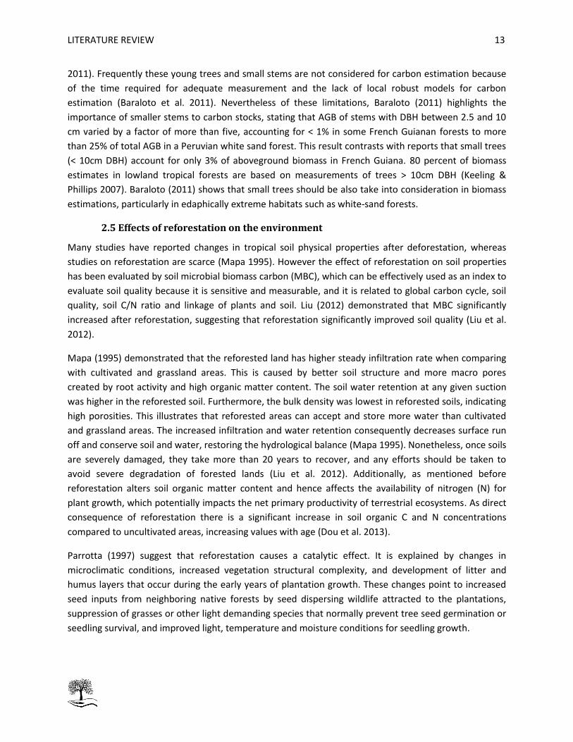
Figure 4 describe the process for converting forest plot data into regional-scale AGB estimates and how
during this process the error is propagated. Each tree inside a plot is measured, tagged and identified;
an allometric equation is used to relate its diameter to an AGB estimate. Then, the plot level estimate is
summed over all the trees to obtain a stand-level AGB estimate. For carbon sequestration issues, the
quality of this estimate depends on the plot size. In addition, the landscape-scale environmental
variability should be integrated by replicating the measurement in other plots of the same forest. These
steps integrate a variety of techniques that all contain some uncertainty, yet there is no consistent
methodology for propagating uncertainty across scales (Chave et al. 2004).
LITERATURE REVIEW 19
Figure 3: The error propagation for estimating the ABG of a tropical forest from permanent sampling plots. Modified from (Chave et al. 2004).
Other methods of biomass estimations include the combination of forest inventories with allometric
tree biomass regression models and airborne or satellite-based remote-sensing techniques (van Breugel
et al. 2011). In this sense, Geographical Information System (GIS) technology coupled with field
information offers a possibility to improve accuracy in estimating biomass and carbon densities and
pools in large areas. GIS allows incorporating different vegetation and other heterogeneity of the
landscape such as topography in estimates of carbon pools. It offers therefore a possibility to produce
biomass pool maps at local or regional level. Through this process, the result of ecological features can
be extended with more confidence to areas for which there is lack of data (Djomo et al. 2011).
2.7.2 Allometric Equations for small diameter and young trees
A correct evaluation of carbon storage within the ecosystem is of major importance, especially when
these storages are low (Mouvondy et al. 2005). Although abundant equations for biomass prediction
have been developed for mature trees, relatively few studies have focused on young trees (Robert &
Ter-mikaelian 1998). Results indicate that models that focus on large diameter classes, such as the
Chave and Brown models, consistently overestimate AGB for smaller diameter, indicating that the
development of allometric models for smaller size classes is particularly important in young secondary
forests (van Breugel et al. 2011). The errors in estimates biomass stocks are the result of absence of
allometric equations for smaller diameter class (below 10 cm) which have faster growing rate than the
higher diameter class trees (Singh et al. 2011). A few biomass equations for trees in seedling and sapling
stages have been developed for assessing the potential of young stands as fiber sources, as an indicator
of net primary production and for other purposes (Robert & Ter-mikaelian 1998). Some of them are
showed in Table 6.
LITERATURE REVIEW
20
Table 6: Allometric equations for young secondary forest. The models predict aboveground tree biomass (AGB) based on diameter at breast height (DBH) and wood specific gravity (WSG). N is the number of trees on which the models are based. DBH provides the DBH-ranges of the sampled trees. Modified from (van Breugel et al. 2011).
Author of the Model Model: AGB= Region N DBH(cm)
Kenzo et al. 2009 ( ( )) Malasya 136 0.11-28.7
Ketterings et al. 2001 ( ( ) ( )
Indonesia 29 7.6-48.1
Nelson et al. 1999 ( ( )) C. Amazonia 132 1.2-28.6
Sierra et al. 2007 (
( ))
Colombia 152 0.9-40
MATERIALS AND METHODS 21
3. MATERIALS AND METHODS
3.1 Study area
The monitored sites are distributed in two provinces of the north part of Ecuador; Pichincha and
Imbabura. At the moment the reforested zones correspond approximately to a surface area of ~ 350 ha,
distributed across different landlords, and can be classified in five different clusters according to altitude
(see Table 7 and Figure 4). In the future the reforestation project aims to expand to other parts of the
country.
Figure 4: Location of the study area, with an overview of each one of the five strata. The left picture indicates Ecuador and its borders (yellow line), the right picture depicts a zoom in the project area. The different strata are indicated as S1, S2, S3, S4 and S5; showing how stratum 5 and stratum 4 are a parallel transect to the one formed by stratum 1, 2 and 3. Strata 4 and 5 are situated in the dryer Imbabura province, and 1, 2 and 3 in wet Pichincha.
MATERIALS AND METHODS
22
Imbabura clusters
The clusters of Imbabura are located in the rural areas of the province in the inter-Andean valley where
the climatic conditions are more severe and dryer than those located in Pichincha. The project covers a
transitional zone running from Salinas at 1750 meters altitude to San Geronimo on the sub-tropical
western slopes of the Andes around 900 meters altitude and is made up of two strata.
Salinas (Stratum 4) is a small parish located 30 km away from the main city Ibarra. It is a valley
surrounded by two rivers Mira and Tahuando. This site is on a plain with no significant elevations. This
area is characterized by a very dry soil, without good physical structure or aggregates. The vegetation of
the zone is characterized by dry pre-montane forest, with an average rainfall between 500-1000 mm
(Bauters 2013 & Mindo Cloudforest Foundation 2011). San Geronimo (Stratum 5) is part of a small
village of La Carolina parish. Its vegetation is composed of dense pastures with scarce remnants of dry
pre-montane forest and wet tropical forest. It has a shallow mineral topsoil with an annual precipitation
estimated on 1500 mm (Mindo Cloudforest Foundation 2011).
Both of these sites originally used to be primary tropical montane forest (TMF) that were gradually
cleared after the construction of the railway from Ibarra to San Lorenzo (communication local people).
Nowadays there are only poor remnants of the forest. Figure 5 A and B, provide an impression of the
current situation.
Table 7: Overview of the different clusters and their location, with information on the altitude of each cluster and the reforested surface area. The names denoted are the same as used in the project description of Bos+ Tropen and Mindo Cloud Forest Foundation. Modified from Bauters (2013).
Name Altitude (m.a.s.l) Province Stratum Area (ha)
These clusters are formed by the Strata 1, 2 and 3 which are located in Cantons Quito, San Miguel de Los
Bancos and Pedro Vicente Maldonado respectively, which are part of Pichincha province. These
stratums (1-3) are made up of 30+ year old grasslands near to areas of eco-tourism. The three strata
follow an altitudinal transect between 2300 meters and 350 meters, ranging from montane cloud forest
to coastal foothills evergreen forest (Mindo Cloudforest Foundation 2011). These stratums are
characterized by very moist conditions with an average annual rainfall between 2000-4500 mm. On the
slope, there are still some patches remnants of tropical montane forest as is observed in Figure 5 C, D
and E. An overview of the climatic conditions in the five strata is given in Table 8.
MATERIALS AND METHODS 23
Table 8: Characteristics for the different strata. The Mean Annual Temperature (MAT) and annual Rainfall were provided by INAMHI. The average SOC and soil type were reported by Bauters (2013).
Average SOC (%) 1.92 2.18 4.40 0.33 1.93 Soil Type (WRB) Aluandic
Andosol Aluandic Andosol
Aluandic Andosol
Haplic Andosol
Vertic Andosol
Figure 5: Images depicting the panorama between the different stratums. A) Reforested area at stratum 4 (Salinas), B) Reforested area at stratum 5 (San Gerónimo), C) Reforested area at stratum 1 (Santa Rosa) with natural tropical montane forest at background, D) View from the highest part of stratum 1, patches of uncorrupted forest still remain to show the contrast with the other stratums, E) Stratum 3, crossed by two rivers.
A B
C
D
E
MATERIALS AND METHODS
24
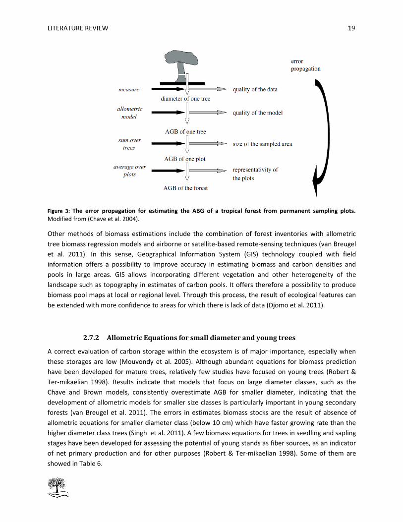
3.2 Tree inventory inside circular permanent sampling plots (PSP)
The inventory was performed on the PSP that were placed during the first field campaign (2012) of the
project. The detail of the number of plots placed and the number of plots inventoried is shown in Table
7. There is a difference between plots placed and found in stratum 1 because part of the reforested land
does not belong to the project anymore, meaning 4 plots have been removed. In total 40 PSP were
inventoried within circular plot of radius equal to 8m as performed by Bauters (2013) during soil carbon
estimation of the reforested areas.
Table 9: Detail of the number of PSP placed on 2012 per stratum and the PSP monitored on 2013.
Stratum Name Number of PSP placed
Number of PSP found and monitored
1 Santa Rosa 16 14 2 Piedras Negras 8 8
3 Suamox 4 4 4 Salinas 6 4
5 San Geronimo 10 10
3.2.1 Plot location
The location of the PSP for monitoring was done based on the information provided from the last year
campaign (2012), considering the following aspects: latitude and longitude of the established PSP and
altitude reported. Once the PSPs were located, the circular area around them was delimited using a rope
8m length as radius.
Figure 6: Graphical representation of the circular plots for monitoring. The radius of the plot equals 8m considered from the center of the plot which was marked at establishment in 2012 with bricks or cement signals.
3.2.2 Tree location
The documentation of tree location inside the PSP was necessary for future monitoring campaigns. In
order to report the location of each tree, the center of the plot was used as reference. A compass was
used to determine the angle of deviation between the geographical North and the tree and the distance
r=8m
MATERIALS AND METHODS 25
in meters from the center. Trees at the edge of the plots were included if more than 50 % of the trunk
were inside the plot (Phillips et al. 2009).
3.2.3 Tree diameter measurement
The diameter was measured in mm at 1.3 m height using a digital caliper when the tree was tall enough.
When deformities or buttress roots where present at this height, the point of measurement (POM) was
altered and recorded (Hoover 2008; Phillips et al. 2009). To define POM a pole with 1.3 m marked was
used to push firmly into the litter layer over the mineral soil next to the tree (Phillips et al. 2009). In the
case of trees smaller than 1.3 m, the diameter was measured at the collar (RCD) in mm at the soil
surface after removing coarse debris as recommended by Blujdea et al. (2012). For trees higher than 1.3
m both measurements were recorded (DBH and RCD).
Special considerations were made in case of forked trees, stump sprouts, trees with surface
irregularities, leaning trees, live wind thrown trees, and downed trees with tree-form branches growing
from the main bole (Blujdea et al. 2012, Phillips et al. 2009).
Deformities: for trees with irregularities at 1.3 m such as swellings, bumps, depressions, and
branches, measurements were made 2 cm immediately above the irregularity. The POM height
was recorded.
Fluted trees: for trees that were fluted along their entire stem measurement was considered to
be at 1.3 m.
Slopes and fallen or leaning trees: the DBH was measured from the downhill side of the tree as
is shown in Figure 7. Trees that were fallen or leaning always were measured at 1.3m length
along the side of the stem closest to the ground. In the case of fallen trees when it was
complicated to define the base of the trunk accurately, the measurement was 30 cm below the
tag.
Figure 7: Determination of DBH or POM in case of slopes (left) or fallen or leaning trees (right). Figure from Phillips et al. (2009).
Resprouts: in the case of standing but broken trees, or fallen individuals. The measurement was
done on the main stem or resprouts at 1.3 m from the base of the stem. A resprouting individual
was included only if the resprouts were greater than 1.3 m from the stem base.
MATERIALS AND METHODS
26
Multiple stems: all stems greater than 10 cm of diameter at 1.3 m of height were measured and
recorded.
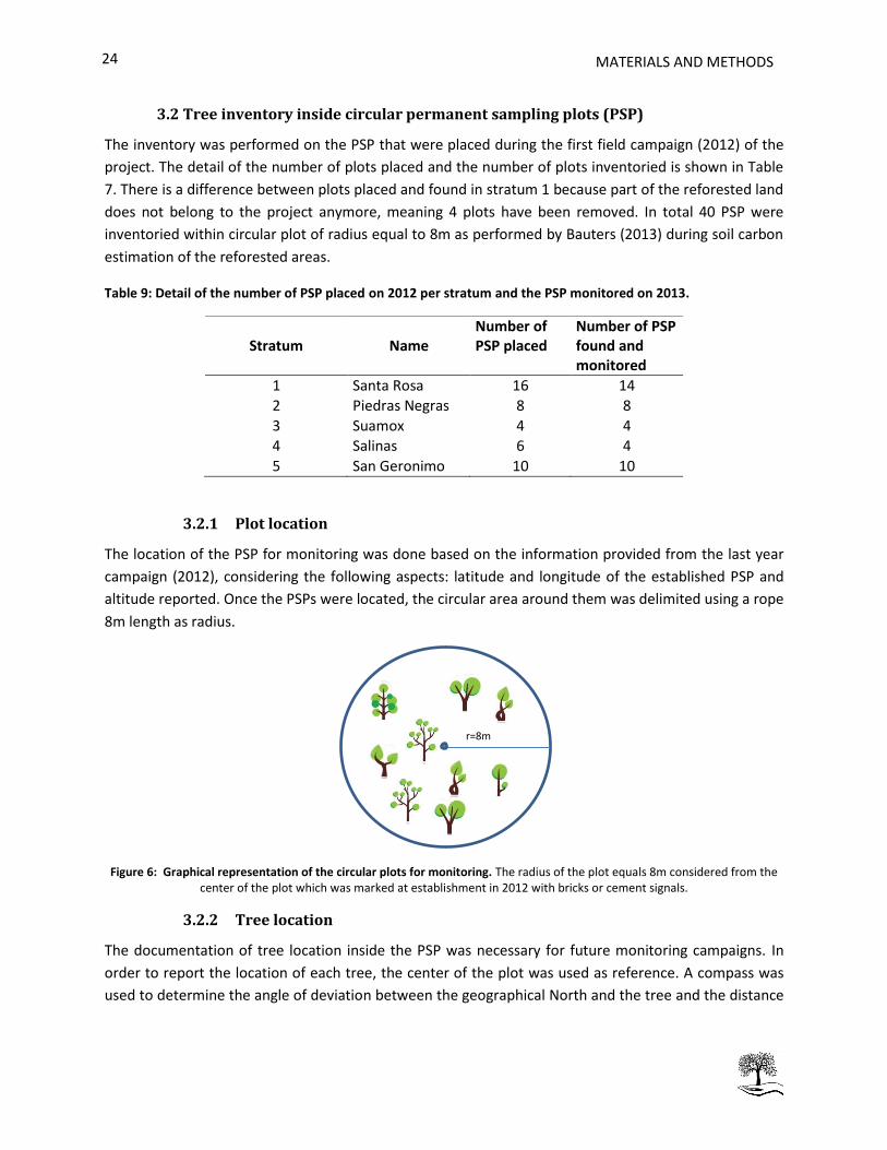
3.2.4 Tree height measurement
In the case of trees were higher than 1.8 m the measurement was performed according Chave (2006)
using an electronic hypsometer (Haglof Vertex III). This technique required to find a spot with a clear
view of the tree stem at around 10 m of distance. The precise horizontal distance from you to the stem
was measured using the electronic hypsomenter (Bauters 2013). Then laser was fired vertically
indicating the light to the crown. This procedure was repeated from several points directly below the
crown of the tree. The height was reported as the height of the observer plus the distance of the
furthest return for the laser (H1+H2) as is showed in Figure 8. In the case of trees smaller than 1.8m the
measurement was done using a metric tape.
Figure 8: Measurement of tree height using an electronic hypsometer. Figure from (Phillips et al. 2009).
3.2.5 Mortality and recruitment
In the cases where dead trees were found inside the circular area it was necessary to report the mode of
death: fallen, broken, standing (i.e. with branches intact). There are a special set of codes suggested by
Phillips et al. (2009) for refer about tree status (alive + dead). See Appendix section 7.1.
3.2.6 Tree identification
As these strata are reforested areas, the names (gender and species) of the planted trees are known, the
recognition was made with the help of local people who worked for the plantation and/or in the
nursery. Few trees could not be identified in field because they had not leafs for a visual identification or
in other cases because the plant was really small which made it difficult to recognize some
characteristics of the plant. In these cases a photographic inventory was made. These pictures were
analyzed by the responsible of the project who identified a few of them. The others were documented
as NI (not identified).
MATERIALS AND METHODS 27
3.3 Model selection
For selecting appropriate allometric models in this study, three criteria were considered. First, as in this
work the majority of the inventoried trees were smaller than 1.3m height; models that include tree
height as parameter were excluded considering the results of Peichl & Arain (2007), who stated that
biomass of all above- and belowground tree components are highly correlated to DBH, mentioning that
the addition of tree height or age did not improve the equation fit within any of the young stands tested
on their work, also mentioned by (Pajtík et al. 2008).
Secondly, previously published pan-tropical models as Chave's and Brown's were excluded considering
the nature of the study area (altitudinal gradient). This criterion was based on the conclusion of Alvarez
et al. (2012) about the useless of the Chave's forest type classification for differentiating variation in tree
form among forest types along the altitudinal gradient in Colombia causing variation in the resulting
AGB and introducing bias. Moreover, Preece et al. (2012) conclude that in relatively young forest stands,
such as the plantings investigated here, models that exclude stems <10 cm dbh are not appropriate for
carbon accounting as is the case of Brown’s model which was based on based only on stems ≥10 cm
dbh.
Finally, equations using wood density as a parameter were excluded considering that young trees have
higher wood density than older trees and that wood density slowly decreases, as the trees grow older
and eventually increases again in older stands as the annual rate of growth abates (Pajtík et al. 2008).
The resulting selected models are detailed in Table 10, these models are for AGB estimation in
secondary forest and were constructed including small diameter (DBH) ranges.
Table 10: Diameter-based allometric equations for aboveground biomass estimation. N is the number of trees on which the models are based. DBH provides the DBH-ranges of the sampled trees. AGB is the dry biomass of a tree in Kg. Modified from (van Breugel et al. 2011).
Nelson et al. 1999 xp( 1.97 2.41 ln(DBH)) C. Amazonia 132 1.2-28.6
Sierra et al. 2007 087 exp( 2.2 2 2.422 ln(DBH)) Colombia 152 0.9-40
3.4 Data processing
Due to the limitations of using the selected allometric models, other parameters as basal area (BA) and
tree height were analyzed for being considered a more real indicator of biomass. Then these results
were contrasted with the estimation of aboveground biomass using the selected allometric models.
Basal area (BA)
The basal area BA of the planting was estimated using the recorded RCD in cm. The estimation was
performed for each stratum as a complementary growth parameter. The estimation was performed
using R studio 3.03 free software.
MATERIALS AND METHODS
28
Mean tree height
The average height was estimated inside plots and then between plots to obtain a strata average height.
The calculations as well as the graph of height distribution among strata were performed on R studio
3.03 free software.
Aboveground Biomass (AGB) estimation
Diameter measurements were used to parameterize allometric relations for every plot. Firstly a relation
between DBH and RCD was established for trees which allowed recording both measurements with the
purpose of via this relation predict a DBH based on RCD for the rest (trees smaller than 1.3m). The
possibility of establishing a linear relation to predict DBH based on RCD as well as a ratio relation
(DBH:RCD) were analyzed. Afterwards, the predicted DBH or the measured DBH were used as
independent variable for predicting AGB from a variety of published relationships (Table 10). The AGB
estimation from tree to strata level based on plot inventories involved three steps as described by van
Breugel et al. (2011) (1) the estimation of individual tree biomass, (2) the summation of individual tree
AGB to estimate plot AGB, and (3) the calculation of an across-plot average to yield a strata-level
estimate. Because of a destructive sampling was not possible the best AGB estimation was considered as
an average between all the assessed models as the most representative result. The AGB estimation was
performed on R studio 3.03 and the graphs were performed on Microsoft Excel 2010.
Aboveground carbon (AGC) estimation
It was assumed that C concentration was 50% of the dry weight of AGB (Losi et al. 2003; Manrique et al.
2011; Preece et al. 2012) . The amount of AGC was reported as Kg.ha-1 for each stratum. The estimation
was performed using R studio 3.03 software.
RESULTS 29
4. RESULTS
The goal was to estimate AGB for all plots along the different studied strata in order to evaluate the
amount of aboveground carbon stored. Problems were encountered in allometric estimations when
trees were smaller than 1.3 m, introducing an error. Therefore, other relevant parameters as basal area
and tree height were analyzed in order to have a better idea of the real AGB. We first show the results
of number of trees at each stratum then we present the results of basal area and tree height measures.
Finally we move on to AGB estimations and species distribution per stratum.
4.1 Number of trees
In total 595 trees were inventoried in this study, the number of inventoried trees per plot and per
stratum is detailed in Table 11. There were plots where almost no planted trees were found inside the
PSP. It happened mainly in stratum 1 where in addition 4 plots were discounted because the land now is
being used for other purposes. The stratum with the highest number of trees per hectare is stratum 3
(Suamox).
Table 11: Summary of number of trees per plot and per stratum. NA= No information available, it means that trees were not found on those plots or that the number of plot was not present in that stratum. * The total number of trees includes alive and dead trees.
Stratum
Plot number 1 2 3 4 5
1 NA 15 25 21 22
2 NA 17 13 10 12
3 NA 18 22 22 9
4 NA 16 23 26 13
5 1 21
15
6 24 21
14
7 15 24
10
8 15 27
13
9 8
12
10 16
6
11 5
12 5
13 1
14 1
15 24
16 21
17 2
18 10
* Total inventoried 148 159 83 79 126
Total per hectare 525.68 988.31 1031.82 982.10 626.55
RESULTS
0
The detail of mortality per stratum is detailed on Table 12. It is observed that in stratum 4 there is
absence of mortality. The highest mortality corresponds to stratum 5 with a mortality of 15.87%. The
main types of death were standing dead trees and vanished trees.
Table 12: Report of mortality type. The physical mechanisms of death are standing, vanished (found location, tree looked for but not found) and one of multiple deaths (see Apendix section 7.1 for detail of the mechanisms of death).
Physical mechanism of death Stratum
1 2 3 4 5
Standing 1 7 0 0 14
Vanished 6 11 6 0 0
One of multiple deaths 0 0 0 0 6
* Total inventoried 7 18 6 0 20
Percentage (%) 4.7 11.3 7.2 0 15.8
4.2 Basal area (BA) estimation
The estimation of the average basal area per stratum is detailed in Table 13. The strata with higher basal
area (stratum 2 and 3) show high variability which is denoted by the elevated standard deviation
encountered compared to the other strata. The basal area of strata 1, 2 and 3 was based on the RCD
while the basal area of strata 4 and 5 was based on diameter at POM (between 3 and 10 cm of height).
Table 13: Average basal area per stratum. The estimations were performed considering a PSP surface area of 201.1m
2
The distribution of the basal areas at each stratum can be observed in Figure 9. There is observed
outliers far dispersed from the mean in all cases with exception of stratum 1. The more dispersed values
The abovementioned variability between tree heights at each stratum in relation to the mean can best
be observed in the Figure 10, where the distribution of tree height per stratum is demonstrated. The
mean in the graph is much lower than values reported on Table 14. This is due to the outlier values in
the boxplots. So stratum 3 has higher trees on average, but stratum 2 has more variability which affects
the result at stratum level.
RESULTS
2
Figure 10: Boxplot of the tree height data from the five different planted stratums
4.4 Aboveground Biomass (AGB) estimation
Since most allometric relationships for estimating AGB use DBH, we need to quantify the errors from
using RDC measurements. 595 trees were inventoried in total, and from 39 of these trees both DBH and
RCD measurements were available. This data allowed determining the effect of using RCD instead of
DBH in the selected allometric relations for AGB estimations. This influence can be visually observed in
Figure 11, where regression lines for each tested model show the same regression equations but
different AGB estimations when using RCD instead of DBH as originally described in literature causing an
AGB overestimation in all cases when RCD was used as a predictor. It is possible to observe that Nelson
model show higher AGB estimations followed by Sierra model and Kenzo model which shows the lowest
estimations.
RESULTS 33
Figure 11: Influence of using RCD in allometric equations designed for DBH. The blue lines correspond to the regression lines of the tested allometric models when using RCD and the red lines when using DBH. For the legends, K: Kenzo model, N: Nelson model and S: Sierra model. The original allometric equations are described on Table 10. In this graph the values of x axis (DBH) correspond to the observed values from field measurements, while the aboveground biomass values (y axis) are an estimate based on the before mentioned allometric models.
The tested relations between RCD and DBH are showed in Figure 12. The first one shows a linear
relation using RCD as an independent variable to estimate DBH. The second one shows the DBH
estimation based on the DBH/RCD average ratio obtained from the 39 mentioned trees. The ratio used
was DBH=0.46 ± 0.14 RCD.
y = 0.083x2.43 R² = 1
y = 0.083x2.43 R² = 1
y = 0.1395x2.413 R² = 1
y = 0.1395x2.413 R² = 1
y = 0.1166x2.422 R² = 1
y = 0.1166x2.422 R² = 1
0
2
4
6
8
10
12
14
16
18
20
0 1 2 3 4 5 6 7 8
Ab
ogr
ou
nd
Bio
mas
s [k
g]
Diameter DBH or RCD [cm]
Aboveground Biomass vs RCD & DBH
K
K with RCD
N
N with RCD
S
S with RCD
RESULTS
4
Figure 12: Relations for predicting DBH based on RCD. In the upper graph, the linear regression for obtaining a DBH corrective equation based on RCD. Down the predicted values using a DBH/RCD ratio compared with the measured values, the vertical bars show the standard deviation from the measured values. The standard deviation was estimated between the measured values and the corrected ones.
From the 39 trees that had both measurements (DBH and RCD), 32 belonged to the Alnus sp. and only 7
were from different species. The correlation factor among the measured DBH values and the predicted
with the established ratio relation was 0.86 when using the 39 trees and 0.92 when using only the Alnus
trees.
The linear relation based on the regression between RCD (predictor variable) and DBH (dependent
variable) illustrated on Figure 12 upper part was discarded as an option. It demonstrated to be useless
for correcting DBH as it generate negative values for RCD smaller than 13.44 mm. For the following
estimations the corrected DBH based on the DBH/RCD relation was used when DBH was not available.
The distribution of the corrected diameters at each stratum is shown in Figure 13. The higher values
correspond to stratum 3 and 2, however it is observed from the graph that stratum 2 has more
variability. Similar situation is observed for stratum 1 and 5 which show high dispersion of the outliers.
y = 0.7096x - 9.5345 R² = 0.8472
-20
-10
0
10
20
30
40
50
0 10 20 30 40 50 60 70 80
DB
H (
mm
)
RCD (mm)
05
101520253035404550
0 10 20 30 40 50 60 70 80
DB
H [
mm
]
RCD [mm]
Measured values
Estimated DBH using DBH:RCDratio
RESULTS 35
Figure 13: Distribution of the corrected DBH per strata for the complete data set. The DBH estimations were performed using the relation DBH=0.46 RCD ± 0.14.
The estimations of dry biomass performed by using each selected model are shown in Table 15. The
standard deviation is higher in all cases for stratum 2 and 3 corresponding with the strata having higher
trees (Table 14).
Table 15: Aboveground biomass estimations using different allometric models for strata 1 to 5. The detail of each equation is on Table 10.
Stratum Aboveground biomass [Dry weight kg. ha-1]
Model Kenzo ± SD Model Nelson ± SD Model Sierra ± SD
Due to the uncertainty regarding accuracy of the tested models, the result of aboveground carbon is
reported as the average between individual AGB estimations of the tested models: Kenzo, Nelson and
Sierra (Table 16). The carbon content was considered 50% of the dry biomass. The standard deviation
shows the variation of the data per stratum, it is higher for stratum 2 and 3 than for the other strata.
The detail of the AGC estimation per individual plot is showed in Appendix 1.
RESULTS
6
Table 16: Average estimation of aboveground carbon. The estimation was performed using an average between estimations coming from three selected allometric models mentioned on Table 10. The altitude of each stratum is detailed.
The distribution of aboveground carbon in the monitored trees is depicted in Figure 14. The graph show
the average values obtained from the three tested models (models of Kenso, Nelson and Sierra).The
individual contribution of the monitored trees is depicted for each stratum. It is observed from the
graph that there is high variability for stratum 2 which show dispersed outliers.
Figure 14: Distribution of the aboveground carbon average estimation.
The relation between aboveground carbon storage across the different PSP of the different strata and
the altitude is demonstrated in Figure 15. While Figure 16 showed the average AGC (kg.ha-1) per
stratum. It is observed that there is not a clear relation between altitude and AGC, it is clearly confirmed
by stratum 2 which in average exhibit higher AGC stock than the lower strata 3 and 5.
RESULTS 37
Figure 15: Graph showing the AGC content in the inventoried permanent sampling plots on the different reforested strata spread over northern Ecuador. The strata are labeled with different colors. Blue S1 stands for stratum 1, red S2: stratum 2, light green S3: stratum 3, dark green S4: stratum 4 and purple S5: stratum5. The values considered the result from the average estimations between the three selected models (see Appendix 1).
Figure 16: Graph showing the average AGC content (kg.ha-1
) for the different reforested strata spread over northern Ecuador. S1: stratum 1, S2: stratum 2, S3: stratum 3, S4: stratum 4 and S5: stratum 5.
0
1
2
3
4
5
6
7
8
9
0 500 1000 1500 2000 2500
Ab
ove
gro
un
d C
arb
on
[kg
]
Altitude [m.a.s.l]
S1
S2
S3
S4
S5
0
20
40
60
80
100
120
140
160
0 500 1000 1500 2000 2500
Ab
ove
gro
un
d C
[kg
.ha
-1]
Altitude [m.a.s.l]
S1
S2
S3
S4
S5
RESULTS
8
4.5 Relation between basal area, tree height and AGC
The relation of AGC with basal area and tree height is represented in the upper and middle part of
Figure 17, it observed that the strata with the highest AGC stocks have the highest basal area as well as
the highest tree height (stratum 2 and 3). On the other hand the relation between basal area and tree
height at each stratum don not show a clear link. Nevertheless, for plots with a higher BA (stratum 2 and
3), a higher mean tree height is found and high variability.
Figure 17: Relation between aboveground carbon, basal area and tree height. The legends stands for, AGC: stands for aboveground carbon estimations, BA: basal area. The vertical bars represent the error for the standard deviation.
0
2
4
6
8
10
12
0
20
40
60
80
100
120
140
160
0 1 2 3 4 5 6
Bas
al A
rea
[m2
]
Ab
ove
gro
un
d C
[kg
.ha-
1]
Strata
AGC
Basalarea
-0.5
0
0.5
1
1.5
2
2.5
0
20
40
60
80
100
120
140
160
0 1 2 3 4 5
Tre
e h
eig
ht
[m]
Ab
ove
gro
un
d C
[kg
.ha
-1]
Strata
AGC
Height
-0.5
0
0.5
1
1.5
2
2.5
-2
0
2
4
6
8
10
12
0 1 2 3 4 5
Tre
e h
eig
ht
[m]
Bas
al A
rea
[m2
.ha
-1]
Strata
Basalarea
Height
RESULTS 39
The upper part of Figure 17 show discrepancy of basal area in relation with aboveground carbon as is
observed for strata 2 and 3, where stratum 2 showed the highest aboveground carbon storage however
the basal area per hectare is not the highest for this strata, being strata 3 the which one that shown on
average the higher basal area per hectare. Similar situation occurred with strata 4 where in spite of the
lower aboveground carbon storage the basal area is higher than for strata 5.
When ignoring the distribution of data per strata and the whole data set is considered it is possible to
identify a direct relation between basal area and AGC as depicted in Figure 18, as basal area increase
AGC estimation increases. However this relation is not linear, the increment of AGC follows a polynomial
pattern.
Figure 18: Relationship between aboveground biomass and basal area. Graph was developed with the information of the 572 from of the 595 analyzed trees. The polynomial regression showed to fit best with the data.
4.6 Species distribution and aboveground carbon storage
The variety of planted trees per stratum and the amount of aboveground carbon stored per species is
detailed in the Figure 19. It is possible to state that the species which accounts for more aboveground
carbon storage in strata 1 and 2 is the same (ID 2 which corresponds to Alnus sp.) while the other
species had a minor contribution. The details about the names of the species are showed in appendix 1
(see Table 17). In other hand in stratum 3 the main contributors for carbon storage are Inga sp. (ID 25)
and Inga spectabilis (ID 27). However, there are other minor contributors which account smaller
amounts of carbon, namely Gliricidia sepium (ID 23), Erythrina sp (ID 20), Cordia alliadora (ID 16),
Brownea hertae (ID 5) between others. In the case of stratum 4, the variety of planted trees is the
lowest being Casuarina equisetifolia (ID 10) the most representative species for aboveground carbon
storage. In the case of stratum 5 the main contributors are Psondias sp (ID 55), Gliricidia sepium (ID 23)
and Acacia macracantha (ID 1).
y = 0.0005x2 + 0.0238x - 0.0022 R² = 0.962
-0.5
0
0.5
1
1.5
2
2.5
3
3.5
0 10 20 30 40 50 60 70
Ab
ove
gro
un
d c
arb
on
[k
g]
Basal Area [cm2]
RESULTS
40
Figure 19: Tree species and its aboveground carbon stock distribution per strata. The species in the graph are designated with a number which is detailed in the appendix 1 (Table 18) with the full names of the corresponding specie. The aboveground carbon values correspond to the amount of carbon in each monitored tree.
DISCUSSION 41
5. DISCUSSION
This study seeks to establish the baseline estimation of carbon aboveground storage in the reforested
areas in northern Ecuador as part of the project founded by BOS+ and TELENET and executed by MCF.
These results are the first estimation of aboveground biomass since the plantation in 2012. The
retrieved results are very important because they provide with a general overview of the success of the
plantations. In addition, this data will be used as the baseline data for future monitoring. Furthermore,
the results contribute to the research of biomass estimation in seedlings in the tropics. A limitation of
this study is that the data analysis reflects only one point in time (first estimation). The results are
further discussed in the following sections.
5.1 Number of planted trees and specie on AGC
The results of density of planted trees are important because these directly affect biomass estimations.
The variable number of trees found (see Table 11) at each strata could be attributed to various factors
such as climatic (soil properties, weather), anthropogenic pressures (agriculture, cattle), site conditions
(vegetation coverage, fauna) and type of planted species. The results of stratum 3 and stratum 2,
showing higher number of planted trees per hectare, are attributed to the favorable climatic conditions
of the area (see Table 7 and 8). In the case of stratum 4, in spite of the low rainfall registered, a high
number of planted trees were observed. The latter can be attributed to the good soil properties (see
Table 8) and a dedicated care of the seedlings. This is supported by field monitoring observations where
a permanent worker in this stratum saw seen to be responsible exclusively for irrigating the seedlings,
weeding, and replanting in the case of dead trees. A similar situation was observed for stratum 3 where
two permanent workers were seen. At stratum 5 the reported mortality rate of 15% (see Table 12) could
be attributed to the non-favorable climatic conditions (Table 8) summed to the fact that the planted
area was completely covered by pasture which can be competing by nutrients and water with the
planted trees.
Our results also indicate that the type of planted species could influence the number of successfully
growing trees at each stratum. For example, the fast growth character of some tree species can be
attributed to their early successional (pioneer) status (Günter et al. 2009) as we reported in this study
for Alnus sp. The explosive growth of Alnus sp. in relation with the other species was also reported by
Fehse et al. (2002) during the first years of establishment in Alnus and Polylepis forests in Ecuador.
Moreover, it is known that mid- and late-successional species have a completely different physiological
behavior compared to early successional species and thus should respond to different vegetation stages
of planting sites (Günter et al. 2009). Other identified fast growing specie was Inga sp. which has been
reported to have a rapid germination and growth, tolerance of poor soils, nitrogen fixation and
mycorrhizal activity, as well as a great ability to coppice and weed control (Valle 2010).
We additionally found that the state of vegetative coverage at each stratum could be influencing species
succession and consequently AGC storage. Conventionally in reforestation activities, trees are usually
planted directly in areas that were manually or chemically cleared or burned. These conditions may be
more favorable for pioneer and many exotic species but not for mid-and late- successional species which
DISCUSSION
42
need shadow (Günter et al. 2009). This is confirmed in this study, at least in stratum 1 and 2, where
Alnus sp. (fast grower) showed to be possibly favored by the previous use of glyphosate. However, it is
still unclear if the glyphosate application had other kind of effects on the other planted species. This
could suggests that the rest of planted species, possibly mid- and late- successional species, would
possibly develop better in the future when shadow created by the pioneer species increases/rises. For
Alnus, it is expected that in its mature state the Alnus trees would have been replaced by other species,
a process that have been observed in 30- and 45-year-forests (Fehse et al. 2002).
Because each species has specific characteristics and growth requirements it would be important to
analyze carefully if the application of glyphosate is convenient or not in all strata. In spite of the lack of a
well-established reforestation procedure in the tropics to adapt tree species to the successional stage of
the dominating vegetation, there are some studies (Günter et al. 2009; Fehse et al. 2002; Girardin et al.
2010) that have already proven that in the tropics, a combination of early and late successional species
can provide better ecological and economic benefits. This would allow to expect a good development of
these reforested sites in the future, because as was observed during the inventory stage the plantations
have been designed as mixed plantations.
5.2 Relation of AGB with basal area and tree height
Basal area and tree height data were evaluated to be used as an AGB indicator. The latter was necessary
because no destructive AGB estimations were performed in this study, so it was not possible to verify if
the estimations obtained using allometric models from the literature described properly the situation of
the study area. Figure 15 shows that there is a relation between basal area and aboveground biomass.
This is supported by studies that demonstrated strong relationships between AGB and both basal area
and large stem density throughout several Neotropical forests (Baraloto et al. 2011; Chave et al. 2004;
Chiba 1998). This simple relationship has shown to be applicable to the aboveground biomass
estimation using BA in forest stands (Chiba 1998; Chave et al. 2004). The relationship between
aboveground biomass and basal area in a forest stand is likely to be associated with tree architectural
development because the lower part of the tree trunk contains the growth process of the tree since
initiation and obviously because DBH is used as the main predictor for AGB estimations (Baraloto et al.
2011). As shown in Table 13, Table 14, Figure 9 and Figure 10 both basal area and tree height pointed
strata 3 as the stratum with the highest potential for AGB storage followed by stratum 2. The high
performance of these strata agreed with the fact that both have fast growing species such as Alnus sp.
and Inga sp. with 28% and 25% of the planted trees at each stratum.
5.3 Importance of model selection and its influence on AGB estimation
As in this study it was not possible to perform destructive biomass measurements for developing site
specific equations or to choose the best fit relation from literature, the selection of the proper
allometric models from similar previous studies was of crucial importance. Depending on the selected
models the estimation approaches better to the real situation or introduces a bias. In this case the study
area corresponds to recent reforested sites where trees were mostly under 1.3 m height. This
introduced the question of which and how many predictor variables should be included in the models to
predict aboveground biomass for these young planted trees. Few allometric relations for young trees
DISCUSSION 43
were found (e.g Blujdea et al. 2012; Pajtík et al. 2008). Unfortunately these developed equations could
not be applied in this study due to their species specific character/nature. No non-specific allometric
models were found for young mixed plantations in the tropics. Consequently, we opted to select
multispecies equations developed for AGB estimation in secondary tropical forest which included small
diameter sizes. The diameter ranges included in these studies were from 0.11 to 28.7 cm, 1.2 to 28.6 cm
and 0.9 to 40 cm at DBH from Sierra et al. (2007), Nelson et al. (1999) and Kenzo et al. (2009)
respectively.
An additional obstacle was the use of DBH as the single predictor variable in the selected allometric
equations (see Table 10). In this study only 39 of the 595 inventoried trees were high enough to obtain
DBH; for the remaining trees RCD was recorded. For this reason we related RCD with DBH in order to
correct for the error introduced by the use of RCD for biomass estimation for those trees which height
was less than 1.3 m. By doing this transformation, the first source error in the biomass estimation was
introduced, because this RCD to DBH projection imply a biomass overestimation. In some literature (van
Breugel et al. 2011; Malhi et al. 2006; Chave et al. 2005), DBH is considered the most important
parameter for biomass estimations, but in the case of young trees or seedlings Pajtík et al. (2008), Kenzo
et al. (2009) and Blujdea et al. (2012) stated that stem base diameter (RCD) resulted to be the best
predictor for each compartment. In this study it was not possible to use the recorded RCD because the
available allometric equations required DBH as predictor (Table 10), increasing the error in the
estimation. It was demonstrated that using RCD in the same allometric model instead of DBH (Figure 11)
caused higher AGB estimations for the same tree. For this reason it was necessary to use the corrected
values of RCD.
In addition, we were not able to introduce other ecologically important variables such as wood specific
gravity (WSG) or tree height that have shown to improve AGB estimations (van Breugel et al. 2011;
Henry et al. 2010; Chave et al. 2005; Chave et al. 2004) because the selected equations did not consider
these parameters. Nevertheless, in the case of small trees and seedlings it has been suggested that
these parameters are not critical for the improvement of the estimations. Pajtík et al. (2008) in a study
on young Norway spruce and Blujdea et al. (2012) in a study on young planted trees in Romania
mentioned that using tree height (H) as a second independent variable did not significantly improved
the overall predictive power of the models. They argued that the influence of height was not detectable
and that this was probably caused by a high co-linearity coefficient between stem diameter and tree
height.
Finally, we wonder what would be the result of using pan-tropical models for broadly defined forest
types based on large, compiled data sets. We believe it may involve more of the community-level
allometric variability of a given forest than a local model (Chave et al. 2004; Fayolle et al. 2013; Djomo et
al. 2011; Losi et al. 2003). However, previous studies (van Breugel et al. 2011; Kenzo et al. 2009;
Ketterings et al. 2001; Sierra et al. 2007; Alvarez et al. 2012) indicate that models that focus on large
diameter classes, such as the Chave and Brown models, consistently overestimate AGB for smaller
diameter classes until 52% ± 10% (Girardin et al. 2010). These results emphasize that the forest
categories used by Chave et al. (2005) would not be ideal for carbon estimations in highly
environmentally heterogeneous countries, such as the Andean regions (Alvarez et al. 2012; Girardin et
DISCUSSION
44
al. 2010). For instance, the generalized pan tropical equations provided by Brown and lately by Chave
are valid for trees up to a DBH of at least 10 and 5 cm respectively (Henry et al. 2010). The last fact was
the main reason for excluding these models from our options since in this study the predicted DBH
This equation for total aboveground biomass was developed from a set of 52 secondary forest plots to
predict aboveground biomass. Considering this equation with 2 as stand age, the obtained value is 0.64
Mg.ha-1. The latter value is higher than the obtained from the 2 year reforested stratum 2. However, it is
necessary to consider that this equation was performed for established secondary forests.
Blujdea et al. (2012) reported aboveground biomass of seedlings about 2 years old (RCD = 10 mm), to
vary between 0.02 kg and 0.04 kg/plant. When converting the biomass estimation of our study up to
plant level we obtained for stratum 2 with 298.51 kg.ha-1 (Table 16) and 988.31 trees per hectare (Table
11) the resulting amount of aboveground biomass per tree of 0.3 kg/tree which is considerably higher
than reported by Blujdea. This difference could suggest that our results have been overestimated. Other
study in young pine plantations (2 years) reported aboveground biomass of 0.1 kg/tree (Peichl & Arain
2007). Because of the abovementioned reports correspond to different tree species the comparison is
not valid. However, a previous study in Ecuador reported aboveground biomass of 113.8 Mg.ha-1 for a 8
years Alnus forest and 77.3 Mg.ha-1 for a 6 years Polylepis forests (Fehse et al. 2002). The latter results
demonstrate that reforestation with native species could lead to high amounts of aboveground biomass;
turning in positive the future expectations of this reforested sites.
6.1 Analyzing error sources in the allometric estimations
The high variability regarding DBH and total height among planted trees made it difficult to use directly
allometric equations. Unfortunately, the transformed values RCD to DBH introduced a bias. This, in
addition to the lack of proper allometric models for mixed tropical seedlings, caused that our results
become just a general idea of the situation but not an accurate estimation.
The different times of plantation as well as the replanting practice during the establishment phase was
the main reason to find trees at different growth stages. These differences generated large standard
deviations among the data, especially for stratum 2 and 3 (Table 11 and Table 2). The elevated standard
deviations showed to us that there is no homogeneity among population, as observed in Figure 9, Figure
10 and Figure 13 where for stratum 2 and 3 some of the data is far dispersed from the mean population.
This dispersion (extreme values) is the reason of higher biomass estimation for stratum 2, however,
does not represent the situation of the majority of population. Ignoring the differentiation of wood
density between species can also affect the AGC estimation as pioneer species hold generally lower
WSG than slow growing species. Other sources of error are reported to be linked on how well the census
was performed, and how large the census was (Chave et al. 2004). In this line it can be mentioned that
the number of PSP placed was properly calculated by BOS+ Tropen employing the Winrock Terrestrial
Calculator and the surface area of the PSP was suggested by Bauters (2013) according to Phillips et al.
DISCUSSION 49
(2009). Other methodological sources of error that could happen in this study include the incorrect
estimation of the plot area, trees missed or measured twice (Chave et al. 2004; Djomo et al. 2011).
CONCLUSSIONS
50
7. CONCLUSSIONS
Research on carbon aboveground estimations in seedlings and reforested areas in the tropics is still in an
early stage. Therefore, this study is a valuable contribution to increase knowledge on this topic. This
study is possibly the first of its type in Ecuador and is of crucial importance for establishing a base line
for future monitoring campaigns on the reforested areas of the project, but as it is the first estimation
(only one point in time) the scope of the analysis remains limited.
The above ground biomass estimations based on allometric equations for secondary forest introduced
error in the estimations performed. Firstly because these equations were performed for consolidated
forest, and secondly because the equations used diameter a breast height as single predictor variable
and this parameter was not available in all of the cases as the majority of trees were smaller than 1.3 m.
Also, the correction used for DBH in the allometric models introduced another source of the error in the
estimation. As an alternative, basal area and tree height performed well as biomass indicators.
The analysis based on basal area and tree height as indicators of aboveground biomass suggested
stratum 3 to have on average the largest carbon stock of the reforested sites. However the presence of
some trees, which demonstrated extreme values regarding corrected DBH at stratum 2, caused a shift in
the results when comparing with the allometric estimations. The allometric models, indicated stratum 2
to be the major pool of aboveground carbon. The results suggest that the presence of extreme values
(bigger trees with bigger DBHs) increase the estimated value of carbon from population to stratum level.
The allometric relations between aboveground biomass and diameter at breast height follow the
pattern of a power function and higher increments for big diameter trees are observed.
With exception of stratum 2, a relation was reported between aboveground biomass and altitude,
meaning that biomass decreased as altitude increased. The high performance documented on stratum 2
is probably occurring due to the presence of the fast growing specie Alnus sp. which accounted for
79.7% of aboveground biomass summed with the favorable climatic conditions of the area. In the case
of stratum 3 the results are attributed to the presence of Inga sp., other fast-growing specie which
accounted for 40% of the biomass. The lower carbon stocks were founded in stratum 1 and stratum 4.
In the former low carbon stocks were caused cause of the low number of planted trees per hectare and
the influence of the altitude. The latter was due to the extreme climatic conditions as this stratum
possess the minimal annual precipitations and due to the effect of the altitude. In all cases, the type of
planted species influenced the performance of each stratum as it were identified fast growing species
such as the abovementioned and mid- and late-successional species as with Cedrela sp. It is suggested
that the application of glyphosate as a weeding control strategy/method should be analyzed as it could
be affecting the development of shadow species.
As the results are of baseline nature and the first estimation done on trees that are still small and young
there is the possibility of a change of pattern between strata in the future. For future monitoring,
destructive measurements are recommended in order to develop a local allometric model which will
provide more accurate estimations.
REFERENCES 51
8. REFERENCES
Achard, F. et al., 2010. Estimating tropical deforestation from Earth observation data. Carbon Management, 1(2), pp.271–287. Available at: http://www.future-science.com/doi/abs/10.4155/cmt.10.30.
Aich, J.A.W.R. & Ussell, A.N.N.E.R., 1997. Primary Productivity and Ecosystem development along elevational gradient on Mauna Loa, Hawai. , 78(3), pp.707–721.
Alvarez, E. et al., 2012. Tree above-ground biomass allometries for carbon stocks estimation in the natural forests of Colombia. Forest Ecology and Management, 267, pp.297–308. Available at: http://linkinghub.elsevier.com/retrieve/pii/S0378112711007444 [Accessed December 12, 2013].
Baraloto, C. et al., 2011. Disentangling stand and environmental correlates of aboveground biomass in Amazonian forests. Global Change Biology, 17(8), pp.2677–2688. Available at: http://doi.wiley.com/10.1111/j.1365-2486.2011.02432.x [Accessed January 31, 2014].
Barker, T., 2007. Climate Change 2007 : An Assessment of the Intergovernmental Panel on Climate Change R. K. Pachauri & A. Reisinger, eds. Change, 446(November), pp.12–17. Available at: http://www.ipcc.ch/pdf/assessment-report/ar4/syr/ar4_syr.pdf.
Bauters, M., 2013. Quantification of the potential carbon capture of reforested highlands in the Andes.
Beck, E. et al., 2008. Gradients in a Tropical Mountain Ecosystem of Ecuador. Available at: http://www.springer.com/life+sciences/ecology/book/978-3-540-73525-0.
Blujdea, V.N.B. et al., 2012. Allometric biomass equations for young broadleaved trees in plantations in Romania. Forest Ecology and Management, 264, pp.172–184. Available at: http://linkinghub.elsevier.com/retrieve/pii/S0378112711006013 [Accessed March 26, 2014].
Brennan, W.J. et al., 2007. The First State of the Carbon Cycle Report North American Carbon Budget and Implications for the Global Carbon Cycle. , (May). Available at: http://cdiac.ornl.gov/SOCCR/pdf/SAP2.2_Entire_Report_Draft4.pdf.
Van Breugel, M. et al., 2011. Estimating carbon stock in secondary forests: Decisions and uncertainties associated with allometric biomass models. Forest Ecology and Management, 262(8), pp.1648–1657. Available at: http://linkinghub.elsevier.com/retrieve/pii/S0378112711004579 [Accessed December 12, 2013].
Buizer, M., Humphreys, D. & de Jong, W., 2014. Climate change and deforestation: The evolution of an intersecting policy domain. Environmental Science & Policy, 35, pp.1–11. Available at: http://linkinghub.elsevier.com/retrieve/pii/S1462901113001287 [Accessed January 28, 2014].
Cao, M. & Woodward, F.I., 1998. Dynamic responses of terrestrial ecosystem carbon cycling to global climate change. Nature, 393(May), pp.249–252. Available at: http://www.nature.com/nature/journal/v393/n6682/abs/393249a0.html.
REFERENCES
52
Chave, J. et al., 2004. Error propagation and scaling for tropical forest biomass estimates. Philosophical transactions of the Royal Society of London. Series B, Biological sciences, 359(1443), pp.409–20. Available at: http://www.pubmedcentral.nih.gov/articlerender.fcgi?artid=1693335&tool=pmcentrez&rendertype=abstract [Accessed December 11, 2013].
Chave, J. et al., 2005. Tree allometry and improved estimation of carbon stocks and balance in tropical forests. Oecologia, 145(1), pp.87–99. Available at: http://www.ncbi.nlm.nih.gov/pubmed/15971085 [Accessed December 12, 2013].
Chave, J. & Sabatier, U.P., 2006. Measuring tree height for tropical forest trees. Available at: http://www.rainfor.org/upload/ManualsEnglish/TreeHeight_english[1].pdf.
Chen, Q. et al., 2012. Aboveground biomass and corresponding carbon sequestration ability of four major forest types in south China. Chinese Science Bulletin, 58(13), pp.1551–1557. Available at: http://link.springer.com/10.1007/s11434-012-5100-8 [Accessed February 11, 2014].
Chiba, Y., 1998. Architectural analysis of relationship between biomass and basal area based on pipe model theory. Ecological Modelling, 108(1-3), pp.219–225. Available at: http://linkinghub.elsevier.com/retrieve/pii/S0304380098000301.
Chojnacky, D., 1999. Converting Tree Diameter Measured at Root Collar to Diameter at Breast Height. Western Journal of Applied Forestry, 14(1), pp.14–16.
Clark, B. & York, R., 2005. Carbon metabolism: Global capitalism, climate change, and the biospheric rift. Theory and Society, 34(4), pp.391–428. Available at: http://link.springer.com/10.1007/s11186-005-1993-4.
Courtney, R. & Harrington, T., 2010. Assessment of plant-available phosphorus in a fine textured sodic substrate. Ecological Engineering, 36(4), pp.542–547. Available at: http://linkinghub.elsevier.com/retrieve/pii/S0925857409003474 [Accessed May 4, 2014].
Dixon, R.. et al., 1994. Carbon Pools and Flux of Global Forest Ecosystems. Science, (263), pp.185–190.
Djomo, A.N., Knohl, A. & Gravenhorst, G., 2011. Estimations of total ecosystem carbon pools distribution and carbon biomass current annual increment of a moist tropical forest. Forest Ecology and Management, 261(8), pp.1448–1459. Available at: http://linkinghub.elsevier.com/retrieve/pii/S0378112711000636 [Accessed December 12, 2013].
Dou, X. et al., 2013. Reforestation of Pinus massoniana alters soil organic carbon and nitrogen dynamics in eroded soil in south China. Ecological Engineering, 52, pp.154–160. Available at: http://linkinghub.elsevier.com/retrieve/pii/S0925857412004612 [Accessed February 16, 2014].
Dybzinski, R. et al., 2011. Evolutionarily stable strategy carbon allocation to foliage, wood, and fine roots in trees competing for light and nitrogen: an analytically tractable, individual-based model and quantitative comparisons to data. The American naturalist, 177(2), pp.153–66. Available at: http://www.ncbi.nlm.nih.gov/pubmed/21460552 [Accessed January 21, 2014].
REFERENCES 53
Falkowski, P., 2000. The Global Carbon Cycle: A Test of Our Knowledge of Earth as a System. Science, 290(5490), pp.291–296. Available at: http://www.sciencemag.org/cgi/doi/10.1126/science.290.5490.291 [Accessed January 21, 2014].
FAO, 2010. Global Forest Resources Assessment. Vasa. Available at: http://medcontent.metapress.com/index/A65RM03P4874243N.pdf [Accessed March 9, 2014].
FAO, 2007. Selected issues in the forest sector, State od the World’s Forests. , pp.74–99. Available at: ftp://ftp.fao.org/docrep/fao/009/a0773e/a0773e09.pdf.
FAO, 2012. State of the World’s Forests. Available at: http://www.fao.org/docrep/016/i3010e/i3010e.pdf [Accessed March 9, 2014].
Fayolle, A. et al., 2013. Tree allometry in Central Africa: Testing the validity of pantropical multi-species allometric equations for estimating biomass and carbon stocks. Forest Ecology and Management, 305, pp.29–37. Available at: http://linkinghub.elsevier.com/retrieve/pii/S0378112713003356 [Accessed December 12, 2013].
Fehse, J. et al., 2002. High altitude tropical secondary forests: a competitive carbon sink? Forest Ecology and Management, 163(1-3), pp.9–25. Available at: http://linkinghub.elsevier.com/retrieve/pii/S0378112701005357.
Friedlingstein, P. et al., 1999. Toward an allocation scheme for global terrestrial carbon models. Global Change Biology, 5, pp.755–750.
Girardin, C. a. J. et al., 2010. Net primary productivity allocation and cycling of carbon along a tropical forest elevational transect in the Peruvian Andes. Global Change Biology, 16(12), pp.3176–3192. Available at: http://doi.wiley.com/10.1111/j.1365-2486.2010.02235.x [Accessed April 28, 2014].
Günter, S. et al., 2009. Determinants for successful reforestation of abandoned pastures in the Andes: Soil conditions and vegetation cover. Forest Ecology and Management, 258(2), pp.81–91. Available at: http://linkinghub.elsevier.com/retrieve/pii/S0378112709002400 [Accessed February 17, 2014].
Hedin, L.O., Armesto, J.J. & Johnson, A.H., 2013. Patterns of Nutrient Loss from Unpolluted , Old-Growth Temperate Forests : Evaluation of Biogeochemical Theory Patterns of Nutrient Loss Unpolluted, old-Growth Temperate Forests: Evaluation of Biogeochemical Tehory 1. Ecological Society of America, 76(2), pp.493–509.
Henry, M. et al., 2010. Wood density, phytomass variations within and among trees, and allometric equations in a tropical rainforest of Africa. Forest Ecology and Management, 260(8), pp.1375–1388. Available at: http://linkinghub.elsevier.com/retrieve/pii/S037811271000424X [Accessed November 7, 2013].
Hoover, C.M. ed., 2008. Field Measurements for Forest Carbon Monitoring, Dordrecht: Springer Netherlands. Available at: http://link.springer.com/10.1007/978-1-4020-8506-2.
REFERENCES
54
Hudak, A.T. et al., 2012. Quantifying aboveground forest carbon pools and fluxes from repeat LiDAR surveys. Remote Sensing of Environment, 123, pp.25–40. Available at: http://linkinghub.elsevier.com/retrieve/pii/S0034425712001162 [Accessed February 2, 2014].
Keeling, H.C. & Phillips, O.L., 2007. The global relationship between forest productivity and biomass. Global Ecology and Biogeography, 16(5), pp.618–631. Available at: http://doi.wiley.com/10.1111/j.1466-8238.2007.00314.x [Accessed January 23, 2014].
Kenzo, T. et al., 2009. Development of allometric relationships for accurate estimation of above- and below-ground biomass in tropical secondary forests in Sarawak, Malaysia. Journal of Tropical Ecology, 25(04), p.371. Available at: http://www.journals.cambridge.org/abstract_S0266467409006129 [Accessed May 3, 2014].
Ketterings, Q.M. et al., 2001. Reducing uncertainty in the use of allometric biomass equations for predicting above-ground tree biomass in mixed secondary forests. Forest Ecology and Management, 146(1-3), pp.199–209. Available at: http://linkinghub.elsevier.com/retrieve/pii/S0378112700004606.
Koutroulis, A.G. et al., 2013. Impact of climate change on water resources status: A case study for Crete Island, Greece. Journal of Hydrology, 479, pp.146–158. Available at: http://linkinghub.elsevier.com/retrieve/pii/S0022169412010347 [Accessed January 28, 2014].
Le, H.D. et al., 2012. More than just trees: Assessing reforestation success in tropical developing countries. Journal of Rural Studies, 28(1), pp.5–19. Available at: http://linkinghub.elsevier.com/retrieve/pii/S0743016711000568 [Accessed January 23, 2014].
Leuschner, C. et al., 2007. Large altitudinal increase in tree root/shoot ratio in tropical mountain forests of Ecuador. Basic and Applied Ecology, 8(3), pp.219–230. Available at: http://linkinghub.elsevier.com/retrieve/pii/S1439179106000430 [Accessed April 28, 2014].
Liu, Y. et al., 2012. The long-term effects of reforestation on soil microbial biomass carbon in sub-tropic severe red soil degradation areas. Forest Ecology and Management, 285, pp.77–84. Available at: http://linkinghub.elsevier.com/retrieve/pii/S0378112712005038 [Accessed February 16, 2014].
Losi, C.J. et al., 2003. Analysis of alternative methods for estimating carbon stock in young tropical plantations. Forest Ecology and Management, 184(1-3), pp.355–368. Available at: http://linkinghub.elsevier.com/retrieve/pii/S0378112703001609 [Accessed November 9, 2013].
Lovett, G.M., Cole, J.J. & Pace, M.L., 2006. Is Net Ecosystem Production Equal to Ecosystem Carbon Accumulation? Ecosystems, 9(1), pp.152–155. Available at: http://link.springer.com/10.1007/s10021-005-0036-3 [Accessed January 24, 2014].
Malhi, Y. et al., 2006. The regional variation of aboveground live biomass in old-growth Amazonian forests. Global Change Biology, 12(7), pp.1107–1138. Available at: http://doi.wiley.com/10.1111/j.1365-2486.2006.01120.x [Accessed January 24, 2014].
REFERENCES 55
Malhi, Y., Doughty, C. & Galbraith, D., 2011. The allocation of ecosystem net primary productivity in tropical forests. Philosophical transactions of the Royal Society of London. Series B, Biological sciences, 366(1582), pp.3225–45. Available at: http://www.pubmedcentral.nih.gov/articlerender.fcgi?artid=3179639&tool=pmcentrez&rendertype=abstract [Accessed January 23, 2014].
Malhi, Y. & Grace, J., 2000. Tropical forests and atmospheric carbon dioxide. Trends in Ecology & Evolution, 15(8), pp.332–337. Available at: http://www.sciencedirect.com/science/article/pii/S0169534700019066.
Manrique, S. et al., 2011. Potential of native forests for the mitigation of greenhouse gases in Salta, Argentina. Biomass and Bioenergy, 35(5), pp.2184–2193. Available at: http://linkinghub.elsevier.com/retrieve/pii/S0961953411001048 [Accessed December 12, 2013].
Mapa, R.B., 1995. Effect of reforestation using Tectona grandis on infiltration and soil water retention. Forest Ecology and Management, 77(1-3), pp.119–125. Available at: http://linkinghub.elsevier.com/retrieve/pii/037811279503573S.
Mindo Cloudforest Foundation, G. vzw, 2011. Reforestation with native species in the Pachijal and Mira river watersheds for carbon retention,
Mouvondy, W. et al., 2005. Age-related equations for above- and below-ground biomass of a Eucalyptus hybrid in Congo. Forest Ecology and Management, 205(1-3), pp.199–214. Available at: http://linkinghub.elsevier.com/retrieve/pii/S0378112704007145 [Accessed November 7, 2013].
Nelson, B.W. et al., 1999. Allometric regressions for improved estimate of secondary forest biomass in the central Amazon. Forest Ecology and Management, 117(1-3), pp.149–167. Available at: http://linkinghub.elsevier.com/retrieve/pii/S0378112798004757.
Newell, R.G., 2000. Climate Change and Forest Sinks : Factors Affecting the and The Kyoto Protocol to the United Nations Framework Convention on Climate Change w 37 x establishes the principle that carbon sequestration can be used by. Enviornmental Economics and management, 40, pp.211–235.
Nogueira, E.M. et al., 2008. Estimates of forest biomass in the Brazilian Amazon: New allometric equations and adjustments to biomass from wood-volume inventories. Forest Ecology and Management, 256(11), pp.1853–1867. Available at: http://linkinghub.elsevier.com/retrieve/pii/S0378112708005689 [Accessed November 12, 2013].
Pajtík, J., Konôpka, B. & Lukac, M., 2008. Biomass functions and expansion factors in young Norway spruce (Picea abies [L.] Karst) trees. Forest Ecology and Management, 256(5), pp.1096–1103. Available at: http://linkinghub.elsevier.com/retrieve/pii/S0378112708004970 [Accessed December 12, 2013].
Paoli, G.D. & Curran, L.M., 2007. Soil Nutrients Limit Fine Litter Production and Tree Growth in Mature Lowland Forest of Southwestern Borneo. Ecosystems, 10(3), pp.503–518. Available at: http://link.springer.com/10.1007/s10021-007-9042-y [Accessed February 13, 2014].
REFERENCES
56
Parrotta, J. a, Turnbull, J.W. & Jones, N., 1997. Catalyzing native forest regeneration on degraded tropical lands. Forest Ecology and Management, 99(1-2), pp.1–7. Available at: http://linkinghub.elsevier.com/retrieve/pii/S0378112797001904.
Peichl, M. & Arain, M.A., 2007. Allometry and partitioning of above- and belowground tree biomass in an age-sequence of white pine forests. Forest Ecology and Management, 253(1-3), pp.68–80. Available at: http://linkinghub.elsevier.com/retrieve/pii/S0378112707005208 [Accessed November 7, 2013].
Peri, P.L., Gargaglione, V. & Pastur, G.M., 2006. Dynamics of above- and below-ground biomass and nutrient accumulation in an age sequence of Nothofagus antarctica forest of Southern Patagonia. Forest Ecology and Management, 233(1), pp.85–99. Available at: http://linkinghub.elsevier.com/retrieve/pii/S0378112706004014 [Accessed November 7, 2013].
Phillips, O. et al., 2009. Field manual for plot establishment and remeasurement, Available at: http://www.rainfor.org/upload/ManualsEnglish/RAINFOR_field_manual_version_June_2009_ENG.pdf.
Preece, N.D. et al., 2012. Comparing above-ground biomass among forest types in the Wet Tropics: Small stems and plantation types matter in carbon accounting. Forest Ecology and Management, 264, pp.228–237. Available at: http://linkinghub.elsevier.com/retrieve/pii/S037811271100630X [Accessed November 18, 2013].
Quesada, C. a. et al., 2009. Regional and large-scale patterns in Amazon forest structure and function are mediated by variations in soil physical and chemical properties. Biogeosciences Discussions, 6(2), pp.3993–4057. Available at: http://www.biogeosciences-discuss.net/6/3993/2009/.
Reich, P. et al., 1997. Nitrogen Mineralization and Productivity in 50 Hardwood and Conifer Stands on Diverse Soils. Ecology, 78(2), pp.335–347. Available at: ftp://ftp.scionresearch.com/Pauline Siegfried/Ecology.pdf.
Ritson, J.P. et al., 2014. The impact of climate change on the treatability of dissolved organic matter (DOM) in upland water supplies: A UK perspective. The Science of the total environment, 473-474C, pp.714–730. Available at: http://www.ncbi.nlm.nih.gov/pubmed/24412917 [Accessed January 28, 2014].
Robert, G. & Ter-mikaelian, M.T., 1998. Comparison of biomass component equations for four species of northern coniferous tree seedlings. Annals of Forest Science, 56, pp.193–199. Available at: http://www.afs-journal.org/articles/forest/abs/1999/03/AFS_0003-4312_1999_56_3_ART0001/AFS_0003-4312_1999_56_3_ART0001.html.
Rose, R., Carlson, W. & Morgan, P., 1990. Traget Seedling Concept. In Target seedling symposium: Proceedings, combined meeting of the Western Forest Nursery Associations. Available at: http://www.fs.fed.us/rm/pubs_rm/rm_gtr200.html.
REFERENCES 57
Sayer, J., Chokkalingam, U. & Poulsen, J., 2004. The restoration of forest biodiversity and ecological values. Forest Ecology and Management, 201(1), pp.3–11. Available at: http://linkinghub.elsevier.com/retrieve/pii/S0378112704004335 [Accessed January 24, 2014].
Schimel, D.S. et al., 2001. Recent patterns and mechanisms of carbon exchange by terrestrial ecosystems. Nature, 414(6860), pp.169–72. Available at: http://www.ncbi.nlm.nih.gov/pubmed/11700548.
Sierra, C. a. et al., 2007. Total carbon stocks in a tropical forest landscape of the Porce region, Colombia. Forest Ecology and Management, 243(2-3), pp.299–309. Available at: http://linkinghub.elsevier.com/retrieve/pii/S0378112707002411 [Accessed May 2, 2014].
Singh, V. et al., 2011. Formulating allometric equations for estimating biomass and carbon stock in small diameter trees. Forest Ecology and Management, 261(11), pp.1945–1949. Available at: http://linkinghub.elsevier.com/retrieve/pii/S037811271100106X [Accessed November 11, 2013].
Slik, J.W.F. et al., 2010. Environmental correlates of tree biomass, basal area, wood specific gravity and stem density gradients in Borneo’s tropical forests. Global Ecology and Biogeography, 19(1), pp.50–60. Available at: http://doi.wiley.com/10.1111/j.1466-8238.2009.00489.x [Accessed January 21, 2014].
Smith, W.N. et al., 2013. Assessing the effects of climate change on crop production and GHG emissions in Canada. Agriculture, Ecosystems & Environment, 179, pp.139–150. Available at: http://linkinghub.elsevier.com/retrieve/pii/S0167880913002752 [Accessed January 28, 2014].
Usuga, J.C.L. et al., 2010. Estimation of biomass and carbon stocks in plants, soil and forest floor in different tropical forests. Forest Ecology and Management, 260(10), pp.1906–1913. Available at: http://linkinghub.elsevier.com/retrieve/pii/S0378112710005116 [Accessed November 12, 2013].
Valle, G., 2010. Inga alley cropping manual Rainforest Saver. Available at: http://www.rainforestsaver.org/inga-alley-cropping-manual.
Xiao, X. et al., 1995. Responses of Primary Production and Total Caron Storage to Changes in Climate and Atmospheric CO2 concentration. , pp.1–18. Available at: http://globalchange.mit.edu/files/document/MITJPSPGC_Rpt3.pdf.
Xiao, X. et al., 2005. Satellite-based modeling of gross primary production in a seasonally moist tropical evergreen forest. Remote Sensing of Environment, 94(1), pp.105–122. Available at: http://linkinghub.elsevier.com/retrieve/pii/S0034425704002883 [Accessed January 22, 2014].
APPENDIX
58
9. APPENDIX
9.1 RAINFOR field work database codes for trees.
9.1.1 FLAG 1 : ALIVE STATUS (for dead trees = 0)
a = alive normal b = alive, broken stem/top & resprouting, or at least phloem/xylem. Note at what height stem is broken. c = alive, leaning by ≥ 10% d = alive, fallen (e.g. on ground) e = alive, tree fluted and/or fenestrated f = alive, hollow g = alive, rotten h = multiple stemmed individual (each stem > 99 mm gets a number), always use with another code, e.g. if a tree is normal and with multiple stems, use ‘ah’, etc. i = alive, no leaves/few leaves j = alive, burnt k = alive snapped < 1.3 m l= alive, has liana >=10cm d on stem or in canopy m=covered by lianas (note only in the case where canopy is at least 50% covered by lianas, even where no individual liana reaches 10 cm d) n = new (recruit), always use with another code – e.g. if a tree is normal and new the code = ‘an’, if a tree is broken and new the code is ‘bn’, etc. o= lightning damage p= cut q= bark loose or flaking off s= has strangler t = is a strangler z = alive, declining productivity (nearing death, diseased etc.).
APPENDIX 59
9.1.2 FLAG 2: MODE OF DEATH Write/type “1” in the Flag2 column if the tree is alive 1) Physical mechanism of mortality (How the tree died) a= Standing b= Broken (snapped trunk) c= Uprooted (root tip-up) d= Standing or broken, probably standing (not uprooted) e= Standing or broken, probably broken (not uprooted) f= Standing or broken (not uprooted) g= Broken or uprooted, probably uprooted h= Broken or uprooted, probably broken i= Broken or uprooted (not standing) k= Vanished (found location, tree looked for but not found) l= Presumed dead (location of tree not found e.g. problems, poor maps, etc. m= Unknown 2) Number of trees in Mortality event p= Died alone q= One of multiple deaths r= Unknown 3) Killed or killer j= Anthropogenic n= Burnt o= Lightning s= Unknown whether killed or killed t= Killer u= Killed, no more information v= Killed by tree that died broken w= Killed by another tree that uprooted x= Killed by branches from dead standing tree y= Killed by branches fallen from living tree z= Killed by strangler 2= Killed by liana 3= Killed by strangler / liana weight [tree died broken of fallen] 4= Killed by strangler / liana competition [tree died standing] For multiple deaths the numbers of trees that died should be recorded and written in the comments column. For broken trees the height at which the breakage occurred should be recorded in the comments column.
APPENDIX
60
Table 17: Mean aboveground carbon AGC [Kg] per specie and per stratum. NA= No information available, means that the specie were not present at that stratum.
Strata
ID. Species 1 2 3 4 5
1 Acacia macracantha NA NA NA NA 0.67775681
2 Alnus sp. 2.8350241 19.1264781 NA NA NA
4 Anona muricata NA NA 0.00722124 NA 0.00107834
5 Brownea hertae NA NA 0.40444992 NA NA
6 Caesalpina spinosa NA NA NA 0.0100673 0.00354993
7 Caliandra sp. 0.0291383 0.30553425 NA NA NA
8 Carapa guianensis NA 0.07455954 NA NA NA
9 Castilla elastica NA NA NA NA NA
10 Casuarina equisetifolia NA NA NA 1.05317178 NA
11 Cedrela montana 0.11381364 0.02143586 NA NA 0.0033648
12 Chrysophyllum cainito NA NA 0.13461528 NA NA
13 Clarisia racemosa NA NA 0.07814394 NA NA
14 Clusia sp 0.03134756 NA NA NA NA
15 Coccoloba uvifera NA NA 0.0165347 NA NA
16 Cordia alliadora NA NA 0.32836173 NA 0.04310948
17 Croton lechleri 0.07928147 0.01834738 NA NA NA
18 Delastoma spp. 0.00525018 NA NA NA NA
19 Erythrina poepigiana NA NA 0.024503 NA NA
20 Erythrina sp 0.47306174 1.08617544 0.45231974 NA NA
21 Eugenia jambos NA NA 0.02757417 NA NA
22 Ficus spp. NA 0.00476467 0.03412392 NA NA
23 Gliricidia sepium NA NA 0.56230349 0.01342959 1.84560632
24 Inga edulis NA NA 0.02401173 NA NA
25 Inga sp 0.04031369 2.97275291 3.32264736 NA NA
27 Inga spectabilis NA NA 0.65497667 NA NA
29 Jacaranda copalba NA NA NA 0.0247491 0.00368722
30 Jenipa americana NA NA 0.10316178 NA NA
31 Juglans neotropica NA 0.03598664 NA NA NA
32 Leucaena leucocephala NA NA NA 0.00768407 0.03674538
33 Mammea americana NA NA 0.01221345 NA NA
34 Miconia spp. 0.02343882 0.08233515 NA NA NA
35 Myrcianthes spp. 0.03681131 NA NA NA NA
36 Nephelium lappaceum NA NA 0.00040375 NA NA
39 NI (286) 0.00946444 NA NA NA NA
40 NI (315) 0.02234516 NA NA NA NA
41 NI (419-420) NA NA 2.89886395 NA NA
42 Pterocarpus sp. NA NA 0.03029748 NA NA
APPENDIX 61
44 NI (448) NA 0.02159486 NA NA NA
45 NI (486) NA 0.00124203 NA NA NA
47 NI (490) NA 0.00060492 NA NA NA
48 NI (493) NA 0.00142082 NA NA NA
49 NI (regeneration) 0.0025398 NA NA NA NA
50 NI(451) NA 0.00132966 NA NA NA
51 Ocotea spp. 0.00188164 NA NA NA NA
52 Oreopanax ecuadorensis 0.03757573 NA NA NA NA
53 Protium spp. NA 0.00568943 0.17574906 NA NA
54 Psidium guajava NA 0.00300972 0.37148643 NA 0.22677658
55 Psondias sp. NA NA NA NA 2.8509191
56 Sapindus saponaria NA NA NA 0.00524259 0.01149348
57 Schinus molle NA NA NA 0.00952909 NA
58 Syzygium jambos NA NA 0.03497132 NA NA
59 Trichantera giganthea NA NA NA NA 0.65089176
60 Virola sp. NA NA 0.0842713 NA NA
61 Vismia obtusa 0.02007891 0.23520925 NA NA NA
APPENDIX
62
Table 18: Number of trees per specie and per stratum. NA= No information available, means that the specie were not present at that stratum.
Strata
Inventoried species 1 2 3 4 5
Acacia macracantha NA NA NA NA 22
Alnus acuminata 35 40 NA NA NA
Alnus nepalense 7 5 NA NA NA
Anona muricata NA NA 2 NA 3
Brownea hertae NA NA 11 NA NA
Caesalpina spinosa NA NA NA 9 5
Caliandra sp. 7 21 NA NA NA
Carapa guianensis NA 3 NA NA NA
Castilla elastica NA NA 3 NA NA
Casuarina equisetifolia NA NA NA 47 NA
Cedrela montana 31 7 NA NA 2
Chrysophyllum cainito NA NA 2 NA NA
Clarisia racemosa NA NA 2 NA NA
Clusia sp 3 NA NA NA NA
Coccoloba uvifera NA NA 1 NA NA
Cordia alliadora NA NA 2 NA 5
Croton lechleri 3 3 NA NA NA
Delastoma spp. 2 NA NA NA NA
Erythrina poepigiana NA NA 1 NA NA
Erythrina sp 8 14 3 NA NA
Eugenia jambos NA NA 1 NA NA
Ficus spp. NA NA 2 NA NA
Gliricidia sepium NA NA 2 1 27
Inga edulis NA NA 1 NA NA
Inga sp. 5 15 16 NA NA
Inga spectabilis NA NA 4 NA NA
Jacaranda copalba NA NA NA 7 2
Jenipa americana NA NA 8 NA NA
Juglans neotropica NA 6 NA NA NA
Leucaena leucocephala NA NA NA 6 19
Mammea americana NA NA 1 NA NA
Miconia spp. 3 1 NA NA NA
Myrcianthes spp. 20 NA NA NA NA
Nephelium lappaceum NA NA 1 NA NA
NI 6 22 10 NA NA
NI (285) 1 NA NA NA NA
NI (286) 1 NA NA NA NA
APPENDIX 63
NI (315) 2 NA NA NA NA
NI (419-420) NA NA 1 NA NA
NI (422) NA NA 1 NA NA
NI (446) NA 1 NA NA NA
NI (448) NA 2 NA NA NA
NI (486) NA 1 NA NA NA
NI (489) NA 1 NA NA NA
NI (490) NA 1 NA NA NA
NI (493) NA 1 NA NA NA
NI (regeneration) 2 NA NA NA NA
NI(451) NA 1 NA NA NA
Ocotea spp. 2 NA NA NA NA
Oreopanax ecuadorensis 7 NA NA NA NA
Protium spp. NA 5 2 NA NA
Psidium guajava NA 3 2 NA 14
Psondias sp. NA NA NA NA 10
Sapindus saponaria NA NA NA 4 15
Schinus molle NA NA NA 5 NA
Syzygium jambos NA NA 1 NA NA
Trichantera giganthea NA NA NA NA 2
Virola sp. NA NA 2 NA NA
Vismia obtusa 2 6 NA NA NA
APPENDIX
64
Table 19: Mean height [m] per specie and per stratum. NA= No information available, means that the specie was not present at that stratum.
Strata
Species 1 2 3 4 5
Acacia macracantha NA NA NA NA 0.34727273
Alnus acuminata 0.85314286 2.3435 NA NA NA
Alnus nepalense 1.12142857 1.366 NA NA NA
Anona muricata NA NA 0.265 NA 0.13
Brownea hertae NA NA 0.52272727 NA NA
Caesalpina spinosa NA NA NA 0.12333333 0.068
Caliandra sp. 0.29142857 0.63047619 NA NA NA
Carapa guianensis NA 0.46 NA NA NA
Castilla elastica NA NA NA NA NA
Casuarina equisetifolia NA NA NA 0.8893617 NA
Cedrela montana 0.15629032 0.15571429 NA NA 0.16
Chrysophyllum cainito NA NA 1.25 NA NA
Clarisia racemosa NA NA 0.715 NA NA
Clusia sp 0.43 NA NA NA NA
Coccoloba uvifera NA NA 0.8 NA NA
Cordia alliadora NA NA 0.98 NA 0.146
Croton lechleri 0.68333333 0.31333333 NA NA NA
Delastoma spp. 0.195 NA NA NA NA
Erythrina poepigiana NA NA 0.72 NA NA
Erythrina sp 0.615 0.50285714 1.02666667 NA NA
Eugenia jambos NA NA 0.56 NA NA
Ficus spp. NA NA 0.485 NA NA
Gliricidia sepium NA NA 1.895 0.13 0.36074074
Inga edulis NA NA 0.93 NA NA
Inga sp. 0.33 0.291 1.63 NA NA
Inga spectabilis NA NA 1.1775 NA NA
Jacaranda copalba NA NA NA 0.39142857 0.225
Jenipa americana NA NA 0.4375 NA NA
Juglans neotropica NA 0.325 NA NA NA
Leucaena leucocephala NA NA NA 0.21833333 0.34315789
Mammea americana NA NA 0.24 NA NA
Miconia spp. 0.64333333 0.95 NA NA NA
Myrcianthes spp. 0.2845 NA NA NA NA
Nephelium lappaceum NA NA 0.16 NA NA
NI NA NA NA NA NA
NI (285) 0.34 NA NA NA NA
NI (286) 0.61 NA NA NA NA
APPENDIX 65
NI (315) 0.39 NA NA NA NA
NI (419-420) NA NA 4.1 NA NA
NI (422) NA NA 0.8 NA NA
NI (446) NA 0.41 NA NA NA
NI (448) NA 0.405 NA NA NA
NI (486) NA 0.19 NA NA NA
NI (489) NA 0.14 NA NA NA
NI (490) NA 0.11 NA NA NA
NI (493) NA 0.17 NA NA NA
NI (regeneration) 0.28 NA NA NA NA
NI(451) NA 0.1 NA NA NA
Ocotea spp. 0.12 NA NA NA NA
Oreopanax ecuadorensis 0.21 NA NA NA NA
Protium spp. NA 0.146 1.34 NA NA
Psidium guajava NA 0.22 1.865 NA 0.37764286
Psondias sp. NA NA NA NA 0.288
Sapindus saponaria NA NA NA 0.29 0.1258
Schinus molle NA NA NA 0.348 NA
Syzygium jambos NA NA 0.81 NA NA
Trichantera giganthea NA NA NA NA 0.53
Virola sp. NA NA 0.965 NA NA
Vismia obtusa 0.22 0.355 NA NA NA
APPENDIX
66
Table 20: Mean predicted diameter at breast height (DBH) [m] per specie and per stratum. NA= No information available, means that the specie were not present at that stratum.
Strata
Specie 1 2 3 4 5
Acacia macracantha NA NA NA NA 0.57761
Alnus acuminata 0.79838286 1.929915 NA NA NA
Alnus nepalense 0.97868571 0.972 NA NA NA
Anona muricata NA NA 0.3009 NA 0.12311333
Brownea hertae NA NA 0.79489091 NA NA
Caesalpina spinosa NA NA NA 0.19515889 0.15989
Caliandra sp. 0.31185714 0.46755238 NA NA NA
Carapa guianensis NA 0.5723 NA NA NA
Castilla elastica NA NA NA NA NA
Casuarina equisetifolia NA NA NA 0.60236489 NA
Cedrela montana 0.26702258 0.2596 NA NA 0.233345
Chrysophyllum cainito NA NA 1.01775 NA NA
Clarisia racemosa NA NA 0.7965 NA NA
Clusia sp 0.49363333 NA NA NA NA
Coccoloba uvifera NA NA 0.6018 NA NA
Cordia alliadora NA NA 1.4337 NA 0.39058
Croton lechleri 0.6313 0.33433333 NA NA NA
Delastoma spp. 0.28025 NA NA NA NA
Erythrina poepigiana NA NA 0.708 NA NA
Erythrina sp 0.98235 0.76447143 1.3674 NA NA
Eugenia jambos NA NA 0.7434 NA NA
Ficus spp. NA NA 0.58705 NA NA
Gliricidia sepium NA NA 1.92045 0.55224 0.89124963
Inga edulis NA NA 0.7021 NA NA
Inga sp. 0.4262 0.5961 1.427 NA NA
Inga spectabilis NA NA 1.52515 NA NA
Jacaranda copalba NA NA NA 0.29668571 0.24131
Jenipa americana NA NA 0.491175 NA NA
Juglans neotropica NA 0.36678333 NA NA NA
Leucaena leucocephala NA NA NA 0.199125 0.23143526