Page 1
1
ABRAHAM MODEL CORRELATIONS FOR SOLUTE PARTITIONING INTO o-XYLENE,
m-XYLENE AND p-XYLENE FROM BOTH WATER AND THE GAS PHASE
Timothy W. Stephensa, Nohelli E. De La Rosa
a, Mariam Saifullah
a, Shulin Ye
a, Vicky Chou
a,
Amanda N. Quaya, William E. Acree, Jr.
a* and Michael H. Abraham
b
a Department of Chemistry, 1155 Union Circle # 305070, University of North Texas,
Denton, TX 76203-5017 (U.S.A.)
b Department of Chemistry, University College London, 20 Gordon Street,
London, WC1H 0AJ (U.K.)
Abstract
Experimental data have been compiled from the published literature on the partition coefficients
of solutes and vapors into o-xylene, m-xylene and p-xylene at 298 K. The logarithms of the
water-to-xylene partition coefficients, log P, and gas-to-xylene partition coefficients, log K, were
correlated with the Abraham solvation parameter model. The derived mathematical expressions
described the observed log P and log K data for the three xylene isomers to within average
deviations of 0.14 log units or less.
Key words and phrases
Partition coefficients, xylene solvents, Abraham model correlations
________________________________________________________________________
*To whom correspondence should be addressed. (E-mail: [email protected] )
Page 2
2
1. Introduction
Liquid-liquid extraction affords a convenient experimental means for separating
synthesized organic materials from reaction solvent media, and for pre-concentrating chemicals
in unknown liquid samples prior to quantitative analyses. Extraction methods are based on
solute partitioning in a biphasic liquid system containing two or more solvents having limited
mutual solubility. Molecular interactions between the dissolved solute(s) and surrounding
extraction solvents determine the solute recovery factor and separation efficiency. Considerable
attention has been given in recent years to developing methods for selecting the best biphasic
partitioning system to achieve a desired chemical separation.
In many previous studies [1-8], we have shown that two general linear free energy
Abraham model correlations, equations 1 and 2, can be used to mathematically describe the
transfer of neutral solutes from water to organic solvents and from the gas phase to organic
solvents
log P = cp + ep·E + sp·S + ap·A + bp·B + vp·V (1)
log K = ck + ek·E + sk·S + ak·A + bk·B + lk·L (2)
The dependent variables in eqns. 1 and 2 are the logarithm of the water-to-organic solvent
partition coefficient, log P, and the logarithm of the gas-to-organic solvent partition coefficient,
log K, for a series of solutes. The independent variables, or solute descriptors, are properties of
the neutral solutes as follows: [9,10] E is the solute excess molar refraction in cm3 mol-1
/10, S is
the solute dipolarity/polarizability, A is the overall solute hydrogen bond acidity, B is the overall
solute hydrogen bond basicity, V is McGowan’s characteristic molecular volume in cm3 mol
-
1/100 and L is the logarithm of the gas to hexadecane partition coefficient measured at 298 K.
The regression coefficients and constants (cp, ep, sp, ap, bp, vp, ck, ek, sk, ak, bk and lk) are obtained
Page 3
3
by multiple linear regression analysis of experimental partition coefficient data for a specific
biphasic system. In the case of processes involving two condensed solvent phases, the cp, ep, sp,
ap, bp and vp coefficients represent differences in the solvent phase properties. For any fully
characterized system/process (those with calculated values for the equation coefficients), further
values of the water-to-organic solvent partition coefficient, P, and gas-to-organic solvent
partition coefficient, K, can be estimated with known values for the solute descriptors.
To date we have reported equation coefficients describing more than 70 different organic
solvents, including both “anhydrous” organic solvents and “wet” organic solvents that are
saturated with water [1-8, 11-14]. The log P values for anhydrous solvents correspond to a
hypothetical partitioning process involving solute transfer where the aqueous and organic phases
are not in physical contact with each other. Partition coefficients for the hypothetical processes
are calculated as a ratio of the solute’s measured molar solubility in the organic solvent divided
by the solute’s molar solubility in water [15], or in the case of liquid and gaseous solutes,
calculated using the solute’s measured infinite dilution activity coefficient, γsolute∞, and measured
gas-to-water partition coefficient, Kw, in accordance to established thermodynamic principles
[17].
Published studies [1, 12-14] have shown that partition coefficients calculated as molar
solubility ratios are not the same as measured partition coefficients obtained from partitioning
studies between water (saturated with the organic solvent) and organic solvent (saturated with
water) in the case of solvents that are partially/fairly miscible with water (i.e., 1-butanol, ethyl
acetate, butyl acetate and diethyl ether). Presence of water in the organic phase, and/or presence
of organic solvent in the aqueous phase, affects the solute’s affinity for the two respective liquid
phases. For such solvents, one must be careful not to confuse the two sets of log P equation
Page 4
4
coefficients. No confusion is possible for solvents that are completely miscible with water, such
as methanol and N,N-dimethylformamide. Only one set of log P equation coefficients have been
reported, and here the calculated log P values must refer to the hypothetical partitioning process
between the two solvents. In the case of solvents that are “almost” totally immiscible with water,
such alkanes, chlorinated alkanes and many aromatic solvents, published studies have shown the
calculated molar solubility ratio of Csolute,organic solvent/Csolute,water to be nearly identical to the
measured partition coefficient from direct partitioning studies [5, 6, 8]. The direct and
hypothetical partitioning processes are denoted as “wet” and “dry”, respectively, in our recent
publications [1-8, 11-14] and recent equation coefficient tabulation [11].
The aim of the present work is to collect experimental data from the published literature
on the partition coefficients of neutral solutes from water and from air into o-xylene, m-xylene
and p-xylene, and to derive Abraham model log P and log K correlations for the three organic
solvents. The derived Abraham model correlations will be available for planned future studies
involving the development of predictive log P equations for ionic species into more organic
solvents, and the determination of solute descriptors for ion-pairs from measured partition
coefficient data.
2. Data Sets and Computation Methodology
Most of the experimental data [18-44] that we were able to retrieve from the published
literature pertained either to the Raoult’s law infinite dilution activity coefficient, γsolute,
Henry’s law constants (solute concentrations are in mole fraction), KHenry, or solubilities for
solutes dissolved in o-xylene, m-xylene and p-xylene. In order to apply the Abraham model, the
infinite dilution activity coefficients and Henry’s law constants needed to be converted to log K
values through Eqns. 4 and 5
Page 5
5
)(loglogsolvent
o
solutesolute VP
RTK
(3)
)(loglogsolventHenry VK
RTK (4)
or to log P values for partition from water to solvent through Eqn. 6 where Kw is the gas to water
partition coefficient.
log P = log K – log Kw (5)
In Eqns. 3 and 4, R is the universal gas constant, T is the system temperature, Psoluteo is the vapor
pressure of the solute at T, and Vsolvent is the molar volume of the solvent. The calculation of log
P requires knowledge of the solute’s gas phase partition coefficient into water, Kw, which is
available for most of the solutes being studied.
Our experimental databases also contain measured solubility data [45-57] for several
crystalline solutes dissolved in the three xylenes and in water. The solubility data were taken
largely from our previously published solubility studies. In the case of crystalline solutes, the
partition coefficient between water and the anhydrous organic solvent is calculated as a solubility
ratio
P = Csolute,organic solvent/Csolute,water (6)
of the solute’s molar solubilities (in units of moles per liter) in the organic solvent, Csolute,organic
solvent, and in water, Csolute,water. Molar solubilities can also be used to calculate log K values,
provided that the equilibrium vapor pressure of the solute above crystalline solute, Psoluteo, at 298
K is also available. Psoluteo can be transformed into the gas phase concentration, Csolute,gas, and the
gas-to-water and gas-to-organic solvent partitions, KW and K, can be obtained through the
following equations
Page 6
6
KW = Csolute,water/Csolute,gas or K = Csolute,organic solvent/Csolute,gas (7)
The vapor pressure and aqueous solubility data needed for these calculations are reported in our
previous publications.
Several published articles reporting experimental partition coefficient data for crown
ethers [58], substituted phenols [59-64], substituted anilines [65], substituted benzenediols [66]
and a few miscellaneous organic compounds [67-69] were also found. These latter values
pertain to practical partitioning studies where the aqueous and xylene phases were in direct
contact with each other. Given the small mole fraction solubilities of water in the xylenes (xwater
= 2.60 x 10⁻³
for o-xylene, xwater = 2.60 x 10⁻³
for m-xylene and xwater = 2.70 x 10⁻³
for p-xylene)
[70] and the small mole fraction solubilities of the three xylenes in water (xo-xylene = 3.61 x 10⁻⁵
,
xm-xylene = 2.70 x 10⁻⁵
and xp-xylene = 2.73 x 10⁻⁵
) [70], we elected to combine the “dry” and “wet”
data sets. Water and the xylene solvents are “almost” completely immiscible with each other at
298 K. The experimental log K and log P values at 298 K for o-xylene, m-xylene and p-xylene
are listed in Tables 1-3, respectively. Also included in the tables are the literature references
pertaining to the log K and log P data, and the numerical values for the solute descriptors for all
of the compounds considered in the present study. The tabulated values came from our solute
descriptor database, and were obtained using various types of experimental data, including
water-to-solvent partitions, gas-to-solvent partitions, solubility and chromatographic data [9-11,
15, 16].
3. Results and Discussion
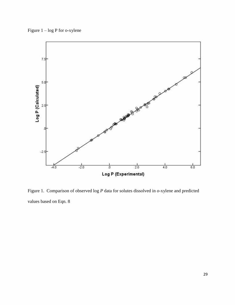
We have assembled in Table 1 log K and log P values for the partitioning of 59 solutes
between the gas phase and o-xylene, and between water and o-xylene at 298 K. The solutes
Page 7
7
considered cover a reasonably wide range of compound type and descriptor values. Preliminary
analysis of the experimental log K data yielded a correlation equation having very small bk
coefficients, would be expected from the molecular structure considerations. o-Xylene does not
have an acidic hydrogen. The bk-coefficients were set equal to zero, and the final regression
analyses performed to give:
log P = 0.083(0.041) + 0.518(0.065) E – 0.813(0.087) S – 2.884(0.064) A – 4.821(0.121) B
+ 4.559(0.082) V (8)
(N = 59, SD = 0.104, R2 = 0.997, F = 3055)
and
log K = 0.064(0.027) – 0.296(0.070) E + 0.934(0.092) S + 0.647(0.069) A + 1.010(0.019) L
(9)
(N = 59, SD = 0.120, R2
= 0.998, F = 8943)
All regression analyses were performed using SPSS statistical software. The standard errors in
the calculated coefficients are given in parenthesis. Here and elsewhere, N corresponds to the
number of solutes, R denotes the correlation coefficient, SD is the standard deviation and F
corresponds to the Fisher F-statistic. The statistics of both correlations are quite good as
evidenced by the near unity values of the squared correlation coefficients and by the small
standard deviations of SD = 0.104 and SD = 0.120 log units. The maximum deviation between
the observed and predicted values was 0.40 log units for both the log P (for iodine) and the log K
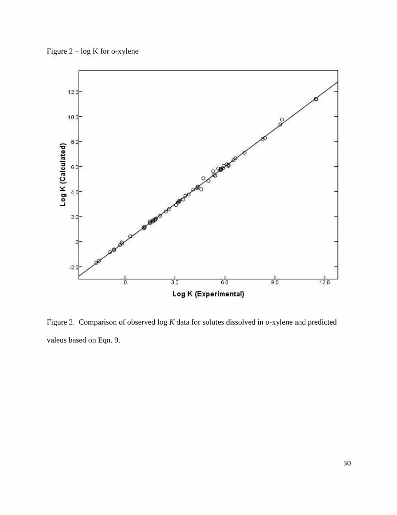
(for iodine) correlations. See Figures 1 and 2 for plots of the calculated log P and log K values
based on Eqns. 8 and 9 against observed data. The experimental log P and log K values cover
ranges of about 8.2 and 12.5 log units, respectively.
Page 8
8
The predictive ability of Eqns. 8 and 9 was assessed through a training set and test
analysis. The parent data points were divided into three subsets (A–C) as follows: the 1st, 4th,
7th, etc. data points comprise the first subset (A); the 2nd, 5th, 8th, etc. data points comprise the
second subset (B); the 3rd, 6th, 9th, etc. data points comprise the third subset (C). Three training
sets were prepared as combinations of two subsets (A and B), (A and C), and (B and C). Each
validation computation gave a training set correlation equation having coefficients not too
different from that obtained from the parent 59 compound database. The training set equations
were then used to predict log P and log K values for the compounds in the respective test sets
(A–C). The statistical information for the three test set predictions are summarized in Table 3.
For the three test sets the average values of S.D. = 0.116, AAE (average absolute error) = 0.083,
and AE (average error) = 0.003 were obtained for the water-to-o-xylene log P correlation, and
average values of S.D. = 0.119, AAE = 0.080, and AE = 0.013 were obtained for the gas-to-o-
xylene log K correlation. We conclude that there is very little bias in the predictions based on the
derived Abraham model correlations, and that Eqs. 8 and 9 can be used to predict further values
with an S.D. of about 0.12 log units.
The predictive ability was further examined using the leave-one-out method. The first
data point was removed from the training data set and the correlation model was calibrated on
the remaining data points, which in the present case are 58 experimental values. The value for
the left-out data point was then predicted with the derived mathematical correlation, and the
deviation between the predicted and observed log P (or log K) was computed. The data point
was returned to data set, the second data point was removed, and the process repeated until every
experimental value had been removed once. The computed deviations were then averaged to
obtain an indication of the predictive ability of the respective log P and log K correlation models.
Page 9
9
Calculated average errors of AAE = 0.085 and AAE = 0.092 log units were obtained for the
respective log P and log K predictions.
The data set for m-xylene contains experimental log P and log K values for 79 organic
solutes and gases. Regression analysis of the tabulated experimental values in Table 2 gave the
following two mathematical expressions:
log P = 0.122(0.025) + 0.377(0.048) E – 0.603(0.070) S – 2.981(0.053) A – 4.961(0.064) B
+ 4.535(0.031) V (10)
(N = 79, SD = 0.120, R2 = 0.998, F = 7216)
and
log K = 0.071(0.023) – 0.423(0.038) E + 1.068(0.048) S + 0.552(0.055) A + 1.014(0.008) L
(11)
(N = 79, SD = 0.130, R2
= 0.999, F = 17946)
The bk coefficient in the log K correlation was found to be negligible, and was removed from the
final correlation. Both correlations provide a reasonably accurate mathematical description of
the experimental water-to-m-xylene partition coefficient data (Eqn. 10) and gas-to-m-xylene
partition coefficient data (Eqn. 11) for experimental values that cover ranges of about 20.4 and
21.7 log units, respectively. The maximum deviation between the observed and predicted
values was 0.48 log units for the log P correlation and 0.50 log units for the log K correlation.
The solute in both cases was iodine. Graphical comparisons of predicted versus observed values
are given in Figures S1 and S2 (Supporting Information).
In order to assess the predictive ability of Eqns. 10 and 11 we divided the data points
into a training set and a test set by allowing the SPSS software to randomly select half of the
experimental data points. The selected data points became the training sets and the remaining
Page 10
10
compounds that were left served as the test sets. Analysis of the experimental data in the log P
and log K training sets gave:
log P = 0.091(0.043) + 0.316(0.058) E – 0.596(0.104) S – 2.934(0.079) A – 5.015(0.096) B
+ 4.603(0.096) V (12)
(N = 40, SD = 0.100, R2 = 0.997, F = 266.8)
and
log K = 0.094(0.031) – 0.467(0.048) E + 1.063(0.098) S + 0.546(0.078) A + 1.012(0.023) L
(13)
(N = 40, SD = 0.115, R2
= 0.999, F = 7199)
There is very little difference in the equation coefficients for the full dataset and the training
dataset correlations, thus showing that both training sets of compounds are representative
samples of the total log P and log K data sets. The derived training set equations were then used
to predict the respective partition coefficients for the compounds in the test sets. For the
predicted and experimental values, we found SD = 0.147 (Eqn. 12) and SD = 0.153 (Eqn. 13),
AAE = 0.101 (Eqn. 12) and AAE = 0.098 (Eqn. 13), and AE = 0.019 (Eqn. 12) and AE = –0.023
(Eqn. 13). There is therefore very little bias in using Eqns. 12 and 13 with AE equal to 0.019 and
–0.023 log units. The training and test set analyses were performed five more times with similar
results.
In Table 3 are collected values of the logarithms of the partition coefficients of 91
organic solutes and gases in p-xylene. Regression analyses of the experimental log P and log K
data in accordance with the Abraham model yielded :
log P = 0.166(0.032) + 0.477(0.060) E – 0.812(0.094) S – 2.939(0.071) A – 4.874(0.096) B
+ 4.532(0.033) V (14)
Page 11
11
(N = 91, SD = 0.137, R2 = 0.997, F = 6720)
and
log K = 0.113(0.023) – 0.302(0.052) E + 0.826(0.070) S + 0.651(0.061) A + 1.011(0.007) L
(15)
(N = 91, SD = 0.120, R2
= 0.998, F = 10227)
The bk coefficient in the log K correlation was again found to be negligible, and was removed
from the final correlation. Both equations are statistically very good with standard deviations of
0.137 and 0.120 log units for data sets that cover ranges of about 21.0 and 15.8 log units,
respectively (See Figures S3 and S4 in the Supporting Information for a graphical comparison of
observed versus predicted values). The maximum deviation between the observed and predicted
values was 0.40 log units for the log P correlation (for iodine) and 0.40 log units for the log K
correlation (for iodine and vinyl acetylene). The robustness of each correlation was determined
through a training set and test set analyses as before by splitting the large data set in half. To
conserve journal space we give only the test results. The training set correlations predicted the
45 experimental log P values in the test set to within SD = 0.172, AAE = 0.130 and AE = 0.020,
and the 45 experimental log K values in the test set to within SD = 0.144, AAE = 0.096 and AE
= –0.010. The training and test set analyses were performed five more times with similar results.
The present study shows that the correlations derived from the Abraham solvation
parameter model provide reasonably accurate mathematical descriptions of solute transfer at 298
K from both water and from the gas phase into each of the three xylene isomers. The derived
correlations pertain to 298 K. Careful examination of the three sets of log P correlations and
three sets of log K correlations reveals that for each transfer process the equation coefficients are
nearly identical as would be expected from the very similar molecular structures. The location of
Page 12
12
the two methyl functional groups on the aromatic ring does not significantly affect the solvent’s
molecular interactions with dissolved solute molecules.
Page 13
13
References
[ 1] M.H. Abraham, A.M. Zissimos, W.E. Acree, Jr., New J. Chem. 27 (2003) 1041-1044.
[ 2] L.M. Sprunger, S.S. Achi, R. Pointer, W.E. Acree, Jr., M.H. Abraham, Fluid Phase
Equilibr. 288 (2010) 121-127.
[ 3] L.M. Sprunger, S.S. Achi, R. Pointer, B.H. Blake-Taylor, W.E. Acree, Jr., M.H.
Abraham, Fluid Phase Equilibr. 286 (2009) 170-174.
[ 4] M.H. Abraham, W.E. Acree, Jr., J.E. Cometto-Muniz, New J. Chem. 33 (2009) 2034-
2043.
[ 5] M.H. Abraham, W.E. Acree, Jr., A.J. Leo, D. Hoekman, New J. Chem. 33 (2009) 1685-
1692.
[ 6] L.M. Sprunger, S.S. Achi, W.E. Acree, Jr., M.H. Abraham, A.J. Leo, D. Hoekman,
Fluid Phase Equilibr. 281 (2009) 144-162.
[ 7] M.H. Abraham, W.E. Acree, Jr., A.J. Leo, D. Hoekman, New J. Chem. 33 (2009) 568-
573.
[ 8] L.M. Sprunger, J. Gibbs, W.E. Acree, Jr., M.H. Abraham, Fluid Phase Equilibr. 273
(2008) 78-86.
[ 9] M.H. Abraham, Chem. Soc. Rev. 23, 73-83 (1993).
[10] M.H. Abraham, A. Ibrahim, A.M. Zissimos, J. Chromatogr., A 1037 (2004) 29-47.
[11] M.H. Abraham, R.E. Smith, R. Luchtefeld, A.J. Boorem, R. Luo, W.E. Acree, Jr., J.
Pharm. Sci. 99 (2010) 1500-1515.
[12] M.H. Abraham, W.E. Acree, Jr., J. Phys. Org. Chem. 21 (2008) 823-832.
[13] L.M. Sprunger, A. Proctor, W.E. Acree, Jr., M.H. Abraham, N. Benjelloun-Dakhama,
Fluid Phase Equilibr. 270 (2008) 30-44.
Page 14
14
[14] M.H. Abraham, A. Nasezadeh, W.E. Acree, Jr., Ind. Eng. Chem. Res. 47 (2008) 3990-
3995.
[ 15] M.H. Abraham, C.E. Green, W.E. Acree, Jr., C.E. Hernandez, L.E. Roy, J. Chem. Soc.,
Perkin Trans. 2 (1998) 2677-2682.
[16] C.E. Green, M.H. Abraham, W.E. Acree, Jr., K.M. De Fina, T.L. Sharp, Pest Manage.
Sci. 56 (2000) 1043-1053.
[17] W.J. Cheong, P.W. Carr, J. Chromatogr. 500 (1990) 215-239.
[18] G. Kolasinska, M. Goral, J. Giza, Z. Phys. Chem. (Leipzig) 263 (1982) 151-160.
[19] R.P. Singh, S.S. Singh, J. Indian Chem. Soc. 54 (1977) 1035-1039.
[20] A.W. Shaw, A.J. Vosper, J. Chem. Soc., Faraday Trans. 1 73 (1977) 1239-1244.
[21] J.E. Byrne, R. Battino, E. Wilhelm, J. Chem. Thermodyn. 7 (1975) 515-522.
[22] A. Ignat, L. Molder, Eesti NSV Tead. Akad. Toim. Keem. 38 (1989) 11-16.
[23] E.R. Thomas, B.A. Newman, T.C. Long, D.A. Wood, C.A. Eckert, J. Chem. Eng. Data
27 (1982) 399-405.
[24] L. Rohrschneider, Anal. Chem. 45 (1973) 1241-1247.
[25] J.H. Park, A. Hussan, P. Couasnon, D. Fritz, P.W. Carr, Anal. Chem. 59 (1987) 1970-
1976.
[26] D. I. Eikens, Ph.D. Dissertation, University of Minnesota, Minneapolis, Minnesota
(1993).
[27] N.K. Naumenko, N.N. Mukhin, V.B. Aleskovskii, Zh. Prikl. Khim. 42 (1969) 2522-2528.
[28] C. Knoop, D. Tiegs, J. Gmehling, J. Chem. Eng. Data 34 (1989) 240-247.
[29] R.G. Linford, D.G.T. Thornhill, J. Appl. Chem. Biotechnol. 27 (1977) 479-497.
[30] T. Boublik, G.C. Benson, Can. J. Chem. 47 (1969) 539-542.
Page 15
15
[31] D.V.S. Jain, R.K. Wadi, J. Chem. Thermodyn. 8 (1976) 493-497.
[32] J. Gmehling, U. Onken, W. Arlt, Vapor-liquid Equilibrium Data Collection: Chemical
Data Series, Volume I, parts 2b-d, DECHEMA, Franfurt/Main, Germany (1978 – 1984).
[33] B.S. Mahl, J.R. Khurma, J.N. Vij, Thermochim. Acta 19 (1977) 124-128.
[34] B.S. Mahl, J.R. Khurma, J. Chem. Soc., Faraday Trans. 1 73 (1977) 29-31.
[35] K.N. Marsh, J.B. Ott, Int. DATA Ser., Sel. Data Mix., Ser. A (1884) 202-208.
[36] M. Goral, Fluid Phase Equilibr. 102 (1994) 275-286.
[37] J. Vitovec, V. Fried, Collect. Czech. Chem. Comm. 25 (1960) 2218-2222.
[38] J. Vitovec, V. Fried, Collect. Czech. Chem. Comm. 25 (1960) 1552-1556.
[39] S.M. Ashraf, D.H.L. Prasad, Phys. Chem. Liq. 38 (2000) 381-390.
[40] R. Tanaka, G.C. Benson, J. Chem. Eng. Data 21 (1976) 320-324.
[41] P. Oracz, Int. DATA Ser. Sel. Data Mix., Ser. A (1989) 250-252.
[42] U. Bhardwaj, K.C. Sing, S. Maken, J. Chem. Thermodyn. 30 (1998) 253-261.
[43] Y. Miyano, A. Kimura, M. Kuroda, A. Matsushita, A. Yamasaki, Y. Yamaguchi, A.
Yoshizawa, Y. Tateishi, J. Chem. Eng. Data 52 (2007) 291-297.
[44] M. Lohse, W.-D. Deckwer, J. Chem. Eng. Data 26 (1981) 159-161.
[45] M.-C. Haulait-Pirson, G. Huys, E. Vanstraelen, Ind. Eng. Chem. Fundam. 26 (1987) 447-
452.
[46] C.-Z. Jiang, F._J. Hsu, V. Fried, J. Chem. Eng. Data 28 (1983) 75-78.
[47] K.A. Fletcher, K.S. Coym, L.E. Roy, C.E. Hernandez, M.E.R. McHale, W.E. Acree, Jr.,
Phys. Chem. Liq. 35 (1998) 243-252.
[48] W.E. Acree, Jr., S.A. Tucker, Phys. Chem. Liq. 20 (1989) 31-38.
Page 16
16
[49] L.E. Roy, C.E. Hernandez, W.E. Acree, Jr., Polycyclic Aromat. Compds. 13 (1999) 105-
116.
[50] L.E. Roy, C.E. Hernandez, K.M. De Fina, W.E. Acree, Jr., Phys. Chem. Liq. 38 (2000)
333-343.
[51] J.R. Powell, D. Voisinet, A. Salazar, W.E. Acree, Jr., Phys. Chem. Liq. 28 (1994) 269-
276.
[52] K.M. De Fina, C. Ezell, W.E. Acree, Jr., Phys. Chem. Liq. 39 (2001) 699-710.
[53] V.M. Kravchenko, I.S. Pastukhova, Zhur. Fiz. Khim. 31 (1957) 1802-1811.
[54] V.M. Kravchenko, Zhur. Priklad. Khim. 22 (1949) 724-733.
[55] A. Jacob, R. Joh, C. Rose, J. Gmehling, Fluid Phase Equilibr. 113 (1995) 117-126.
[56] V.M. Kravchenko, Zhur. Fiz. Khim. 13 (1939) 989-1000.
[57] D.H.M. Beiny, J.W. Mullin, J. Chem. Eng. Data 32, 9-10 (1987).
[58] W. Bobak, W. Apostoluk, P. Maciejewski, Anal. Chim. Acta 569 (2006) 119-131.
[59] I.E. Dobryakova, Yu. G. Dobryakov, Russ. J. Appl. Chem. 77 (2004) 1750-1753.
[60] Ya. I. Korenman, Zhur. Priklad. Khim. 47 (1974) 2079-2083.
[61] Ya. I. Korenman, Russ. J. Phys. Chem. 46 (1972) 334-336.
[62] Ya.I. Korenman, T.V. Makarova, Zhur. Priklad. Khim. 47 (1974) 1624-1628.
[63] W. Kemula, H. Buchowski, J. Terperek, Bull. L’Acad. Polon. Sci. 12 (1964) 347-349.
[64] Ya. I. Korenman, Russ. J. Phys. Chem. 46 (1972) 1286-1288.
[65] I.M. Korenman, T.M. Kochetkova, Trudy po Khim. Khimicheskoi Tekhnol. (1968) 110-
116.
[66] J. Arro, L. Molder, Russ. J. Phys. Chem. 49 (1975) 635-636.
[67] Ya. I. Korenman, T.P. Koroleva, Zhur. Priklad. Khim. 48 (1975) 1413-1415.
Page 17
17
[68] I. M. Korenman, B.A. Nikolaev, T.A. Bogomolova, Zhur. Priklad. Khim. 48 (1975) 664-
666.
[69] Ya. I. Korenman, A.A. Gorokhov, Russ. J. Phys. Chem. 47 (1973) 1157-1158.
[70] M. Goral, B. Wisniewska, A. Maczynski, J. Phys. Chem. Data 33 (2004) 1159-1188.
Page 18
18
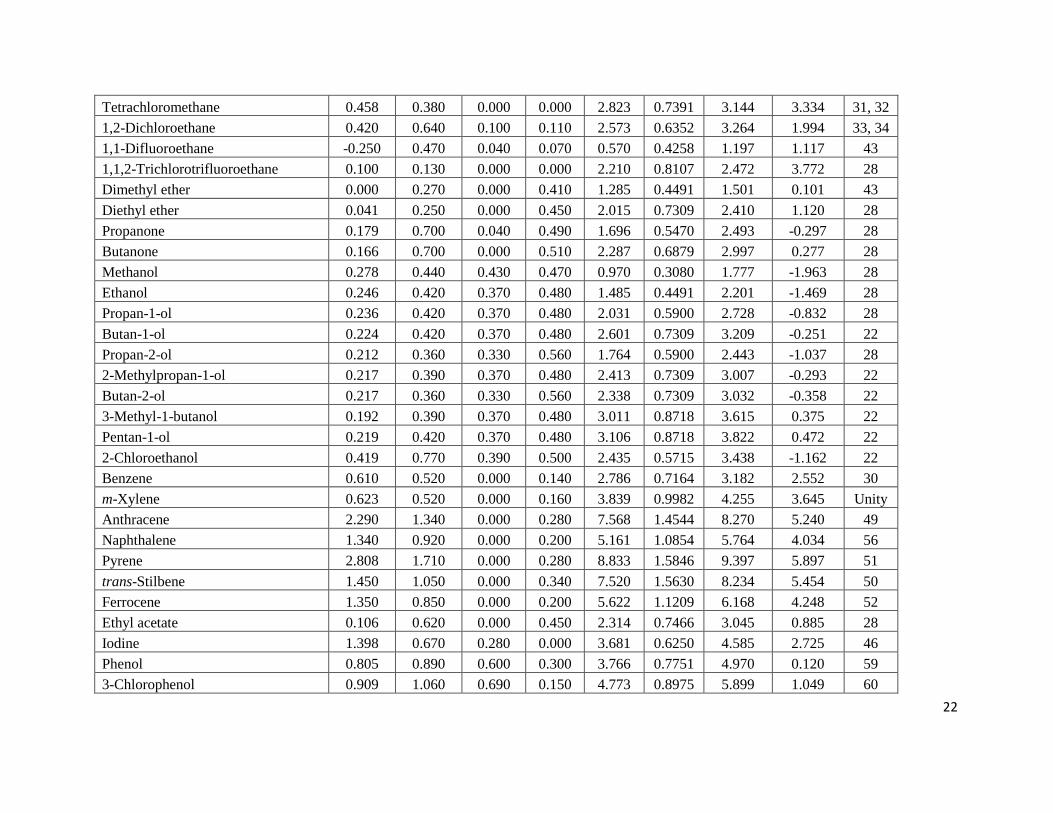
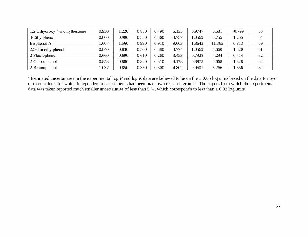
Table 1. Experimental log Pa and log K
a Data for Solutes Dissolved in o-Xylene at 298 K
Solute E S A B L V Log Kobs Log Pobs Ref
Helium 0.000 0.000 0.000 0.000 -1.741 0.0680 -1.735 0.295 21
Neon 0.000 0.000 0.000 0.000 -1.575 0.0850 -1.564 0.396 21
Argon 0.000 0.000 0.000 0.000 -0.688 0.1900 -0.660 0.810 21
Krypton 0.000 0.000 0.000 0.000 -0.211 0.2460 -0.165 1.045 21
Oxygen 0.000 0.000 0.000 0.000 -0.723 0.1830 -0.646 0.864 27
Carbon dioxide 0.000 0.280 0.050 0.100 0.058 0.2809 0.314 0.394 21
Tetrafluoromethane -0.580 -0.260 0.000 0.000 -0.817 0.3203 -0.888 1.402 21
Sulfur hexaflouride -0.600 -0.200 0.000 0.000 -0.120 0.4643 -0.200 2.020 21
Methane 0.000 0.000 0.000 0.000 -0.323 0.2495 -0.294 1.166 21
Propane 0.000 0.000 0.000 0.000 1.050 0.5313 1.116 2.556 43
Butane 0.000 0.000 0.000 0.000 1.615 0.6722 1.692 3.212 43
2-Methylpropane 0.000 0.000 0.000 0.000 1.409 0.6722 1.495 3.195 43
1-Propene 0.100 0.080 0.000 0.070 0.946 0.4883 1.144 2.114 43
1-Butene 0.100 0.080 0.000 0.070 1.491 0.6292 1.695 2.705 43
cis 2-Butene 0.140 0.080 0.000 0.050 1.737 0.6292 1.863 2.853 43
trans 2-Butene 0.126 0.080 0.000 0.050 1.664 0.6292 1.812 2.792 43
2-Methylprop-1-ene 0.120 0.080 0.000 0.080 1.579 0.6292 1.692 2.552 43
1,3-Butadiene 0.320 0.230 0.000 0.100 1.543 0.5862 1.805 2.255 43
Chloroethane 0.227 0.400 0.000 0.100 1.678 0.5128 2.099 1.639 43
Dichloromethane 0.390 0.570 0.100 0.050 2.019 0.4943 2.627 1.667 19
Tetrachloromethane 0.458 0.380 0.000 0.000 2.823 0.7391 3.183 3.373 31, 32
1,2-Dichloroethane 0.420 0.640 0.100 0.110 2.573 0.6352 3.238 1.964 33, 34
1,1-Difluoroethane -0.250 0.470 0.040 0.070 0.570 0.4258 1.186 1.106 43
Dimethyl ether 0.000 0.270 0.000 0.410 1.285 0.4491 1.493 0.093 43
Propanone 0.179 0.700 0.040 0.490 1.696 0.5470 2.460 -0.330 18
Page 19
19
Butan-1-ol 0.224 0.420 0.370 0.480 2.601 0.7309 3.272 -0.188 22
Butan-2-ol 0.217 0.360 0.330 0.560 2.338 0.7309 3.068 -0.322 22
3-Methyl-1-butanol 0.192 0.390 0.370 0.480 3.011 0.8718 3.621 0.381 22
Pentan-1-ol 0.219 0.420 0.370 0.480 3.106 0.8718 3.816 0.466 22
Hexan-1-ol 0.210 0.420 0.370 0.480 3.610 1.0127 4.332 1.102 22
2-Chloroethanol 0.419 0.770 0.390 0.500 2.435 0.5715 3.474 -1.260 22
o-Xylene 0.663 0.560 0.000 0.160 3.939 0.9982 4.363 3.623 Unity
Chlorobenzene 0.718 0.650 0.000 0.070 3.657 0.8388 4.098 3.278 39, 40
Anthracene 2.290 1.340 0.000 0.280 7.568 1.4544 8.406 5.376 49
Naphthalene 1.340 0.920 0.000 0.200 5.161 1.0854 5.757 4.027 54
Acenaphthene 1.604 1.050 0.000 0.220 6.469 1.2586 7.171 4.811 53
Pyrene 2.808 1.710 0.000 0.280 8.833 1.5846 9.428 5.928 51
trans-Stilbene 1.450 1.050 0.000 0.340 7.520 1.5630 8.265 5.485 50
Ferrocene 1.350 0.850 0.000 0.200 5.622 1.1209 6.207 4.287 52
Iodine 1.398 0.670 0.280 0.000 3.681 0.6250 4.570 2.710 46
Phenol 0.805 0.890 0.600 0.300 3.766 0.7751 5.017 0.167 59
3-Chlorophenol 0.909 1.060 0.690 0.150 4.773 0.8975 5.918 1.068 60
4-Chlorophenol 0.915 1.080 0.670 0.200 4.775 0.8975 6.213 1.053 60
2,4-Dichlorophenol 0.960 0.820 0.540 0.170 4.896 1.0199 5.601 1.951 60
Thioxanthen-9-one 1.940 1.441 0.000 0.557 8.436 1.5357 9.325 4.257 47
Chlorine 0.360 0.320 0.100 0.000 1.193 0.3534 1.527 1.347 44
2-Methylaniline 0.966 0.920 0.230 0.450 4.442 0.9571 5.418 1.358 65
4-Methylaniline 0.923 0.950 0.230 0.450 4.452 0.9571 5.331 1.241 65
Resorcinol 0.980 1.110 1.090 0.520 4.618 0.8338 6.103 -2.247 66
Catechol 0.970 1.100 0.880 0.470 4.450 0.8338 5.879 -1.321 66
Hydroquinone 1.063 1.270 1.060 0.570 4.827 0.8338 6.511 -2.359 66
Benzidine 1.882 2.450 0.400 0.800 9.230 1.5238 11.483 1.053 68
Page 20
20
1,2-Dihydroxy-4-methylbenzene 0.950 1.220 0.850 0.490 5.135 0.9747 6.632 -0.798 66
4-Ethylphenol 0.800 0.900 0.550 0.360 4.737 1.0569 5.772 1.272 64
Bisphenol A 1.607 1.560 0.990 0.910 9.603 1.8643 11.458 0.908 69
2,5-Dimethylphenol 0.840 0.830 0.500 0.380 4.774 1.0569 5.720 1.380 61
2-Fluorophenol 0.660 0.690 0.610 0.260 3.453 0.7928 4.371 0.491 62
2-Chlorophenol 0.853 0.880 0.320 0.310 4.178 0.8975 4.702 1.352 62
2-Bromophenol 1.037 0.850 0.350 0.300 4.802 0.9501 5.290 1.580 62
a Estimated uncertainties in the experimental log P and log K data are believed to be on the ± 0.05 log units based on the data for two
or three solutes for which independent measurements had been made two research groups. The papers from which the experimental
data was taken reported much smaller uncertainties of less than 5 %, which corresponds to less than ± 0.02 log units.
Page 21
21
Table 2. Experimental log Pa and log K
a Data for Solutes Dissolved in m-Xylene at 298 K
Solute E S A B L V Log Kobs Log Pobs Ref
Helium 0.000 0.000 0.000 0.000 -1.741 0.0680 -1.690 0.330 21
Neon 0.000 0.000 0.000 0.000 -1.575 0.0850 -1.485 0.475 21
Argon 0.000 0.000 0.000 0.000 -0.688 0.1900 -0.628 0.842 21
Krypton 0.000 0.000 0.000 0.000 -0.211 0.2460 -0.142 1.068 21
Hydrogen 0.000 0.000 0.000 0.000 -1.200 0.1086 -1.089 0.631 21
Oxygen 0.000 0.000 0.000 0.000 -0.723 0.1830 -0.624 0.886 27
Nitric Oxide 0.370 0.020 0.000 0.086 -0.590 0.2026 -0.580 0.747 20
Carbon dioxide 0.000 0.280 0.050 0.100 0.058 0.2809 0.328 0.408 21
Tetrafluoromethane -0.580 -0.260 0.000 0.000 -0.817 0.3203 -0.827 1.461 21
Sulfur hexaflouride -0.600 -0.200 0.000 0.000 -0.120 0.4643 -0.142 2.078 21
Methane 0.000 0.000 0.000 0.000 -0.323 0.2495 -0.269 1.191 21
Propane 0.000 0.000 0.000 0.000 1.050 0.5313 1.190 2.630 43
Butane 0.000 0.000 0.000 0.000 1.615 0.6722 1.713 3.233 43
2-Methylpropane 0.000 0.000 0.000 0.000 1.409 0.6722 1.518 3.218 43
Pentane 0.000 0.000 0.000 0.000 2.162 0.8131 2.279 3.979 28
Hexane 0.000 0.000 0.000 0.000 2.668 0.9540 2.821 4.641 28
Octacosane 0.000 0.000 0.000 0.000 13.780 4.0536 14.109 18.449 57
Ethene 0.107 0.100 0.000 0.070 0.289 0.3470 0.447 1.387 29
1-Propene 0.100 0.080 0.000 0.070 0.946 0.4883 1.158 2.128 43
1-Butene 0.100 0.080 0.000 0.070 1.491 0.6292 1.688 2.698 43
cis 2-Butene 0.140 0.080 0.000 0.050 1.737 0.6292 1.881 2.871 43
trans 2-Butene 0.126 0.080 0.000 0.050 1.664 0.6292 1.829 2.809 43
2-Methylprop-1-ene 0.120 0.080 0.000 0.080 1.579 0.6292 1.709 2.569 43
1,3-Butadiene 0.320 0.230 0.000 0.100 1.543 0.5862 1.815 2.265 43
1-Hexene 0.078 0.080 0.000 0.070 2.572 0.9110 2.738 3.898 28
Chloroethane 0.227 0.400 0.000 0.100 1.678 0.5128 2.106 1.646 43
Dichloromethane 0.390 0.570 0.100 0.050 2.019 0.4943 2.624 1.664 28
Page 22
22
Tetrachloromethane 0.458 0.380 0.000 0.000 2.823 0.7391 3.144 3.334 31, 32
1,2-Dichloroethane 0.420 0.640 0.100 0.110 2.573 0.6352 3.264 1.994 33, 34
1,1-Difluoroethane -0.250 0.470 0.040 0.070 0.570 0.4258 1.197 1.117 43
1,1,2-Trichlorotrifluoroethane 0.100 0.130 0.000 0.000 2.210 0.8107 2.472 3.772 28
Dimethyl ether 0.000 0.270 0.000 0.410 1.285 0.4491 1.501 0.101 43
Diethyl ether 0.041 0.250 0.000 0.450 2.015 0.7309 2.410 1.120 28
Propanone 0.179 0.700 0.040 0.490 1.696 0.5470 2.493 -0.297 28
Butanone 0.166 0.700 0.000 0.510 2.287 0.6879 2.997 0.277 28
Methanol 0.278 0.440 0.430 0.470 0.970 0.3080 1.777 -1.963 28
Ethanol 0.246 0.420 0.370 0.480 1.485 0.4491 2.201 -1.469 28
Propan-1-ol 0.236 0.420 0.370 0.480 2.031 0.5900 2.728 -0.832 28
Butan-1-ol 0.224 0.420 0.370 0.480 2.601 0.7309 3.209 -0.251 22
Propan-2-ol 0.212 0.360 0.330 0.560 1.764 0.5900 2.443 -1.037 28
2-Methylpropan-1-ol 0.217 0.390 0.370 0.480 2.413 0.7309 3.007 -0.293 22
Butan-2-ol 0.217 0.360 0.330 0.560 2.338 0.7309 3.032 -0.358 22
3-Methyl-1-butanol 0.192 0.390 0.370 0.480 3.011 0.8718 3.615 0.375 22
Pentan-1-ol 0.219 0.420 0.370 0.480 3.106 0.8718 3.822 0.472 22
2-Chloroethanol 0.419 0.770 0.390 0.500 2.435 0.5715 3.438 -1.162 22
Benzene 0.610 0.520 0.000 0.140 2.786 0.7164 3.182 2.552 30
m-Xylene 0.623 0.520 0.000 0.160 3.839 0.9982 4.255 3.645 Unity
Anthracene 2.290 1.340 0.000 0.280 7.568 1.4544 8.270 5.240 49
Naphthalene 1.340 0.920 0.000 0.200 5.161 1.0854 5.764 4.034 56
Pyrene 2.808 1.710 0.000 0.280 8.833 1.5846 9.397 5.897 51
trans-Stilbene 1.450 1.050 0.000 0.340 7.520 1.5630 8.234 5.454 50
Ferrocene 1.350 0.850 0.000 0.200 5.622 1.1209 6.168 4.248 52
Ethyl acetate 0.106 0.620 0.000 0.450 2.314 0.7466 3.045 0.885 28
Iodine 1.398 0.670 0.280 0.000 3.681 0.6250 4.585 2.725 46
Phenol 0.805 0.890 0.600 0.300 3.766 0.7751 4.970 0.120 59
3-Chlorophenol 0.909 1.060 0.690 0.150 4.773 0.8975 5.899 1.049 60
Page 23
23
4-Chlorophenol 0.915 1.080 0.670 0.200 4.775 0.8975 6.151 0.991 60
2,4-Dichlorophenol 0.960 0.820 0.540 0.170 4.896 1.0199 5.540 1.890 60
Thioxanthen-9-one 1.940 1.441 0.000 0.557 8.436 1.5357 9.258 4.190 47
15-Crown-5 0.410 1.200 0.000 1.750 6.779 1.7025 8.030 -1.370 58
16-Crown-5 0.410 1.170 0.000 1.760 7.276 1.8434 8.390 -0.790 58
Benzo 15-Crown-5 1.055 1.940 0.000 1.590 9.403 2.0285 10.850 0.300 58
18-Crown-6 0.410 1.470 0.000 2.100 8.228 2.0430 9.480 -1.950 58
Dibenzo-18-Crown-6 1.690 2.730 0.000 1.780 13.384 2.6950 15.930 2.550 58
Dibenzo-24-Crown-8 1.680 3.400 0.000 2.340 16.414 3.3760 19.990 2.610 58
AC-Benzo-18-Crown-6 0.684 2.650 0.000 1.850 11.100 2.4776 14.056 1.006 58
2-Methylaniline 0.966 0.920 0.230 0.450 4.442 0.9571 5.367 1.307 65
4-Methylaniline 0.923 0.950 0.230 0.450 4.452 0.9571 5.323 1.233 65
Resorcinol 0.980 1.110 1.090 0.520 4.618 0.8338 6.104 -2.246 66
Catechol 0.970 1.100 0.880 0.470 4.450 0.8338 5.842 -1.358 66
Hydroquinone 1.063 1.270 1.060 0.570 4.827 0.8338 6.512 -2.538 66
1,2-Dihydroxy-4-methylbenzene 0.950 1.220 0.850 0.490 5.135 0.9747 6.633 -0.797 66
4-Ethylphenol 0.800 0.900 0.550 0.360 4.737 1.0569 5.743 1.243 64
Bisphenol A 1.607 1.560 0.990 0.910 9.603 1.8643 11.395 0.845 69
2,5-Dimethylphenol 0.840 0.830 0.500 0.380 4.774 1.0569 5.690 1.350 61
2-Nitrophenol 1.015 1.050 0.050 0.370 4.760 0.9493 5.663 2.303 63
2-Fluorophenol 0.660 0.690 0.610 0.260 3.453 0.7928 4.319 0.439 62
2-Chlorophenol 0.853 0.880 0.320 0.310 4.178 0.8975 4.709 1.369 62
2-Bromophenol 1.037 0.850 0.350 0.300 4.802 0.9501 5.330 1.620 62
a Estimated uncertainties in the experimental log P and log K data are believed to be on the ± 0.05 log units based on the data for two
or three solutes for which independent measurements had been made two research groups. The papers from which the experimental
data was taken reported much smaller uncertainties of less than 5 %, which corresponds to less than ± 0.02 log units.
Page 24
24
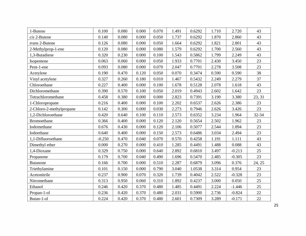
Table 3. Experimental log Pa and log K
a Data for Solutes Dissolved in p-Xylene at 298 K
Solute E S A B L V Log Kobs Log Pobs Ref
Helium 0.000 0.000 0.000 0.000 -1.741 0.0680 -1.674 0.346 21
Neon 0.000 0.000 0.000 0.000 -1.575 0.0850 -1.521 0.439 21
Argon 0.000 0.000 0.000 0.000 -0.688 0.1900 -0.608 0.862 21
Krypton 0.000 0.000 0.000 0.000 -0.211 0.2460 -0.125 1.085 21
Oxygen 0.000 0.000 0.000 0.000 -0.723 0.1830 -0.609 0.901 27
Carbon dioxide 0.000 0.280 0.050 0.100 0.058 0.2809 0.332 0.340 21
Tetrafluoromethane -0.580 -0.260 0.000 0.000 -0.817 0.3203 -0.814 1.476 21
Sulfur hexaflouride -0.600 -0.200 0.000 0.000 -0.120 0.4643 -0.141 2.079 21
Methane 0.000 0.000 0.000 0.000 -0.323 0.2495 -0.244 1.216 21
Propane 0.000 0.000 0.000 0.000 1.050 0.5313 1.146 2.586 43
Butane 0.000 0.000 0.000 0.000 1.615 0.6722 1.709 3.229 43
2-Methylpropane 0.000 0.000 0.000 0.000 1.409 0.6722 1.509 3.209 43
Pentane 0.000 0.000 0.000 0.000 2.162 0.8131 2.303 4.003 23, 26
Hexane 0.000 0.000 0.000 0.000 2.668 0.9540 2.818 4.638 26
Heptane 0.000 0.000 0.000 0.000 3.173 1.0949 3.336 5.296 26
Octane 0.000 0.000 0.000 0.000 3.677 1.2358 3.839 5.949 24, 25, 26
Nonane 0.000 0.000 0.000 0.000 4.182 1.3767 4.329 6.479 26
Decane 0.000 0.000 0.000 0.000 4.686 1.5176 4.897 7.219 36
Octacosane 0.000 0.000 0.000 0.000 13.780 4.0536 14.167 18.507 58
2-Methylpentane 0.000 0.000 0.000 0.000 2.503 0.9540 2.651 4.801 26
2,4-Dimethylpentane 0.000 0.000 0.000 0.000 2.809 1.0949 2.962 5.042 26
2,5-Dimethylhexane 0.000 0.000 0.000 0.000 3.308 1.2358 3.472 5.492 26
2,3,4-Trimethylpentane 0.000 0.000 0.000 0.000 3.481 1.2358 3.541 5.421 26
Cyclohexane 0.305 0.100 0.000 0.000 2.964 0.8454 3.062 3.962 26
Ethylcyclohexane 0.263 0.100 0.000 0.000 3.877 1.1272 3.901 5.481 26
1-Propene 0.100 0.080 0.000 0.070 0.946 0.4883 1.161 2.131 43
Page 25
25
1-Butene 0.100 0.080 0.000 0.070 1.491 0.6292 1.710 2.720 43
cis 2-Butene 0.140 0.080 0.000 0.050 1.737 0.6292 1.870 2.860 43
trans 2-Butene 0.126 0.080 0.000 0.050 1.664 0.6292 1.821 2.801 43
2-Methylprop-1-ene 0.120 0.080 0.000 0.080 1.579 0.6292 1.700 2.560 43
1,3-Butadiene 0.320 0.230 0.000 0.100 1.543 0.5862 1.799 2.249 43
Isopentene 0.063 0.060 0.000 0.050 1.933 0.7701 2.430 3.450 23
Pent-1-ene 0.093 0.080 0.000 0.070 2.047 0.7701 2.278 3.508 23
Acetylene 0.190 0.470 0.120 0.050 0.070 0.3474 0.590 0.590 38
Vinyl acetylene 0.327 0.260 0.180 0.010 1.467 0.5432 2.249 2.279 37
Chloroethane 0.227 0.400 0.000 0.100 1.678 0.5128 2.078 1.618 43
Dichloromethane 0.390 0.570 0.100 0.050 2.019 0.4943 2.602 1.642 23
Tetrachloromethane 0.458 0.380 0.000 0.000 2.823 0.7391 3.190 3.380 23, 31
1-Chloropropane 0.216 0.400 0.000 0.100 2.202 0.6537 2.626 2.386 23
2-Chloro-2-methylpropane 0.142 0.300 0.000 0.030 2.273 0.7946 2.626 3.426 23
1,2-Dichloroethane 0.420 0.640 0.100 0.110 2.573 0.6352 3.234 1.964 32-34
Bromoethane 0.366 0.400 0.000 0.120 2.120 0.5654 2.502 1.962 23
Iodomethane 0.676 0.430 0.000 0.120 2.106 0.5077 2.544 1.894 23
Iodoethane 0.640 0.400 0.000 0.150 2.573 0.6486 3.034 2.494 23
1,1-Difluoroethane -0.250 0.470 0.040 0.070 0.570 0.4258 1.191 1.111 43
Dimethyl ether 0.000 0.270 0.000 0.410 1.285 0.4491 1.488 0.088 43
1,4-Dioxane 0.329 0.750 0.000 0.640 2.892 0.6810 3.497 -0.213 25
Propanone 0.179 0.700 0.040 0.490 1.696 0.5470 2.485 -0.305 23
Butanone 0.166 0.700 0.000 0.510 2.287 0.6879 3.096 0.376 24, 25
Triethylamine 0.101 0.150 0.000 0.790 3.040 1.0538 3.314 0.954 23
Acetonitrile 0.237 0.900 0.070 0.320 1.739 0.4042 2.522 -0.328 23
Nitromethane 0.313 0.950 0.060 0.310 1.892 0.4237 3.000 0.050 25
Ethanol 0.246 0.420 0.370 0.480 1.485 0.4491 2.224 -1.446 25
Propan-1-ol 0.236 0.420 0.370 0.480 2.031 0.5900 2.736 -0.824 22
Butan-1-ol 0.224 0.420 0.370 0.480 2.601 0.7309 3.289 -0.171 22
Page 26
26
Propan-2-ol 0.212 0.360 0.330 0.560 1.764 0.5900 2.486 -0.994 22
2-Methylpropan-1-ol 0.217 0.390 0.370 0.480 2.413 0.7309 3.115 -0.185 22
Butan-2-ol 0.217 0.360 0.330 0.560 2.338 0.7309 3.104 -0.286 22
2-Methylpropan-2-ol 0.180 0.300 0.310 0.600 1.963 0.7309 2.466 -0.814 41, 42
3-Methyl-1-butanol 0.192 0.390 0.370 0.480 3.011 0.8718 3.612 0.372 22
2-Chloroethanol 0.419 0.770 0.390 0.500 2.435 0.5715 3.496 -1.104 22
Carbon disulfide 0.876 0.260 0.000 0.030 2.370 0.4905 2.600 2.750 23
Benzene 0.610 0.520 0.000 0.140 2.786 0.7164 3.200 2.570 23, 35
Toluene 0.601 0.520 0.000 0.140 3.325 0.8573 3.735 3.085 25
p-Xylene 0.613 0.520 0.000 0.160 3.839 0.9982 4.233 3.643 Unity
Chlorobenzene 0.718 0.650 0.000 0.070 3.657 0.8388 4.050 3.230 39, 40
Anthracene 2.290 1.340 0.000 0.280 7.568 1.4544 8.231 5.201 48
Naphthalene 1.340 0.920 0.000 0.200 5.161 1.0854 5.778 4.048 54
Acenaphthene 1.604 1.050 0.000 0.220 6.469 1.2586 7.015 4.655 55
Pyrene 2.808 1.710 0.000 0.280 8.833 1.5846 9.381 5.881 51
trans-Stilbene 1.450 1.050 0.000 0.340 7.520 1.5630 8.279 5.499 50
Ferrocene 1.350 0.850 0.000 0.200 5.622 1.1209 6.185 4.265 52
Ethyl acetate 0.106 0.620 0.000 0.450 2.314 0.7466 3.083 0.923 23
Iodine 1.398 0.670 0.280 0.000 3.681 0.6250 4.551 2.691 46
Phenol 0.805 0.890 0.600 0.300 3.766 0.7751 4.960 0.110 59
3-Chlorophenol 0.909 1.060 0.690 0.150 4.773 0.8975 5.845 0.995 60
4-Chlorophenol 0.915 1.080 0.670 0.200 4.775 0.8975 6.079 0.919 60
2,4-Dichlorophenol 0.960 0.820 0.540 0.170 4.896 1.0199 5.555 1.905 64
Thioxanthen-9-one 1.940 1.441 0.000 0.557 8.436 1.5357 9.248 4.180 47
Chlorine 0.360 0.320 0.100 0.000 1.193 0.3534 1.535 1.355 44
Methyl 2-hydroxybenzoate 0.850 0.820 0.010 0.480 4.961 1.1313 5.601 2.631 67
Resorcinol 0.980 1.110 1.090 0.520 4.618 0.8338 6.118 -2.232 66
Catechol 0.970 1.100 0.880 0.470 4.450 0.8338 5.831 -1.369 66
Hydroquinone 1.063 1.270 1.060 0.570 4.827 0.8338 6.458 -2.412 66
Page 27
27
1,2-Dihydroxy-4-methylbenzene 0.950 1.220 0.850 0.490 5.135 0.9747 6.631 -0.799 66
4-Ethylphenol 0.800 0.900 0.550 0.360 4.737 1.0569 5.755 1.255 64
Bisphenol A 1.607 1.560 0.990 0.910 9.603 1.8643 11.363 0.813 69
2,5-Dimethylphenol 0.840 0.830 0.500 0.380 4.774 1.0569 5.660 1.320 61
2-Fluorophenol 0.660 0.690 0.610 0.260 3.453 0.7928 4.294 0.414 62
2-Chlorophenol 0.853 0.880 0.320 0.310 4.178 0.8975 4.668 1.328 62
2-Bromophenol 1.037 0.850 0.350 0.300 4.802 0.9501 5.266 1.556 62
a Estimated uncertainties in the experimental log P and log K data are believed to be on the ± 0.05 log units based on the data for two
or three solutes for which independent measurements had been made two research groups. The papers from which the experimental
data was taken reported much smaller uncertainties of less than 5 %, which corresponds to less than ± 0.02 log units.
Page 28
28
Table 4. Summary of Training Set and Test Set Computations for o-Xylene
______________________________________________________________________________
Predictions (log units)
Training Set Test Set S.D. AAE AE
______________________________________________________________________________
log P correlation
A + B C 0.098 0.080 0.017
A + C B 0.097 0.066 –0.028
B + C A 0.152 0.103 0.021
Average 0.116 0.083 0.003
log K correlation
A + B C 0.079 0.061 –0.001
A + C B 0.118 0.073 0.018
B + C A 0.160 0.105 0.022
Average 0.119 0.080 0.013
Page 29
29
Figure 1 – log P for o-xylene
Figure 1. Comparison of observed log P data for solutes dissolved in o-xylene and predicted
values based on Eqn. 8
Page 30
30
Figure 2 – log K for o-xylene
Figure 2. Comparison of observed log K data for solutes dissolved in o-xylene and predicted
valeus based on Eqn. 9.