Page 1
On 1D, N = 4 Supersymmetric SYK-Type Models (II)
S. James Gates, Jr.1 ,a,b, Yangrui Hu2 ,a,b, and S.-N. Hazel Mak3 ,a,b
aBrown Theoretical Physics Center,
Box S, 340 Brook Street, Barus Hall, Providence, RI 02912, USA
and
bDepartment of Physics, Brown University,
Box 1843, 182 Hope Street, Barus & Holley, Providence, RI 02912, USA
ABSTRACT
This paper is an extension of our last 1D, N = 4 supersymmetric SYK pa-per [arXiv:2103.11899]. In this paper we introduced the complex linear super-multiplet (CLS), which is “usefully inequivalent” to the chiral supermultiplet.We construct three types of models based on the complex linear supermultipletcontaining quartic interactions from modified CLS kinetic term, quartic inter-actions from 3-pt vertices integrated over the whole superspace, and 2(q−1)-ptinteractions generated via superpotentials respectively. A strong evidence forthe inevitability of dynamical bosons for 1D, N = 4 SYK is also presented.
PACS: 11.30.Pb, 12.60.Jv
Keywords: supersymmetry, superfields, off-shell, SYK models
1 sylvester−[email protected] yangrui−[email protected] sze−ning−[email protected]
arX
iv:2
110.
1556
2v1
[he
p-th
] 2
9 O
ct 2
021
Page 2
Contents
1 Introduction 4
2 Review of 4D, N = 1 Theories in Two-Component Notation 5
2.1 Two-Component Notation CS . . . . . . . . . . . . . . . . . . . . . . . . . . . . . . 5
2.2 Two-Component Notation CLS . . . . . . . . . . . . . . . . . . . . . . . . . . . . . 6
2.3 Two-Component Notation VS . . . . . . . . . . . . . . . . . . . . . . . . . . . . . . 7
2.4 Two-Component Notation TS . . . . . . . . . . . . . . . . . . . . . . . . . . . . . . 8
3 From Modified CLS Free Theory to 4-Point On-Shell SYK 10
3.1 CLS,Q(VS) . . . . . . . . . . . . . . . . . . . . . . . . . . . . . . . . . . . . . . . . 10
3.2 CLS,Q(TS) . . . . . . . . . . . . . . . . . . . . . . . . . . . . . . . . . . . . . . . . 11
4 From 3-Point Off-Shell Vertices to 4-Point On-Shell SYK 12
4.1 CS + CLS + 3PT-B . . . . . . . . . . . . . . . . . . . . . . . . . . . . . . . . . . . 12
4.2 CS + CLS + 3PT-A + 3PT-B . . . . . . . . . . . . . . . . . . . . . . . . . . . . . . 13
5 From q-Point Off-Shell Vertices to 4-Point On-Shell SYK 15
5.1 CS + CLS + nCLS-A . . . . . . . . . . . . . . . . . . . . . . . . . . . . . . . . . . 15
6 From q-Point Off-Shell Vertices to 2(q − 1)-Point On-Shell SYK 17
6.1 CS + CLS + nCLS-B . . . . . . . . . . . . . . . . . . . . . . . . . . . . . . . . . . . 17
7 1D, N = 4 SYK Models 19
7.1 CLS, Q(VS) . . . . . . . . . . . . . . . . . . . . . . . . . . . . . . . . . . . . . . . . 19
7.2 CLS, Q(TS) . . . . . . . . . . . . . . . . . . . . . . . . . . . . . . . . . . . . . . . . 20
7.3 CS + CLS + 3PT-B . . . . . . . . . . . . . . . . . . . . . . . . . . . . . . . . . . . 20
7.4 CS + CLS + 3PT-A + 3PT-B . . . . . . . . . . . . . . . . . . . . . . . . . . . . . . 21
7.5 CS + CLS + nCLS-A . . . . . . . . . . . . . . . . . . . . . . . . . . . . . . . . . . 22
7.6 CS + CLS + nCLS-B . . . . . . . . . . . . . . . . . . . . . . . . . . . . . . . . . . . 22
8 Evidence for the Incompatibility of SYK Terms and the Absence of Dynamical
Bosons 23
8.1 An attempt with CLS chiral current . . . . . . . . . . . . . . . . . . . . . . . . . . . 23
8.2 An attempt to utilize the Fayet-Iliopoulos mechanism . . . . . . . . . . . . . . . . . 25
2
Page 3
9 Conclusion 27
A Superspace Conventions 28
3
Page 4
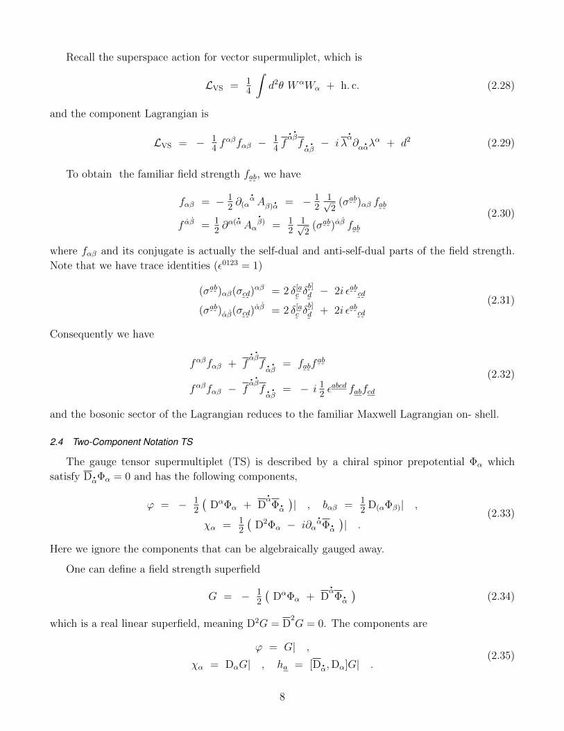
1 Introduction
Previously [1], we have studied the question of constructing 1D, N = 4 extensions of SYK
models [2–4] by using a technique of starting with 4D, N = 1 supermultiplets and compactifying
them to 1D, N = 4 supermultiplets. In 4D superspace, the chiral [5–9], vector [10, 11], and
tensor [12] supermultiplets are all valid candidates to take as starting points. The reason for this
is the fact, that under such a reduction, the notion of spin vanishes and one is simply left with a
number of distinct 1D, N = 4 supermultiplets. However, these are not the complete “roll call of
the 1D, N = 4 supermultiplet zoo.” There is one more member, the 4D, N = 1 complex linear
supermultiplet and it can be used as a starting point. So a more complete analysis requires including
this final supermultiplet and assessing its utility in the attempt to construct the most general 1D,
N = 4 supersymmetrical extension of SYK-type models.
To accomplish this goal, it will be necessary to reexamine a little recognized property first
enunciated in a paper [13] with the title, “Linear and chiral superfields are usefully inequivalent.”
This property asserts that a given on-shell spectrum of free component fields can have multiple
embeddings within distinct superfields such that the most general supersymmetric interactions of
these fields requires use of the multiple embeddings. The use of this principle, to our knowledge,
first appeared in a 1984 publication [14] that uncovered “twisted chiral superfields” and “twisted
superpotentials” before their use in the important discovery of mirror symmetry.
The title of the paper by Hubsch [13] exactly describes the gateway for our investigation of 4D,
N = 1 actions that possess the required higher n-point functions of fermions in the context where
the spin spectrum of fields does not exceed one-half. Examples of such non-supersymmetrical
Lagrangians [15–18], either regarded as effective actions or descriptions of fundamental physics,
have a storied history in the field. Perhaps the Fermi Universal Theory of the Weak Interactions
is the greatest in this approach as it pointed the direction to the triumphal construction of the
renormalizable QFT needed for the flavor interactions of the Standard Model.
In addition to chiral, vector and tensor supermultiplets, in this paper we also utilize the complex
linear supermultiplet, whose existence was introduced in the literature via a study [19] of superfield
supergravity. Thereafter, [20–22] a literature began to evolve regarding this supermultiplet. Like
the chiral supermultiplet, its propagating degrees of freedom consist only of fields with spins of
one-half and zero. However, unlike the real linear supermultiplet, there are no gauge fields in its
spectrum. Thus, it is not a cavil against the chiral supermultiplet to note that if one is interested
in a 4D, N = 1 supersymmetrical theory that possesses:
(a.) no gauge fields in it spectrum,
(b.) SYK type 2n-point couplings among fermions, and
(c.) no higher derivative for the fermions,
requires the use of the chiral supermultiplet together with the complex linear supermultiplet.
For the convenience of the reader, references [19–35] are provided in the bibliography of this
work as a guide to the literature surrounding the development and study of the complex linear
supermultiplet. A bottom line demonstration accomplished in this work is a proof of how essential
and critical the useful inequivalence is to the construction of SYK type models with degrees of
SUSY extension greater than two. Our successful construction of models with N = 4 SUSY most
4
Page 5
certainly raises possibility that there may exist an ultimate such model at some maximal even larger
value of N with unusual properties.
In the realm of phenomenological models that incorporate SUSY, it is essentially a universal
truth that these are built upon the chiral supermultiplet. With complex linear supermultiplet being
all but ignored. This implies there is an entire realm in the model space of such constructions that
has never been explored.
We organize our paper in the following manner. In section 2, we review the two-component
conventions for discussing the chiral supermultiplet (CS), complex linear supermultiplet (CLS),
vector supermultiplet (VS), and tensor supermultiplet (TS). Section 3 introduces the chiral currents
associated with VS and TS respectively. By modifying CLS free theory, we can obtain 4-point SYK-
type terms on-shell. Following the same idea as we discussed in [1], 3-point and q-point superfield
interactions will be introduced in section 4 and 5 respectively. 4-point SYK-type vertices emerge in
both cases when we go on-shell. Section 6 is devoted to the introduction of higher q-point superfield
interactions which gives 2(q−1)-point fermionic interactions on-shell. Section 7 shows the results for
one dimensional Lagrangians that follow from the compactification of the Lagrangians constructed
in four dimensions. The emergence of N = 4 extended supersymmetry is made manifest. In section
8 we explore the question, “Do 1D, N = 4 SYK models necessarily require propagating bosons?” By
studying two possibilities with CLS chiral current and Fayet-Iliopoulos mechanism, and the failure
of these two models shows strong evidence that one cannot construct a 1D, N = 4 SYK model
without dynamical bosons. Finally, section 9 gives conclusions. We follow the presentation of our
work with an appendix and a bibliography.
2 Review of 4D,N = 1 Theories in Two-Component Notation
The derivations below use the same convention as the book Superspace. We list the convention
as well as some useful identities in Appendix A.
2.1 Two-Component Notation CS
Recall the superspace action for chiral supermultiplet (CS), which is
LCS =
∫d2θd2θ ΦΦ =
1
4DαDαD
.αD.α (ΦΦ)| , (2.1)
and the component fields are defined as
A = Φ| , ψα = DαΦ| , F = D2Φ| , (2.2)
with propagating complex scalar bosonic A and spinor fields ψα. One can then derive the D-
equations that follow from these definitions.
DαA = ψα , DαA = 0 , (2.3)
Dα ψβ = − Cαβ F , Dα ψβ = i ∂βαA , (2.4)
Dα F = 0 , Dα F = i ∂αα ψα . (2.5)
The Lagrangian in terms of component fields takes the form
LCS = (A)A − i ψα ∂α.αψ.α + FF . (2.6)
5
Page 6
2.2 Two-Component Notation CLS
A complex linear supermultiplet (CLS) can be described by a complex linear superfield Σ which
satisfy the constraint
D2Σ = 0 . (2.7)
Its component fields are defined as
B = Σ| ,
ρα = DαΣ| , ζ.α = D.αΣ| ,
H = D2Σ| , Uα.α = D.αDαΣ| , Uα.α = − DαD.αΣ| ,
β.α =1
2DαD.αDαΣ| ,
(2.8)
with propagating complex scalar bosonic B and and spinor fields ζα. One can then derive the
D-equations that follow from these definitions.
DαB = ρα , DαB = ζ α , (2.9)
Dα ρβ = − CαβH , Dα ρβ = Uβα , (2.10)
Dα ζ β = i ∂αβ B − Uαβ , Dα ζ β = 0 , (2.11)
DαH = 0 , DαH = i2 ∂
αα ρα − βα , (2.12)
Dα Uββ = i∂αβ ρβ + i2 Cαβ∂
γβργ − Cαβββ , Dα Uββ = iCαβ∂β
γζ γ , (2.13)
Dα ββ = − i2 ∂αβH , Dα ββ = i
2∂αβ Uαα + ∂αα∂αβB + i ∂ααUαβ . (2.14)
Recall the superspace action for complex linear supermuliplet, which is
LCLS = −∫d2θd2θ ΣΣ = − 1
4DαDαD
.αD.α ΣΣ | (2.15)
and this implies a component Lagrangian
LCLS = (B)B − HH + Uα.αUα.α − i ζα ∂
α.αζ.α + βαρα + β
.αρ.α (2.16)
One can modify the CLS constraint [22] by introducing one more copy of the chiral superfield
in the form of Q(Φ),
D2Σ = Q(Φ) , D2Σ = Q(Φ) . (2.17)
where Q(Φ) is an arbitrary function of Φ. Direct calculations in the presence of this modification
tell us
D2D2Σ = Σ + [
1
2Q′′(D
.αΦ)(D.αΦ) + Q′(D2
Φ) ] + i ∂α.αD.αDαΣ ,
D2D2Σ =
1
2Q′′(DαΦ)(DαΦ) + Q′(D2Φ) ,
(2.18)
then the Lagrangian in terms of component fields is
LCLS,Q = (B)B − HH + Uα.αUα.α − i ζα ∂
α.αζ.α + βαρα + β
.αρ.α
− QQ +− Q′BF − Q′ζαψα − 1
2 Q′′Bψαψα + h. c.
(2.19)
6
Page 7
By introducing the Q(Φ) field, we connect CLS with CS and we can move one step further to
discuss their simplest dynamical relations. Let’s consider LCS + LCLS and focus on the bosonic
sector only,
LB = (A)A + FF + (B)B − HH + Uα.αUα.α
− BQ′F − BQ′F − QQ(2.20)
Consider the on-shell Lagrangian by eliminating the auxiliary fields F , H, and Uα.α.
Lon−shellB = (A)A + (B)B − QQ − BBQ′Q′ (2.21)
If we takeQ = −mΦ withm a positive parameter, the on-shell Lagrangian contains−m2(AA+BB),
indicating that these two fields have the same mass. If we turn to the fermionic sector of (2.3) and
(2.19) using Q = −mΦ, then it is seen that the two-component fermions ζα and ψ.α together form
a massive Dirac fermion with the same mass as the bosons.
2.3 Two-Component Notation VS
The quantity V is an unconstrained real scalar superfield satisfying V = V which defines com-
ponent fields viaAα.α = 1
2 [D.α,Dα]V | ,
λα = iD2DαV | , λ.α = − iD2D.αV | ,
d = 12 DαD
2DαV | ,
(2.22)
which describes the vector supermultiplet (VS). These are the only components which cannot be
gauged away by non-derivative gauge transformations. In Wess-Zumino gauge, we retain these
components only.
One can define the gauge invariant superfield, Wα, field strength via
Wα = iD2DαV , W .α = − iD2D.αV , (2.23)
and one sees that it is chiral (D.αWα = 0). The components are
λα = Wα| ,
fαβ = 12 D(αWβ)| , f.
α.β
= − 12 D(.αW .β)
| , d = − i12 DαWα| = i12 D.αW .α| ,
i∂α.αλ.α = D2Wα| .
(2.24)
One can then derive the D-equations that follow from these definitions.
Dα λβ = fαβ − iCαβ d , Dα λβ = 0 , (2.25)
Dα fβγ = − i2 Cα(β∂γ)
α λα , Dα fβγ = i2 ∂(β|α λ|γ) , (2.26)
Dα d = − 12 ∂α
α λα , Dα d = 12 ∂
βα λβ . (2.27)
7
Page 8
Recall the superspace action for vector supermuliplet, which is
LVS = 14
∫d2θ WαWα + h. c. (2.28)
and the component Lagrangian is
LVS = − 14 f
αβfαβ − 14 f.α.βf.α.β− i λ
.α∂α.αλα + d2 (2.29)
To obtain the familiar field strength f˜a˜b, we have
fαβ = − 12 ∂(α
.αAβ)
.α = − 1
21√2
(σ˜a˜b)αβ f
˜a˜b
f αβ = 12 ∂
α(.αAα
.β) = 1
21√2
(σ˜a˜b)αβ f
˜a˜b
(2.30)
where fαβ and its conjugate is actually the self-dual and anti-self-dual parts of the field strength.
Note that we have trace identities (ε0123 = 1)
(σ˜a˜b)αβ(σ
˜c˜d)αβ = 2 δ[
˜a
˜c δ˜
b]
˜d − 2i ε˜
a˜b
˜c˜d
(σ˜a˜b)αβ(σ
˜c˜d)αβ = 2 δ[
˜a
˜c δ˜
b]
˜d + 2i ε˜
a˜b
˜c˜d
(2.31)
Consequently we have
fαβfαβ + f.α.βf.α.β
= f˜a˜bf˜
a˜b
fαβfαβ − f.α.βf.α.β
= − i 12 ε
abcd fabfcd
(2.32)
and the bosonic sector of the Lagrangian reduces to the familiar Maxwell Lagrangian on- shell.
2.4 Two-Component Notation TS
The gauge tensor supermultiplet (TS) is described by a chiral spinor prepotential Φα which
satisfy D.αΦα = 0 and has the following components,
ϕ = − 12
(DαΦα + D
.αΦ.α)| , bαβ = 1
2 D(αΦβ)| ,
χα = 12
(D2Φα − i∂α
.αΦ.α
)| .
(2.33)
Here we ignore the components that can be algebraically gauged away.
One can define a field strength superfield
G = − 12
(DαΦα + D
.αΦ.α)
(2.34)
which is a real linear superfield, meaning D2G = D2G = 0. The components are
ϕ = G| ,
χα = DαG| , ha = [D.α,Dα]G| .(2.35)
8
Page 9
Here ha is a component field strength given by
ha = i(∂β.αbαβ − ∂α
.βb.α.β
). (2.36)
One can then derive the D-equations that follow from these definitions.
Dα ϕ = χα , Dα ϕ = χα , (2.37)
Dα χβ = 0 , Dα χβ = i2 ∂βα ϕ+ 1
2 hβα , (2.38)
Dα hββ = i ∂αβ χβ − i Cαβ ∂γβχγ , Dα hββ = iCαβ ∂β
γχγ − i ∂βα χβ . (2.39)
The superspace Lagrangian is
LTS = − 12
∫d2θd2θ G2 , (2.40)
and the corresponding component Lagrangian is
LTS = 14 ϕϕ + 1
4 haha − i χ
.α∂α.αχα . (2.41)
9
Page 10
3 From Modified CLS Free Theory to 4-Point On-Shell SYK
We can construct chiral currents [1]
JVS = WαWα , (3.1)
JTS = (D.αG)(D.αG) . (3.2)
They all satisfy the chiral condition
D.αJ = 0 . (3.3)
We can also define the cojugate (anti-chiral) currents
J VS = W.αW .α , (3.4)
J TS = (DαG)(DαG) . (3.5)
where (J )∗ = J and imply the equation D.αJ = 0.
Recalling (2.17)
D2Σ = Q(Φ) , D2Σ = Q(Φ) , (3.6)
One could modify the arguments of these Q functions
QA(Φ) −→ QA(J ) (3.7)
with the form
QA(J ) = κABCJBC (3.8)
so that
QQ ∼ κκ∗JJ ∼ κκ∗ψψψψ (3.9)
and we obtain the 4-pt SYK-type terms!
Note that one can also define chiral currents from the CLS by constructing such currents from
products of (D.αΣB), i.e.
J B1B2CLS = (D.αΣB1)(D.αΣB2) , (3.10)
which satisfies the chiral condition
D.β J B1B2CLS = 0 , (3.11)
when we choose Q = 0 is the simplest such example. Therefore we will not use this current in the
remainder of this chapter, as we will discuss the application of it in the next chapter.
3.1 CLS,Q(VS)
LCLS,Q(VS) = −∫d2θd2θ Σ
AΣA = − 1
4DαDαD
.αD.α Σ
AΣA | (3.12)
with
D2ΣA = κABCJ
BCVS , D2ΣA = κ∗ABCJ
BCVS (3.13)
10
Page 11
The Lagrangian in terms of component fields is
LVS+CLS,Q(VS) = − 14 f
αβ Afαβ A −14 f.α.β Af.α.β A− i λ
.α A∂α.αλαA + dAdA
+ (BA
)BA − HAHA + UAα.α
UAα.α − i ζAα ∂α.αζA.α + βAαρAα + β
A.αρA.α
− κE AB κ∗ECD λ
Aα λBα λC.βλD.β
+κABC
[i2B
AλαB∂α.αλ
.αC
+ BAfαβ Bf Cαβ − 2B
AdBdC
+ 2ζαAf BαβλβC + i2ζαAdBλCα
]+ h. c.
(3.14)
Although the off-shell Lagrangian already gives us the four-fermion SYK type term, the on-
shell Lagrangian is still interesting, and it gives us more four-fermion coupling terms which involve
fermions from the different multiplets.
Lon−shellVS+CLS,Q(VS) = − κE AB κ
∗ECD λ
Aα λBα λC.βλD.β
+κAEB κC
ED ζAα λBα ζ
Cβ λDβ − κAEB κ∗CED ζAα λBα ζ
C.βλD.β
+ h. c.
+ · · ·(3.15)
3.2 CLS,Q(TS)
In this subsection, our starting point is
LCLS,Q(TS) = −∫d2θd2θ Σ
AΣA = − 1
4DαDαD
.αD.α Σ
AΣA | (3.16)
with
D2ΣA = κABCJ
BCTS , D2ΣA = κ∗ABCJ
BCTS (3.17)
The Lagrangian in terms of component fields is
LTS+CLS,Q(TS) = 14 ϕAϕA + 1
4 hAahAa − i χA
.α∂α.αχαA
+ (BA
)BA − HAHA + UAα.α
UAα.α − i ζAα ∂α.αζA.α + βAαρAα + β
A.αρA.α
− κ∗E AB κE CD χAα χBα χ
C.β χD.
β
+− κABC
[− 2B
A(i∂
β.βχBβ)χC
.β − 1
4BA(i∂α.βϕB − hB
α.β
)(i∂α.βϕC − hCα
.β)
− ζAα(i∂α.βϕB − hB
α.β
)χC.β]
+ h. c.
(3.18)
The EoMs (i.e. ’equations of motion’) for the auxiliary fields are trivial: all auxiliary fields vanish.
So if we set HA = UAα.α = βAα = ρAα = 0 to obtain the on-shell Lagrangian.
11
Page 12
4 From 3-Point Off-Shell Vertices to 4-Point On-Shell SYK
4.1 CS + CLS + 3PT-B
Now, let us introduce a 3-point interaction between a complex anti-linear superfield and two
chiral superfields. The full superfield Lagrangian is
LCS+CLS+3PT−B =
∫d2θ d2θ
[ΦA
ΦA − ΣA
ΣA
]+ ∫
d2θ d2θ[κABC Σ
AΦBΦC
]+ h. c.
,
(4.1)
and the interaction term leads to the result
L3PT−B = 14 κABC DαDαD
.αD.α
[ΣA
ΦBΦC]
+ h. c.
= 12 κABC DαDα
[ (D
2ΣA)
ΦBΦC]
+ h. c.
= κABC
− (B
A)ABAC + Q′AD(A)ABACF
D+ i (∂α
.αUAα.α)ABAC
+ 12 Q
′′ADE(A)ABACψ
D.αψE.α + i (∂α
.αρA.
α)ψBαA
C − 2 βAαψBαAC
+ 2HAFBAC + H
AψBαψCα
+ h. c.
(4.2)
The complete off-shell Lagrangian is
Loff−shellCS+CLS+3PT−B = (A
A)AA + FAFA + (B
A)BA − HAHA + U
α.α
A UAα.α
− BAQ′AB(A)FB − B
AQ′AB(A)FB − QA(A)QA(A)
− i ψAα ∂α.αψA.α − i ζAα ∂
α.αζA.α − Q′ψαζα − Q
′ABψ.α
BζA.α− 1
2Q′′ABC(A)ψαBψCαBA −
1
2Q′′ABC(A)ψ
.α
BψC.αBA + βAαρAα + βA.αρA.α
+κABC
[− (B
A)ABAC + Q′AD(A)ABACF
D − 2i UAα.α(∂α
.αAB)AC
+ 12 Q
′′ADE(A)ABACψ
D.αψE.α − i ρA.
α(∂α.αψBα)AC − i ρA.
αψBα(∂α
.αAC) − 2 βAαψBαA
C
+ 2HAFBAC + H
AψBαψCα
]+ h. c.
(4.3)
When working through the EoMs for all of the auxiliary fields, one finds there is one interesting
term whose leading contribution is a four-fermion SYK type term.
Lon−shellCS+CLS+3PT−B =
κABC κ∗GDE
δAG + YAGψBα ψCα ψ
D.αψE.α + · · ·
= κABC κ∗ADE ψ
Bα ψCα ψD.αψE.α + · · ·
(4.4)
where
YAG = 4 κABC κ∗GBD AC AD
. (4.5)
12
Page 13
4.2 CS + CLS + 3PT-A + 3PT-B
Recalling the 3PT-A interaction
L3PT−A =
∫d2θ d2θ κABC Φ
AΦBΦC + h. c.
= 14 κABC DαDα D
.βD.β
[ΦA
ΦBΦC]| + h. c.
= κABC
[(A
A)ABAC + 2 (i∂α
.αψA.α )ψBαA
C + 2FAFBAC + F
AψBαψCα
]+ h. c. ,
(4.6)
the complete off-shell Lagrangian is
Loff−shellCS+CLS++3PT−A+3PT−B = (A
A)AA + FAFA + (B
A)BA − HAHA + U
α.α
A UAα.α
− BAQ′AB(A)FB − B
AQ′AB(A)FB − QA(A)QA(A)
− i ψAα ∂α.αψA.α − i ζAα ∂
α.αζA.α − Q′ψαζα − Q
′ABψ.α
BζA.α− 1
2Q′′ABC(A)ψαBψCαBA −
1
2Q′′ABC(A)ψ
.α
BψC.αBA + βAαρAα + βA.αρA.α
+κABC
[(A
A)ABAC + 2 (i∂α
.αψA.α )ψBαA
C
+ 2FAFBAC + F
AψBαψCα
]+ h. c.
+κABC
[− (B
A)ABAC + Q′AD(A)ABACF
D − 2i UAα.α(∂α
.αAB)AC
+ 12 Q
′′ADE(A)ABACψ
D.αψE.α − i ρA.
α(∂α.αψBα)AC − i ρA.
αψBα(∂α
.αAC)
− 2 βAαψBαAC + 2H
AFBAC + H
AψBαψCα
]+ h. c.
,
(4.7)
after the complete derivation of the component results.
Deriving the equations of motion for auxiliary fields F and H yields
FA[δDA + YDA + YAD
]+ Y BDH
B = − (κψψ)D + Q′BD(B − κAA
)B(4.8)
HA = YABFB + (κψψ)A (4.9)
where the Y ’s are objects linear in A or A defined as
YDA = 2κDAC AC , YDA = 2κ∗DAC A
C,
YDA = 2 κDAC AC , Y DA = 2 κ∗DAC A
C,
(4.10)
and the expressions with suppressed indices possess the definitions as
(κψψ)A = κABC ψαBψCα ,
(κψψ)A = κABC ψαBψCα ,
(κAA)A = κABC ABAC .
(4.11)
13
Page 14
We note when expansion of the denominators, imply
1
δAB + YAB=
∞∑j=0
(−1)j(Yj)BA
= δBA − YBA + YBCYCA − YBCYCDYDA + · · · .
(4.12)
and the altitude of the indices are lifted and the first and second indices flip. This is because we
treat these as matrix multiplications and the R.H.S. consists of the inverses of both the identity
matrix δAB and the Y-matrix YAB, which are δBA and YBA respectively.
Thus, we find
Lon−shellF,H = (κψψ)A(κ∗ψψ)A
−
[(κψψ)B + Y EB (κψψ)E
] [(κ∗ψψ)A + YDA (κ∗ψψ)D
]δBA + YBA + YAB + Y
CBYCA
+ O(Q′) .(4.13)
There are two terms whose leading contributions are four-fermion SYK type terms. The LF,H sector
is the only one that can contribute to SYK type terms. Explicitly, these leading terms are
Lon−shellCS+CLS+3PT−A+3PT−B = − κABC κ
∗ADE ψ
Bα ψCα ψD.αψE.α + κABC κ
∗ADE ψ
Bα ψCα ψD.αψE.α + · · ·
(4.14)
Note that if we set κABC = κABC, all four-fermion terms vanish. We can see this by simply setting
ΩAB = δAD + YAB, then the on-shell LF,H sector becomes
Lon−shellF,H = (κψψ)A(κ∗ψψ)A −
ΩCB
ΩDA
ΩEB
ΩEA(κψψ)C(κ
∗ψψ)D + O(Q′)
= (κψψ)A(κ∗ψψ)A − ΩCB
ΩDA(Ω−1
)BE(Ω−1)AE
(κψψ)C(κ∗ψψ)D + O(Q′)
= (κψψ)A(κ∗ψψ)A − δCEδDE (κψψ)C(κ
∗ψψ)D + O(Q′) = O(Q′)
(4.15)
The vanishing of the solely four fermion terms for this choice κABC = κABC is likely a strong
indication of an extended, but hidden, N = 2 supersymmetry (in 4D, i.e. N = 8 in 1D) of the
model. We make this assertion on the basis of past results in the literature [22–34], wherein it has
been note that a pair of supermultiplets described by one chiral supermultiplet and one complex
linear supermultiplet provides exactly the spectrum of component fields required to describe a Dirac
spinor, two scalars and two psuedoscalars of a 4D, N = 2 supersymmetric hypermultiplet system.
14
Page 15
5 From q-Point Off-Shell Vertices to 4-Point On-Shell SYK
5.1 CS + CLS + nCLS-A
An n-point superfield interaction among one chiral and a polynomial of complex linear superfields
with kinetic terms can be written in the form
LCS+CLS+nCLS−A =
∫d2θ d2θ
ΦA
ΦA − ΣA
ΣA +[
ΦAPA(Σ) + h. c.]
. (5.1)
The interaction term can be expressed as
LnCLS−A = 14 DαDα D
.αD.α[
ΦAPA(Σ)]
+ h. c. . (5.2)
We let
PA(Σ) =P∑i=2
κ(i)
AB1···Bi
i∏k=1
ΣBk , (5.3)
where κ(i)
AB1···Bi’s are arbitrary coefficients, and the degree of the polynomial is P . Note that the
interaction terms start from cubic order. Obviously, B1 to Bi indices for any 1 ≤ i ≤ P on the
coefficient κ(i)
AB1···Biare symmetric. We then have
P ′′AB1B2(Σ) = 2κ(2)
AB1B2+
P∑j=3
j(j − 1)κ(j)
AB1···Bj
j∏k=3
ΣBk , (5.4)
P ′′′AB1B2B3(Σ) = 6κ(3)
AB1B2B3+
P∑j=4
j(j − 1)(j − 2)κ(j)
AB1···Bj
j∏k=4
ΣBk , (5.5)
P ′′′′AB1B2B3B4(Σ) = 24κ(4)
AB1B2B3B4+
P∑j=5
j(j − 1)(j − 2)(j − 3)κ(j)
AB1···Bj
j∏k=5
ΣBk . (5.6)
15
Page 16
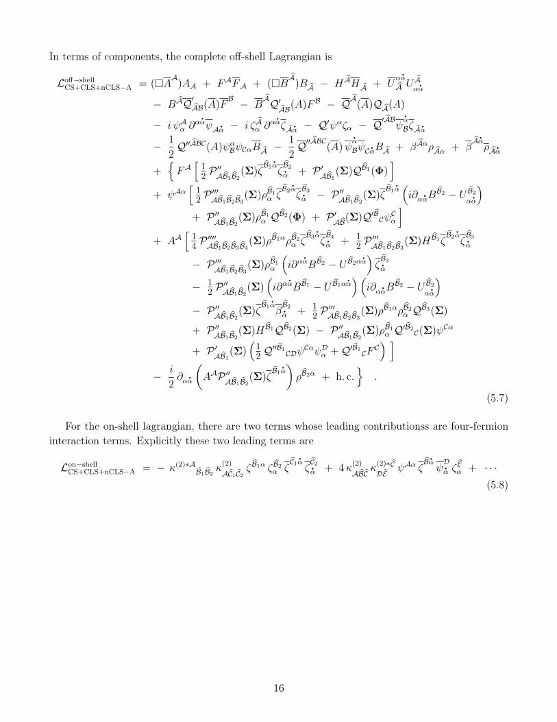
In terms of components, the complete off-shell Lagrangian is
Loff−shellCS+CLS+nCLS−A = (A
A)AA + FAFA + (B
A)BA − HAHA + U
α.α
A UAα.α
− BAQ′AB(A)FB − B
AQ′AB(A)FB − QA(A)QA(A)
− i ψAα ∂α.αψA.α − i ζAα ∂
α.αζA.α − Q′ψαζα − Q
′ABψ.α
BζA.α− 1
2Q′′ABC(A)ψαBψCαBA −
1
2Q′′ABC(A)ψ
.α
BψC.αBA + βAαρAα + βA.αρA.α
+FA[
12 P
′′AB1B2
(Σ)ζB1.αζB2.α + P ′AB1(Σ)QB1(Φ)
]+ ψAα
[12 P
′′′AB1B2B3
(Σ)ρB1α ζB2.αζB3.α − P ′′AB1B2(Σ)ζ
B1.α(i∂α.αBB2 − U B2α.α
)+ P ′′AB1B2(Σ)ρB1α QB2(Φ) + P ′AB(Σ)Q′BCψCα
]+ AA
[14 P
′′′′AB1B2B3B4
(Σ)ρB1αρB2α ζB3.αζB4.α + 1
2 P′′′AB1B2B3
(Σ)H B1ζB2.αζB3.α
− P ′′′AB1B2B3(Σ)ρB1α
(i∂α.αBB2 − U B2α
.α)ζB3.α
− 12 P
′′AB1B2
(Σ)(i∂α.αBB1 − U B1α
.α)(
i∂α.αBB2 − U B2α.α)
− P ′′AB1B2(Σ)ζB1.αβB2.α + 1
2 P′′′AB1B2B3
(Σ)ρB1αρB2α QB3(Σ)
+ P ′′AB1B2(Σ)H B1QB2(Σ) − P ′′AB1B2(Σ)ρB1α Q′B2C(Σ)ψCα
+ P ′AB1(Σ)(
12 Q
′′B1CDψ
CαψDα +Q′B1CF C) ]
− i
2∂α.α
(AAP ′′AB1B2(Σ)ζ
B1.α)ρB2α + h. c.
.
(5.7)
For the on-shell lagrangian, there are two terms whose leading contributionss are four-fermion
interaction terms. Explicitly these two leading terms are
Lon−shellCS+CLS+nCLS−A = − κ(2)∗A
B1B2 κ(2)
AC1C2ζ B1α ζ B2α ζ
C1.αζC2.α + 4κ
(2)
ABCκ
(2)∗DEC ψAα ζ
B.αψD.α ζEα + · · ·
(5.8)
16
Page 17
6 From q-Point Off-Shell Vertices to 2(q − 1)-Point On-Shell SYK
6.1 CS + CLS + nCLS-B
Now consider the standard complex linear supermultiplet, we have
D2
Σ = 0 , (6.1)
therefore
D.β[
(D.αΣ)(D.αΣ)
]= 2 (D
.βD.αΣ)(D.αΣ) = − 2 (D
2Σ)(D
.βΣ) = 0 , (6.2)
Recall the current
J B1B2CLS = (D.αΣB1)(D.αΣB2) , (6.3)
satisfies the chiral condition
D.β J B1B2CLS = 0 . (6.4)
Also defining
J B1B2CLS = (DαΣB1
)(DαΣB2
) , (6.5)
and (J )∗ = J . The full superfield Lagrangian is
LCS+CLS+nCLS−B =
∫d2θ d2θ
[ΦA
ΦA − ΣAΣA
]+ ∫
d2θ[
ΦAFA(JCLS)]
+ h. c.
,(6.6)
and the nCLS-B piece is
LnCLS−B = 12 DαDα
[ΦAFA(JCLS)
]+ h. c. , (6.7)
where
FA(JCLS) =P∑i=1
κ(i)
AB1B2···B2i−1B2i
i∏k=1
J B2k−1B2kCLS , (6.8)
FA(J CLS) =P∑i=1
κ(i)∗AB1B2···B2i−1B2i
i∏k=1
J B2k−1B2kCLS . (6.9)
We obtain the off-shell component description as follows.
Loff−shellCS+CLS+nCLS−B = (A
A)AA + FAFA + (B
A)BA − HAHA + U
α.α
A UAα.α
− i ψAα ∂α.αψA.α − i ζAα ∂
α.αζA.α + βAαρAα + β
A.αρA.α
+FAFA(JCLS) − 2ψAαF ′AB1B2(JCLS)ζ
B1.α(i∂α.αBB2 − U B2α.α
)+ AA
[2F ′′AB1B2B3B4(JCLS)ζ
B1.α(i∂α.αBB2 − U B2α.α
)ζB3.β
(i∂α.βBB4 − U B4α
.β)
− 12 F
′AB1B2
(JCLS)(i∂α.αBB1 − U B1α
.α)(
i∂α.αBB2 − U B2α.α)
− F ′AB1B2(JCLS)ζB1.αβB2.α
]− i
2∂α.α
(AAF ′AB1B2(JCLS)ζ
B1.α)ρB2α + h. c.
.
(6.10)
17
Page 18
The LF sector of the on-shell Lagrangian clearly describes the 2q-fermion SYK type interactions
Lon−shellF = −
P∑i,j=1
κ(i)AB1···B2iκ
(j)∗AC1···C2j
i∏k=1
j∏l=1
ζB2k−1
.αζB2k.α ζ C2l−1αζ C2lα . (6.11)
Moreover, there is also a term comeing from the LU sector of the on-shell lagrangian which is also
purely fermionic.
Lon−shellU = 4
P∑i,j=1
κ(i)ABEF3···F2i
κ(j)∗CDEG3···G2j
i∏k=2
j∏l=2
ζF2k−1
.βζF2k.βζ G2l−1βζ G2lβ ψAαζ
B.αψD.α ζEα . (6.12)
18
Page 19
7 1D,N = 4 SYK Models
Given that in 4D,
∂αα = (σ˜b)αα ∂
˜b , ∂
˜b =
1
2(σ
˜b)αα ∂αα (7.1)
where the˜b = (τ, x, y, z) labelling the 4D spacetime Cartesian coordinate and (σ˜
b)αα is the standard
Pauli matrix representation with the zeroth component as the identity matrix, so numerically we
have
(σ˜0)αα =
(1 0
0 1
):= δαα , (σ˜
0)αα =
(−1 0
0 −1
):= − δαα . (7.2)
where the metric is defined as
η˜a˜b = η˜
a˜b = diag(−1, 1, 1, 1) , (7.3)
and the spinor metric is defined as
Cαβ = Cαβ =
(0 −ii 0
), Cαβ = C αβ =
(0 i
−i 0
). (7.4)
One can obtain the following identities
(σ˜b)αα (σ˜
c)αα = 2 δ˜b˜c , (σ˜
b)αα (σ˜b)ββ = 2 δα
β δαβ . (7.5)
When we carry out the dimension reduction, we have
∂˜a →
∂0 = ∂τ
∂i = 0, ∂αα → δαα ∂τ , ∂αα → − δαα ∂τ , (7.6)
and
= ∂˜b∂
˜b =
1
2∂αα ∂αα → − ∂τ∂τ := − ∂2
τ . (7.7)
These rules suffice to obtain explicit results for component level expressions. In our subsequent
presentations, we utilize the equations above.
7.1 CLS,Q(VS)
In the case of the CLS. Q(VS) Lagrangian we find in 1D
LVS+CLS,Q(VS) = − 14 f
αβ Afαβ A −14 f.α.β Af.α.β A
+ i λ.α Aδαα ∂τλ
αA + dAdA
+ (∂τBA
)(∂τBA) − HAHA + UAα.α
UAα.α − i ζAα δαα ∂τζA.α
+ βAαρAα + βA.αρA.α − κE AB κ
∗ECD λ
Aα λBα λC.βλD.β
+κABC
[− i2B
AλαBδαα ∂τλ
.αC
+ BAfαβ Bf Cαβ − 2B
AdBdC
+ 2ζαAf BαβλβC + i2ζαAdBλCα
]+ h. c.
.
(7.8)
19
Page 20
7.2 CLS,Q(TS)
In the case of the CLS. Q(TS) Lagrangian we find in 1D
LTS+CLS,Q(TS) = 14 (∂τϕ
A) (∂τϕA) + 14 hAahAa + i χA
.αδα.α∂τχαA
+ (∂τBA
)(∂τBA) − HAHA + UAα.α
UAα.α − i ζAα δα.α∂τζA.α
+ βAαρAα + βA.αρA.α − κ∗E AB κE CD χ
Aα χBα χC.β χD.
β
+− κABC
[2i B
Aδβ.β(∂τχ
Bβ)χC.β
+ 14BA(iδα.β∂τϕ
B + hBα.β
)(iδα.β∂τϕ
C − hCα.β)
+ ζAα(iδα.β∂τϕ
B + hBα.β
)χC.β]
+ h. c.
.
(7.9)
7.3 CS + CLS + 3PT-B
In the case of the CS + CLS + 3PT-B Lagrangian we find in 1D
Loff−shellCS+CLS+3PT−B = (∂τA
A)(∂τAA) + FAFA + (∂τB
A)(∂τBA) − HAHA + U
α.α
A UAα.α
− BAQ′AB(A)FB − B
AQ′AB(A)FB − QA(A)QA(A)
− i ψAα δα.α∂τψA.α − i ζAα δ
α.α∂τζA.α − Q′ψαζα − Q
′ABψ.α
BζA.α− 1
2Q′′ABC(A)ψαBψCαBA −
1
2Q′′ABC(A)ψ
.α
BψC.αBA + βAαρAα + βA.αρA.α
+κABC
[− 2 (∂τB
A)(∂τA
B)AC + Q′AD(A)ABACFD − 2i δα
.αUAα.α(∂τA
B)AC
+ 12 Q
′′ADE(A)ABACψ
D.αψE.α − i ρA.
αδα.α(∂τψ
Bα)AC − i ρA.
αψBαδ
α.α(∂τA
C)
− 2 βAαψBαAC + 2H
AFBAC + H
AψBαψCα
]+ h. c.
.
(7.10)
20
Page 21
7.4 CS + CLS + 3PT-A + 3PT-B
In the case of the CS + CLS + 3PT-A + 3PT-B Lagrangian, its 1D form is
Loff−shellCS+CLS++3PT−A+3PT−B = (∂τA
A)(∂τAA) + FAFA + (∂τB
A)(∂τBA) − HAHA + U
α.α
A UAα.α
− BAQ′AB(A)FB − B
AQ′AB(A)FB − QA(A)QA(A)
− i ψAα δα.α ∂τψA.α − i ζAα δ
α.α ∂τζA.α − Q′ψαζα − Q
′ABψ.α
BζA.α− 1
2Q′′ABC(A)ψαBψCαBA −
1
2Q′′ABC(A)ψ
.α
BψC.αBA+ βAαρAα + β
A.αρA.α
+κABC
[2 (∂τA
A)(∂τA
B)AC + 2 (iδα.α ∂τψ
A.α )ψBαA
C
+ 2FAFBAC + F
AψBαψCα
]+ h. c.
+κABC
[− 2 (∂τB
A)(∂τA
B)AC + Q′AD(A)ABACFD
− 2i UAα.α(δα
.α ∂τA
B)AC + 12 Q
′′ADE(A)ABACψ
D.αψE.α
− i ρA.α
(δα.α ∂τψ
Bα)AC − i ρA.
αψBα(δα
.α ∂τA
C)
− 2 βAαψBαAC + 2H
AFBAC + H
AψBαψCα
]+ h. c.
.
(7.11)
21
Page 22
7.5 CS + CLS + nCLS-A
In the case of the CS + CLS + nCLS-A Lagrangian, its 1D form is
Loff−shellCS+CLS+nCLS−A = (∂τA
A)(∂τAA) + FAFA + (∂τB
A)(∂τBA) − HAHA + U
α.α
A UAα.α
− BAQ′AB(A)FB − B
AQ′AB(A)FB − QA(A)QA(A)
− i ψAα δα.α ∂τψA.α − i ζAα δ
α.α ∂τζA.α − Q′ψαζα − Q
′ABψ.α
BζA.α− 1
2Q′′ABC(A)ψαBψCαBA −
1
2Q′′ABC(A)ψ
.α
BψC.αBA + βAαρAα + βA.αρA.α
+FA[
12 P
′′AB1B2
(Σ)ζB1.αζB2.α + P ′AB1(Σ)QB1(Φ)
]+ ψAα
[12 P
′′′AB1B2B3
(Σ)ρB1α ζB2.αζB3.α + P ′′AB1B2(Σ)ζ
B1.α(i δα.α ∂τBB2 + U B2
α.α
)+ P ′′AB1B2(Σ)ρB1α QB2(Φ) + P ′AB(Σ)Q′BCψCα
]+ AA
[14 P
′′′′AB1B2B3B4
(Σ)ρB1αρB2α ζB3.αζB4.α + 1
2 P′′′AB1B2B3
(Σ)H B1ζB2.αζB3.α
− P ′′′AB1B2B3(Σ)ρB1α
(iδα.α ∂τB
B2 − U B2α.α)ζB3.α
+ 12 P
′′AB1B2
(Σ)(iδα.α ∂τB
B1 − U B1α.α)(
iδα.α ∂τBB2 + U B2α.α
)− P ′′AB1B2(Σ)ζ
B1.αβB2.α + 1
2 P′′′AB1B2B3
(Σ)ρB1αρB2α QB3(Σ)
+ P ′′AB1B2(Σ)H B1QB2(Σ) − P ′′AB1B2(Σ)ρB1α Q′B2C(Σ)ψCα
+ P ′AB1(Σ)(
12 Q
′′B1CDψ
CαψDα +Q′B1CF C) ]
+i
2δα.α ∂τ
(AAP ′′AB1B2(Σ)ζ
B1.α)ρB2α + h. c.
.
(7.12)
7.6 CS + CLS + nCLS-B
In the case of the CS + nCLS-B Lagrangian, its 1D form is
Loff−shellCS+CLS+nCLS−B = (∂τA
A)(∂τAA) + FAFA + (∂τB
A)(∂τBA) − HAHA + U
α.α
A UAα.α
− i ψAα δα.α ∂τψA.α − i ζAα δ
α.α ∂τζA.α + βAαρAα + β
A.αρA.α
+FAFA(JCLS) + 2ψAαF ′AB1B2(JCLS)ζ
B1.α(i δα.α ∂τBB2 + U B2
α.α
)+ AA
[2F ′′AB1B2B3B4(JCLS)ζ
B1.α(δα.α ∂τBB2 − iU B2α.α
)ζB3.β
(δα.β∂τB
B4 + U B4α.β)
+ 12 F
′AB1B2
(JCLS)(iδα.α∂τB
B1 − U B1α.α)(
iδα.α∂τBB2 + U B2α.α
)− F ′AB1B2(JCLS)ζ
B1.αβB2.α
]+
i
2δα.α∂τ
(AAF ′AB1B2(JCLS)ζ
B1.α)ρB2α + h. c.
.
(7.13)
All the actionS of this section possess explicit 1D, N = 4 off-shell SUSY and SYK-type terms.
22
Page 23
8 Evidence for the Incompatibility of SYK Terms and the Absence of Dynamical Bosons
One of the questions that occur when considering 1D, N = 4 extensions of SYK models is, “Do
such model necessarily required propagating bosons?” In the confines of the work completed in [1],
there were no concrete proofs related to this matter. However, the exploration of the diversity
of models was undertaken with this question in mind. The results shown in that work covers all
reasonable possibilities known to the authors in the attempt to construct such models from the
starting point of 4D, N = 1 supermultiplets. The results were negative in every studied case.
In unpublished work, we have also explored this question by starting with 2D, (4,0) heterotic
supermultiplets [36, 37]. It is important to recognize that the smaller the number of bosonic coor-
dinates in a supermultiplet, the less restrictions result in the possible forms of the supersymmetry
transformation laws. Nonetheless, even in these theories, all N = 4 extensions of SYK models led
to the presence of propagating bosons. In the remainder of this chapter, we will explore the same
question.
8.1 An attempt with CLS chiral current
In this section, our starting point will include the possibility of using the complex linear super-
multiplet as this has been the main topic of this exploration.
Now, let us introduce an interaction between a complex anti-linear superfield and the CLS chiral
current JCLS. This means that we have Q = 0. The full superfield Lagrangian is
LCLS+3PT−C =
∫d2θ d2θ
[− Σ
AΣA
]+ ∫
d2θ d2θ[κABC Σ
A J BCCLS
]+ h. c.
=
∫d2θ d2θ
[− Σ
AΣA
]+ ∫
d2θ d2θ[κABC Σ
A(D.αΣB) (D.αΣC)
]+ h. c.
.
(8.1)
The complete off-shell Lagrangian is
Loff−shellCLS+3PT−C = − 1
2 (∂γγBA
)(∂γγBA) − HAHA + Uα.α
A UAα.α− i ζAα ∂
α.αζA.α + βAαρAα + β
A.αρA.α
+κABC
[( ∂γαB
A) (∂γγζ
B.β)ζC.β
+ i(∂α.αUAα.α)ζB.βζC.β
− 2(i2∂
α.αρA.
α− βAα
)ζB.β(i∂α.βBC − U C
α.β
)− H
A(i∂α.αBB − U Bα
.α)(
i∂α.αBC − U Cα.α)
+ 2HAζB.α( i
2∂α.αρCα − βC.α
) ]+ h. c.
.
(8.2)
One sees that the all the terms involving the dynamical boson B exist in the form of ∂B, and
therefore one can do the replace ∂B → b (b regarded as a new field) in 1D and think of it as an
auxiliary field. That means we get rid of dynamical bosons in this model.
Now let us figure out if there exists a SYK term in this model. The Equations of Motions
23
Page 24
(EoMs) are:
HA = − κABC
(i∂α.αBB − U Bα
.α)(
i∂α.αBC − U Cα.α)
+ 2κABC ζB.α( i
2∂α.αρCα − βC.α
),
(8.3)
Uα.αC = 2i κCBD ζ
B.β(∂α.αζ
D.β
) + 2i κ∗ABCHA(∂α
.αBB)
+ 2κ∗ABC
(i2∂
β.αρAβ − β
A.α)ζ Bα + 2κ∗ABCH
AUBα.α
,(8.4)
β.α
C = i κCBD ∂α.α[ζB.β(i∂α.βBD − U D
α.β
)] + i κ∗ABC∂
α.α[HAζ Bα ] , (8.5)
ρCα = 2κCBD ζB.α (−i ∂α.αBC + U C
α.α
)+ 2κ∗ABC H
Aζ Bα . (8.6)
A further calculation shows that(i2∂α.αρCα − βC.α
)= 2i κ∗AB
C ∂α.α(HAζ Bα
), (8.7)(
i2∂
β.αρAβ − β
A.α)= − 2i κABC ∂
α.α
[ζB.β(i∂α.βBC − U C
α.β
)]. (8.8)
Therefore we have a system of equations in H and U :
HD = − i 4κDBC κABE[∂α.α(HAζ Eα
) ]ζC.α
− κDBC(U Bα.α− i∂α.αBB
) (Uα.α C − i∂α
.αBC
),
(8.9)
Uα.α
D − 2κADCHAUα.α C = − i 2κ∗DBCζ
β B (∂α.αζ Cβ)+ i 4κADC κ
∗ ABE ∂
α.β[ (UBβ.β
+ i∂β.βBB)ζβ E
]ζ.α C
− i 2κADC HA (∂α.αBC
),
(8.10)
where we have ∂H in EoM of H, and ∂U in EoM of U , and they also couple. Thus the equations of
motion become differential equations, and inverting these equations would definitely put derivatives
on the fermion ζ, which means it is not possible to obtain SYK terms from this model.
24
Page 25
8.2 An attempt to utilize the Fayet-Iliopoulos mechanism
Another attempt would involve the Fayet-Iliopoulos mechanism. The Fayet-Iliopoulos term here
is a linear term in the “spectator” chiral superfield. When one does the chiral superspace integral,
one would obtain a linear auxiliary field term. Therefore, if one sticks the auxiliary field to any term
we want (e.g. a quartic fermionic SYK term here) in the off-shell Lagrangian, one would obtain
the desired term in the on-shell Lagrangian as the equation of motion of that auxiliary field would
contain a constant and the SYK term. For example, one could have
LFI−1 =
∫d2θd2θ
[ΦΦ +
(14 W
αAWαA + h. c.) ]
+ ∫
d2θ cΦ + h. c.
+ ∫
d2θ[κABCD ΦWαAW B
αWβCW D
β
]+ h. c.
,
(8.11)
since the VS field strength Wα is chiral. Note that the “spectator” chiral superfield Φ does not have
a number of copies index. So this action would lead to an off-shell Lagrangian with
Loff−shellFI−1 = FF +
cF + h. c.
+κABCD F λ
αAλBαλβCλDβ + h. c.
+ · · · , (8.12)
and the equation of motion for F would be
F + c + λαAλBαλβCλDβ = 0 . (8.13)
Therefore, the kinetic and FI terms would generate our desired on-shell term
Lon−shellFI−1 ∼ c κ λλλλ + h. c. + · · · . (8.14)
However, the problem of this action is that it would generate terms with dynamical bosons,
LFI−1 = κABCD Φ D2[WαAW B
αWβCW D
β
]+ h. c. + · · · , (8.15)
which is what we want to get rid of. Note that this action actually resembles the nVS-B model
in [1].
Now, we note that Wα is chiral, and therefore modifying this interaction term by changing Φ to
Φ (which allows us to integrate the entire superspace) would put derivatives only on Φ. This would
allow us to change all Φ’s to D2Φ and get rid of all dynamical bosons.
LFI−2 =
∫d2θd2θ
[ΦΦ +
(14 W
αAWαA + h. c.) ]
+ ∫
d2θ cΦ + h. c.
+ ∫
d2θd2θ[κABCD ΦWαAW B
αWβCW D
β
]+ h. c.
.
(8.16)
However, the linear term cannot be changed accordingly as it is chiral and cannot be integrated
over the entire superspace. Therefore we lose the ’magic power’ of the Fayet-Iliopoulos mechanism
- that is to utilize the constant c in the equation of motion of the auxiliary field to obtain any term
25
Page 26
we desire. Nonetheless, we can still try to find its off-shell component Lagrangian and take a look
at the equations of motion to see if we have any luck. The complete off-shell Langrangian is
Loff−shellFI−2 = − 1
4 fA
˜a˜bf˜
a˜b
A − i λα
A ∂αα λAα + dA dA −
12 (∂ααA)(∂ααA)− i ψα ∂αα ψα + FF
+ cF + cF +
4 κABCD F[i (∂αα λ
Aα )λBα λ
Cβ λDβ −12 fAαβ f
Bαβ λCγ λDγ
+ dA dB λCα λDα + f Aαβ λBβ f Cαγ λDγ
− 2i f Aαβ λBβ dC λDα − dA λBα dC λDα
]− 2 κABCD (∂γγ A) (∂γγ λAα)λBα λ
Cβ λDβ
− 4i κABCD (∂γγ ψγ)[f Aγα λ
Bα + i dA λBγ
]λCβ λDβ + h. c.
.
(8.17)
Notice that after using the EoMs for the auxiliary field F
F = − c− 4 κABCD
[i (∂αα λ
Aα )λBα λ
Cβ λDβ + dA dB λCα λDα − dA λBα dC λDα]
+O(fαβ) , (8.18)
and its conjugate, there are only three terms contributed by d, F , and F fields in the Lagrangian
LFI−2 ∼ dA dA − FF +[
4 κABCD (∂γγ ψγ) dA λBγ λ
Cβ λDβ + h. c.]
. (8.19)
Only when the leading term in the solution of the EoM for d field ∼ λ or λλ, we can obtain
SYK-type terms in the final on-shell Lagrangian. However, the EoM for d takes the following form
dA = − 4 κABCD F dB λCα λDα + 4 κABCD F λ
Bα dC λDα − 2 κABCD (∂γγ ψγ)λBγ λCβ λDβ +O(fαβ)
+ h. c. ,(8.20)
where we can substitute (8.18) and its conjugate into the above equation and get a cubic order
equation for d. So we obtain a conclusion that only the equation of motion of F contains pure
λ-terms, however, it takes the form of
F = − c− i4 κABCD (∂αα λAα )λBα λ
Cβ λDβ + · · · , (8.21)
which inevitably has a derivative on λ. Therefore, neither the kinetic term nor the FI-term would
generate purely fermionic terms with no derivatives acting on any of the fermions.
We could also consider the adinkra duality trick of ∂A → b in 1D. The equation of motion of
the new auxiliary field b would be
b = − 2κ(∂λ)λλλ , (8.22)
which also takes the same form as the equation of motion of F (ignoring terms with dynamical
fields other than λ). Therefore treating ∂A as an auxiliary field would not grant us the SYK term.
This is inevitable as F and ∂A has the same engineering dimension to start with.
The conclusion of this attempt is either we utilize the FI mechanism effectively via LFI−1, which
would give us the SYK term and dynamical bosons, or we modify it to LFI−2 which would get rid
of dynamical bosons but would not give us the SYK term.
26
Page 27
9 Conclusion
In [1], we constructed several 1D, N = 4 supersymmetric SYK models based on chiral super-
multiplet, vector supermultiplet, and tensor supermultiplet. In this work, we contribute to the
discussion by including the complex linear supermultiplet.
In addition to 3-point and q-point superfield vertices, we introduced a class of models based on
the modification of the CLS kinetic terms in Section 3, which is allowed by introducing a copy of VS
or TS through relaxing the complex linear constraint. This class of models has the special feature
of containing the desired 4-point SYK terms off-shell (and they will stay when we go on-shell).
In section 4.2 we study the model with two 3-point superfield vertices, one with one anti-chiral
and two chiral superfields, and another with the anti-chiral superfield changed to complex anti-
linear superfield. When the coupling constants are chosen to be the same, the four-fermion terms
vanish. This indicates a hidden N = 2 supersymmetry in the model.
Another remark is on the incompatibility of SYK terms and the absence of dynamical bosons.
The efforts described in Section 8 indicate that 1D, N = 4 models with SYK-type interactions must
include dynamical bosons. By removing dynamical bosons, we will also remove SYK terms.
“My [algebraic] methods are really methods of working
and thinking; this is why they have crept in everywhere
anonymously.”
- Amalie Emmy Noether
Acknowledgements
The research of S. J. G., Y. Hu, and S.-N. Mak is supported in part by the endowment of the
Ford Foundation Professorship of Physics at Brown University and they gratefully acknowledge the
support of the Brown Theoretical Physics Center. Work by S.-N. Mak is partially supported by
Galkin Foundation Fellowship, and work by Y. Hu is partially supported by Physics Dissertation
Fellowship at Brown University.
27
Page 28
A Superspace Conventions
In this appendix, we review the two-component notation in 4D, N = 1 superspace. First, the
algebra that super-covariant derivatives satisfy is
Dα, Dβ = Dα, Dβ = 0 (A.1)
Dα, Dβ = i∂αβ (A.2)
where α, α = 1, 2.
D2 = 12Dα Dα (A.3)
D2
= 12D
αDα (A.4)
= 12∂
αα ∂αα (A.5)∫d2θd2θ = D2 D
2 |θ→0,θ→0 (A.6)
(Dα)∗ = −Dα (A.7)
(Dα)∗ = Dα
(A.8)
→ (D2)∗ = D2
(A.9)
where ∗ means hermitian conjugation.
Useful identities:
Dα D2 = Dα D2
= 0 (A.10)
Dα D2
= D2
Dα + i∂αα Dα (A.11)
Dα
D2 = D2 Dα
+ i∂αα Dα (A.12)
Dα Dβ = − Cαβ D2 (A.13)
Dγ D2
Dγ = Dγ
D2 Dγ = 2 D2 D2
+ i∂αα Dα Dα (A.14)
D2
D2 = D2 D2
+ + i∂αα Dα Dα (A.15)
D2 D2
= D2
D2 + + i∂αα Dα Dα (A.16)
We can relate a vector label˜a in a Cartesian coordinate basis to the αα basis by a set of
Clebsch-Gordan coefficients, the Pauli matrices:
For fields : V αα =1√2
(σ˜b)αα V ˜
b , V ˜b =
1√2
(σ˜b)αα V
αα (A.17)
For derivatives : ∂αα = (σ˜b)αα ∂
˜b , ∂
˜b =
1
2(σ
˜b)αα ∂αα (A.18)
For coordinates : xαα =1
2(σ
˜b)αα x˜
b , x˜b = (σ˜
b)αα xαα (A.19)
Pauli matrices satisfy:
(σ˜a)αα (σ˜
b)αα = 2 δ˜a˜b (A.20)
(σ˜b)αα (σ
˜b)ββ = 2 δα
β δαβ (A.21)
28
Page 29
References
[1] S. J. Gates, Y. Hu and S. N. H. Mak, “On 1D, N = 4 Supersymmetric SYK-Type Models (I),”
[arXiv:2103.11899 [hep-th]].
[2] S. Sachdev and J. Ye, “Gapless spin fluid ground state in a random, quantum Heisenberg magnet,”
Phys. Rev. Lett. 70, no. 21, 3339 (1993) doi:10.1103/PhysRevLett.70.3339 [arXiv:9212030
[cond-mat]].
[3] A. Kitaev, “Hidden Correlations in the Hawking radiation and Thermal Noise,” KITP Fundamental
Physics Prize Symposium (Nov. 10, 2014), http://oneline.kitp.ucsb.edu/online/joint98/.
[4] A. Kitaev, “A simple model of quantum holography,” KITP strings seminar and Entanglement 2015
program (Feb. 12, Apr. 7, & May 27, 2015), http://oneline.kitp.ucsb.edu/online/entangled15/.
[5] Yu. A. Gol’fand and E. P. Likhtman, ”Extension of the Algebra of Poincare Group Generators and
violation of P Invariance,” JETP Lett. 13 (1971) 323.
[6] Yu. A. Gol’fand and E. P. Likhtman, Pisma Zh.Eksp. Teor. Fiz 13 (1971) 452.
[7] J. Wess, and B. Zumino, “A Lagrangian Model Invariant Under Supergauge Transformations,”
Phys. Lett. B49 (1974) 52; idem. “Supergauge Transformations in Four-Dimensions,” Nucl. Phys.
B70 (1974) 39.
[8] J. Wess, Lectures given at the Bonn Summer School 1974.
[9] P. Fayet, “Fermi-Bose Hypersymmetry,” Nucl. Phys. B113 (1976) 135.
[10] J. Wess, and B. Zumino, Nucl. Phys. B78 (1974) 1; DOI: 10.1016/0550-3213(74)90112-6.
[11] S. Ferrara, and B. Zumino Nucl. Phys. 679 (1974) 413, DOI: 10.1016/0550-3213(74)90559-8.
[12] W. Siegel, “Gauge Spinor Superfield as a Scalar Multiplet;” Phys. Lett. B 85 (1979) 333, DOI:
10.1016/0370-2693(79)91265-6.
[13] T. Hubsch, “Linear and chiral superfields are usefully inequivalent,” Class. Quant. Grav. 16 (1999)
L51-L54, DOI: 10.1088/0264-9381/16/9/101, e-Print: hep-th/9903175.
[14] S. J. Gates, Jr., “Superspace Formulation of New Nonlinear Sigma Models,” Nucl. Phys. B 238
(1984) 349, DOI: 10.1016/0550-3213(84)90456-5.
[15] W. Thirring, Ann. Phys. 3 (N.Y.) (1958), “A Soluble relativistic field theory?,” 91, DOI:
10.1016/0003-4916(58)90015-0.
[16] Y. Nambu, and G. Jona-Lasinio, “Dynamical Model of Elementary Particles Based on an Analogy
with Superconductivity. I,” Phys. Rev. 122 (1961) 345, DOI: 10.1103/PhysRev.122.345.
29
Page 30
[17] Y. Nambu, and G. Jona-Lasinio, “Dynamical Model of Elementary Particles Based on an Analogy
with Superconductivity. II,” Phys. Rev. 124 (1961) 246, DOI: 10.1103/PhysRev.124.246.
[18] D. Gross, and A. Neveu, “Dynamical symmetry breaking in asymptotically free field theories,”
Phys. Rev. D. 10 (10) (1974) 3235, DOI: 10.1103/PhysRevD.10.3235.
[19] W. Siegel, and S. J. Gates, Jr., “Superfield Supergravity,” Nucl. Phys. B147 (1979) 77-104, DOI:
10.1016/0550-3213(79)90416-4.
[20] S. J. Gates, Jr., and W. Siegel,“Variant Superfield Representations,” Nucl. Phys. B187 (1981)
389-396, DOI: 10.1016/0550-3213(81)90281-9.
[21] S. J. Gates, Jr., M. T. Grisaru, M. Rocek, and W. Siegel. Superspace Or One Thousand and One
Lessons in Supersymmetry, Front. Phys. 58 (1983) [hep-th/0108200].
[22] B. B. Deo and S. J. Gates Jr., “Comments On Nonminimal N=1 Scalar Multiplets,” Nucl. Phys.
B254 (1985) 187.
[23] I. L. Buchbinder, and S. M. Kuzenko, Ideas and methods of supersymmetry and supergravity: Or a
walk through superspace. (Studies in High Energy Physics, Cosmology and Gravitation). CRC Press.
(1998), ISBN-13: 978-0750305068.
[24] S. M. Kuzenko, “Projective superspace as a double-punctured harmonic superspace,” Int. J. Mod.
Phys. A 14, 1737 (1999), DOI: 10.1142/S0217751X99000889, [arXiv:hep-th/9806147].
[25] S. J. Gates, Jr. and S. M. Kuzenko, “The CNM Hypermultiplet Nexus,” Nucl. Phys. B543 (1999)
122, [arXiv:hep-th/9810137].
[26] S. J. Gates, Jr., T. Hubsch, S. M. Kuzenko, “CNM Models, Holomorphic Functions and Projective
Superspace C Maps,” Nucl.Phys. B557 (1999) 443, [arXiv:hep-th/9902211];
[27] S. J. Gates, Jr. and S. M. Kuzenko, “4-D, N=2 Supersymmetric Off-Shell Sigma Models on the
Cotangent Bundles of Kahler Manifolds,” Fortsch. Phys. 48, 115 (2000), DOI:
10.1002/(SICI)1521-3978(20001)48:1/3¡115::AID-PROP115¿3.0.CO;2-F”, [arXiv:hep-th/9903013].
[28] S. J. Gates Jr., T. Hubsch, and S. M. Kuzenko, “CNM models, holomorphic functions and
projective superspace C maps Nucl. Phys. B 557 (1999) 443, DOI: 10.1016/S0550-3213(99)00370-3,
[arXiv:hep-th/9902211].
[29] S. J. Gates, Jr., S. Penati, and G. Tartaglino-Mazzucchelli, “6D Supersymmetry, Projective
Superspace & 4D N = 1 Superfields,” JHEP 0609 (2006) 006 e-Print: hep-th/0604042 [hep-th];
idem., “6D supersymmetry, projective superspace and 4D, N = 1 superfields,” JHEP 0605 (2006)
051, e-Print: hep-th/0508187 [hep-th].
[30] S. J. Gates, Jr., S. Penati, and G. Tartaglino-Mazzucchelli, “6D Supersymmetric Nonlinear
Sigma-Models in 4D, N=1 Superspace,” JHEP 09 (2006) 006, DOI:
10.1088/1126-6708/2006/09/006, arXiv:: hep-th/0604042 [hep-th]
[31] M. Arai and M. Nitta, “Hyper-Kahler sigma models on (co)tangent bundles with SO(n) isometry,”
Nucl. Phys. B 745, 208 (2006), DOI: 10.1016/j.nuclphysb.2006.03.033, [arXiv:hep-th/0602277].
30
Page 31
[32] M. Arai, S. M. Kuzenko and U. Lindstrom, “Hyperkahler sigma models on cotangent bundles of
Hermitian symmetric spaces using projective superspace,” JHEP 0702, 100 (2007), DOI:
10.1063/1.2823784, [arXiv:hep-th/0612174].
[33] M. Arai, S. M. Kuzenko and U. Lindstrom, “Polar supermultiplets, Hermitian symmetric spaces and
hyperkahler metrics,” JHEP 0712, 008 (2007), DOI: 10.1063/1.2823784, [arXiv:0709.2633 [hep-th]].
[34] S. M. Kuzenko and J. Novak, “Chiral formulation for hyperkahler sigma-models on cotangent
bundles of symmetric spaces,” JHEP 0812, 072 (2008), DOI: 10.1088/1126-6708/2008/12/072,
[arXiv:0811.0218 [hep-th]].
[35] S. M. Kuzenko, “Lectures on nonlinear sigma-models in projective superspace,” J. Phys. A A43,
443001 (2010), DOI: 10.1088/1751-8113/43/44/443001, [arXiv:1004.0880 [hep-th]].
[36] S. James Gates Jr., and Lubna Rana, “Manifest (4,0) supersymmetry, sigma models and the ADHM
instanton construction,” Phys. Lett. B345 (1995) 233, DOI: 10.1016/0370-2693(94)01653-T, [arXiv:
9411091 [hep-th]].
[37] R. Dhanawittayapol, S. James Gates Jr., Lubna Rana, “A Canticle on (4,0) Supergravity-Scalar
Multiplet Systems for a “Cognoscente” Phys. Lett. B389 (1996) 264, DOI:
0.1016/S0370-2693(96)01254-3, [arXiv: 9606108 [hep-th]].
31


![(Microsoft PowerPoint - Seminario conclusivo [modalit\340 compatibilit\340])](https://static.documents.pub/doc/80x56/568bd9ab1a28ab2034a7e986/microsoft-powerpoint-seminario-conclusivo-modalit340-compatibilit340.jpg)


![(Microsoft PowerPoint - Lesson IX [modalit\340 compatibilit\340])](https://static.documents.pub/doc/80x56/585adeed1a28ab6e32926726/microsoft-powerpoint-lesson-ix-modalit340-compatibilit340.jpg)


