Absent Levels Problem

Journal of Machine Learning Research 19 (2018) 1-30 Submitted 9/16; Revised 7/18; Published 9/18

Random Forests, Decision Trees, and Categorical Predictors:The “Absent Levels” Problem

Timothy C. Au [email protected]

Google LLC

1600 Amphitheatre Parkway

Mountain View, CA 94043, USA

Editor: Sebastian Nowozin

Abstract

One advantage of decision tree based methods like random forests is their ability to nativelyhandle categorical predictors without having to first transform them (e.g., by using featureengineering techniques). However, in this paper, we show how this capability can lead toan inherent “absent levels” problem for decision tree based methods that has never beenthoroughly discussed, and whose consequences have never been carefully explored. Thisproblem occurs whenever there is an indeterminacy over how to handle an observation thathas reached a categorical split which was determined when the observation in question’slevel was absent during training. Although these incidents may appear to be innocuous, byusing Leo Breiman and Adele Cutler’s random forests FORTRAN code and the randomForestR package (Liaw and Wiener, 2002) as motivating case studies, we examine how overlookingthe absent levels problem can systematically bias a model. Furthermore, by using three realdata examples, we illustrate how absent levels can dramatically alter a model’s performancein practice, and we empirically demonstrate how some simple heuristics can be used to helpmitigate the effects of the absent levels problem until a more robust theoretical solution isfound.

Keywords: absent levels, categorical predictors, decision trees, CART, random forests

1. Introduction

Since its introduction in Breiman (2001), random forests have enjoyed much success as oneof the most widely used decision tree based methods in machine learning. But despitetheir popularity and apparent simplicity, random forests have proven to be very difficultto analyze. Indeed, many of the basic mathematical properties of the algorithm are stillnot completely well understood, and theoretical investigations have often had to rely oneither making simplifying assumptions or considering variations of the standard frameworkin order to make the analysis more tractable—see, for example, Biau et al. (2008), Biau(2012), and Denil et al. (2014).

One advantage of decision tree based methods like random forests is their ability tonatively handle categorical predictors without having to first transform them (e.g., by usingfeature engineering techniques). However, in this paper, we show how this capability canlead to an inherent “absent levels” problem for decision tree based methods that has, to thebest of our knowledge, never been thoroughly discussed, and whose consequences have neverbeen carefully explored. This problem occurs whenever there is an indeterminacy over how

c©2018 Timothy C. Au.

License: CC-BY 4.0, see https://creativecommons.org/licenses/by/4.0/. Attribution requirements are providedat http://jmlr.org/papers/v19/16-474.html.

https://creativecommons.org/licenses/by/4.0/

http://jmlr.org/papers/v19/16-474.html

Au

to handle an observation that has reached a categorical split which was determined whenthe observation in question’s level was absent during training—an issue that can arise inthree different ways:

1. The levels are present in the population but, due to sampling variability, are absentin the training set.

2. The levels are present in the training set but, due to bagging, are absent in an indi-vidual tree’s bootstrapped sample of the training set.

3. The levels are present in an individual tree’s training set but, due to a series of earliernode splits, are absent in certain branches of the tree.

These occurrences subsequently result in situations where observations with absent levelsare unsure of how to proceed further down the tree—an intrinsic problem for decision treebased methods that has seemingly been overlooked in both the theoretical literature and inmuch of the software that implements these methods.

Although these incidents may appear to be innocuous, by using Leo Breiman and AdeleCutler’s random forests FORTRAN code and the randomForest R package (Liaw and Wiener,2002) as motivating case studies,1 we examine how overlooking the absent levels problemcan systematically bias a model. In addition, by using three real data examples, we il-lustrate how absent levels can dramatically alter a model’s performance in practice, andwe empirically demonstrate how some simple heuristics can be used to help mitigate theireffects.

The rest of this paper is organized as follows. In Section 2, we introduce some notationand provide an overview of the random forests algorithm. Then, in Section 3, we useBreiman and Cutler’s random forests FORTRAN code and the randomForest R package tomotivate our investigations into the potential issues that can emerge when the absent levelsproblem is overlooked. And although a comprehensive theoretical analysis of the absentlevels problem is beyond the scope of this paper, in Section 4, we consider some simpleheuristics which may be able to help mitigate its effects. Afterwards, in Section 5, wepresent three real data examples that demonstrate how the treatment of absent levels cansignificantly influence a model’s performance in practice. Finally, we offer some concludingremarks in Section 6.

2. Background

In this section, we introduce some notation and provide an overview of the random forestsalgorithm. Consequently, the more knowledgeable reader may only need to review Sec-tions 2.1.1 and 2.1.2 which cover how the algorithm’s node splits are determined.

2.1 Classification and Regression Trees (CART)

We begin by discussing the Classification and Regression Trees (CART) methodology sincethe random forests algorithm uses a slightly modified version of CART to construct the

1Breiman and Cutler’s random forests FORTRAN code is available online at:https://www.stat.berkeley.edu/~breiman/RandomForests/

2

https://www.stat.berkeley.edu/~breiman/RandomForests/

The “Absent Levels” Problem

individual decision trees that are used in its ensemble. For a more complete overview ofCART, we refer the reader to Breiman et al. (1984) or Hastie et al. (2009).

Suppose that we have a training set with N independent observations

(xn, yn) , n = 1, 2, . . . , N,

where xn = (xn1, xn2, . . . , xnP ) and yn denote, respectively, the P -dimensional feature vectorand response for observation n. Given this initial training set, CART is a greedy recursivebinary partitioning algorithm that repeatedly partitions a larger subset of the training setNM ⊆ {1, 2, . . . , N} (the “mother node”) into two smaller subsets NL and NR (the “left”and “right” daughter nodes, respectively). Each iteration of this splitting process, whichcan be referred to as “growing the tree,” is accomplished by determining a decision rule thatis characterized by a “splitting variable” p ∈ {1, 2, . . . , P} and an accompanying “splittingcriterion” set Sp which defines the subset of predictor p’s domain that gets sent to the leftdaughter node NL. In particular, any splitting variable and splitting criterion pair (p,Sp)will partition the mother node NM into the left and right daughter nodes which are defined,respectively, as

NL(p,Sp) = {n ∈ NM : xnp ∈ Sp} and NR(p,Sp) ={n ∈ NM : xnp ∈ S ′p

}, (1)

where S ′p denotes the complement of the splitting criterion set Sp with respect to predictorp’s domain. A simple model useful for making predictions and inferences is then subse-quently fit to the subset of the training data that is in each node.

This recursive binary partitioning procedure is continued until some stopping rule isreached—a tuning parameter that can be controlled, for example, by placing a constraint onthe minimum number of training observations that are required in each node. Afterwards,to help guard against overfitting, the tree can then be “pruned”—although we will notdiscuss this further as pruning has not traditionally been done in the trees that are grownin random forests (Breiman, 2001). Predictions and inferences can then be made on anobservation by first sending it down the tree according to the tree’s set of decision rules,and then by considering the model that was fit in the furthest node of the tree that theobservation is able to reach.

The CART algorithm will grow a tree by selecting, from amongst all possible splittingvariable and splitting criterion pairs (p,Sp), the optimal pair

(p∗,S∗p∗

)which minimizes

some measure of “node impurity” in the resulting left and right daughter nodes as definedin (1). However, the specific node impurity measure that is being minimized will dependon whether the tree is being used for regression or classification.

In a regression tree, the responses in a node N are modeled using a constant which,under a squared error loss, is estimated by the mean of the training responses that are inthe node—a quantity which we denote as:

c(N ) = ave(yn | n ∈ N ) . (2)

Therefore, the CART algorithm will grow a regression tree by partitioning a mother nodeNM on the splitting variable and splitting criterion pair

(p∗,S∗p∗

)which minimizes the

squared error resulting from the two daughter nodes that are created with respect to a

3

Au

(p,Sp) pair:

(p∗,S∗p∗

)= arg min

(p,Sp)

∑n∈NL(p,Sp)

[yn − c(NL(p,Sp))]2 +∑

n∈NR(p,Sp)

[yn − c(NR(p,Sp))]2 , (3)

where the nodes NL(p,Sp) and NR(p,Sp) are as defined in (1).Meanwhile, in a classification tree where the response is categorical with K possible

response classes which are indexed by the set K = {1, 2, . . . ,K}, we denote the proportionof training observations that are in a node N belonging to each response class k as:

πk(N ) =1

|N |∑n∈N

I(yn = k), k ∈ K,

where |·| is the set cardinality function and I(·) is the indicator function. Node N will thenclassify its observations to the majority response class

k(N ) = arg maxk∈K

πk(N ) , (4)

with the Gini index

G(N ) =K∑k=1

[πk(N ) · (1− πk(N ))]

providing one popular way of quantifying the node impurity in N . Consequently, theCART algorithm will grow a classification tree by partitioning a mother node NM on thesplitting variable and splitting criterion pair

(p∗,S∗p∗

)which minimizes the weighted Gini

index resulting from the two daughter nodes that are created with respect to a (p,Sp) pair:

(p∗,S∗p∗

)= arg min

(p,Sp)

(|NL(p,Sp)| ·G(NL(p,Sp)) + |NR(p,Sp)| ·G(NR(p,Sp))

|NL(p,Sp)|+ |NR(p,Sp)|

), (5)

where the nodes NL(p,Sp) and NR(p,Sp) are as defined in (1).Therefore, the CART algorithm will grow both regression and classification trees by

partitioning a mother node NM on the splitting variable and splitting criterion pair (p∗,S∗p∗)which minimizes the requisite node impurity measure across all possible (p,Sp) pairs—a taskwhich can be accomplished by first determining the optimal splitting criterion S∗p for everypredictor p ∈ {1, 2, . . . , P}. However, the specific manner in which any particular predictorp’s optimal splitting criterion S∗p is determined will depend on whether p is an ordered orcategorical predictor.

2.1.1 Splitting on an Ordered Predictor

The splitting criterion Sp for an ordered predictor p is characterized by a numeric “splitpoint” sp ∈ R that defines the half-line Sp = {x ∈ R : x ≤ sp}. Thus, as can be observedfrom (1), a (p,Sp) pair will partition a mother node NM into the left and right daughternodes that are defined, respectively, by

NL(p,Sp) = {n ∈ NM : xnp ≤ sp} and NR(p,Sp) = {n ∈ NM : xnp > sp} .

4


Therefore, determining the optimal splitting criterion S∗p ={x ∈ R : x ≤ s∗p

}for an ordered

predictor p is straightforward—it can be greedily found by searching through all of theobserved training values in the mother node in order to find the optimal numeric splitpoint s∗p ∈ {xnp ∈ R : n ∈ NM} that minimizes the requisite node impurity measure whichis given by either (3) or (5).

2.1.2 Splitting on a Categorical Predictor

For a categorical predictor p with Q possible unordered levels which are indexed by the setQ = {1, 2, . . . , Q}, the splitting criterion Sp ⊂ Q is defined by the subset of levels that getssent to the left daughter node NL, while the complement set S ′p = Q\Sp defines the subsetof levels that gets sent to the right daughter node NR. For notational simplicity and ease ofexposition, in the remainder of this section we assume that all Q unordered levels of p arepresent in the mother node NM during training since it is only these present levels whichcontribute to the measure of node impurity when determining p’s optimal splitting criterionS∗p . Later, in Section 3, we extend our notation to also account for any unordered levels ofa categorical predictor p which are absent from the mother node NM during training.

Consequently, there are are 2Q−1−1 non-redundant ways of partitioning theQ unorderedlevels of p into the two daughter nodes, making it computationally expensive to evaluatethe resulting measure of node impurity for every possible split when Q is large. However,this computation simplifies in certain situations.

In the case of a regression tree with a squared error node impurity measure, a categoricalpredictor p’s optimal splitting criterion S∗p can be determined by using a procedure describedin Fisher (1958). Specifically, the training observations in the mother node are first used tocalculate the mean response within each of p’s unordered levels:

γp(q) = ave(yn | n ∈ NM and xnp = q) , q ∈ Q. (6)

These means are then used to assign numeric “pseudo values” xnp ∈ R to every trainingobservation that is in the mother node according to its observed level for predictor p:

xnp = γp(xnp), n ∈ NM. (7)

Finally, the optimal splitting criterion S∗p for the categorical predictor p is determinedby doing an ordered split on these numeric pseudo values xnp—that is, a correspondingoptimal “pseudo splitting criterion” S∗p =

{x ∈ R : x ≤ s∗p

}is greedily chosen by scanning

through all of the assigned numeric pseudo values in the mother node in order to findthe optimal numeric “pseudo split point” s∗p ∈ {xnp ∈ R : n ∈ NM} which minimizes theresulting squared error node impurity measure given in (3) with respect to the left and rightdaughter nodes that are defined, respectively, by

NL(p, S∗p ) ={n ∈ NM : xnp ≤ s∗p

}and NR(p, S∗p ) =

{n ∈ NM : xnp > s∗p

}. (8)

Meanwhile, in the case of a classification tree with a weighted Gini index node impuritymeasure, whether the computation simplifies or not is dependent on the number of responseclasses. For the K > 2 multiclass classification context, no such simplification is possible,although several approximations have been proposed (Loh and Vanichsetakul, 1988). How-ever, for the K = 2 binary classification situation, a similar procedure to the one that was

5

Au

just described for regression trees can be used. Specifically, the proportion of the trainingobservations in the mother node that belong to the k = 1 response class is first calculatedwithin each of categorical predictor p’s unordered levels:

γp(q) =|{n ∈ NM : xnp = q and yn = 1}|

|{n ∈ NM : xnp = q}|, q ∈ Q, (9)

and where we note here that γp(q) ≥ 0 for all q since these proportions are, by definition,nonnegative. Afterwards, and just as in equation (7), these k = 1 response class proportionsare used to assign numeric pseudo values xnp ∈ R to every training observation that is in themother nodeNM according to its observed level for predictor p. And once again, the optimalsplitting criterion S∗p for the categorical predictor p is then determined by performing anordered split on these numeric pseudo values xnp—that is, a corresponding optimal pseudosplitting criterion S∗p =

{x ∈ R : x ≤ s∗p

}is greedily found by searching through all of the

assigned numeric pseudo values in the mother node in order to find the optimal numericpseudo split point s∗p ∈ {xnp ∈ R : n ∈ NM} which minimizes the weighted Gini index nodeimpurity measure given by (5) with respect to the resulting two daughter nodes as definedin (8). The proof that this procedure gives the optimal split in a binary classification treein terms of the weighted Gini index amongst all possible splits can be found in Breimanet al. (1984) and Ripley (1996).

Therefore, in both regression and binary classification trees, we note that the optimalsplitting criterion S∗p for a categorical predictor p can be expressed in terms of the criterion’sassociated optimal numeric pseudo split point s∗p and the requisite means or k = 1 responseclass proportions γp(q) of the unordered levels q ∈ Q of p as follows:

• The unordered levels of p that are being sent left have means or k = 1 response classproportions γp(q) that are less than or equal to s∗p:

S∗p ={q ∈ Q : γp(q) ≤ s∗p

}. (10)

• The unordered levels of p that are being sent right have means or k = 1 response classproportions γp(q) that are greater than s∗p:

S∗p′ =

{q ∈ Q : γp(q) > s∗p

}. (11)

As we later discuss in Section 3, equations (10) and (11) lead to inherent differences inthe left and right daughter nodes when splitting a mother node on a categorical predictorin CART—differences that can have significant ramifications when making predictions andinferences for observations with absent levels.

2.2 Random Forests

Introduced in Breiman (2001), random forests are an ensemble learning method that cor-rects for each individual tree’s propensity to overfit the training set. This is accomplishedthrough the use of bagging and a CART-like tree learning algorithm in order to build alarge collection of “de-correlated” decision trees.

6


2.2.1 Bagging

Proposed in Breiman (1996a), bagging is an ensembling technique for improving the accu-racy and stability of models. Specifically, given a training set

Z = {(x1, y1), (x2, y2), . . . , (xN , yN )} ,

this is achieved by repeatedly sampling N ′ observations with replacement from Z in order togenerate B bootstrapped training sets Z1, Z2, . . . , ZB, where usually N ′ = N . A separatemodel is then trained on each bootstrapped training set Zb, where we denote model b’sprediction on an observation x as fb(x). Here, showing each model a different bootstrappedsample helps to de-correlate them, and the overall bagged estimate f(x) for an observationx can then be obtained by averaging over all of the individual predictions in the case ofregression

f(x) =1

B

B∑b=1

fb(x),

or by taking the majority vote in the case of classification

f(x) = arg maxk∈K

(B∑b=1

I(fb(x) = k

)).

One important aspect of bagging is the fact that each training observation n will onlyappear “in-bag” in a subset of the bootstrapped training sets Zb. Therefore, for each trainingobservation n, an “out-of-bag” (OOB) prediction can be constructed by only consideringthe subset of models in which n did not appear in the bootstrapped training set. Moreover,an OOB error for a bagged model can be obtained by evaluating the OOB predictions forall N training observations—a performance metric which helps to alleviate the need forcross-validation or a separate test set (Breiman, 1996b).

2.2.2 CART-Like Tree Learning Algorithm

In the case of random forests, the model that is being trained on each individual boot-strapped training set Zb is a decision tree which is grown using the CART methodology,but with two key modifications.

First, as mentioned previously in Section 2, the trees that are grown in random forests aregenerally not pruned (Breiman, 2001). And second, instead of considering all P predictorsat a split, only a randomly selected subset of the P predictors is allowed to be used—arestriction which helps to de-correlate the trees by placing a constraint on how similarlythey can be grown. This process, which is known as the random subspace method, wasdeveloped in Amit and Geman (1997) and Ho (1998).

3. The Absent Levels Problem

In Section 1, we defined the absent levels problem as the inherent issue for decision tree basedmethods occurring whenever there is an indeterminacy over how to handle an observationthat has reached a categorical split which was determined when the observation in question’s

7

Au

level was absent during training, and we described the three different ways in which theabsent levels problem can arise. Then, in Section 2.1.2, we discussed how the levels of acategorical predictor p which were present in the mother node NM during training wereused to determine its optimal splitting criterion S∗p . In this section, we investigate thepotential consequences of overlooking the absent levels problem where, for a categoricalpredictor p with Q unordered levels which are indexed by the set Q = {1, 2, . . . , Q}, we nowalso further denote the subset of the levels of p that were present or absent in the mothernode NM during training, respectively, as follows:

QP = {q ∈ Q : |{n ∈ NM : xnp = q}| > 0} ,QA = {q ∈ Q : |{n ∈ NM : xnp = q}| = 0} .

(12)

Specifically, by documenting how absent levels have been handled by Breiman and Cutler’srandom forests FORTRAN code and the randomForest R package, we show how failing toaccount for the absent levels problem can systematically bias a model in practice. However,although our investigations are motivated by these two particular software implementationsof random forests, we emphasize that the absent levels problem is, first and foremost, anintrinsic methodological issue for decision tree based methods.

3.1 Regression

For regression trees using a squared error node impurity measure, recall from our discussionsin Section 2.1.2 and equations (6), (10), and (11), that the split of a mother node NM on acategorical predictor p can be characterized in terms of the splitting criterion’s associatedoptimal numeric pseudo split point s∗p and the means γp(q) of the unordered levels q ∈ Qof p as follows:

• The unordered levels of p being sent left have means γp(q) that are less than or equalto s∗p.

• The unordered levels of p being sent right have means γp(q) that are greater than s∗p.

Furthermore, recall from (2), that a node’s prediction is given by the mean of the trainingresponses that are in the node. Therefore, because the prediction of each daughter node canbe expressed as a weighted average over the means γp(q) of the present levels q ∈ QP thatare being sent to it, it follows that the left daughter node NL will always give a predictionthat is smaller than the right daughter node NR when splitting on a categorical predictor pin a regression tree that uses a squared error node impurity measure.

In terms of execution, both the random forests FORTRAN code and the randomForest Rpackage employ the pseudo value procedure for regression that was described in Section 2.1.2when determining the optimal splitting criterion S∗p for a categorical predictor p. However,the code that is responsible for calculating the mean γp(q) within each unordered level q ∈ Qas in equation (6) behaves as follows:

γp(q) =

{ave(yn | n ∈ NM and xnp = q) if q ∈ QP0 if q ∈ QA

,

where QP and QA are, respectively, the present and absent levels of p as defined in (12).

8


Although this “zero imputation” of the means γp(q) for the absent levels q ∈ QA isinconsequential when determining the optimal numeric pseudo split point s∗p during training,it can be highly influential on the subsequent predictions that are made for observationswith absent levels. In particular, by (10) and (11), the absent levels q ∈ QA will be sent leftif s∗p ≥ 0, and they will be sent right if s∗p < 0. But, due to the systematic differences thatexist amongst the two daughter nodes, this arbitrary decision of sending the absent levelsleft versus right can significantly impact the predictions that are made on observations withabsent levels—even though the model’s final predictions will also depend on any ensuingsplits which take place after the absent levels problem occurs, observations with absentlevels will tend to be biased towards smaller predictions when they are sent to the leftdaughter node, and they will tend to be biased towards larger predictions when they aresent to the right daughter node.

In addition, this behavior also implies that the random forest regression models whichare trained using either the random forests FORTRAN code or the randomForest R packageare sensitive to the set of possible values that the training responses can take. To illustrate,consider the following two extreme cases when splitting a mother node NM on a categoricalpredictor p:

• If the training responses yn > 0 for all n, then the pseudo numeric split point s∗p > 0since the means γp(q) > 0 for all of the present levels q ∈ QP . And because the“imputed” means γp(q) = 0 < s∗p for all q ∈ QA, the absent levels will always be sentto the left daughter node NL which gives smaller predictions.

• If the training responses yn < 0 for all n, then the pseudo numeric split point s∗p < 0since the means γp(q) < 0 for all of the present levels q ∈ QP . And because the“imputed” means γp(q) = 0 > s∗p for all q ∈ QA, the absent levels will always be sentto the right daughter node NR which gives larger predictions.

And although this sensitivity to the training response values was most easily demonstratedthrough these two extreme situations, the reader should not let this overshadow the factthat the absent levels problem can also heavily influence a model’s performance in moregeneral circumstances (e.g., when the training responses are of mixed signs).

3.2 Classification

For binary classification trees using a weighted Gini index node impurity measure, recallfrom our discussions in Section 2.1.2 and equations (9), (10), and (11), that the split of amother node NM on a categorical predictor p can be characterized in terms of the splittingcriterion’s associated optimal numeric pseudo split point s∗p and the k = 1 response classproportions γp(q) of the unordered levels q ∈ Q of p as follows:

• The unordered levels of p being sent left have k = 1 response class proportions γp(q)that are less than or equal to s∗p.

• The unordered levels of p being sent right have k = 1 response class proportions γp(q)that are greater than s∗p.

In addition, recall from (4), that a node’s classification is given by the response class thatoccurs the most amongst the training observations that are in the node. Therefore, because

9

Au

the response class proportions of each daughter node can be expressed as a weighted averageover the response class proportions of the present levels q ∈ QP that are being sent to it,it follows that the left daughter node NL is always less likely to classify an observation tothe k = 1 response class than the right daughter node NR when splitting on a categoricalpredictor p in a binary classification tree that uses a weighted Gini index node impuritymeasure.

In terms of implementation, the randomForest R package uses the pseudo value pro-cedure for binary classification that was described in Section 2.1.2 when determining theoptimal splitting criterion S∗p for a categorical predictor p with a “large” number of un-ordered levels.2 However, the code that is responsible for computing the k = 1 responseclass proportion γp(q) within each unordered level q ∈ Q as in equation (9) executes asfollows:

γp(q) =

{ |{n∈NM :xnp = q and yn =1}||{n∈NM :xnp = q}| if q ∈ QP

0 if q ∈ QA.

Therefore, the issues that arise here are similar to the ones that were described for regression.Even though this “zero imputation” of the k = 1 response class proportions γp(q) for the

absent levels q ∈ QA is unimportant when determining the optimal numeric pseudo splitpoint s∗p during training, it can have a large effect on the subsequent classifications that aremade for observations with absent levels. In particular, since the proportions γp(q) ≥ 0 forall of the present levels q ∈ QP , it follows from our discussions in Section 2.1.2 that thenumeric pseudo split point s∗p ≥ 0. And because the “imputed” proportions γp(q) = 0 ≤ s∗pfor all q ∈ QA, the absent levels will always be sent to the left daughter node. But,due to the innate differences that exist amongst the two daughter nodes, this arbitrarychoice of sending the absent levels left can significantly affect the classifications that aremade on observations with absent levels—although the model’s final classifications will alsodepend on any successive splits which take place after the absent levels problem occurs,the classifications for observations with absent levels will tend to be biased towards thek = 2 response class. Moreover, this behavior also implies that the random forest binaryclassification models which are trained using the randomForest R package may be sensitiveto the actual ordering of the response classes: since observations with absent levels arealways sent to the left daughter node NL which is more likely to classify them to the k = 2response class than the right daughter node NR, the classifications for these observationscan be influenced by interchanging the indices of the two response classes.

Meanwhile, for cases where the pseudo value procedure is not or cannot be used, therandom forests FORTRAN code and the randomForest R package will instead adopt a morebrute force approach that either exhaustively or randomly searches through the space ofpossible splits. However, to understand the potential problems that absent levels can causein these situations, we must first briefly digress into a discussion of how categorical splitsare internally represented in their code.

Specifically, in their code, a split on a categorical predictor p is both encoded anddecoded as an integer whose binary representation identifies which unordered levels go left

2The exact condition for using the pseudo value procedure for binary classification in version 4.6-12 ofthe randomForest R package is when a categorical predictor p has Q > 10 unordered levels. Meanwhile,although the random forests FORTRAN code for binary classification references the pseudo value procedure, itdoes not appear to be implemented in the code.

10


(the bits that are “turned on”) and which unordered levels go right (the bits that are“turned off”). To illustrate, consider the situation where a categorical predictor p has fourunordered levels, and where the integer encoding of the split is 5. In this case, since 0101is the binary representation of the integer 5 (because 5 = [0] · 23 + [1] · 22 + [0] · 21 + [1] · 20),levels 1 and 3 get sent left while levels 2 and 4 get sent right.

Now, when executing an exhaustive search to find the optimal splitting criterion S∗pfor a categorical predictor p with Q unordered levels, the random forests FORTRAN codeand the randomForest R package will both follow the same systematic procedure:3 all2Q−1 − 1 possible integer encodings for the non-redundant partitions of the unordered levelsof predictor p are evaluated in increasing sequential order starting from 1 and ending at2Q−1 − 1 , with the choice of the optimal splitting criterion S∗p being updated if and only ifthe resulting weighted Gini index node impurity measure strictly improves.

But since the absent levels q ∈ QA are not present in the mother node NM duringtraining, sending them left or right has no effect on the resulting weighted Gini index. Andbecause turning on the bit for any particular level q while holding the bits for all of theother levels constant will always result in a larger integer, it follows that the exhaustivesearch that is used by these two software implementations will always prefer splits that sendall of the absent levels right since they are always checked before any of their analogous Giniindex equivalent splits that send some of the absent levels left.

Furthermore, in their exhaustive search, the leftmost bit corresponding to the Qth in-dexed unordered level of a categorical predictor p is always turned off since checking thesplits where this bit is turned on would be redundant—they would amount to just swap-ping the “left” and “right” daughter node labels for splits that have already been evaluated.Consequently, the Qth indexed level of p will also always be sent to the right daughter nodeand, as a result, the classifications for observations with absent levels will tend to be biasedtowards the response class distribution of the training observations in the mother node NMthat belong to this Qth indexed level. Therefore, although it may sound contradictory, thisalso implies that the random forest multiclass classification models which are trained usingeither the random forests FORTRAN code or the randomForest R package may be sensitiveto the actual ordering of a categorical predictor’s unordered levels—a reordering of theselevels could potentially interchange the “left” and “right” daughter node labels, which couldthen subsequently affect the classifications that are made for observations with absent levelssince they will always be sent to whichever node ends up being designated as the “right”daughter node.

Finally, when a categorical predictor p has too many levels for an exhaustive search tobe computationally efficient, both the random forests FORTRAN code and the randomForest

R package will resort to approximating the optimal splitting criterion S∗p with the best splitthat was found amongst a large number of randomly generated splits.4 This is accomplishedby randomly setting all of the bits in the binary representations of the splits to either a

3The random forests FORTRAN code will use an exhaustive search for both binary and multiclass classi-fication whenever Q < 25. In version 4.6-12 of the randomForest R package, an exhaustive search will beused for both binary and multiclass classification whenever Q < 10.

4The random forests FORTRAN code will use a random search for both binary and multiclass classificationwhenever Q ≥ 25. In version 4.6-12 of the randomForest R package, a random search will only be used whenQ ≥ 10 in the multiclass classification case.

11

Au

0 or a 1—a procedure which ultimately results in each absent level being randomly sentto either the left or right daughter node with equal probability. As a result, although theabsent levels problem can still occur in these situations, it is difficult to determine whetherit results in any systematic bias. However, it is still an open question as to whether or notsuch a treatment of absent levels is sufficient.

4. Heuristics for Mitigating the Absent Levels Problem

Although a comprehensive theoretical analysis of the absent levels problem is beyond thescope of this paper, in this section we briefly consider several heuristics which may be able tohelp mitigate the issue. Later, in Section 5, we empirically evaluate and compare how someof these heuristics perform in practice when they are applied to three real data examples.

4.1 Missing Data Heuristics

Even though absent levels are fully observed and known, the missing data literature fordecision tree based methods is still perhaps the area of existing research that is most closelyrelated to the absent levels problem.

4.1.1 Stop

One straightforward missing data strategy for dealing with absent levels would be to simplystop an observation from going further down the tree whenever the issue occurs and justuse the mother node for prediction—a missing data approach which has been adoptedby both the rpart R package for CART (Therneau et al., 2015) and the gbm R packagefor generalized boosted regression models (Ridgeway, 2013). Even with this missing datafunctionality already in place, however, the gbm R package has still had its own issues inreadily extending it to the case of absent levels—serving as another example of a softwareimplementation of a decision tree based method that has overlooked and suffered from theabsent levels problem.5

4.1.2 Distribution-Based Imputation (DBI)

Another potential missing data technique would be to send an observation with an absentlevel down both daughter nodes—perhaps by using the distribution-based imputation (DBI)technique which is employed by the C4.5 algorithm for growing decision trees (Quinlan,1993). In particular, an observation that encounters an infeasible node split is first splitinto multiple pseudo-instances, where each instance takes on a different imputed valueand weight based on the distribution of observed values for the splitting variable in themother node’s subset of the training data. These pseudo-instances are then sent downtheir appropriate daughter nodes in order to proceed down the tree as usual, and thefinal prediction is derived from the weighted predictions of all the terminal nodes that aresubsequently reached (Saar-Tsechansky and Provost, 2007).

5See, for example, https://code.google.com/archive/p/gradientboostedmodels/issues/7

12

https://code.google.com/archive/p/gradientboostedmodels/issues/7


4.1.3 Surrogate Splits

Surrogate splitting, which the rpart R package also supports, is arguably the most popularmethod of handling missing data in CART, and it may provide another workable approachfor mitigating the effects of absent levels. Specifically, if

(p∗,S∗p∗

)is found to be the optimal

splitting variable and splitting criterion pair for a mother node NM, then the first surrogatesplit is the (p′,Sp′) pair where p′ 6= p∗ that yields the split which most closely mimics theoptimal split’s binary partitioning of NM, the second surrogate split is the (p′′,Sp′′) pairwhere p′′ 6∈ {p∗, p′} resulting in the second most similar binary partitioning of NM as theoptimal split, and so on. Afterwards, when an observation reaches an indeterminate split,the surrogates are tried in the order of decreasing similarity until one of them becomesfeasible (Breiman et al., 1984).

However, despite its extensive use in CART, surrogate splitting may not be entirelyappropriate for ensemble tree methods like random forests. As pointed out in Ishwaranet al. (2008):

Although surrogate splitting works well for trees, the method may not be wellsuited for forests. Speed is one issue. Finding a surrogate split is computation-ally intensive and may become infeasible when growing a large number of trees,especially for fully saturated trees used by forests. Further, surrogate splits maynot even be meaningful in a forest paradigm. [Random forests] randomly selectsvariables when splitting a node and, as such, variables within a node may beuncorrelated, and a reasonable surrogate split may not exist. Another concernis that surrogate splitting alters the interpretation of a variable, which affectsmeasures such as [variable importance].

Nevertheless, surrogate splitting is still available as a non-default option for handling missingdata in the partykit R package (Hothorn and Zeileis, 2015), which is an implementation of abagging ensemble of conditional inference trees that correct for the biased variable selectionissues which exist in several tree learning algorithms like CART and C4.5 (Hothorn et al.,2006).

4.1.4 Random/Majority

The partykit R package also provides some other functionality for dealing with missingdata that may be applicable to the absent levels problem. These include the package’s de-fault approach of randomly sending the observations to one of the two daughter nodes withthe weighting done by the number of training observations in each node or, alternatively,by simply having the observations go to the daughter node with more training observa-tions. Interestingly, the partykit R package does appear to recognize the possibility ofabsent levels occurring, and chooses to handle them as if they were missing—its referencemanual states that “Factors in test samples whose levels were empty in the learning sampleare treated as missing when computing predictions.” Whether or not such missing dataheuristics adequately address the absent levels problem, however, is still unknown.

13

Au

4.2 Feature Engineering Heuristics

Apart from missing data methods, feature engineering techniques which transform the cat-egorical predictors may also be viable approaches to mitigating the effects of absent levels.

However, feature engineering techniques are not without their own drawbacks. First,transforming the categorical predictors may not always be feasible in practice since the fea-ture space may become computationally unmanageable. And even when transformations arepossible, they may further exacerbate variable selection issues—many popular tree learn-ing algorithms such as CART and C4.5 are known to be biased in favor of splitting onordered predictors and categorical predictors with many unordered levels since they offermore candidate splitting points to choose from (Hothorn et al., 2006). Moreover, by recod-ing a categorical predictor’s unordered levels into several different predictors, we forfeit adecision tree based method’s natural ability to simultaneously consider all of the predictor’slevels together at a single split. Thus, it is not clear whether feature engineering techniquesare preferable when using decision tree based methods.

Despite these potential shortcomings, transformations of the categorical predictors iscurrently required by the scikit-learn Python module’s implementation of random forests(Pedregosa et al., 2011). There have, however, been some discussions about extendingthe module so that it can support the native categorical split capabilities used by therandom forests FORTRAN code and the randomForest R package.6 But, needless to say, suchefforts would also have the unfortunate consequence of introducing the indeterminacy ofthe absent levels problem into another popular software implementation of a decision treebased method.

4.2.1 One-Hot Encoding

Nevertheless, one-hot encoding is perhaps the most straightforward feature engineeringtechnique that could be applied to the absent levels problem—even though some unorderedlevels may still be absent when determining a categorical split during training, any uncer-tainty over where to subsequently send these absent levels would be eliminated by recodingthe levels of each categorical predictor into separate dummy predictors.

5. Examples

Although the actual severity of the absent levels problem will depend on the specific dataset and task at hand, in this section we present three real data examples which illustratehow the absent levels problem can dramatically alter the performance of decision tree basedmethods in practice. In particular, we empirically evaluate and compare how the sevendifferent heuristics in the set

H = {Left,Right,Stop,Majority,Random,DBI,One-Hot}

perform when confronted with the absent levels problem in random forests.In particular, the first two heuristics that we consider in our set H are the systematically

biased approaches discussed in Section 3 which have been employed by both the random

6See, for example, https://github.com/scikit-learn/scikit-learn/pull/3346

14

https://github.com/scikit-learn/scikit-learn/pull/3346


forests FORTRAN code and the randomForest R package due to having overlooked the absentlevels problem:

• Left: Sending the observation to the left daughter node.

• Right: Sending the observation to the right daughter node.

Consequently, these two “naive heuristics” have been included in our analysis for compar-ative purposes only.

In our set of heuristics H, we also consider some of the missing data strategies fordecision tree based methods that we discussed in Section 4:

• Stop: Stopping the observation from going further down the tree and using themother node for prediction.

• Majority: Sending the observation to the daughter node with more training obser-vations, with any ties being broken randomly.

• Random: Randomly sending the observation to one of the two daughter nodes, withthe weighting done by the number of training observations in each node.7

• Distribution-Based Imputation (DBI): Sending the observation to both daughternodes using the C4.5 tree learning algorithm’s DBI approach.

Unlike the two naive heuristics, these “missing data heuristics” are all less systematic intheir preferences amongst the two daughter nodes.

Finally, in our set H, we also consider a “feature engineering heuristic” which transformsall of the categorical predictors in the original data set:

• One-Hot: Recoding every categorical predictor’s set of possible unordered levels intoseparate dummy predictors

Under this heuristic, although unordered levels may still be absent when determining a cat-egorical split during training, there is no longer any uncertainty over where to subsequentlysend observations with absent levels.

Code for implementing the naive and missing data heuristics was built on top of version4.6-12 of the randomForest R package. Specifically, the randomForest R package is usedto first train the random forest models as usual. Afterwards, each individual tree’s in-bagtraining data is sent back down the tree according to the tree’s set of decision rules inorder to record the unordered levels that were absent at each categorical split. Finally,when making predictions or inferences, our code provides some functionality for carryingout each of the naive and missing data heuristics whenever the absent levels problem occurs.

Each of the random forest models that we consider in our analysis is trained “off-the-shelf” by using the randomForest R package’s default settings for the algorithm’s tuning

7We also investigated an alternative “unweighted” version of the Random heuristic which randomly sendsobservations with absent levels to either the left or right daughter node with equal probability (analogousto the random search procedure that was described at the end of Section 3.2). However, because thisunweighted version was found to be generally inferior to the “weighted” version described in our analysis,we have omitted it from our discussions for expositional clarity and conciseness.

15

Au

0

20

40

60

0.00 0.25 0.50 0.75 1.00

1985 Auto Imports

0

20

40

60

80

0.00 0.25 0.50 0.75 1.00

PROMESA

0

5

10

0.00 0.25 0.50 0.75 1.00

Pittsburgh Bridges

OOB Absence Proportion

Fre

quen

cy

Figure 1: Histograms for each example’s distribution of OOB absence proportions.

parameters. Moreover, to account for the inherent randomness in the random forests al-gorithm, we repeat each of our examples 1000 times with a different random seed used toinitialize each experimental replication. However, because of the way in which we havestructured our code, we note that our analysis is able to isolate the effects of the naiveand missing data heuristics on the absent levels problem since, within each experimentalreplication, their underlying random forest models are identical with respect to each tree’sin-bag training data and differ only in terms of their treatment of the absent levels. As aresult, the predictions and inferences obtained from the naive and missing data heuristicswill be positively correlated across the 1000 experimental replications that we consider foreach example—a fact which we exploit in order to improve the precision of our comparisons.

Recall from Section 4, however, that the random forest models which are trained on fea-ture engineered data sets are intrinsically different from the random forest models which aretrained on their original untransformed data set counterparts. Therefore, although we usethe same default randomForest R package settings and the same random seed to initializeeach of the One-Hot heuristic’s experimental replications, we note that its predictions andinferences will be essentially uncorrelated with the naive and missing data heuristics acrosseach example’s 1000 experimental replications.

5.1 1985 Auto Imports

For a regression example, we consider the 1985 Auto Imports data set from the UCI MachineLearning Repository (Lichman, 2013) which, after discarding observations with missingdata, contains 25 predictors that can be used to predict the prices of 159 cars. Categoricalpredictors for which the absent levels problem can occur include a car’s make (18 levels),

16


Statistic 1985 Auto Imports PROMESA Pittsburgh BridgesMin 0.003 0.001 0.0801st Quartile 0.021 0.020 0.368Median 0.043 0.088 0.564Mean 0.076 0.162 0.5263rd Quartile 0.093 0.206 0.702Max 0.498 0.992 0.820

Table 1: Summary statistics for each example’s distribution of OOB absence proportions.

body style (5 levels), drive layout (3 levels), engine type (5 levels), and fuel system (6 levels).Furthermore, because all of the car prices are positive, we know from Section 3.1 that therandom forests FORTRAN code and the randomForest R package will both always employ theLeft heuristic when faced with absent levels for this particular data set.8

The top panel in Figure 1 depicts a histogram of this example’s OOB absence propor-tions, which we define for each training observation as the proportion of its OOB treesacross all 1000 experimental replications which had the absent levels problem occur at leastonce when using the training set with the original untransformed categorical predictors.Meanwhile, Table 1 provides a more detailed summary of this example’s distribution ofOOB absence proportions. Consequently, although there is a noticeable right skew in thedistribution, we see that most of the observations in this example had the absent levelsproblem occur in less than 5% of their OOB trees.

Let y(h)nr denote the OOB prediction that a heuristic h makes for an observation n

in an experimental replication r. Then, within each experimental replication r, we cancompare the predictions that two different heuristics h1, h2 ∈ H make for an observation

n by considering the difference y(h1)nr − y

(h2)nr . We summarize these comparisons for all

possible pairwise combinations of the seven heuristics in Figure 2, where each panel plotsthe mean and middle 95% of these differences across all 1000 experimental replications asa function of the OOB absence proportion. From the red intervals in Figure 2, we seethat significant differences in the predictions of the heuristics do exist, with the magnitudeof the point estimates and the width of the intervals tending to increase with the OOBabsence proportion—behavior that agrees with our intuition that the distinctive effects ofeach heuristic should become more pronounced the more often the absent levels problemoccurs.

In addition, we can evaluate the overall performance of each heuristic h ∈ H within anexperimental replication r in terms of its root mean squared error (RMSE):

RMSE(h)r =

√√√√ 1

N

N∑n=1

(yn − y(h)nr

)2.

8This is the case for versions 4.6-7 and earlier of the randomForest R package. Beginning in version 4.6-9,however, the randomForest R package began to internally mean center the training responses prior to fittingthe model, with the mean being subsequently added back to the predictions of each node. Consequently, theLeft heuristic isn’t always used in these versions of the randomForest R package since the training responsesthat the model actually considers are of mixed sign. Nevertheless, such a strategy still fails to explicitlyaddress the underlying absent levels problem.

17

Au

Left

−600

0

−400

0

−200

00

0.0

0.1

0.2

0.3

0.4

0.5

Rig

ht

−100

0

−5000

500

0.0

0.1

0.2

0.3

0.4

0.5

0

2000

4000

6000

0.0

0.1

0.2

0.3

0.4

0.5

Sto

p

−150

0

−100

0

−5000

0.0

0.1

0.2

0.3

0.4

0.5

0

1000

2000

3000

4000

0.0

0.1

0.2

0.3

0.4

0.5

−200

0

−150

0

−100

0

−5000

500

0.0

0.1

0.2

0.3

0.4

0.5

Maj

ority

−200

0

−150

0

−100

0

−5000

0.0

0.1

0.2

0.3

0.4

0.5

0

1000

2000

3000

4000

0.0

0.1

0.2

0.3

0.4

0.5

−200

0

−100

00

0.0

0.1

0.2

0.3

0.4

0.5

−100

0

−750

−500

−2500

0.0

0.1

0.2

0.3

0.4

0.5

Ran

dom

−200

0

−100

00

0.0

0.1

0.2

0.3

0.4

0.5

0

1000

2000

3000

0.0

0.1

0.2

0.3

0.4

0.5

−300

0

−200

0

−100

00

0.0

0.1

0.2

0.3

0.4

0.5

−150

0

−100

0

−5000

0.0

0.1

0.2

0.3

0.4

0.5

−120

0

−800

−4000

0.0

0.1

0.2

0.3

0.4

0.5

DB

I

−200

00

2000

0.0

0.1

0.2

0.3

0.4

0.5

0

2000

4000

0.0

0.1

0.2

0.3

0.4

0.5

−400

0

−200

00

2000

0.0

0.1

0.2

0.3

0.4

0.5

−200

0

−100

00

1000

2000

0.0

0.1

0.2

0.3

0.4

0.5

−200

0

−100

00

1000

2000

0.0

0.1

0.2

0.3

0.4

0.5

−100

00

1000

2000

0.0

0.1

0.2

0.3

0.4

0.5

One

−Hot

OO

B A

bsen

ce P

ropo

rtio

n

Difference in OOB Prediction

Fig

ure

2:

Pair

wis

ed

iffer

ence

sin

the

OO

Bp

red

icti

ons

asa

fun

ctio

nof

the

OO

Bab

sen

cep

rop

orti

ons

inth

e19

85A

uto

Imp

orts

data

set.

Eac

hp

an

elp

lots

the

mea

nan

dm

idd

le95

%of

the

diff

eren

ces

acro

ssal

l10

00ex

per

imen

talre

pli

cati

ons

wh

enth

eO

OB

pre

dic

tion

sof

the

heu

rist

icth

atis

lab

eled

atth

eri

ght

ofth

ep

anel

’sro

wis

sub

trac

ted

from

the

OO

Bp

red

icti

ons

ofth

eh

euri

stic

that

isla

bel

edat

the

top

ofth

ep

anel

’sco

lum

n.

Diff

eren

ces

wer

eta

ken

wit

hin

each

exp

erim

enta

lre

pli

cati

on

inord

erto

acco

unt

for

the

pos

itiv

eco

rrel

atio

nth

atex

ists

bet

wee

nth

en

aive

and

mis

sin

gd

ata

heu

rist

ics.

Inte

rvals

conta

inin

gze

ro(t

he

hor

izon

tal

das

hed

lin

e)ar

ein

bla

ck,

wh

ile

inte

rval

sn

otco

nta

inin

gze

roar

ein

red

.

18


●●

●

●

●

●

●

●

●

●

●

●●

●●

●

●

●

●

●

●

●

●

●

●

●

●●

●

●

●●

●

●●

●

●●

●

●

●

●

●

●

●●

●

●

●●

●

●

●

●●

●

●

●●

●

●

●

1900

2000

2100

2200

Left Right Stop Majority Random DBI One−Hot

RM

SE

●

●

●

●

●

●

●●●

●

●●

●●

●

●

●●

●●●

●

●

●

●

●

●

●●

●

●

●

●

●●

●

●

●

●

●●●●●

●●●●

●

●●●●●●●

●

●

●

●

●

●

−5

0

5


Rel

ativ

e R

MS

E (

%)

Absent Levels Heuristic

Figure 3: RMSEs for the OOB predictions of the seven heuristics in the 1985 Auto Importsdata set. The left panel shows boxplots of each heuristic’s marginal distribution ofRMSEs across all 1000 experimental replications, which ignores the positive corre-lation that exists between the naive and missing data heuristics. The right panelaccounts for this positive correlation by comparing the RMSEs of the heuristicsrelative to the best RMSE that was obtained amongst the missing data heuristicswithin each of the 1000 experimental replications as in (13).

Boxplots displaying each heuristic’s marginal distribution of RMSEs across all 1000 ex-perimental replications are shown in the left panel of Figure 3. However, these marginalboxplots ignore the positive correlation that exists between the naive and missing dataheuristics. Therefore, within every experimental replication r, we also compare the RMSEfor each heuristic h ∈ H relative to the best RMSE that was achieved amongst the missingdata heuristics Hm = {Stop,Majority,Random,DBI }:

RMSE(h‖Hm)r =

RMSE(h)r −minh∈Hm RMSE

(h)r

minh∈Hm RMSE(h)r

. (13)

Here we note that the Left and Right heuristics were not considered in the definition of thebest RMSE achieved within each experimental replication r due to the issues discussed inSection 3, while the One-Hot heuristic was excluded from this definition since it is essentiallyuncorrelated with the other six heuristics across all 1000 experimental replications. Boxplotsof these relative RMSEs are shown in the right panel of Figure 3.

5.1.1 Naive Heuristics

Relative to all of the other heuristics and consistent with our discussions in Section 3.1, wesee from Figure 2 that the Left and Right heuristics have a tendency to severely underpredictand overpredict, respectively. Furthermore, for this particular example, we notice fromFigure 3 that the random forests FORTRAN code and the randomForest R package’s behaviorof always sending absent levels left in this particular data set substantially underperformsrelative to the other heuristics—it gives an RMSE that is, on average, 6.2% worse thanthe best performing missing data heuristic. And although the Right heuristic appears to

19

Au

perform exceptionally well, we again stress the misleading nature of this performance—itstendency to overpredict just coincidentally happens to be beneficial in this specific situation.

5.1.2 Missing Data Heuristics

As can be seen from Figure 2, the predictions obtained from the four missing data heuristicsare more aligned with one another than they are with the Left, Right, and One-Hot heuris-tics. Considerable disparities in their predictions do still exist, however, and from Figure 3we note that amongst the four missing data heuristics, the DBI heuristic clearly performs thebest. And although the Majority heuristic fares slightly worse than the Random heuristic,they both perform appreciably better than the Stop heuristic.

5.1.3 Feature Engineering Heuristic

Recall that the One-Hot heuristic is essentially uncorrelated with the other six heuristicsacross all 1000 experimental replications—a fact which is reflected in its noticeably widerintervals in Figure 2 and in its larger relative RMSE boxplot in Figure 3. Nevertheless, itcan still be observed from Figure 3 that although the One-Hot heuristic’s predictions aresometimes able to outperform the other heuristics, on average, it yields an RMSE that is2.2% worse than than the best performing missing data heuristic.

5.2 PROMESA

For a binary classification example, we consider the June 9, 2016 United States House ofRepresentatives vote on the Puerto Rico Oversight, Management, and Economic StabilityAct (PROMESA) for addressing the Puerto Rican government’s debt crisis. Data for thisvote was obtained by using the Rvoteview R package to query the Voteview database (Lewis,2015). After omitting those who did not vote on the bill, the data set contains four predictorsthat can be used to predict the binary “No” or “Yes” votes of 424 House of Representativemembers. These predictors include a categorical predictor for a representative’s politicalparty (2 levels), a categorical predictor for a representative’s state (50 levels), and twoordered predictors which quantify aspects of a representative’s political ideological position(McCarty et al., 1997).

The “No” vote was taken to be the k = 1 response class in our analysis, while the “Yes”vote was taken to be the k = 2 response class. Recall from Section 3.2, that this ordering ofthe response classes is meaningful in a binary classification context since the randomForest

R package will always use the Left heuristic which biases predictions for observations withabsent levels towards whichever response class is indexed by k = 2 (corresponding to the“Yes” vote in our analysis).

From Figure 1 and Table 1, we see that the absent levels problem occurs much morefrequently in this example than it did in our 1985 Auto Imports example. In particular, theseven House of Representative members who were the sole representatives from their statehad OOB absence proportions that were greater than 0.961 since the absent levels problemoccurred for these observations every time they reached an OOB tree node that was spliton the state predictor.

For random forest classification models, the predicted probability that an observationbelongs to a response class k can be estimated by the proportion of the observation’s trees

20


Left

0.00

0.25

0.50

0.75

1.00

0.00

0.25

0.50

0.75

1.00

Rig

ht

−0.10.0

0.1

0.2

0.3

0.4

0.00

0.25

0.50

0.75

1.00

−0.7

5

−0.5

0

−0.2

5

0.00

0.00

0.25

0.50

0.75

1.00

Sto

p

0.0

0.2

0.4

0.6

0.00

0.25

0.50

0.75

1.00

−0.6

−0.4

−0.20.0

0.00

0.25

0.50

0.75

1.00

0.0

0.2

0.4

0.00

0.25

0.50

0.75

1.00

Maj

ority

0.0

0.2

0.4

0.00

0.25

0.50

0.75

1.00

−0.6

−0.4

−0.20.0

0.00

0.25

0.50

0.75

1.00

0.0

0.2

0.4

0.00

0.25

0.50

0.75

1.00

−0.10.0

0.1

0.00

0.25

0.50

0.75

1.00

Ran

dom

0.0

0.2

0.4

0.00

0.25

0.50

0.75

1.00

−0.8

−0.6

−0.4

−0.20.0

0.00

0.25

0.50

0.75

1.00

−0.10.0

0.1

0.2

0.3

0.00

0.25

0.50

0.75

1.00

−0.2

−0.10.0

0.00

0.25

0.50

0.75

1.00

−0.2

−0.10.0

0.1

0.00

0.25

0.50

0.75

1.00

DB

I

−0.5

0

−0.2

5

0.00

0.25

0.50

0.00

0.25

0.50

0.75

1.00

−0.7

5

−0.5

0

−0.2

5

0.00

0.25

0.00

0.25

0.50

0.75

1.00

−0.5

0

−0.2

5

0.00

0.25

0.00

0.25

0.50

0.75

1.00

−0.5

0

−0.2

5

0.00

0.25

0.00

0.25

0.50

0.75

1.00

−0.4

−0.20.0

0.2

0.00

0.25

0.50

0.75

1.00

−0.5

0

−0.2

5

0.00

0.25

0.00

0.25

0.50

0.75

1.00

One

−Hot

OO

B A

bsen

ce P

ropo

rtio

n

Difference in OOB Prediction

Fig

ure

4:

Pair

wis

ed

iffer

ence

sin

the

OO

Bp

red

icte

dpro

bab

ilit

ies

ofvo

tin

g“Y

es”

asa

fun

ctio

nof

the

OO

Bab

sen

cep

rop

orti

onin

the

PR

OM

ES

Ad

ata

set.

Eac

hp

anel

plo

tsth

em

ean

and

mid

dle

95%

ofth

ep

airw

ise

diff

eren

ces

acro

ssal

l10

00ex

per

imen

tal

rep

lica

tions

wh

enth

eO

OB

pre

dic

ted

pro

bab

ilit

ies

ofth

eh

euri

stic

that

isla

bel

edat

the

righ

tof

the

pan

el’s

row

issu

btr

acte

dfr

omth

eO

OB

pre

dic

ted

pro

bab

ilit

ies

ofth

eh

euri

stic

that

isla

bel

edat

the

top

ofth

ep

anel

’sco

lum

n.

Diff

eren

ces

wer

eta

ken

wit

hin

each

exp

erim

enta

lre

pli

cati

onto

acco

unt

for

the

pos

itiv

eco

rrel

atio

nth

atex

ists

bet

wee

nth

en

aiv

ean

dm

issi

ng

dat

ah

euri

stic

s.In

terv

als

conta

inin

gze

ro(t

he

hor

izon

tal

das

hed

lin

e)ar

ein

bla

ck,

wh

ile

inte

rval

sn

ot

conta

inin

gze

roare

inre

d.

21

Au

which classify it to class k.9 Let p(h)nkr denote the OOB predicted probability that a heuristic

h assigns to an observation n of belonging to a response class k in an experimental replicationr. Then, within each experimental replication r, we can compare the predicted probabilitiesthat two different heuristics h1, h2 ∈ H assign to an observation n by considering the

difference p(h1)nkr − p

(h2)nkr . We summarize these differences in the predicted probabilities of

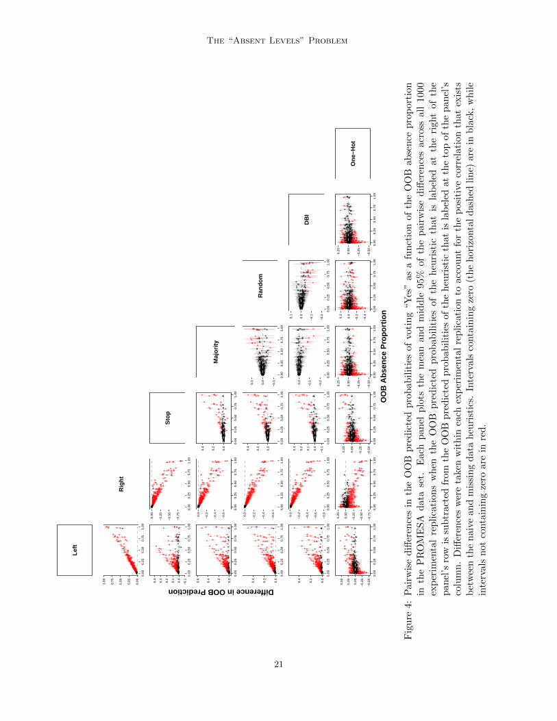
voting “Yes” for all possible pairwise combinations of the seven heuristics in Figure 4, whereeach panel plots the mean and middle 95% of these differences across all 1000 experimentalreplications as a function of the OOB absence proportion.

The large discrepancies in the predicted probabilities that are observed in Figure 4 are

particularly concerning since they can lead to different classifications. If we let y(h)nr denote

the OOB classification that a heuristic h makes for an observation n in an experimentalreplication r, then Cohen’s kappa coefficient (Cohen, 1960) provides one way of measuringthe level of agreement between two different heuristics h1, h2 ∈ H:

κ(h1,h2)r =

o(h1,h2)r − e(h1,h2)

r

1− e(h1,h2)r

, (14)

where

o(h1,h2)r =

1

N

N∑n=1

I(y(h1)nr = y(h2)

nr

)is the observed probability of agreement between the two heuristics, and where

e(h1,h2)r =

1

N2

K∑k=1

[(N∑

n=1

I(y(h1)nr = k

))·

(N∑

n=1

I(y(h2)nr = k

))]

is the expected probability of the two heuristics agreeing by chance. Therefore, within an

experimental replication r, we will observe κ(h1,h2)r = 1 if the two heuristics are in com-

plete agreement, and we will observe κ(h1,h2)r ≈ 0 if there is no agreement amongst the two

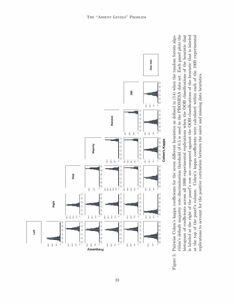
heuristics other than what would be expected by chance. In Figure 5, we plot histogramsof the Cohen’s kappa coefficient for all possible pairwise combinations of the seven heuris-tics across all 1000 experimental replications when the random forests algorithm’s defaultmajority vote discrimination threshold of 0.5 is used.

More generally, the areas underneath the receiver operating characteristic (ROC) andprecision-recall (PR) curves can be used to compare the overall performance of binaryclassifiers as the discrimination threshold is varied between 0 and 1. Specifically, as the dis-crimination threshold changes, the ROC curve plots the proportion of positive observationsthat a classifier correctly labels as a function of the proportion of negative observationsthat a classifier incorrectly labels, while the PR curve plots the proportion of a classifier’spositive labels that are truly positive as a function of the proportion of positive observationsthat a classifier correctly labels (Davis and Goadrich, 2006).

9This is the approach that is used by the randomForest R package. The scikit-learn Python moduleuses an alternative method of calculating the predicted response class probabilities which takes the averageof the predicted class probabilities over the trees in the random forest, where the predicted probability ofa response class k in an individual tree is estimated using the proportion of a node’s training samples thatbelong to the response class k.

22


Left

050100

150

0.5

0.6

0.7

0.8

0.9

1.0

Rig

ht

050100

150

0.5

0.6

0.7

0.8

0.9

1.0

050100

150

200

0.5

0.6

0.7

0.8

0.9

1.0

Sto

p

050100

150

0.5

0.6

0.7

0.8

0.9

1.0

050100

150

0.5

0.6

0.7

0.8

0.9

1.0

0

100

200

0.5

0.6

0.7

0.8

0.9

1.0

Maj

ority

050100

150

0.5

0.6

0.7

0.8

0.9

1.0

050100

150

200

0.5

0.6

0.7

0.8

0.9

1.0

050100

150

200

250

0.5

0.6

0.7

0.8

0.9

1.0

0

100

200

300

0.5

0.6

0.7

0.8

0.9

1.0

Ran

dom

050100

150

0.5

0.6

0.7

0.8

0.9

1.0

050100

150

0.5

0.6

0.7

0.8

0.9

1.0

0

100

200

300

400

0.5

0.6

0.7

0.8

0.9

1.0

0

100

200

300

400

0.5

0.6

0.7

0.8

0.9

1.0

0

100

200

300

0.5

0.6

0.7

0.8

0.9

1.0

DB

I

050100

0.5

0.6

0.7

0.8

0.9

1.0

050100

150

0.5

0.6

0.7

0.8

0.9

1.0

050100

150

0.5

0.6

0.7

0.8

0.9

1.0

050100

150

0.5

0.6

0.7

0.8

0.9

1.0

050100

150

0.5

0.6

0.7

0.8

0.9

1.0

050100

150

0.5

0.6

0.7

0.8

0.9

1.0

One

−Hot

Coh

en's

Kap

pa

Frequency

Fig

ure

5:

Pair

wis

eC

ohen

’ska

pp

aco

effici

ents

for

the

seven

diff

eren

th

euri

stic

sas

defi

ned

in(1

4)w

hen

the

ran

dom

fore

sts

algo

-ri

thm

’sd

efau

ltm

ajo

rity

vote

dis

crim

inat

ion

thre

shol

dof

0.5

isuse

din

the

PR

OM

ES

Ad

ata

set.

Eac

hp

anel

plo

tsth

eh

isto

gram

ofco

effici

ents

acro

ssal

l10

00ex

per

imen

tal

rep

lica

tion

sw

hen

the

OO

Bcl

assi

fica

tion

sof

the

heu

rist

icth

atis

lab

eled

at

the

right

of

the

pan

el’s

row

are

com

par

edag

ain

stth

eO

OB

clas

sifi

cati

ons

ofth

eh

euri

stic

that

isla

bel

edat

the

top

ofth

ep

an

el’s

colu

mn

.C

ohen

’ska

pp

aco

effici

ents

wer

eca

lcu

late

dw

ith

inea

chof

the

1000

exp

erim

enta

lre

pli

cati

on

sto

acco

unt

for

the

pos

itiv

eco

rrel

atio

nb

etw

een

the

nai

vean

dm

issi

ng

dat

ah

euri

stic

s.

23

Au

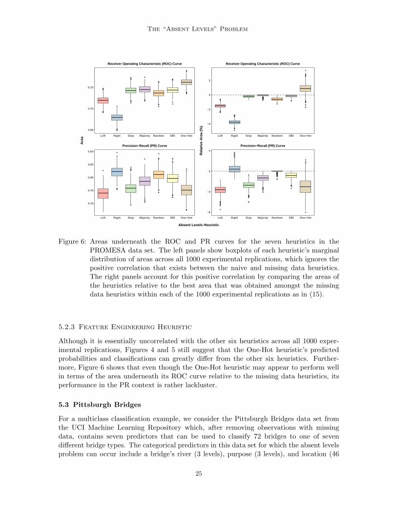
Taking the “Yes” vote to be the positive response class in our analysis, we calculate theareas underneath the ROC and PR curves for each heuristic h ∈ H within each experimentalreplication r. Boxplots depicting each heuristic’s marginal distribution of these two areasacross all 1000 experimental replications are shown in the left panels of Figure 6. However,these marginal boxplots ignore the positive correlation that exists between the naive andmissing data heuristics. Therefore, within every experimental replication r and similar towhat was previously done in our 1985 Auto Imports example, we also compare the areasfor each heuristic h ∈ H relative to the best area that was achieved amongst the missingdata heuristics Hm = {Stop,Majority,Random,DBI }:

AUC(h‖Hm)r =

AUC(h)r −maxh∈Hm AUC

(h)r

maxh∈Hm AUC(h)r

, (15)

where, depending on the context, AUC(h)r denotes the area that is underneath either the

ROC or PR curve for heuristic h in experimental replication r. Boxplots of these relativeareas across all 1000 experimental replications are displayed in the right panels of Figure 6.


As expected given our discussions in Section 3.2 and how we have chosen to index theresponse classes in our analysis, we see from Figure 4 that the Left heuristic results in sig-nificantly higher predicted probabilities of voting “Yes” than the other heuristics, while theRight heuristic yields predicted probabilities of voting “Yes” that are substantially lower.The consequences of this behavior in terms of making classifications can be observed inFigure 5, where we note that both the Left and Right heuristics tend to exhibit a high levelof disagreement when compared against any other heuristic’s classifications. Moreover, Fig-ure 6 illustrates that the randomForest R package’s practice of always sending absent levelsleft in binary classification is noticeably detrimental here—relative to the best performingmissing data heuristic, it gives areas underneath the ROC and PR curves that are, on av-erage, 1.5% and 3.7% worse, respectively. And although the Right heuristic appears to dowell in terms of the area underneath the PR curve, we once again emphasize the spuriousnature of this performance and caution against taking it at face value.


Similar to what was previously seen in our 1985 Auto Imports example, Figures 4 and 5show that the four missing data heuristics tend to exhibit a higher level of agreement withone another than they do with the Left, Right, and One-Hot heuristics. However, significantdifferences do still exist, and we see from Figure 6 that the relative performances of theheuristics will vary depending on the specific task at hand—the Majority heuristic slightlyoutperforms the three other missing data heuristics in terms of the area underneath theROC curve, while the Random heuristic does considerably better than all of its missingdata counterparts with respect to the area underneath the PR curve.

24


●

●

●

●

●●

●

●

●

●

●●

●

●

●

●

●

●

●

●●

●

●

●

●●

●

●

●

●

●●

●●

●

●

●

●●●●

●

0.68

0.70

0.72


Receiver Operating Characteristic (ROC) Curve

●

●

●

●

●

●

●●

●●

●

●

●

●

●

●

●

●●

●

●

●

●

●

●

●

●

●●

●

●

●

●

●

●●●

●

●

0.76

0.78

0.80

0.82

0.84


Precision−Recall (PR) Curve

Are

a

●●

●●●●

●●

●●

●●●

●

●

●●●●

●

●●

●

●

●

●●●●

●

●●

●●

●

●●●●●●

●

●●●

●

●

●●●●●●●●●●●●●●●●●

●

●●●●

●

●●●

●●●●

●●●●●

●

●●

●

●●

●

●

●

●

●

●

●

●

●

●

●

●●

●

−4

−2

0

2


Receiver Operating Characteristic (ROC) Curve

●

●

●

●

●

●

●●

●

●

●

●

●●

●

●●

●

●

●

●

●●●

●

●

●

●

●●●

●

●

●●●

●

●

●

●

●●●●●●●

●

●

●

●●

●

●

●

●●●

●

●

●

●●●

●

●

●

●●●

●●

●

●

●

●

●●

●

●●●●●

●●●

●

●

●

●●

●

●

●

●●●●

●

●●

●

●

●

●

●●●

●●

●

●

●

●

●●

●

●●●

●

●●

●

●

●

●●

●

●

●●

●●

●●

●

●

●

●

●

●

●●

●

●

●

●●●●●

●

●

●

●●●

●

●●●●

●●

●●

●

●

●●

●●

●●●

●

●

●

●

●●

●

●

●●●

●

●

●

●

●

●

●

−8

−4

0

4


Precision−Recall (PR) Curve

Rel

ativ

e A

rea

(%)


Figure 6: Areas underneath the ROC and PR curves for the seven heuristics in thePROMESA data set. The left panels show boxplots of each heuristic’s marginaldistribution of areas across all 1000 experimental replications, which ignores thepositive correlation that exists between the naive and missing data heuristics.The right panels account for this positive correlation by comparing the areas ofthe heuristics relative to the best area that was obtained amongst the missingdata heuristics within each of the 1000 experimental replications as in (15).


Although it is essentially uncorrelated with the other six heuristics across all 1000 exper-imental replications, Figures 4 and 5 still suggest that the One-Hot heuristic’s predictedprobabilities and classifications can greatly differ from the other six heuristics. Further-more, Figure 6 shows that even though the One-Hot heuristic may appear to perform wellin terms of the area underneath its ROC curve relative to the missing data heuristics, itsperformance in the PR context is rather lackluster.

5.3 Pittsburgh Bridges

For a multiclass classification example, we consider the Pittsburgh Bridges data set fromthe UCI Machine Learning Repository which, after removing observations with missingdata, contains seven predictors that can be used to classify 72 bridges to one of sevendifferent bridge types. The categorical predictors in this data set for which the absent levelsproblem can occur include a bridge’s river (3 levels), purpose (3 levels), and location (46

25

Au

levels). Consequently, recall from Section 3.2, that the random forests FORTRAN code andrandomForest R package will both employ an exhaustive search that always sends absentlevels right when splitting on either the river or purpose predictors, and that they willboth resort to using a random search that sends absent levels either left or right with equalprobability when splitting on the location predictor since it has too many levels for anexhaustive search to be computationally efficient. The OOB absence proportions for thisexample are summarized in the bottom panel of Figure 1 and in Table 1.

Within each experimental replication r, we can use the log loss

LogLoss(h)r = − 1

N

N∑n=1

K∑k=1

[I(yn = k) · log

(p(h)nkr

)]to evaluate the overall performance of each heuristic h ∈ H, where we once again let

p(h)nkr denote the OOB predicted probability that a heuristic h assigns to an observationn of belonging to a response class k in an experimental replication r. The left panel ofFigure 7 displays the marginal distribution of each heuristic’s log losses across all 1000experimental replications. However, to once again account for the positive correlation thatexists amongst the naive and missing data heuristics, within every experimental replicationr, we also compare the log losses for each heuristic h ∈ H relative to the best log loss thatwas achieved amongst the missing data heuristics Hm = {Stop,Majority,Random,DBI }:

LogLoss(h‖Hm)r =

LogLoss(h)r −minh∈Hm LogLoss

(h)r

minh∈Hm LogLoss(h)r

. (16)

Boxplots of these relative log losses are depicted in the right panel of Figure 7.


Although we once again stress the systematically biased nature of the Left and Right heuris-tics, we note from Figure 7 that the two naive heuristics are sometimes able to outperformthe missing data heuristics. Nevertheless, on average, the Left and Right heuristics resultedin log losses that are 0.7% and 1.9% worse than the best performing missing data heuristic,respectively.


Figure 7 shows that for this particular example, the Majority and Random heuristics per-form roughly on par with one another, and that they both also significantly outperformthe Stop and DBI heuristics—the smallest log loss amongst all of the missing data heuris-tics was achieved by either the Majority or the Random heuristic in 999 out of the 1000experimental replications.


It can also be observed from Figure 7 that, although the One-Hot heuristic can occasionallyoutperform the missing data heuristics, on average, it yields a log loss that is 4.5% worsethan the best performing missing data heuristic.

26


●●

●

●

●

●●

●

●

●

●

●

●

●

●

●

●●●

●

●

●

●

●

●

●

●●●

●

●

●

●

●

●

●

●●●

●

●

●

●

●●

●

●

●

●●●

●

●●●●

●

●

●●●

●

●●●●

●

●

●

●●

●

●

●

1.10

1.15

1.20

1.25

1.30

Left Right Stop Majority Random DBI OneHot

Log

Loss

●

●●●

●

●

●

●

●

●

●

●●●●

●

●

●

●●

●

●

●

●

●

●

●●●

●

●

●●

●

●

●●

●●

●

●●●

●●

●●

●

●

●

●●

●

●

●

●

●

●

●

●

●

●

●

●

●

●●●●●

●

●

●

●●●

●

●

●

●

●

●●

●

●●

●●●

●

●●

●

●

●

●●

●

●

●

●

●

●●●

●

●●

●

●●

●●●

●

●

●

●

●

●●●

●

●

●

●

●

●

●

●

●

●

0

5

10

15

Left Right Stop Majority Random DBI OneHot

Rel

ativ

e Lo

g Lo

ss (

%)


Figure 7: Log losses for the OOB predicted response class probabilities of the seven heuris-tics in the Pittsburgh Bridges data. The left panel shows boxplots of each heuris-tic’s marginal distribution of log losses set across all 1000 experimental replica-tions, which ignores the positive correlation that exists between the naive andmissing data heuristics. The right panel accounts for this positive correlation bycomparing the log losses of the heuristics relative to the best log loss that was ob-tained amongst the missing data heuristics within each of the 1000 experimentalreplications as in (16).

6. Conclusion

In this paper, we introduced and investigated the absent levels problem for decision treebased methods. In particular, by using Breiman and Cutler’s random forests FORTRAN codeand the randomForest R package as motivating case studies, we showed how overlooking theabsent levels problem could systematically bias a model. Furthermore, we presented threereal data examples which illustrated how absent levels can dramatically alter a model’sperformance in practice.

Even though a comprehensive theoretical analysis of the absent levels problem wasbeyond the scope of this paper, we empirically demonstrated how some simple heuristicscould be used to help mitigate the effects of absent levels. And although none of the missingdata and feature engineering heuristics that we considered performed uniformly better thanall of the others, they were all shown to be superior to the biased naive approaches thatare currently being employed due to oversights in the software implementations of decisiontree based methods.

Consequently, until a more robust theoretical solution is found, we encourage the soft-ware implementations which support the native categorical split capabilities of decision treesto incorporate the Random heuristic as a provisional measure given its reliability—in all ofour examples, the Random heuristic was always competitive in terms of its performance.Moreover, based on our own personal experiences, we note that the Random heuristic wasone of the easier heuristics to implement on top of the randomForest R package. In themeantime, while waiting for these mitigations to materialize, we also urge users who relyon decision tree based methods to feature engineer their data sets when possible in order tocircumvent the absent levels problem—although our empirical results suggest that this may

27

Au

sometimes be detrimental to a model’s performance, we believe this to still be preferableto the alternative of having to rely on biased approaches which do not adequately addressabsent levels.

Finally, although this paper primarily focused on the absent levels problem for randomforests and a particular subset of the types of analyses in which random forests have beenused, it is important to recognize that the issue of absent levels applies much more broadly.For example, decision tree based methods have also been employed for clustering, detectingoutliers, imputing missing values, and generating variable importance measures (Breiman,2003)—tasks which also depend on the terminal node behavior of the observations. In ad-dition, several extensions of decision tree based methods have been built on top of softwarewhich currently overlook absent levels—such as the quantile regression forests algorithm(Meinshausen, 2006, 2012) and the infinitesimal jackknife method for estimating the vari-ance of bagged predictors (Wager et al., 2014), which are both implemented on top of therandomForest R package. Indeed, given how extensively decision tree based methods havebeen used, a sizable number of these models have almost surely been significantly and un-knowingly affected by the absent levels problem in practice—further emphasizing the needfor the development of both theory and software that accounts for this issue.

Acknowledgements

The author is extremely grateful to Art Owen for numerous valuable discussions and in-sightful comments which substantially improved this paper. The author would also like tothank David Chan, Robert Bell, the action editor, and the anonymous reviewers for theirhelpful feedback. Finally, the author would like to thank Jim Koehler, Tim Hesterberg,Joseph Kelly, Ivan Dıaz, Jingang Miao, and Aiyou Chen for many interesting discussions.

References

Yali Amit and Donald Geman. Shape quantization and recognition with randomized trees.Neural Computation, 9:1545–1588, 1997.

Gerard Biau. Analysis of a random forests model. Journal of Machine Learning Research,13(1):1063–1095, 2012.

Gerard Biau, Luc Devroye, and Gabor Lugosi. Consistency of random forests and otheraveraging classifiers. Journal of Machine Learning Research, 9(1):2015–2033, 2008.

Leo Breiman. Bagging predictors. Machine Learning, 24(2):123–140, 1996a.

Leo Breiman. Out-of-bag estimation. Technical report, Department of Statistics, U.C.Berkeley, 1996b. URL https://www.stat.berkeley.edu/~breiman/OOBestimation.

pdf.

Leo Breiman. Random forests. Machine Learning, 45(1):5–32, 2001.

Leo Breiman. Manual—setting up, using, and understanding random forest v4.0. 2003.URL https://www.stat.berkeley.edu/~breiman/Using_random_forests_v4.0.pdf.

28

https://www.stat.berkeley.edu/~breiman/OOBestimation.pdf

https://www.stat.berkeley.edu/~breiman/OOBestimation.pdf

https://www.stat.berkeley.edu/~breiman/Using_random_forests_v4.0.pdf


Leo Breiman, Jerome. H. Friedman, Richard. A. Olshen, and Charles J. Stone. Classificationand Regression Trees. Wadsworth, 1984. ISBN 0-534-98053-8.

Jacob Cohen. A coefficient of agreement for nominal scales. Educational and PsychologicalMeasurement, 20:37–46, 1960.

Jesse Davis and Mark Goadrich. The relationship between precision-recall and ROC curves.In ICML ’06: Proceedings of the 23rd international conference on Machine learning, pages233–240, 2006.

Misha Denil, David Matheson, and Nando de Freitas. Narrowing the gap: Random forestsin theory and in practice. In Proceedings of the 31th International Conference on MachineLearning, pages 665–673, 2014.

Walter D. Fisher. On grouping for maximum homogeneity. Journal of the American Sta-tistical Association, 53(284):789–798, 1958.

Trevor J Hastie, Robert J. Tibshirani, and Jerome H. Friedman. The Elements of StatisticalLearning: Data Mining, Inference, and Prediction, Second Edition. Springer Series inStatistics. Springer, New York, 2009.

Tin Kam Ho. The random subspace method for constructing decision forests. IEEE Trans-actions on Pattern Analysis and Machine Intelligence, 20(8):832–844, 1998.

Torsten Hothorn and Achim Zeileis. partykit: A modular toolkit for recursive partytioningin R. Journal of Machine Learning Research, 16:3905–3909, 2015.

Torsten Hothorn, Kurt Hornik, and Achim Zeileis. Unbiased recursive partitioning: Aconditional inference framework. Journal of Computational and Graphical Statistics, 15(3):651–674, 2006.

Hemant Ishwaran, Udaya B. Kogalur, Eugene H. Blackstone, and Michael S. Lauer. Randomsurvival forests. Annals of Applied Statistics, 2(3):841–860, 2008.

Jeff Lewis. Rvoteview: Voteview Data in R, 2015. https://github.com/JeffreyBLewis/

Rvoteview, http://voteview.polisci.ucla.edu, http://voteview.com.

Andy Liaw and Matthew Wiener. Classification and regression by randomForest. R News,2(3):18–22, 2002.

Moshe Lichman. UCI machine learning repository, 2013. URL http://archive.ics.uci.

edu/ml.

Wei-Yin Loh and Nunta Vanichsetakul. Tree-structured classification via generalized dis-criminant analysis. Journal of the American Statistical Association, 83(403):715–725,1988.

Nolan M. McCarty, Keith T. Poole, and Howard Rosenthal. Income Redistribution andthe Realignment of American Politics. AEI Press, publisher for the American EnterpriseInstitute, 1997.

29

https://github.com/JeffreyBLewis/Rvoteview

https://github.com/JeffreyBLewis/Rvoteview

http://voteview.polisci.ucla.edu

http://voteview.com

http://archive.ics.uci.edu/ml

http://archive.ics.uci.edu/ml

Au

Nicolai Meinshausen. Quantile regression forests. Journal of Machine Learning Research,7:983–999, 2006.

Nicolai Meinshausen. quantregForest: Quantile Regression Forests, 2012. URL http://

CRAN.R-project.org/package=quantregForest. R package version 0.2-3.

Fabian Pedregosa, Gael Varoquaux, Alexandre Gramfort, Vincent Michel, BertrandThirion, Olivier Grisel, Mathieu Blondel, Peter Prettenhofer, Ron Weiss, VincentDubourg, Jake Vanderplas, Alexandre Passos, David Cournapeau, Matthieu Brucher,Matthieu Perrot, and Edouard Duchesnay. Scikit-learn: Machine learning in Python.Journal of Machine Learning Research, 12:2825–2830, 2011.

John R. Quinlan. C4.5: Programs for Machine Learning. Morgan Kaufmann PublishersInc., 1993.

Greg Ridgeway. gbm: Generalized Boosted Regression Models, 2013. URL http://CRAN.

R-project.org/package=gbm. R package version 2.1.

Brian D. Ripley. Pattern Recognition and Neural Networks. Cambridge University Press,Cambridge, 1996. ISBN 0-521-46086-7.

Maytal Saar-Tsechansky and Foster Provost. Handling missing values when applying clas-sification models. Journal of Machine Learning Research, 8:1623–1657, 2007.

Terry Therneau, Beth Atkinson, and Brian Ripley. rpart: Recursive Partitioning and Re-gression Trees, 2015. URL http://CRAN.R-project.org/package=rpart. R packageversion 4.1-10.

Stefan Wager, Trevor Hastie, and Bradley Efron. Confidence intervals for random forests:The jackknife and the infinitesimal jackknife. Journal of Machine Learning Research, 15(1):1625–1651, 2014.

30

http://CRAN.R-project.org/package=quantregForest

http://CRAN.R-project.org/package=quantregForest

http://CRAN.R-project.org/package=gbm

http://CRAN.R-project.org/package=gbm

http://CRAN.R-project.org/package=rpart

Date post:	06-Feb-2022
Category:	Documents
Upload:	others
View:	3 times
Download:	0 times

Absent Levels Problem

Documents