Southern Illinois University Edwardsville

Executive Summary Report

Lab Assignment #1

Forecasting Methods

IME-483 Production Planning And Control

By

Sumanth Bhavisetty

&

Khazi Mohammed Younus Abdul Ghani

Due Date: 09/29/2015

Team-D

Introduction:

The focus of the project is to determine the forecast of the given data using Excel and VBA, the very

first step is to figure out how to calculate forecasts in Excel‘s form without any manual calculations and then

provide the macros’ code of the excel calculations to the VBA format. According to the requirement of project,

demand is to be estimated using the following four methods, Moving Average Method, Exponential Smoothing

Method, Holt’s Method and Winter’s Method followed by calculating forecast errors for each method

respectively. The final step is to compare of all the above mentioned procedures using Mean Square Error

(MSE) method to identify the forecast that is most accurate to forecast demand. Main purpose is to find the

best method by comparing each method with its respective Minimum Square Error (MSE) value.

Purpose of the application:

The main objective of this project is to generate an interface application that provides ease of use for the

users to forecast demand in a simple way by entering the available data. To create this user interface, the

calculation part is done on Excel worksheets, this is where all the calculations work is done. Visual Basic

Application (VBA) is used to create an outer skin or interface over the excel worksheets to achieve desired

output, by doing simple tasks such as entering the data and to toggle between different methods by just

clicking on the buttons.

Methodology:

As mentioned above, 4 different methods are used to forecast demand based on set of given data. This is

a recorded data for demand per time period from previous years. Moving Average method is a simple and basic

calculation process to forecast demand. In this, the average of demand data is taken for desired time periods.

For moving average the equation used for the calculation is:

1Fall 2015

X t=[∑i=1

n

X t−i

n ]

This is a one step ahead forecast, this process fails in case of predicting demand for multi-step ahead

forecast. To refine this gap in forecasting we use Exponential Smoothing method. In this method, smoothing

constant (α) is used to forecast demand in a finer pattern. The following equations are used in Exponential

smoothing to forecast demand

Welcome Page:

2Fall 2015

X t=X t−1+α ( X t−1−X t−1 )

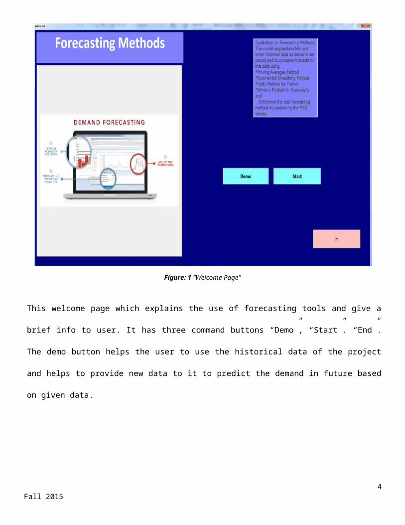
Figure: 1 “Welcome Page”

This welcome page which explains the use of forecasting tools and give a brief info to user. It has three

command buttons “Demo”, “Start”. “End”. The demo button helps the user to use the historical data of the

project and helps to provide new data to it to predict the demand in future based on given data.

Historical Data:

3Fall 2015

Figure: 2 “Historical Data”

After starting the program, the user will be able to input historical data which he/she needs to forecast.

Comparing Method Sheet:

4Fall 2015

Figure: 3 “Comparing Method”

In this page one can choose the forecasting method which they want to apply based on data with consideration

of different parameters which are involved in calculation. In addition to this, visual basic programming (VBA)

is used to evaluate the four methods and determine the best forecasting method based on which one resulted in

the lowest mean squared error (MSE).

The user is also able to view single graphs of the forecasting results or a compiled graph of all four methods as

shown below.

Moving average:

5Fall 2015

Figure: 4“Moving Average”

Exponential Smoothing:

6Fall 2015

Figure: 5 “Exponential Smoothing”

For Exponential Smoothing the equation used for the calculation is:

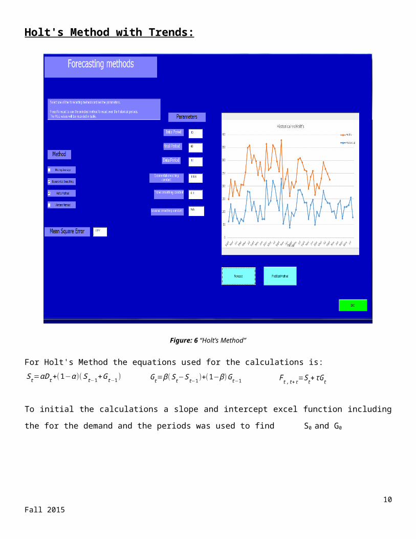
Holt's Method with Trends:

7Fall 2015

Figure: 6 “Holt’s Method”

For Holt's Method the equations used for the calculations is:

To initial the calculations a slope and intercept excel function including the for the demand and the periods was

used to find S0 and G0

Winter’s Method with Seasonality:

8Fall 2015

St=αDt+(1−α )(S t−1+Gt−1 ) Gt=β ( St−S t−1 )+(1−β )Gt−1 F t ,t +τ=St+τGt

Figure: 7 “Winters Method”

The equations used for the calculations is:

To calculate c t we used the way that explained in the class.

S0 & G0 is taken the same as Holt's Method then I did the calculation for all F t for regression from the

equation Ft,t+x = St +xGt by dividing Dt / F t than take the average for the periods that respectively meet

on the seasons then normalizing the values by the equation.

Best Method:

9Fall 2015

F t ,t +x=( St+xGt )ct+ x−NSt=α ( Y t

c t−N)+(1−α )(S t−1+Gt−1)Gt=β [ S t−St−1 ]+(1−β )Gt−1

Figure: 8 “Best Method”

In this page, you are able to compare the method and based on the MSE can have an accurate comparison as

which one has the minimum error and reliable calculation.

The Equations used for MSE calculation was

Conclusion:

Holt’s Method differentiates from Moving Average and Exponential Smoothing by simply adding the trend

factor inside forecasting. While Moving Average and Exponential Smoothing methods have only alpha

smoothing, it has also beta smoothing factor. Winter’s Method, above all; has also seasonal index which will

lead more precise forecasts (gamma).After using our program, expectedly, winter’s method provided the

minimum MSE. Therefore, winter’s Method is the best method in these four methods.

10Fall 2015

MSE=∑t=1

N

[Y ( t )−Y ( t ) ]2

N=

11Fall 2015