Deep Speech 2: End-to-End Speech Recognition in English and Mandarin Baidu Research – Silicon Valley AI Lab * Dario Amodei, Rishita Anubhai, Eric Battenberg, Carl Case, Jared Casper, Bryan Catanzaro, Jingdong Chen, Mike Chrzanowski, Adam Coates, Greg Diamos, Erich Elsen, Jesse Engel, Linxi Fan, Christopher Fougner, Tony Han, Awni Hannun, Billy Jun, Patrick LeGresley, Libby Lin, Sharan Narang, Andrew Ng, Sherjil Ozair, Ryan Prenger, Jonathan Raiman, Sanjeev Satheesh, David Seetapun, Shubho Sengupta, Yi Wang, Zhiqian Wang, Chong Wang, Bo Xiao, Dani Yogatama, Jun Zhan, Zhenyao Zhu Abstract We show that an end-to-end deep learning approach can be used to recognize either English or Mandarin Chinese speech—two vastly different languages. Be- cause it replaces entire pipelines of hand-engineered components with neural net- works, end-to-end learning allows us to handle a diverse variety of speech includ- ing noisy environments, accents and different languages. Key to our approach is our application of HPC techniques, resulting in a 7x speedup over our previous system [26]. Because of this efficiency, experiments that previously took weeks now run in days. This enables us to iterate more quickly to identify superior ar- chitectures and algorithms. As a result, in several cases, our system is competitive with the transcription of human workers when benchmarked on standard datasets. Finally, using a technique called Batch Dispatch with GPUs in the data center, we show that our system can be inexpensively deployed in an online setting, deliver- ing low latency when serving users at scale. 1 Introduction Decades worth of hand-engineered domain knowledge has gone into current state-of-the-art auto- matic speech recognition (ASR) pipelines. A simple but powerful alternative solution is to train such ASR models end-to-end, using deep learning to replace most modules with a single model [26]. We present the second generation of our speech system that exemplifies the major advantages of end- to-end learning. The Deep Speech 2 ASR pipeline approaches or exceeds the accuracy of Amazon Mechanical Turk human workers on several benchmarks, works in multiple languages with little modification, and is deployable in a production setting. It thus represents a significant step towards a single ASR system that addresses the entire range of speech recognition contexts handled by hu- mans. Since our system is built on end-to-end deep learning, we can employ a spectrum of deep learning techniques: capturing large training sets, training larger models with high performance computing, and methodically exploring the space of neural network architectures. We show that through these techniques we are able to reduce error rates of our previous end-to-end system [26] in English by up to 43%, and can also recognize Mandarin speech with high accuracy. One of the challenges of speech recognition is the wide range of variability in speech and acoustics. As a result, modern ASR pipelines are made up of numerous components including complex feature extraction, acoustic models, language and pronunciation models, speaker adaptation, etc. Build- ing and tuning these individual components makes developing a new speech recognizer very hard, especially for a new language. Indeed, many parts do not generalize well across environments or languages and it is often necessary to support multiple application-specific systems in order to pro- vide acceptable accuracy. This state of affairs is different from human speech recognition: people * Authorship order is alphabetical. 1 arXiv:1512.02595v1 [cs.CL] 8 Dec 2015
Transcript
Deep Speech 2: End-to-End Speech Recognition inEnglish and Mandarin
Baidu Research – Silicon Valley AI Lab∗Dario Amodei, Rishita Anubhai, Eric Battenberg, Carl Case, Jared Casper, Bryan Catanzaro,Jingdong Chen, Mike Chrzanowski, Adam Coates, Greg Diamos, Erich Elsen, Jesse Engel,
Linxi Fan, Christopher Fougner, Tony Han, Awni Hannun, Billy Jun, Patrick LeGresley,Libby Lin, Sharan Narang, Andrew Ng, Sherjil Ozair, Ryan Prenger, Jonathan Raiman,
Sanjeev Satheesh, David Seetapun, Shubho Sengupta, Yi Wang, Zhiqian Wang, Chong Wang,Bo Xiao, Dani Yogatama, Jun Zhan, Zhenyao Zhu
Abstract
We show that an end-to-end deep learning approach can be used to recognizeeither English or Mandarin Chinese speech—two vastly different languages. Be-cause it replaces entire pipelines of hand-engineered components with neural net-works, end-to-end learning allows us to handle a diverse variety of speech includ-ing noisy environments, accents and different languages. Key to our approach isour application of HPC techniques, resulting in a 7x speedup over our previoussystem [26]. Because of this efficiency, experiments that previously took weeksnow run in days. This enables us to iterate more quickly to identify superior ar-chitectures and algorithms. As a result, in several cases, our system is competitivewith the transcription of human workers when benchmarked on standard datasets.Finally, using a technique called Batch Dispatch with GPUs in the data center, weshow that our system can be inexpensively deployed in an online setting, deliver-ing low latency when serving users at scale.
1 Introduction
Decades worth of hand-engineered domain knowledge has gone into current state-of-the-art auto-matic speech recognition (ASR) pipelines. A simple but powerful alternative solution is to train suchASR models end-to-end, using deep learning to replace most modules with a single model [26]. Wepresent the second generation of our speech system that exemplifies the major advantages of end-to-end learning. The Deep Speech 2 ASR pipeline approaches or exceeds the accuracy of AmazonMechanical Turk human workers on several benchmarks, works in multiple languages with littlemodification, and is deployable in a production setting. It thus represents a significant step towardsa single ASR system that addresses the entire range of speech recognition contexts handled by hu-mans. Since our system is built on end-to-end deep learning, we can employ a spectrum of deeplearning techniques: capturing large training sets, training larger models with high performancecomputing, and methodically exploring the space of neural network architectures. We show thatthrough these techniques we are able to reduce error rates of our previous end-to-end system [26] inEnglish by up to 43%, and can also recognize Mandarin speech with high accuracy.
One of the challenges of speech recognition is the wide range of variability in speech and acoustics.As a result, modern ASR pipelines are made up of numerous components including complex featureextraction, acoustic models, language and pronunciation models, speaker adaptation, etc. Build-ing and tuning these individual components makes developing a new speech recognizer very hard,especially for a new language. Indeed, many parts do not generalize well across environments orlanguages and it is often necessary to support multiple application-specific systems in order to pro-vide acceptable accuracy. This state of affairs is different from human speech recognition: people
∗Authorship order is alphabetical.
1
arX
iv:1
512.
0259
5v1
[cs
.CL
] 8
Dec
201
5
have the innate ability to learn any language during childhood, using general skills to learn language.After learning to read and write, most humans can transcribe speech with robustness to variation inenvironment, speaker accent and noise, without additional training for the transcription task. Tomeet the expectations of speech recognition users, we believe that a single engine must learn to besimilarly competent; able to handle most applications with only minor modifications and able tolearn new languages from scratch without dramatic changes. Our end-to-end system puts this goalwithin reach, allowing us to approach or exceed the performance of human workers on several testsin two very different languages: Mandarin and English.
Since Deep Speech 2 (DS2) is an end-to-end deep learning system, we can achieve performancegains by focusing on three crucial components: the model architecture, large labeled trainingdatasets, and computational scale. This approach has also yielded great advances in other appli-cation areas such as computer vision and natural language. This paper details our contribution tothese three areas for speech recognition, including an extensive investigation of model architecturesand the effect of data and model size on recognition performance. In particular, we describe numer-ous experiments with neural networks trained with the Connectionist Temporal Classification (CTC)loss function [22] to predict speech transcriptions from audio. We consider networks composed ofmany layers of recurrent connections, convolutional filters, and nonlinearities, as well as the impactof a specific instance of Batch Normalization [63] (BatchNorm) applied to RNNs. We not onlyfind networks that produce much better predictions than those in previous work [26], but also findinstances of recurrent models that can be deployed in a production setting with no significant loss inaccuracy.
Beyond the search for better model architecture, deep learning systems benefit greatly from largequantities of training data. We detail our data capturing pipeline that has enabled us to create largerdatasets than what is typically used to train speech recognition systems. Our English speech systemis trained on 11,940 hours of speech, while the Mandarin system is trained on 9,400 hours. We usedata synthesis to further augment the data during training.
Training on large quantities of data usually requires the use of larger models. Indeed, our modelshave many more parameters than those used in our previous system. Training a single model atthese scales requires tens of exaFLOPs1 that would require 3-6 weeks to execute on a single GPU.This makes model exploration a very time consuming exercise, so we have built a highly optimizedtraining system that uses 8 or 16 GPUs to train one model. In contrast to previous large-scale trainingapproaches that use parameter servers and asynchronous updates [18, 10], we use synchronous SGD,which is easier to debug while testing new ideas, and also converges faster for the same degree ofdata parallelism. To make the entire system efficient, we describe optimizations for a single GPUas well as improvements to scalability for multiple GPUs. We employ optimization techniquestypically found in High Performance Computing to improve scalability. These optimizations includea fast implementation of the CTC loss function on the GPU, and a custom memory allocator. Wealso use carefully integrated compute nodes and a custom implementation of all-reduce to accelerateinter-GPU communication. Overall the system sustains approximately 50 teraFLOP/second whentraining on 16 GPUs. This amounts to 3 teraFLOP/second per GPU which is about 50% of peaktheoretical performance. This scalability and efficiency cuts training times down to 3 to 5 days,allowing us to iterate more quickly on our models and datasets.
We benchmark our system on several publicly available test sets and compare the results to ourprevious end-to-end system [26]. Our goal is to eventually reach human-level performance not onlyon specific benchmarks, where it is possible to improve through dataset-specific tuning, but on arange of benchmarks that reflects a diverse set of scenarios. To that end, we have also measuredthe performance of human workers on each benchmark for comparison. We find that our systemoutperforms humans in some commonly-studied benchmarks and has significantly closed the gap inmuch harder cases. In addition to public benchmarks, we show the performance of our Mandarinsystem on internal datasets that reflect real-world product scenarios.
Deep learning systems can be challenging to deploy at scale. Large neural networks are compu-tationally expensive to evaluate for each user utterance, and some network architectures are moreeasily deployed than others. Through model exploration, we find high-accuracy, deployable net-work architectures, which we detail here. We also employ a batching scheme suitable for GPU
11 exaFLOP = 1018 FLoating-point OPerations.
2
hardware called Batch Dispatch that leads to an efficient, real-time implementation of our Mandarinengine on production servers. Our implementation achieves a 98th percentile compute latency of 67milliseconds, while the server is loaded with 10 simultaneous audio streams.
The remainder of the paper is as follows. We begin with a review of related work in deep learning,end-to-end speech recognition, and scalability in Section 2. Section 3 describes the architectural andalgorithmic improvements to the model and Section 4 explains how to efficiently compute them. Wediscuss the training data and steps taken to further augment the training set in Section 5. An analysisof results for the DS2 system in English and Mandarin is presented in Section 6. We end with adescription of the steps needed to deploy DS2 to real users in Section 7.
2 Related Work
This work is inspired by previous work in both deep learning and speech recognition. Feed-forwardneural network acoustic models were explored more than 20 years ago [7, 50, 19]. Recurrent neu-ral networks and networks with convolution were also used in speech recognition around the sametime [51, 67]. More recently DNNs have become a fixture in the ASR pipeline with almost allstate of the art speech work containing some form of deep neural network [42, 29, 17, 16, 43, 58].Convolutional networks have also been found beneficial for acoustic models [1, 53]. Recurrentneural networks, typically LSTMs, are just beginning to be deployed in state-of-the art recogniz-ers [24, 25, 55] and work well together with convolutional layers for the feature extraction [52].Models with both bidirectional [24] and unidirectional recurrence have been explored as well.
End-to-end speech recognition is an active area of research, showing compelling results when usedto re-score the outputs of a DNN-HMM [23] and standalone [26]. Two methods are currently used tomap variable length audio sequences directly to variable length transcriptions. The RNN encoder-decoder paradigm uses an encoder RNN to map the input to a fixed length vector and a decodernetwork to expand the fixed length vector into a sequence of output predictions [11, 62]. Adding anattentional mechanism to the decoder greatly improves performance of the system, particularly withlong inputs or outputs [2]. In speech, the RNN encoder-decoder with attention performs well bothin predicting phonemes [12] or graphemes [3, 8].
The other commonly used technique for mapping variable length audio input to variable lengthoutput is the CTC loss function [22] coupled with an RNN to model temporal information. The CTC-RNN model performs well in end-to-end speech recognition with grapheme outputs [23, 27, 26, 40].The CTC-RNN model has also been shown to work well in predicting phonemes [41, 54], thougha lexicon is still needed in this case. Furthermore it has been necessary to pre-train the CTC-RNNnetwork with a DNN cross-entropy network that is fed frame-wise alignments from a GMM-HMMsystem [54]. In contrast, we train the CTC-RNN networks from scratch without the need of frame-wise alignments for pre-training.
Exploiting scale in deep learning has been central to the success of the field thus far [36, 38]. Train-ing on a single GPU resulted in substantial performance gains [49], which were subsequently scaledlinearly to two [36] or more GPUs [15]. We take advantage of work in increasing individual GPUefficiency for low-level deep learning primitives [9]. We build on the past work in using model-parallelism [15], data-parallelism [18] or a combination of the two [64, 26] to create a fast andhighly scalable system for training deep RNNs in speech recognition.
Data has also been central to the success of end-to-end speech recognition, with over 7000 hoursof labeled speech used in Deep Speech 1 (DS1) [26]. Data augmentation has been highly effectivein improving the performance of deep learning in computer vision [39, 56, 14]. This has also beenshown to improve speech systems [21, 26]. Techniques used for data augmentation in speech rangefrom simple noise addition [26] to complex perturbations such as simulating changes to the vocaltract length and rate of speech of the speaker [31, 35].
Existing speech systems can also be used to bootstrap new data collection. In one approach, theauthors use one speech engine to align and filter a thousand hours of read speech [46]. In anotherapproach, a heavy-weight offline speech recognizer is used to generate transcriptions for tens ofthousands of hours of speech [33]. This is then passed through a filter and used to re-train the recog-nizer, resulting in significant performance gains. We draw inspiration from these past approaches in
3
bootstrapping larger datasets and data augmentation to increase the effective amount of labeled datafor our system.
3 Model Architecture
A simple multi-layer model with a single recurrent layer cannot exploit thousands of hours of la-belled speech. In order to learn from datasets this large, we increase the model capacity via depth.We explore architectures with up to 11 layers including many bidirectional recurrent layers and con-volutional layers. These models have nearly 8 times the amount of computation per data example asthe models in Deep Speech 1 making fast optimization and computation critical. In order to optimizethese models successfully, we use Batch Normalization for RNNs and a novel optimization curricu-lum we call SortaGrad. We also exploit long strides between RNN inputs to reduce computationper example by a factor of 3. This is helpful for both training and evaluation, though requires somemodifications in order to work well with CTC. Finally, though many of our research results makeuse of bidirectional recurrent layers, we find that excellent models exist using only unidirectionalrecurrent layers—a feature that makes such models much easier to deploy. Taken together thesefeatures allow us to tractably optimize deep RNNs and improve performance by more than 40% inboth English and Mandarin error rates over the smaller baseline models.
3.1 Preliminaries
Figure 1 shows the architecture of the DS2 system which at its core is similar to the previous DS1system [26]: a recurrent neural network (RNN) trained to ingest speech spectrograms and generatetext transcriptions.
Let a single utterance x(i) and label y(i) be sampled from a training set X ={(x(1), y(1)), (x(2), y(2)), . . .}. Each utterance, x(i), is a time-series of length T (i) where everytime-slice is a vector of audio features, x(i)t , t = 0, . . . ,T (i) − 1. We use a spectrogram of powernormalized audio clips as the features to the system, so x(i)t,p denotes the power of the p’th frequencybin in the audio frame at time t. The goal of the RNN is to convert an input sequence x(i) into afinal transcription y(i). For notational convenience, we drop the superscripts and use x to denote achosen utterance and y the corresponding label.
The outputs of the network are the graphemes of each language. At each output time-step t, the RNNmakes a prediction over characters, p(`t|x), where `t is either a character in the alphabet or the blanksymbol. In English we have `t ∈ {a, b, c, . . . , z, space, apostrophe, blank}, where we have addedthe apostrophe as well as a space symbol to denote word boundaries. For the Mandarin system thenetwork outputs simplified Chinese characters. We describe this in more detail in Section 3.9.
The RNN model is composed of several layers of hidden units. The architectures we experimentwith consist of one or more convolutional layers, followed by one or more recurrent layers, followedby one or more fully connected layers.
The hidden representation at layer l is given by hl with the convention that h0 represents the inputx. The bottom of the network is one or more convolutions over the time dimension of the input. Fora context window of size c, the i-th activation at time-step t of the convolutional layer is given by
hlt,i = f(wli ◦ hl−1t−c:t+c) (1)
where ◦ denotes the element-wise product between the i-th filter and the context window of theprevious layers activations, and f denotes a unary nonlinear function. We use the clipped rectified-linear (ReLU) function σ(x) = min{max{x, 0}, 20} as our nonlinearity. In some layers, usuallythe first, we sub-sample by striding the convolution by s frames. The goal is to shorten the numberof time-steps for the recurrent layers above.
Following the convolutional layers are one or more bidirectional recurrent layers [57]. The forwardin time
−→h l and backward in time
←−h l recurrent layer activations are computed as−→h lt = g(hl−1t ,
−→h lt−1)
←−h lt = g(hl−1t ,
←−h lt+1)
(2)
4
CTC
Spectrogram
Recurrentor
GRU(Bidirectional)
1D or 2DInvariant
Convolution
Fully Connected
BatchNormalization
Figure 1: Architecture of the DS2 system used to train on both English and Mandarin speech. We explorevariants of this architecture by varying the number of convolutional layers from 1 to 3 and the number ofrecurrent or GRU layers from 1 to 7.
The two sets of activations are summed to form the output activations for the layer hl =−→h l +
←−h l.
The function g(·) can be the standard recurrent operation
−→h lt = f(W lhl−1t +
−→U l−→h lt−1 + bl) (3)
where W l is the input-hidden weight matrix,−→U l is the recurrent weight matrix and bl is a bias term.
In this case the input-hidden weights are shared for both directions of the recurrence. The functiong(·) can also represent more complex recurrence operations such as the Long Short-Term Memory(LSTM) units [30] and the gated recurrent units (GRU) [11].
After the bidirectional recurrent layers we apply one or more fully connected layers with
hlt = f(W lhl−1t + bl) (4)
The output layer L is a softmax computing a probability distribution over characters given by
p(`t = k|x) = exp(wLk · hL−1t )∑j exp(w
Lj · hL−1t )
(5)
The model is trained using the CTC loss function [22]. Given an input-output pair (x, y) and thecurrent parameters of the network θ, we compute the loss function L(x, y; θ) and its derivative withrespect to the parameters of the network ∇θL(x, y; θ). This derivative is then used to update thenetwork parameters through the backpropagation through time algorithm.
In the following subsections we describe the architectural and algorithmic improvements made rel-ative to DS1 [26]. Unless otherwise stated these improvements are language agnostic. We reportresults on an English speaker held out development set which is an internal dataset containing 2048utterances of primarily read speech. All models are trained on datasets described in Section 5.We report Word Error Rate (WER) for the English system and Character Error Rate (CER) for theMandarin system. In both cases we integrate a language model in a beam search decoding step asdescribed in Section 3.8.
5
Architecture Hidden Units Train Dev
Baseline BatchNorm Baseline BatchNorm
1 RNN, 5 total 2400 10.55 11.99 13.55 14.403 RNN, 5 total 1880 9.55 8.29 11.61 10.565 RNN, 7 total 1510 8.59 7.61 10.77 9.787 RNN, 9 total 1280 8.76 7.68 10.83 9.52
Table 1: Comparison of WER on a training and development set for various depths of RNN, with and withoutBatchNorm. The number of parameters is kept constant as the depth increases, thus the number of hidden unitsper layer decreases. All networks have 38 million parameters. The architecture “M RNN, N total” implies 1layer of 1D convolution at the input, M consecutive bidirectional RNN layers, and the rest as fully-connectedlayers with N total layers in the network.
3.2 Batch Normalization for Deep RNNs
To efficiently scale our model as we scale the training set, we increase the depth of the networks byadding more hidden layers, rather than making each layer larger. Previous work has examined doingso by increasing the number of consecutive bidirectional recurrent layers [24]. We explore BatchNormalization (BatchNorm) as a technique to accelerate training for such networks [63] since theyoften suffer from optimization issues.
Recent research has shown that BatchNorm improves the speed of convergence of recurrent nets,without showing any improvement in generalization performance [37]. In contrast, we demonstratethat when applied to very deep networks of simple RNNs on large data sets, batch normalizationsubstantially improves final generalization error while greatly accelerating training.
In a typical feed-forward layer containing an affine transformation followed by a non-linearity f(·),we insert a BatchNorm transformation by applying f(B(Wh)) instead of f(Wh+ b), where
B(x) = γx− E[x]
(Var[x] + ε)1/2
+ β. (6)
The terms E and Var are the empirical mean and variance over a minibatch. The bias b of thelayer is dropped since its effect is cancelled by mean removal. The learnable parameters γ and βallow the layer to scale and shift each hidden unit as desired. The constant ε is small and positive,and is included only for numerical stability. In our convolutional layers the mean and varianceare estimated over all the temporal output units for a given convolutional filter on a minibatch.The BatchNorm transformation reduces internal covariate shift by insulating a given layer frompotentially uninteresting changes in the mean and variance of the layer’s input.
We consider two methods of extending BatchNorm to bidirectional RNNs [37]. A natural extensionis to insert a BatchNorm transformation immediately before every non-linearity. Equation 3 thenbecomes −→
h lt = f(B(W lhl−1t +−→U l−→h lt−1)). (7)
In this case the mean and variance statistics are accumulated over a single time-step of the minibatch.The sequential dependence between time-steps prevents averaging over all time-steps. We find thatthis technique does not lead to improvements in optimization. We also tried accumulating an averageover successive time-steps, so later time-steps are normalized over all present and previous time-steps. This also proved ineffective and greatly complicated backpropagation.
We find that sequence-wise normalization [37] overcomes these issues. The recurrent computationis given by −→
h lt = f(B(W lhl−1t ) +−→U l−→h lt−1). (8)
For each hidden unit, we compute the mean and variance statistics over all items in the minibatchover the length of the sequence. Figure 2 shows that deep networks converge faster with sequence-wise normalization. Table 1 shows that the performance improvement from sequence-wise normal-ization increases with the depth of the network, with a 12% performance difference for the deepestnetwork. When comparing depth, in order to control for model size we hold constant the total
6
50 100 150 200 250 300
Iteration (⇥103)
20
30
40
50
60
Cos
t
5-1 BN5-1 No BN9-7 BN9-7 No BN
Figure 2: Training curves of two models trained with and without BatchNorm. We start the plot after the firstepoch of training as the curve is more difficult to interpret due to the SortaGrad curriculum method mentionedin Section 3.3
Train Dev
Baseline BatchNorm Baseline BatchNorm
Not Sorted 10.71 8.04 11.96 9.78Sorted 8.76 7.68 10.83 9.52
Table 2: Comparison of WER on a training and development set with and without SortaGrad, and with andwithout batch normalization.
number of parameters and still see strong performance gains. We would expect to see even largerimprovements from depth if we held constant the number of activations per layer and added lay-ers. We also find that BatchNorm harms generalization error for the shallowest network just as itconverges slower for shallower networks.
The BatchNorm approach works well in training, but is difficult to implement for a deployed ASRsystem, since it is often necessary to evaluate a single utterance in deployment rather than a batch.We find that normalizing each neuron to its mean and variance over just the sequence degradesperformance. Instead, we store a running average of the mean and variance for the neuron collectedduring training, and use these for evaluation in deployment [63]. Using this technique, we canevaluate a single utterance at a time with better results than evaluating with a large batch.
3.3 SortaGrad
Training on examples of varying length pose some algorithmic challenges. One possible solution istruncating backpropagation through time [68], so that all examples have the same sequence lengthduring training [52]. However, this can inhibit the ability to learn longer term dependencies. Otherworks have found that presenting examples in order of difficulty can accelerate online learning [6,70]. A common theme in many sequence learning problems including machine translation andspeech recognition is that longer examples tend to be more challenging [11].
The CTC cost function that we use implicitly depends on the length of the utterance,
L(x, y; θ) = − log∑
`∈Align(x,y)
T∏t
pctc(`t|x; θ). (9)
where Align(x, y) is the set of all possible alignments of the characters of the transcription y toframes of input x under the CTC operator. In equation 9, the inner term is a product over time-stepsof the sequence, which shrinks with the length of the sequence since pctc(`t|x; θ) < 1. This moti-vates a curriculum learning strategy we title SortaGrad. SortaGrad uses the length of the utteranceas a heuristic for difficulty, since long utterances have higher cost than short utterances.
Table 3: Comparison of development set WER for networks with either simple RNN or GRU, for variousdepths. All models have batch normalization, one layer of 1D-invariant convolution, and approximately 38million parameters.
In the first training epoch, we iterate through the training set in increasing order of the length ofthe longest utterance in the minibatch. After the first epoch, training reverts back to a random orderover minibatches. Table 2 shows a comparison of training cost with and without SortaGrad on the9 layer model with 7 recurrent layers. This effect is particularly pronounced for networks withoutBatchNorm, since they are numerically less stable. In some sense the two techniques substitute forone another, though we still find gains when applying SortaGrad and BatchNorm together. Evenwith BatchNorm we find that this curriculum improves numerical stability and sensitivity to smallchanges in training. Numerical instability can arise from different transcendental function imple-mentations in the CPU and the GPU, especially when computing the CTC cost. This curriculumgives comparable results for both implementations.
We suspect that these benefits occur primarily because long utterances tend to have larger gradients,yet we use a fixed learning rate independent of utterance length. Furthermore, longer utterances aremore likely to cause the internal state of the RNNs to explode at an early stage in training.
3.4 Comparison of simple RNNs and GRUs
The models we have shown so far are simple RNNs that have bidirectional recurrent layers with therecurrence for both the forward in time and backward in time directions modeled by Equation 3.Current research in speech and language processing has shown that having a more complex re-currence can allow the network to remember state over more time-steps while making them morecomputationally expensive to train [52, 8, 62, 2]. Two commonly used recurrent architectures are theLong Short-Term Memory (LSTM) units [30] and the Gated Recurrent Units (GRU) [11], thoughmany other variations exist. A recent comprehensive study of thousands of variations of LSTM andGRU architectures showed that a GRU is comparable to an LSTM with a properly initialized forgetgate bias, and their best variants are competitive with each other [32]. We decided to examine GRUsbecause experiments on smaller data sets showed the GRU and LSTM reach similar accuracy forthe same number of parameters, but the GRUs were faster to train and less likely to diverge.
The GRUs we use are computed by
zt = σ(Wzxt + Uzht−1 + bz)
rt = σ(Wrxt + Urht−1 + br)
ht = f(Whxt + rt ◦ Uhht−1 + bh)
ht = (1− zt)ht−1 + ztht
(10)
where σ(·) is the sigmoid function, z and r represent the update and reset gates respectively, andwe drop the layer superscripts for simplicity. We differ slightly from the standard GRU in that wemultiply the hidden state ht−1 by Uh prior to scaling by the reset gate. This allows for all operationson ht−1 to be computed in a single matrix multiplication. The output nonlinearity f(·) is typicallythe hyperbolic tangent function tanh. However, we find similar performance for tanh and clipped-ReLU nonlinearities and choose to use the clipped-ReLU for simplicity and uniformity with the restof the network.
Both GRU and simple RNN architectures benefit from batch normalization and show strong re-sults with deep networks. However, Table 3 shows that for a fixed number of parameters, the GRUarchitectures achieve better WER for all network depths. This is clear evidence of the long termdependencies inherent in the speech recognition task present both within individual words and be-
8
Architecture Channels Filter dimension Stride Regular Dev Noisy Dev
Table 4: Comparison of WER for various arrangements of convolutional layers. In all cases, the convolutionsare followed by 7 recurrent layers and 1 fully connected layer. For 2D-invariant convolutions the first dimen-sion is frequency and the second dimension is time. All models have BatchNorm, SortaGrad, and 35 millionparameters.
tween words. As we discuss in Section 3.8, even simple RNNs are able to implicitly learn a languagemodel due to the large amount of training data. Interestingly, the GRU networks with 5 or more re-current layers do not significantly improve performance. We attribute this to the thinning from 1728hidden units per layer for 1 recurrent layer to 768 hidden units per layer for 7 recurrent layers, tokeep the total number of parameters constant.
The GRU networks outperform the simple RNNs in Table 3. However, in later results (Section 6) wefind that as we scale up the model size, for a fixed computational budget the simple RNN networksperform slightly better. Given this, most of the remaining experiments use the simple RNN layersrather than the GRUs.
3.5 Frequency Convolutions
Temporal convolution is commonly used in speech recognition to efficiently model temporal trans-lation invariance for variable length utterances. This type of convolution was first proposed forneural networks in speech more than 25 years ago [67]. Many neural network speech models have afirst layer that processes input frames with some context window [16, 66]. This can be viewed as atemporal convolution with a stride of one.
Additionally, sub-sampling is essential to make recurrent neural networks computationally tractablewith high sample-rate audio. The DS1 system accomplished this through the use of a spectrogramas input and temporal convolution in the first layer with a stride parameter to reduce the number oftime-steps [26].
Convolutions in frequency and time domains, when applied to the spectral input features prior toany other processing, can slightly improve ASR performance [1, 53, 60]. Convolution in frequencyattempts to model spectral variance due to speaker variability more concisely than what is pos-sible with large fully connected networks. Since spectral ordering of features is removed by fully-connected and recurrent layers, frequency convolutions work better as the first layers of the network.
We experiment with adding between one and three layers of convolution. These are both in the time-and-frequency domain (2D invariance) and in the time-only domain (1D invariance). In all cases weuse a same convolution, preserving the number of input features in both frequency and time. Insome cases, we specify a stride across either dimension which reduces the size of the output. We donot explicitly control for the number of parameters, since convolutional layers add a small fractionof parameters to our networks. All networks shown in Table 4 have about 35 million parameters.
We report results on two datasets—a development set of 2048 utterances (“Regular Dev”) and amuch noisier dataset of 2048 utterances (“Noisy Dev”) randomly sampled from the CHiME 2015development datasets [4]. We find that multiple layers of 1D-invariant convolutions provides a verysmall benefit. The 2D-invariant convolutions improve results substantially on noisy data, whileproviding a small benefit on clean data. The change from one layer of 1D-invariant convolution tothree layers of 2D-invariant convolution improves WER by 23.9% on the noisy development set.
Table 5: Comparison of WER with different amounts of striding for unigram and bigram outputs on a modelwith 1 layer of 1D-invariant convolution, 7 recurrent layers, and 1 fully connected layer. All models haveBatchNorm, SortaGrad, and 35 million parameters. The models are compared on a development set with andwithout the use of a 5-gram language model.
3.6 Striding
In the convolutional layers, we apply a longer stride and wider context to speed up training as fewertime-steps are required to model a given utterance. Downsampling the input sound (through FFT andconvolutional striding) reduces the number of time-steps and computation required in the followinglayers, but at the expense of reduced performance.
In our Mandarin models, we employ striding in the straightforward way. However, in English,striding can reduce accuracy simply because the output of our network requires at least one time-step per output character, and the number of characters in English speech per time-step is highenough to cause problems when striding2. To overcome this, we can enrich the English alphabetwith symbols representing alternate labellings like whole words, syllables or non-overlapping n-grams. In practice, we use non-overlapping bi-graphemes or bigrams, since these are simple toconstruct, unlike syllables, and there are few of them compared to alternatives such as whole words.We transform unigram labels into bigram labels through a simple isomorphism.
Non-overlapping bigrams shorten the length of the output transcription and thus allow for a decreasein the length of the unrolled RNN. The sentence the cat sat with non-overlapping bigrams is seg-mented as [th, e, space, ca, t, space, sa, t]. Notice that for words with odd number of characters, thelast character becomes an unigram and space is treated as an unigram as well. This isomorphismensures that the same words are always composed of the same bigram and unigram tokens. Theoutput set of bigrams consists of all bigrams that occur in the training set.
In Table 5 we show results for both the bigram and unigram systems for various levels of striding,with or without a language model. We observe that bigrams allow for larger strides without anysacrifice in in the word error rate. This allows us to reduce the number of time-steps of the unrolledRNN benefiting both computation and memory usage.
3.7 Row Convolution and Unidirectional Models
Bidirectional RNN models are challenging to deploy in an online, low-latency setting, because theyare built to operate on an entire sample, and so it is not possible to perform the transcription processas the utterance streams from the user. We have found an unidirectional architecture that performsas well as our bidirectional models. This allows us to use unidirectional, forward-only RNN layersin our deployment system.
To accomplish this, we employ a special layer that we call row convolution, shown in Figure 3. Theintuition behind this layer is that we only need a small portion of future information to make anaccurate prediction at the current time-step. Suppose at time-step t, we use a future context of τsteps. We now have a feature matrix ht:t+τ = [ht,ht+1, ...,ht+τ ] of size d × (τ + 1). We define aparameter matrix W of the same size as ht:t+τ . The activations rt for the new layer at time-step tare
2Chinese characters are more similar to English syllables than English characters. This is reflected in ourtraining data, where there are on average 14.1 characters/s in English, while only 3.3 characters/s in Mandarin.Conversely, the Shannon entropy per character as calculated from occurrence in the training set, is less inEnglish due to the smaller character set—4.9 bits/char compared to 12.6 bits/char in Mandarin. This impliesthat spoken Mandarin has a lower temporal entropy density, ∼41 bits/s compared to ∼58 bits/s, and can thusmore easily be temporally compressed without losing character information.
10
Recurrent layer
Row conv layer
ht ht+1 ht+2 ht+3
rt+3rt+2rt+1rt
Figure 3: Row convolution architecture with future context size of 2
rt,i =
τ+1∑j=1
Wi,jht+j−1,i, for 1 ≤ i ≤ d. (11)
Since the convolution-like operation in Eq. 11 is row oriented for both W and ht:t+τ , we call thislayer row convolution.
We place the row convolution layer above all recurrent layers. This has two advantages. First, thisallows us to stream all computation below the row convolution layer on a finer granularity given littlefuture context is needed. Second, this results in better CER compared to the best bidirectional modelfor Mandarin. We conjecture that the recurrent layers have learned good feature representations,so the row convolution layer simply gathers the appropriate information to feed to the classifier.Results for a unidirectional Mandarin speech system with row convolution and a comparison to abidirectional model are given in Section 7 on deployment.
3.8 Language Model
We train our RNN Models over millions of unique utterances, which enables the network to learn apowerful implicit language model. Our best models are quite adept at spelling, without any externallanguage constraints. Further, in our development datasets we find many cases where our models canimplicitly disambiguate homophones—for example, “he expects the Japanese agent to sell it for twohundred seventy five thousand dollars”. Nevertheless, the labeled training data is small comparedto the size of unlabeled text corpora that are available. Thus we find that WER improves when wesupplement our system with a language model trained from external text.
We use an n-gram language model since they scale well to large amounts of unlabeled text [26].For English, our language model is a Kneser-Ney smoothed 5-gram model with pruning that istrained using the KenLM toolkit [28] on cleaned text from the Common Crawl Repository3. Thevocabulary is the most frequently used 400,000 words from 250 million lines of text, which producesa language model with about 850 million n-grams. For Mandarin, the language model is a Kneser-Ney smoothed character level 5-gram model with pruning that is trained on an internal text corpusof 8 billion lines of text. This produces a language model with about 2 billion n-grams.
During inference we search for the transcription y that maximizes Q(y) shown in Equation 12. Thisis a linear combination of log probabilities from the CTC trained network and language model, alongwith a word insertion term [26].
The weight α controls the relative contributions of the language model and the CTC network. Theweight β encourages more words in the transcription. These parameters are tuned on a developmentset. We use a beam search to find the optimal transcription [27].
Table 6: Comparison of WER for English and CER for Mandarin with and without a language model. Theseare simple RNN models with only one layer of 1D invariant convolution.
Table 6 shows that an external language model helps both English and Mandarin speech systems.The relative improvement given by the language model drops from 48% to 36% in English and 27%to 23% in Mandarin, as we go from a model with 5 layers and 1 recurrent layer to a model with 9layers and 7 recurrent layers. We hypothesize that the network builds a stronger implicit languagemodel with more recurrent layers.
The relative performance improvement from a language model is higher in English than in Mandarin.We attribute this to the fact that a Chinese character represents a larger block of information thanan English character. For example, if we output directly to syllables or words in English, the modelwould make fewer spelling mistakes and the language model would likely help less.
3.9 Adaptation to Mandarin
The techniques that we have described so far can be used to build an end-to-end Mandarin speechrecognition system that outputs Chinese characters directly. This precludes the need to construct apronunciation model, which is often a fairly involved component for porting speech systems to otherlanguages [59]. Direct output to characters also precludes the need to explicitly model languagespecific pronunciation features. For example we do not need to model Mandarin tones explicitly, assome speech systems must do [59, 45].
The only architectural changes we make to our networks are due to the characteristics of the Chinesecharacter set. Firstly, the output layer of the network outputs about 6000 characters, which includesthe Roman alphabet, since hybrid Chinese-English transcripts are common. We incur an out ofvocabulary error at evaluation time if a character is not contained in this set. This is not a majorconcern, as our test set has only 0.74% out of vocab characters.
We use a character level language model in Mandarin as words are not usually segmented in text.The word insertion term of Equation 12 becomes a character insertion term. In addition, we find thatthe performance of the beam search during decoding levels off at a smaller beam size. This allowsus to use a beam size of 200 with a negligible degradation in CER. In Section 6.2, we show thatour Mandarin speech models show roughly the same improvements to architectural changes as ourEnglish speech models.
4 System Optimizations
Our networks have tens of millions of parameters, and the training algorithm takes tens of single-precision exaFLOPs to converge. Since our ability to evaluate hypotheses about our data and mod-els depends on the ability to train models quickly, we built a highly optimized training system.This system has two main components—a deep learning library written in C++, along with a high-performance linear algebra library written in both CUDA and C++. Our optimized software, runningon dense compute nodes with 8 Titan X GPUs per node, allows us to sustain 24 single-precisionteraFLOP/second when training a single model on one node. This is 45% of the theoretical peakcomputational throughput of each node. We also can scale to multiple nodes, as outlined in the nextsubsection.
4.1 Scalability and Data-Parallelism
We use the standard technique of data-parallelism to train on multiple GPUs using synchronousSGD. Our most common configuration uses a minibatch of 512 on 8 GPUs. Our training pipeline
12
binds one process to each GPU. These processes then exchange gradient matrices during the back-propagation by using all-reduce, which exchanges a matrix between multiple processes and sumsthe result so that at the end, each process has a copy of the sum of all matrices from all processes.
We find synchronous SGD useful because it is reproducible and deterministic. We have foundthat the appearance of non-determinism in our system often signals a serious bug, and so havingreproducibility as a goal has greatly facilitates debugging. In contrast, asynchronous methods suchas asynchronous SGD with parameter servers as found in Dean et al. [18] typically do not providereproducibility and are therefore more difficult to debug. Synchronous SGD is simple to understandand implement. It scales well as we add multiple nodes to the training process.
20 21 22 23 24 25 26 27
GPUs
211
212
213
214
215
216
217
218
219
Tim
e(s
econ
ds)
5-3 (2560)9-7 (1760)
Figure 4: Scaling comparison of two networks—a 5 layer model with 3 recurrent layers containing 2560hidden units in each layer and a 9 layer model with 7 recurrent layers containing 1760 hidden units in eachlayer. The times shown are to train 1 epoch. The 5 layer model trains faster because it uses larger matrices andis more computationally efficient.
Figure 4 shows that time taken to train one epoch halves as we double the number of GPUs thatwe train on, thus achieving near-linear weak scaling. We keep the minibatch per GPU constant at64 during this experiment, effectively doubling the minibatch as we double the number of GPUs.Although we have the ability to scale to large minibatches, we typically use either 8 or 16 GPUsduring training with a minibatch of 512 or 1024, in order to converge to the best result.
Since all-reduce is critical to the scalability of our training, we wrote our own implementation ofthe ring algorithm [48, 65] for higher performance and better stability. Our implementation avoidsextraneous copies between CPU and GPU, and is fundamental to our scalability. We configureOpenMPI with the smcuda transport that can send and receive buffers residing in the memory oftwo different GPUs by using GPUDirect. When two GPUs are in the same PCI root complex,this avoids any unnecessary copies to CPU memory. This also takes advantage of tree-structuredinterconnects by running multiple segments of the ring concurrently between neighboring devices.We built our implementation using MPI send and receive, along with CUDA kernels for the element-wise operations.
Table 7 compares the performance of our all-reduce implementation with that provided by OpenMPIversion 1.8.5. We report the time spent in all-reduce for a full training run that ran for one epochon our English dataset using a 5 layer, 3 recurrent layer architecture with 2560 hidden units for alllayers. In this table, we use a minibatch of 64 per GPU, expanding the algorithmic minibatch as wescale to more GPUs. We see that our implementation is considerably faster than OpenMPI’s whenthe communication is within a node (8 GPUs or less). As we increase the number of GPUs andincrease the amount of inter-node communication, the gap shrinks, although our implementation isstill 2-4X faster.
All of our training runs use either 8 or 16 GPUs, and in this regime, our all-reduce implementationresults in 2.5× faster training for the full training run, compared to using OpenMPI directly. Opti-mizing all-reduce has thus resulted in important productivity benefits for our experiments, and hasmade our simple synchronous SGD approach scalable.
13
GPU OpenMPI Our Performanceall-reduce all-reduce Gain
Table 7: Comparison of two different all-reduce implementations. All times are in seconds. Performance gainis the ratio of OpenMPI all-reduce time to our all-reduce time.
Language Architecture CPU CTC Time GPU CTC Time Speedup
Table 8: Comparison of time spent in seconds in computing the CTC loss function and gradient in one epochfor two different implementations. Speedup is the ratio of CPU CTC time to GPU CTC time.
4.2 GPU implementation of CTC loss function
Calculating the CTC loss function is more complicated than performing forward and back prop-agation on our RNN architectures. Originally, we transferred activations from the GPUs to theCPU, where we calculated the loss function using an OpenMP parallelized implementation of CTC.However, this implementation limited our scalability rather significantly, for two reasons. Firstly,it became computationally more significant as we improved efficiency and scalability of the RNNitself. Secondly, transferring large activation matrices between CPU and GPU required us to spendinterconnect bandwidth for CTC, rather than on transferring gradient matrices to allow us to scaleusing data parallelism to more processors.
To overcome this, we wrote a GPU implementation of the CTC loss function. Our parallel imple-mentation relies on a slight refactoring to simplify the dependences in the CTC calculation, as wellas the use of optimized parallel sort implementations from ModernGPU [5]. We give more detailsof this parallelization in the Appendix.
Table 8 compares the performance of two CTC implementations. The GPU implementation savesus 95 minutes per epoch in English, and 25 minutes in Mandarin. This reduces overall training timeby 10-20%, which is also an important productivity benefit for our experiments.
4.3 Memory allocation
Our system makes frequent use of dynamic memory allocations to GPU and CPU memory, mainlyto store activation data for variable length utterances, and for intermediate results. Individual al-locations can be very large; over 1 GB for the longest utterances. For these very large allocationswe found that CUDA’s memory allocator and even std::malloc introduced significant overheadinto our application—over a 2x slowdown from using std::malloc in some cases. This is becauseboth cudaMalloc and std::malloc forward very large allocations to the operating system or GPUdriver to update the system page tables. This is a good optimization for systems running multipleapplications, all sharing memory resources, but editing page tables is pure overhead for our systemwhere nodes are dedicated entirely to running a single model. To get around this limitation, wewrote our own memory allocator for both CPU and GPU allocations. Our implementation followsthe approach of the last level shared allocator in jemalloc: all allocations are carved out of contigu-ous memory blocks using the buddy algorithm [34]. To avoid fragmentation, we preallocate all ofGPU memory at the start of training and subdivide individual allocations from this block. Simi-larly, we set the CPU memory block size that we forward to mmap to be substantially larger thanstd::malloc, at 12GB.
Table 9: Summary of the datasets used to train DS2 in English. The Wall Street Journal (WSJ), Switchboardand Fisher [13] corpora are all published by the Linguistic Data Consortium. The LibriSpeech dataset [46] isavailable free on-line. The other datasets are internal Baidu corpora.
Most of the memory required for training deep recurrent networks is used to store activations througheach layer for use by back propagation, not to store the parameters of the network. For example,storing the weights for a 70M parameter network with 9 layers requires approximately 280 MB ofmemory, but storing the activations for a batch of 64, seven-second utterances requires 1.5 GB ofmemory. TitanX GPUs include 12GB of GDDR5 RAM, and sometimes very deep networks canexceed the GPU memory capacity when processing long utterances. This can happen unpredictably,especially when the distribution of utterance lengths includes outliers, and it is desirable to avoid acatastrophic failure when this occurs. When a requested memory allocation exceeds available GPUmemory, we allocate page-locked GPU-memory-mapped CPU memory using cudaMallocHost in-stead. This memory can be accessed directly by the GPU by forwarding individual memory trans-actions over PCIe at reduced bandwidth, and it allows a model to continue to make progress evenafter encountering an outlier.
The combination of fast memory allocation with a fallback mechanism that allows us to slightlyoverflow available GPU memory in exceptional cases makes the system significantly simpler, morerobust, and more efficient.
5 Training Data
Large-scale deep learning systems require an abundance of labeled training data. We have collectedan extensive training dataset for both English and Mandarin speech models, in addition to augment-ing our training with publicly available datasets. In English we use 11,940 hours of labeled speechdata containing 8 million utterances summarized in Table 9. For the Mandarin system we use 9,400hours of labeled audio containing 11 million utterances. The Mandarin speech data consists of in-ternal Baidu corpora, representing a mix of read speech and spontaneous speech, in both standardMandarin and accented Mandarin.
5.1 Dataset Construction
Some of the internal English (3,600 hours) and Mandarin (1,400 hours) datasets were created fromraw data captured as long audio clips with noisy transcriptions. The length of these clips ranged fromseveral minutes to more than hour, making it impractical to unroll them in time in the RNN duringtraining. To solve this problem, we developed an alignment, segmentation and filtering pipeline thatcan generate a training set with shorter utterances and few erroneous transcriptions.
The first step in the pipeline is to use an existing bidirectional RNN model trained with CTC toalign the transcription to the frames of audio. For a given audio-transcript pair, (x, y), we find thealignment that maximizes
`∗ = argmax`∈Align(x,y)
T∏t
pctc(`t|x; θ). (13)
This is essentially a Viterbi alignment found using a RNN model trained with CTC. Since Equation 9integrates over the alignment, the CTC loss function is never explicitly asked to produce an accuratealignment. In principle, CTC could choose to emit all the characters of the transcription after some
15
fixed delay and this can happen with unidirectional RNNs [54]. However, we found that CTCproduces an accurate alignment when trained with a bidirectional RNN.
Following the alignment is a segmentation step that splices the audio and the corresponding alignedtranscription whenever it encounters a long series of consecutive blank labels occurs, since thisusually denotes a stretch of silence. By tuning the number of consecutive blanks, we can tune thelength of the utterances generated. For the English speech data, we also require a space token to bewithin the stretch of blanks in order to segment only on word boundaries. We tune the segmentationto generate utterances that are on average 7 seconds long.
The final step in the pipeline removes erroneous examples that arise from a failed alignment. Wecrowd source the ground truth transcriptions for several thousand examples. The word level editdistance between the ground truth and the aligned transcription is used to produce a good or badlabel. The threshold for the word level edit distance is chosen such that the resulting WER of thegood portion of the development set is less than 5%. We then train a linear classifier to accuratelypredict bad examples given the input features generated from the speech recognizer. We find thefollowing features useful: the raw CTC cost, the CTC cost normalized by the sequence length,the CTC cost normalized by the transcript length, the ratio of the sequence length to the transcriptlength, the number of words in the transcription and the number of characters in the transcription.For the English dataset, we find that the filtering pipeline reduces the WER from 17% to 5% whileretaining more than 50% of the examples.
5.2 Data Augmentation
We augment our training data by adding noise to increase the effective size of our training dataand to improve our robustness to noisy speech [26]. Although the training data contains someintrinsic noise, we can increase the quantity and variety of noise through augmentation. Too muchnoise augmentation tends to make optimization difficult and can lead to worse results, and too littlenoise augmentation makes the system less robust to low signal-to-noise speech. We find that a goodbalance is to add noise to 40% of the utterances that are chosen at random. The noise source consistsof several thousand hours of randomly selected audio clips combined to produce hundreds of hoursof noise.
5.3 Scaling Data
Our English and Mandarin corpora are substantially larger than those commonly reported in speechrecognition literature. In Table 10, we show the effect of increasing the amount of labeled trainingdata on WER. This is done by randomly sampling the full dataset before training. For each dataset,the model was trained for up to 20 epochs though usually early-stopped based on the error on a heldout development set. We note that the WER decreases with a power law for both the regular andnoisy development sets. The WER decreases by ∼40% relative for each factor of 10 increase intraining set size. We also observe a consistent gap in WER (∼60% relative) between the regular andnoisy datasets, implying that more data benefits both cases equally.
This implies that a speech system will continue to improve with more labeled training data. Wehypothesize that equally as important as increasing raw number of hours is increasing the numberof speech contexts that are captured in the dataset. A context can be any property that makes speechunique including different speakers, background noise, environment, and microphone hardware.While we do not have the labels needed to validate this claim, we suspect that measuring WER asa function of speakers in the dataset would lead to much larger relative gains than simple randomsampling.
6 Results
To better assess the real-world applicability of our speech system, we evaluate on a wide range oftest sets. We use several publicly available benchmarks and several test sets collected internally.Together these test sets represent a wide range of challenging speech environments including lowsignal-to-noise ratios (noisy and far-field), accented, read, spontaneous and conversational speech.
Table 10: Comparison of English WER for Regular and Noisy development sets on increasing training datasetsize. The architecture is a 9-layer model with 2 layers of 2D-invariant convolution and 7 recurrent layers with68M parameters.
All models are trained for 20 epochs on either the full English dataset, described in Table 9, orthe full Mandarin dataset described in Section 5. We use stochastic gradient descent with Nesterovmomentum [61] along with a minibatch of 512 utterances. If the norm of the gradient exceedsa threshold of 400, it is rescaled to 400 [47]. The model which performs the best on a held-outdevelopment set during training is chosen for evaluation. The learning rate is chosen from [1 ×10⁻⁴, 6 × 10⁻⁴] to yield fastest convergence and annealed by a constant factor of 1.2 after eachepoch. We use a momentum of 0.99 for all models.
The language models used are those described in Section 3.8. The decoding parameters from Equa-tion 12 are tuned on a held-out development set. We use a beam size of 500 for the English decoderand a beam size of 200 for the Mandarin decoder.
6.1 English
The best DS2 model has 11 layers with 3 layers of 2D convolution, 7 bidirectional recurrent layers,a fully-connected output layer along with Batch Normalization. The first layer outputs to bigramswith a temporal stride of 3. By comparison the DS1 model has 5 layers with a single bidirectionalrecurrent layer and it outputs to unigrams with a temporal stride of 2 in the first layer. We reportresults on several test sets for both the DS2 and DS1 model. We do not tune or adapt either modelto any of the speech conditions in the test sets. Language model decoding parameters are set onceon a held-out development set.
To put the performance of our system in context, we benchmark most of our results against humanworkers, since speech recognition is an audio perception and language understanding problem thathumans excel at. We obtain a measure of human level performance by paying workers from AmazonMechanical Turk to hand-transcribe all of our test sets. Two workers transcribe the same audio clip,that is typically about 5 seconds long, and we use the better of the two transcriptions for the finalWER calculation. They are free to listen to the audio clip as many times as they like. These workersare mostly based in the United States, and on average spend about 27 seconds per transcription.The hand-transcribed results are compared to the existing ground truth to produce a WER. Whilethe existing ground truth transcriptions do have some label error, this is rarely more than 1%. Thisimplies that disagreement between the ground truth transcripts and the human level transcripts is agood heuristic for human level performance.
6.1.1 Model Size
Our English speech training set is substantially larger than the size of commonly used speechdatasets. Furthermore, the data is augmented with noise synthesis. To get the best generalizationerror, we expect that the model size must increase to fully exploit the patterns in the data. In Sec-tion 3.2 we explored the effect of model depth while fixing the number of parameters. In contrast,here we show the effect of varying model size on the performance of the speech system. We onlyvary the size of each layer, while keeping the depth and other architectural parameters constant. Weevaluate the models on the same Regular and Noisy development sets that we use in Section 3.5.
The models in Table 11 differ from those in Table 3 in that we increase the the stride to 3 and outputto bigrams. Because we increase the model size to as many as 100 million parameters, we find thatan increase in stride is necessary for fast computation and memory constraints. However, in thisregime we note that the performance advantage of the GRU networks appears to diminish over the
Table 11: Comparing the effect of model size on the WER of the English speech system on both the regular andnoisy development sets. We vary the number of hidden units in all but the convolutional layers. The GRU modelhas 3 layers of bidirectional GRUs with 1 layer of 2D-invariant convolution. The RNN model has 7 layers ofbidirectional simple recurrence with 3 layers of 2D-invariant convolution. Both models output bigrams with atemporal stride of 3. All models contain approximately 35 million parameters and are trained with BatchNormand SortaGrad.
Test set DS1 DS2
Baidu Test 24.01 13.59
Table 12: Comparison of DS1 and DS2 WER on an internal test set of 3,300 examples. The test set contains awide variety of speech including accents, low signal-to-noise speech, spontaneous and conversational speech.
simple RNN. In fact, for the 100 million parameter networks the simple RNN performs better thanthe GRU network and is faster to train despite the 2 extra layers of convolution.
Table 11 shows that the performance of the system improves consistently up to 100 million parame-ters. All further English DS2 results are reported with this same 100 million parameter RNN modelsince it achieves the lowest generalization errors.
Table 12 shows that the 100 million parameter RNN model (DS2) gives a 43.4% relative improve-ment over the 5-layer model with 1 recurrent layer (DS1) on an internal Baidu dataset of 3,300utterances that contains a wide variety of speech including challenging accents, low signal-to-noiseratios from far-field or background noise, spontaneous and conversational speech.
6.1.2 Read Speech
Read speech with high signal-to-noise ratio is arguably the easiest large vocabulary for a continuousspeech recognition task. We benchmark our system on two test sets from the Wall Street Journal(WSJ) corpus of read news articles. These are available in the LDC catalog as LDC94S13B andLDC93S6B. We also take advantage of the recently developed LibriSpeech corpus constructed usingaudio books from the LibriVox project [46].
Table 13 shows that the DS2 system outperforms humans in 3 out of the 4 test sets and is competitiveon the fourth. Given this result, we suspect that there is little room for a generic speech system tofurther improve on clean read speech without further domain adaptation.
Table 15: Comparison of DS1 and DS2 system on noisy speech. “CHiME eval clean” is a noise-free baseline.The “CHiME eval real” dataset is collected in real noisy environments and the “CHiME eval sim” dataset hassimilar noise synthetically added to clean speech. Note that we use only one of the six channels to test eachutterance.
6.1.3 Accented Speech
Our source for accented speech is the publicly available VoxForge (http://www.voxforge.org)dataset, which has clean speech read from speakers with many different accents. We group theseaccents into four categories. The American-Canadian and Indian groups are self-explanatory. TheCommonwealth accent denotes speakers with British, Irish, South African, Australian and NewZealand accents. The European group contains speakers with accents from countries in Europe thatdo not have English as a first language. We construct a test set from the VoxForge data with 1024examples from each accent group for a total of 4096 examples.
Performance on these test sets is to some extent a measure of the breadth and quality of our trainingdata. Table 14 shows that our performance improved on all the accents when we include moreaccented training data and use an architecture that can effectively train on that data. However humanlevel performance is still notably better than that of DS2 for all but the Indian accent.
6.1.4 Noisy Speech
We test our performance on noisy speech using the publicly available test sets from the recentlycompleted third CHiME challenge [4]. This dataset has 1320 utterances from the WSJ test setread in various noisy environments, including a bus, a cafe, a street and a pedestrian area. TheCHiME set also includes 1320 utterances with simulated noise from the same environments as wellas the control set containing the same utterances delivered by the same speakers in a noise-freeenvironment. Differences between results on the control set and the noisy sets provide a measure ofthe network’s ability to handle a variety of real and synthetic noise conditions. The CHiME audiohas 6 channels and using all of them can provide substantial performance improvements [69]. Weuse a single channel for all our results, since multi-channel audio is not pervasive on most devices.Table 15 shows that DS2 substantially improves upon DS1, however DS2 is worse than human levelperformance on noisy data. The relative gap between DS2 and human level performance is largerwhen the data comes from a real noisy environment instead of synthetically adding noise to cleanspeech.
6.2 Mandarin
In Table 16 we compare several architectures trained on the Mandarin Chinese speech, on a develop-ment set of 2000 utterances as well as a test set of 1882 examples of noisy speech. This developmentset was also used to tune the decoding parameters We see that the deepest model with 2D-invariant
convolution and BatchNorm outperforms the shallow RNN by 48% relative, thus continuing thetrend that we saw with the English system—multiple layers of bidirectional recurrence improvesperformance substantially.
Table 16: Comparison of the improvements in DeepSpeech with architectural improvements. The developmentand test sets are Baidu internal corpora. All the models in the table have about 80 million parameters each
We find that our best Mandarin Chinese speech system transcribes short voice-query like utterancesbetter than a typical Mandarin Chinese speaker. To benchmark against humans we ran a test with100 randomly selected utterances and had a group of 5 humans label all of them together. The groupof humans had an error rate of 4.0% as compared to the speech systems performance of 3.7%. Wealso compared a single human transcriber to the speech system on 250 randomly selected utterances.In this case the speech system performs much better: 9.7% for the human compared to 5.7% for thespeech model.
7 Deployment
Real-world applications usually require a speech system to transcribe in real time or with relativelylow latency. The system used in Section 6.1 is not well-designed for this task, for several reasons.First, since the RNN has several bidirectional layers, transcribing the first part of an utterance re-quires the entire utterance to be presented to the RNN. Second, since we use a wide beam whendecoding with a language model, beam search can be expensive, particularly in Mandarin where thenumber of possible next characters is very large (around 6000). Third, as described in Section 3, wenormalize power across an entire utterance, which again requires the entire utterance to be availablein advance.
We solve the power normalization problem by using some statistics from our training set to performan adaptive normalization of speech inputs during online transcription. We can solve the otherproblems by modifying our network and decoding procedure to produce a model that performsalmost as well while having much lower latency. We focus on our Mandarin system since someaspects of that system are more challenging to deploy (e.g. the large character set), but the sametechniques could also be applied in English.
In this section, latency refers to the computational latency of our speech system as measured fromthe end of an utterance until the transcription is produced. This latency does not include data trans-mission over the internet, and does not measure latency from the beginning of an utterance until thefirst transcription is produced. We focus on latency from end of utterance to transcription because itis important to applications using speech recognition.
7.1 Batch Dispatch
In order to deploy our relatively large deep neural networks at low latency, we have paid special at-tention to efficiency during deployment. Most internet applications process requests individually asthey arrive in the data center. This makes for a straightforward implementation where each requestcan be managed by one thread. However, processing requests individually is inefficient computa-tionally, for two main reasons. Firstly, when processing requests individually, the processor mustload all the weights of the network for each request. This lowers the arithmetic intensity of the work-load, and tends to make the computation memory bandwidth bound, as it is difficult to effectivelyuse on-chip caches when requests are presented individually. Secondly, the amount of parallelismthat can be exploited to classify one request is limited, making it difficult to exploit SIMD or multi-core parallelism. RNNs are especially challenging to deploy because evaluating RNNs sample by
20
0 1 2 3 4 5 6 7 8 9 10 11
Batch size
0.0
0.1
0.2
0.3
0.4
Pro
babi
lity
10 streams20 streams30 streams
Figure 5: Probability that a request is processed in a batch of given size
sample relies on sequential matrix vector multiplications, which are bandwidth bound and difficultto parallelize.
To overcome these issues, we built a batching scheduler called Batch Dispatch that assemblesstreams of data from user requests into batches before performing forward propagation on thesebatches. In this case, there is a tradeoff between increased batch size, and consequently improvedefficiency, and increased latency. The more we buffer user requests to assemble a large batch, thelonger users must wait for their results. This places constraints on the amount of batching we canperform.
We use an eager batching scheme that processes each batch as soon as the previous batch is com-pleted, regardless of how much work is ready by that point. This scheduling algorithm has provedto be the best at reducing end-user latency, despite the fact that it is less efficient computationally,since it does not attempt to maximize batch size.
Figure 5 shows the probability that a request is processed in a batch of given size for our productionsystem running on a single NVIDIA Quadro K1200 GPU, with 10-30 concurrent user requests. Asexpected, batching works best when the server is heavily loaded: as load increases, the distributionshifts to favor processing requests in larger batches. However, even with a light load of only 10concurrent user requests, our system performs more than half the work in batches with at least 2samples.
0 10 20 30 40
Number of concurrent streams
0
50
100
late
ncy
(ms)
50%ile98%ile
Figure 6: Median and 98 percentile latencies as a function of server load
We see in Figure 6, that our system achieves a median latency of 44 ms, and a 98 percentile latencyof 70 ms when loaded with 10 concurrent streams. As the load increases on the server, the batchingscheduler shifts work to more efficient batches, which keeps latency low. This shows that BatchDispatch makes it possible to deploy these large models at high throughput and low latency.
21
1 2 3 4 5 6 7 8 9 10
Batch size
0.0
0.1
0.2
0.3
0.4
0.5
Tera
FL
OP
/s
nervanabaidu
Figure 7: Comparison of kernels that compute Ax = b where A is a matrix with dimension 2560× 2560, andx is a matrix with dimension 2560× Batch size, where Batch size ∈ [1, 10]. All matrices are in half-precisionformat.
7.2 Deployment Optimized Matrix Multiply Kernels
We have found that deploying our models using half-precision (16-bit) floating-point arithmetic doesnot measurably change recognition accuracy. Because deployment does not require any updates tothe network weights, it is far less sensitive to numerical precision than training. Using half-precisionarithmetic saves memory space and bandwidth, which is especially useful for deployment, sinceRNN evaluation is dominated by the cost of caching and streaming the weight matrices.
As seen in Section 7.1, the batch size during deployment is much smaller than in training. Wefound that standard BLAS libraries are inefficient at this batch size. To overcome this, we wrote ourown half-precision matrix-matrix multiply kernel. For 10 simultaneous streams over 90 percent ofbatches are forN ≤ 4, a regime where the matrix multiply will be bandwidth bound. We store theAmatrix transposed to maximize bandwidth by using the widest possible vector loads while avoidingtransposition after loading. Each warp computes four rows of output for allN output columns. Notethat for N ≤ 4 the B matrix fits entirely in the L1 cache. This scheme achieves 90 percent of peakbandwidth for N ≤ 4 but starts to lose efficiency for larger N as the B matrix stops fitting into theL1 cache. Nonetheless, it continues to provide improved performance over existing libraries up toN = 10.
Figure 7 shows that our deployment kernel sustains a higher computational throughput than thosefrom Nervana Systems [44] on the K1200 GPU, across the entire range of batch sizes that we usein deployment. Both our kernels and the Nervana kernels are significantly faster than NVIDIACUBLAS version 7.0, more details are found here [20].
7.3 Beam Search
Performing the beam search involves repeated lookups in the n-gram language model, most of whichtranslate to uncached reads from memory. The direct implementation of beam search means thateach time-step dispatches one lookup per character for each beam. In Mandarin, this results in over1M lookups per 40ms stride of speech data, which is too slow for deployment. To deal with thisproblem, we use a heuristic to further prune the beam search. Rather than considering all charactersas viable additions to the beam, we only consider the fewest number of characters whose cumulativeprobability is at least p. In practice, we have found that p = 0.99 works well. Additionally, we limitourselves to no more than 40 characters. This speeds up the Mandarin language model lookup timeby a factor of 150x, and has a negligible effect on the CER (0.1-0.3% relative).
7.4 Results
We can deploy our system at low latency and high throughput without sacrificing much accuracy.On a held-out set of 2000 utterances, our research system achieves 5.81 character error rate whereasthe deployed system achieves 6.10 character error rate. This is only a 5% relative degradation for
22
the deployed system. In order to accomplish this, we employ a neural network architecture with lowdeployment latency, reduce the precision of our network to 16-bit, built a batching scheduler to moreefficiently evaluate RNNs, and find a simple heuristic to reduce beam search cost. The model hasfive forward-only recurrent layers with 2560 hidden units, one row convolution layer (Section 3.7)with τ = 19, and one fully-connected layer with 2560 hidden units. These techniques allow us todeploy Deep Speech at low cost to interactive applications.
8 Conclusion
End-to-end deep learning presents the exciting opportunity to improve speech recognition systemscontinually with increases in data and computation. Indeed, our results show that, compared to theprevious incarnation, Deep Speech has significantly closed the gap in transcription performance withhuman workers by leveraging more data and larger models. Further, since the approach is highlygeneric, we’ve shown that it can quickly be applied to new languages. Creating high-performingrecognizers for two very different languages, English and Mandarin, required essentially no expertknowledge of the languages. Finally, we have also shown that this approach can be efficientlydeployed by batching user requests together on a GPU server, paving the way to deliver end-to-endDeep Learning technologies to users.
To achieve these results, we have explored various network architectures, finding several effectivetechniques: enhancements to numerical optimization through SortaGrad and Batch Normalization,evaluation of RNNs with larger strides with bigram outputs for English, searching through bothbidirectional and unidirectional models. This exploration was powered by a well optimized, HighPerformance Computing inspired training system that allows us to train new, full-scale models onour large datasets in just a few days.
Overall, we believe our results confirm and exemplify the value of end-to-end Deep Learning meth-ods for speech recognition in several settings. In those cases where our system is not already com-parable to humans, the difference has fallen rapidly, largely because of application-agnostic DeepLearning techniques. We believe these techniques will continue to scale, and thus conclude that thevision of a single speech system that outperforms humans in most scenarios is imminently achiev-able.
Acknowledgments
We are grateful to Baidu’s speech technology group for help with data preparation and useful con-versations. We would like to thank Scott Gray, Amir Khosrowshahi and all of Nervana Systems fortheir excellent matrix multiply routines and useful discussions. We would also like to thank NataliaGimelshein of NVIDIA for useful discussions and thoughts on implementing our fast deploymentmatrix multiply.
References[1] O. Abdel-Hamid, A.-r. Mohamed, H. Jang, and G. Penn. Applying convolutional neural networks con-
cepts to hybrid nn-hmm model for speech recognition. In ICASSP, 2012.
[2] D. Bahdanau, K. Cho, and Y. Bengio. Neural machine translation by jointly learning to align and translate.In ICLR, 2015.
[3] D. Bahdanau, J. Chorowski, D. Serdyuk, P. Brakel, and Y. Bengio. End-to-end attention-based largevocabulary speech recognition. abs/1508.04395, 2015. http://arxiv.org/abs/1508.04395.
[4] J. Barker, E. Marxer, Ricard Vincent, and S. Watanabe. The third ’CHiME’ speech separation and recogni-tion challenge: Dataset, task and baselines. 2015. Submitted to IEEE 2015 Automatic Speech Recognitionand Understanding Workshop (ASRU).
[5] S. Baxter. Modern GPU. https://nvlabs.github.io/moderngpu/.
[6] Y. Bengio, J. Louradour, R. Collobert, and J. Weston. Curriculum learning. In International Conferenceon Machine Learning, 2009.
[7] H. Bourlard and N. Morgan. Connectionist Speech Recognition: A Hybrid Approach. Kluwer AcademicPublishers, Norwell, MA, 1993.
[8] W. Chan, N. Jaitly, Q. Le, and O. Vinyals. Listen, attend, and spell. abs/1508.01211, 2015.http://arxiv.org/abs/1508.01211.
[9] S. Chetlur, C. Woolley, P. Vandermersch, J. Cohen, J. Tran, B. Catanzaro, and E. Shelhamer. cuDNN:Efficient primitives for deep learning.
[10] T. Chilimbi, Y. Suzue, J. Apacible, and K. Kalyanaraman. Project adam: Building an efficient and scalabledeep learning training system. In USENIX Symposium on Operating Systems Design and Implementation,2014.
[11] K. Cho, B. Van Merrienboer, C. Gulcehre, D. Bahdanau, F. Bougares, H. Schwenk, and Y. Bengio. Learn-ing phrase representations using rnn encoder-decoder for statistical machine translation. In EMNLP, 2014.
[12] J. Chorowski, D. Bahdanau, K. Cho, and Y. Bengio. End-to-end continuous speech recognition usingattention-based recurrent nn: First results. abs/1412.1602, 2015. http://arxiv.org/abs/1412.1602.
[13] C. Cieri, D. Miller, and K. Walker. The Fisher corpus: a resource for the next generations of speech-to-text. In LREC, volume 4, pages 69–71, 2004.
[14] A. Coates, B. Carpenter, C. Case, S. Satheesh, B. Suresh, T. Wang, D. J. Wu, and A. Y. Ng. Text detectionand character recognition in scene images with unsupervised feature learning. In International Conferenceon Document Analysis and Recognition, 2011.
[15] A. Coates, B. Huval, T. Wang, D. J. Wu, A. Y. Ng, and B. Catanzaro. Deep learning with COTS HPC. InInternational Conference on Machine Learning, 2013.
[16] G. Dahl, D. Yu, and L. Deng. Large vocabulary continuous speech recognition with context-dependentDBN-HMMs. In Proc. ICASSP, 2011.
[17] G. Dahl, D. Yu, L. Deng, and A. Acero. Context-dependent pre-trained deep neural networks for largevocabulary speech recognition. IEEE Transactions on Audio, Speech, and Language Processing, 2011.
[18] J. Dean, G. S. Corrado, R. Monga, K. Chen, M. Devin, Q. Le, M. Mao, M. Ranzato, A. Senior, P. Tucker,K. Yang, and A. Ng. Large scale distributed deep networks. In Advances in Neural Information ProcessingSystems 25, 2012.
[19] D. Ellis and N. Morgan. Size matters: An empirical study of neural network training for large vocabularycontinuous speech recognition. In ICASSP, volume 2, pages 1013–1016. IEEE, 1999.
[20] E. Elsen. Optimizing RNN performance. http://svail.github.io/rnn_perf. Accessed: 2015-11-24.
[21] M. J. F. Gales, A. Ragni, H. Aldamarki, and C. Gautier. Support vector machines for noise robust ASR.In ASRU, pages 205–2010, 2009.
[22] A. Graves, S. Fernández, F. Gomez, and J. Schmidhuber. Connectionist temporal classification: Labellingunsegmented sequence data with recurrent neural networks. In ICML, pages 369–376. ACM, 2006.
[23] A. Graves and N. Jaitly. Towards end-to-end speech recognition with recurrent neural networks. In ICML,2014.
[24] A. Graves, A.-r. Mohamed, and G. Hinton. Speech recognition with deep recurrent neural networks. InICASSP, 2013.
[25] H. H. Sak, A. Senior, and F. Beaufays. Long short-term memory recurrent neural network architecturesfor large scale acoustic modeling. In Interspeech, 2014.
[26] A. Hannun, C. Case, J. Casper, B. Catanzaro, G. Diamos, E. Elsen, R. Prenger, S. Satheesh, S. Sengupta,A. Coates, and A. Y. Ng. Deep speech: Scaling up end-to-end speech recognition. 1412.5567, 2014.http://arxiv.org/abs/1412.5567.
[27] A. Y. Hannun, A. L. Maas, D. Jurafsky, and A. Y. Ng. First-pass large vocabulary continuous speechrecognition using bi-directional recurrent DNNs. abs/1408.2873, 2014. http://arxiv.org/abs/1408.2873.
[28] K. Heafield, I. Pouzyrevsky, J. H. Clark, and P. Koehn. Scalable modified Kneser-Ney language modelestimation. In Proceedings of the 51st Annual Meeting of the Association for Computational Linguistics,Sofia, Bulgaria, 8 2013.
[29] G. Hinton, L. Deng, D. Yu, G. Dahl, A. Mohamed, N. Jaitly, A. Senior, V. Vanhoucke, P. Nguyen,T. Sainath, and B. Kingsbury. Deep neural networks for acoustic modeling in speech recognition. IEEESignal Processing Magazine, 29(November):82–97, 2012.
[30] S. Hochreiter and J. Schmidhuber. Long short-term memory. Neural Computation, 9(8):1735—1780,1997.
[31] N. Jaitly and G. Hinton. Vocal tract length perturbation (VTLP) improves speech recognition. In ICMLWorkshop on Deep Learning for Audio, Speech, and Language Processing, 2013.
[32] R. Jozefowicz, W. Zaremba, and I. Sutskever. An empirical exploration of recurrent network architectures.In ICML, 2015.
[33] O. Kapralova, J. Alex, E. Weinstein, P. Moreno, and O. Siohan. A big data approach to acoustic modeltraining corpus selection. In Interspeech, 2014.
[34] K. C. Knowlton. A fast storage allocator. Commun. ACM, 8(10):623–624, Oct. 1965.
[35] T. Ko, V. Peddinti, D. Povey, and S. Khudanpur. Audio augmentation for speech recognition. In Inter-speech, 2015.
[36] A. Krizhevsky, I. Sutskever, and G. Hinton. Imagenet classification with deep convolutional neural net-works. In Advances in Neural Information Processing Systems 25, pages 1106–1114, 2012.
[37] C. Laurent, G. Pereyra, P. Brakel, Y. Zhang, and Y. Bengio. Batch normalized recurrent neural networks.abs/1510.01378, 2015. http://arxiv.org/abs/1510.01378.
[38] Q. Le, M. Ranzato, R. Monga, M. Devin, K. Chen, G. Corrado, J. Dean, and A. Ng. Building high-levelfeatures using large scale unsupervised learning. In International Conference on Machine Learning, 2012.
[39] Y. LeCun, F. J. Huang, and L. Bottou. Learning methods for generic object recognition with invarianceto pose and lighting. In Computer Vision and Pattern Recognition, volume 2, pages 97–104, 2004.
[40] A. Maas, Z. Xie, D. Jurafsky, and A. Ng. Lexicon-free conversational speech recognition with neuralnetworks. In NAACL, 2015.
[41] Y. Miao, M. Gowayyed, and F. Metz. EESEN: End-to-end speech recognition using deep rnn models andwfst-based decoding. In ASRU, 2015.
[42] A. Mohamed, G. Dahl, and G. Hinton. Acoustic modeling using deep belief networks. IEEE Transactionson Audio, Speech, and Language Processing, (99), 2011.
[43] A. S. N. Jaitly, P. Nguyen and V. Vanhoucke. Application of pretrained deep neural networks to largevocabulary speech recognition. In Interspeech, 2012.
[45] J. Niu, L. Xie, L. Jia, and N. Hu. Context-dependent deep neural networks for commercial mandarinspeech recognition applications. In APSIPA, 2013.
[46] V. Panayotov, G. Chen, D. Povey, and S. Khudanpur. Librispeech: an asr corpus based on public domainaudio books. In ICASSP, 2015.
[47] R. Pascanu, T. Mikolov, and Y. Bengio. On the difficulty of training recurrent neural networks.abs/1211.5063, 2012. http://arxiv.org/abs/1211.5063.
[48] P. Patarasuk and X. Yuan. Bandwidth optimal all-reduce algorithms for clusters of workstations. J.Parallel Distrib. Comput., 69(2):117–124, Feb. 2009.
[49] R. Raina, A. Madhavan, and A. Ng. Large-scale deep unsupervised learning using graphics processors.In 26th International Conference on Machine Learning, 2009.
[50] S. Renals, N. Morgan, H. Bourlard, M. Cohen, and H. Franco. Connectionist probability estimators inHMM speech recognition. IEEE Transactions on Speech and Audio Processing, 2(1):161–174, 1994.
[51] T. Robinson, M. Hochberg, and S. Renals. The use of recurrent neural networks in continuous speechrecognition. pages 253–258, 1996.
[52] T. Sainath, O. Vinyals, A. Senior, and H. Sak. Convolutional, long short-term memory, fully connecteddeep neural networks. In ICASSP, 2015.
[53] T. N. Sainath, A. rahman Mohamed, B. Kingsbury, and B. Ramabhadran. Deep convolutional neuralnetworks for LVCSR. In ICASSP, 2013.
[54] H. Sak, A. Senior, K. Rao, and F. Beaufays. Fast and accurate recurrent neural network acoustic modelsfor speech recognition. abs/1507.06947, 2015. http://arxiv.org/abs/1507.06947.
[55] H. Sak, O. Vinyals, G. Heigold, A. Senior, E. McDermott, R. Monga, and M. Mao. Sequence discrimina-tive distributed training of long shortterm memory recurrent neural networks. In Interspeech, 2014.
[56] B. Sapp, A. Saxena, and A. Ng. A fast data collection and augmentation procedure for object recognition.In AAAI Twenty-Third Conference on Artificial Intelligence, 2008.
[57] M. Schuster and K. K. Paliwal. Bidirectional recurrent neural networks. IEEE Transactions on SignalProcessing, 45(11):2673–2681, 1997.
[58] F. Seide, G. Li, and D. Yu. Conversational speech transcription using context-dependent deep neuralnetworks. In Interspeech, pages 437–440, 2011.
[59] J. Shan, G. Wu, Z. Hu, X. Tang, M. Jansche, and P. Moreno. Search by voice in mandarin chinese. InInterspeech, 2010.
[60] H. Soltau, G. Saon, and T. Sainath. Joint training of convolutional and non-convolutional neural networks.In ICASSP, 2014.
[61] I. Sutskever, J. Martens, G. Dahl, and G. Hinton. On the importance of momentum and initialization indeep learning. In 30th International Conference on Machine Learning, 2013.
[62] I. Sutskever, O. Vinyals, and Q. V. Le. Sequence to sequence learning with neural networks. 2014.http://arxiv.org/abs/1409.3215.
[63] C. Szegedy and S. Ioffe. Batch normalization: Accelerating deep network training by reducing internalcovariate shift. abs/1502.03167, 2015. http://arxiv.org/abs/1502.03167.
[64] C. Szegedy, W. Liu, Y. Jia, P. Sermanet, S. Reed, D. Anguelov, D. Erhan, V. Vanhoucke, and A. Rabi-novich. Going deeper with convolutions. 2014.
[65] R. Thakur and R. Rabenseifner. Optimization of collective communication operations in mpich. Interna-tional Journal of High Performance Computing Applications, 19:49–66, 2005.
[66] K. Vesely, A. Ghoshal, L. Burget, and D. Povey. Sequence-discriminative training of deep neural net-works. In Interspeech, 2013.
[67] A. Waibel, T. Hanazawa, G. Hinton, K. Shikano, and K. Lang. Phoneme recognition using time-delayneural networks,âAI acoustics speech and signal processing. IEEE Transactions on Acoustics, Speechand Signal Processing, 37(3):328–339, 1989.
[68] R. Williams and J. Peng. An efficient gradient-based algorithm for online training of recurrent networktrajectories. Neural computation, 2:490–501, 1990.
[69] T. Yoshioka, N. Ito, M. Delcroix, A. Ogawa, K. Kinoshita, M. F. C. Yu, W. J. Fabian, M. Espi, T. Higuchi,S. Araki, and T. Nakatani. The ntt chime-3 system: Advances in speech enhancement and recognition formobile multi-microphone devices. In IEEE ASRU, 2015.
[70] W. Zaremba and I. Sutskever. Learning to execute. abs/1410.4615, 2014. http://arxiv.org/abs/1410.4615.
A Scalability improvements
In this section, we discuss some of our scalability improvements in more detail.
A.1 Node and cluster architecture
The software stack runs on a compute dense node built from 2 Intel CPUs and 8 NVIDIA TitanX GPUs, with peak single-precision computational throughput of 53 teraFLOP/second. Each nodealso has 384 GB of CPU memory and an 8 TB storage volume built from two 4 TB hard disks inRAID-0 configuration. We use the CPU memory to cache our input data so that we are not directlyexposed to the low bandwidth and high latency of spinning disks. We replicate our English andMandarin datasets on each node’s local hard disk. This allows us to use our network only for weightupdates and avoids having to rely on centralized file servers.
GPU GPU GPU GPU GPU GPU GPU GPU
PLXPLXPLX
CPU CPU
PLX
Figure 8: Schematic of our training node where PLX indicates a PCI switch and the dotted box includes alldevices that are connected by the same PCI root complex.
Figure 8 shows a schematic diagram of one our nodes, where all devices connected by the same PCIroot complex are encapsulated in a dotted box. We have tried to maximize the number of GPUswithin the root complex for faster communication between GPUs using GPUDirect. This allows usto use an efficient communication mechanism to transfer gradient matrices between GPUs.
26
All the nodes in our cluster are connected through Fourteen Data Rate (FDR) Infiniband which isprimarily used for gradient transfer during back-propagation.
A.2 GPU Implementation of CTC Loss Function
The CTC loss function that we use to train our models has two passes: forward and backward, andthe gradient computation involves element-wise addition of two matrices, α and β, generated duringthe forward and backward passes respectively. Finally, we sum the gradients using the character inthe utterance label as the key, to generate one gradient per character. These gradients are then back-propagated through the network. The input to the CTC loss function are probabilities calculated bythe softmax function which can be very small, so we compute in log probability space for betternumerical stability.
The forward pass of the CTC algorithm calculates the α matrix, which has S rows and T columns,where S = 2(L + 1). The variable L is the number of characters in the label and T is the numberof time-steps in the utterance. Our CPU-based implementation of the CTC algorithm assigns onethread to each utterance label in a minibatch, performing the CTC calculation for the utterances inparallel. Each thread calculates the relevant entries of the matrix sequentially. This is inefficient fortwo reasons.
Firstly, since the remainder of our network is computed on the GPU, the output of the softmaxfunction has to be copied to the CPU for CTC calculation. The gradient matrices from the CTCfunction then has to be copied back to the GPU for backpropagation. For languages like Mandarinwith large character sets, these matrices have hundreds of millions of entries, making this copyexpensive. Furthermore, we need as much interconnect bandwidth as possible for synchronizing thegradient updates with data parallelism, so this copy incurs a substantial opportunity cost.
Secondly, although entries in each column of the α matrix can be computed in parallel, the numberof entries to calculate in each column depends both on the column and the number of repeatedcharacters in the utterance label. Due to this complexity, the CPU implementation does not useSIMD parallelism optimally, making the computation inefficient.
We wrote a GPU-based implementation of CTC in order to overcome these two problems. The keyinsight behind our implementation is that we can compute all elements in each column of the αmatrix, rather than just the valid entries. If we do so, Figure 9 shows that invalid elements eithercontain a finite garbage value (G), or −∞ (I), when we use a special summation function that addsprobabilities in log space that discards inputs that are −∞. This summation is shown in Figure 9where arrows incident on a circle are inputs and the result is stored in the circle. However, when wecompute the final gradient by element-wise summing α and β, all finite garbage values will be addedwith a corresponding−∞ value from the other matrix, which results in−∞, effectively ignoring thegarbage value and computing the correct result. One important observation is that this element-wisesum of α and β is a simple sum and does not use our summation function.
To compute the gradient, we take each column of the matrix generated from element-wise additionof α and β matrices, and do a key-value reduction using the character as key, using the ModernGPUlibrary [5]. This means elements of the column corresponding to the same character will sum uptheir values. In the example shown in Figure 9, the blank character, B, is the only repeated characterand at some columns, say for t = 1 of t = 2, both valid elements (gray) and −∞ correspond toit. Since our summation function in log space effectively ignores the −∞ elements, only the validelements are combined in the reduction.
In our GPU implementation, we map each utterance in the minibatch to a CUDA thread block.Since there are no dependencies between the elements of a column, all of them can be computed inparallel by the threads in a threadblock. There are dependencies between columns, since the columncorresponding to time-step t+ 1 cannot be computed before the column corresponding to time-stept. The reverse happens when computing the β matrix, when column corresponding to time-stept cannot be computed before the column corresponding to time-step t + 1. Thus, in both cases,columns are processed sequentially by the thread block.
Mapping the forward and backward passes to corresponding CUDA kernels is straightforward sincethere are no data dependencies between elements of a column. The kernel that does the backwardpass also computes the gradient. However, since the gradients must be summed up based on the label
27
I
I I
IA
T
CI
I
I I I
G
G
G
G
G
G
GG
G
1 2 3 4 T-3 T-2 T-1 T
G
G G
GA
T
CG
G
G G G
I
I
I
I
I
I
II
I
↵
�
B
B
B
B
B
B
B
B
Figure 9: Forward and backward pass for GPU implementation of CTC. Gray circles contain valid values,circle with I contain−∞ and circle with G contain garbage values that are finite. B stand for the blank characterthat the CTC algorithm adds to the input utterance label. Column labels on top show different time-steps goingfrom 1 to T.
values, with each character as key, we must deal with data dependencies due to repeated charactersin an utterance label. For languages with small character sets like English, this happens with highprobability. Even if there are no repeated characters, the CTC algorithm adds L+1 blank charactersto the utterance label. We solve this problem by performing a key-value sort, where the keys are thecharacters in the utterance label, and the values are the indices of each character in the utterance.After sorting, all occurrences of a given character are arranged in contiguous segments. We onlyneed to do the sort once for each utterance. The indices generated by the sort are then used tosequentially sum up the gradients for each character. This sum is done once per column and inparallel over all characters in the utterance. Amortizing the cost of key-value sort over T columns isa key insight that makes the gradient calculation fast.
Our GPU implementation uses fast shared memory and registers to achieve high performance whenperforming this task. Both forward and backward kernels store the α matrix in shared memory.Since shared memory is a limited resource, it is not possible to store the entire β matrix. However,as we go backward in time, we only need to keep one column of the β matrix as we compute thegradient, adding element-wise the column of the β matrix with the corresponding column of theα matrix. Due to on-chip memory space constraints, we read the output of the softmax functiondirectly from off-chip global memory.
Due to inaccuracies in floating-point arithmetic, especially in transcendental functions, our GPU andCPU implementation are not bit-wise identical. This is not an impediment in practice, since bothimplementations train models equally well when coupled with the technique of sorting utterancesby length mentioned in Section 3.3.
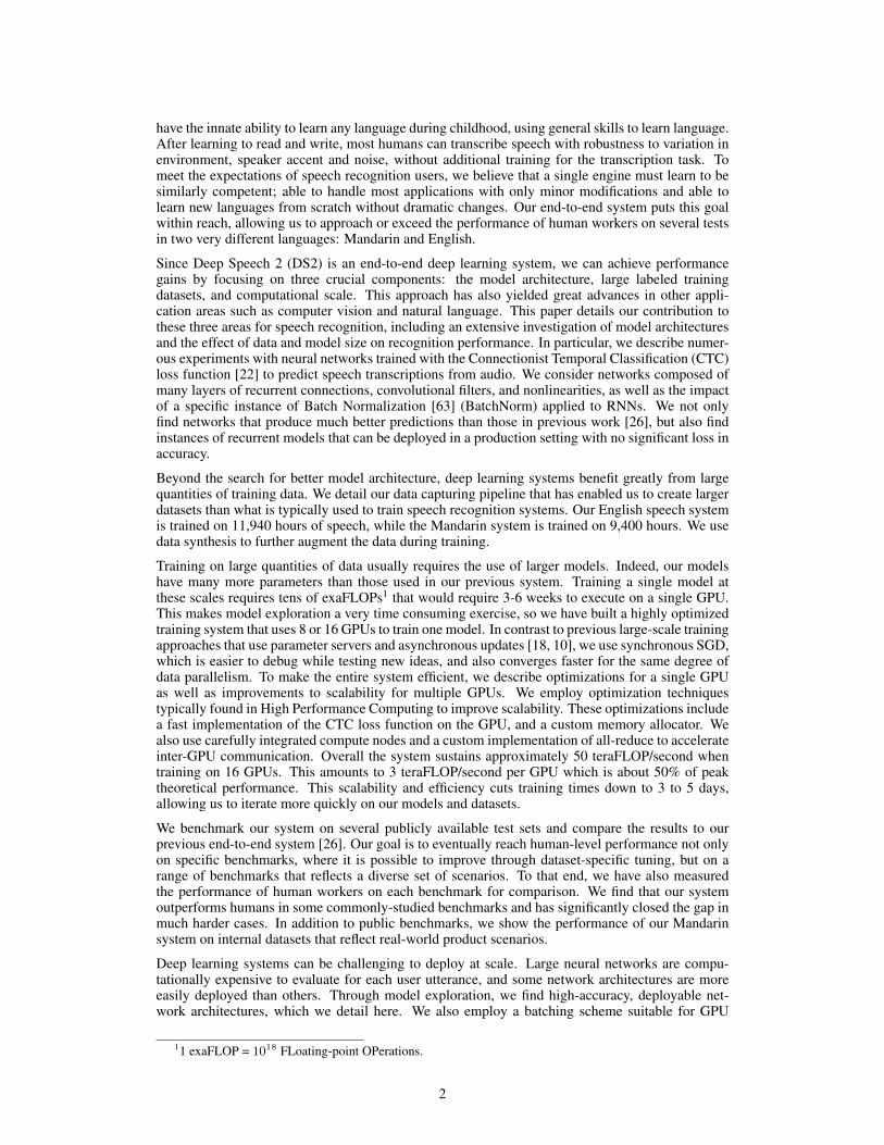


![[Harvard CS264] 14 - Dynamic Compilation for Massively Parallel Processors (Gregory Diamos, Georgia Tech)](https://static.documents.pub/doc/80x56/547bc106b4af9fd3158b4f84/harvard-cs264-14-dynamic-compilation-for-massively-parallel-processors-gregory-diamos-georgia-tech.jpg)


