The configuration space of a robotic arm in a tunnel. Federico Ardila * Hanner Bastidas † Cesar Ceballos ‡ John Guo § Abstract We study the motion of a robotic arm inside a rectangular tunnel. We prove that the configuration space of all possible positions of the robot is a CAT(0) cubical complex. This allows us to use techniques from geometric group theory to find the optimal way of moving the arm from one position to another. We also compute the diameter of the configuration space, that is, the longest distance between two positions of the robot. 1 Introduction We consider a robotic arm R m,n of length n moving in a rectangular tunnel of width m without self-intersecting. The robot consists of n links of unit length, attached sequentially, and facing up, down, or right. The base is affixed to the lower left corner. Figure 1 illustrates a possible position of the arm of length 8 in a tunnel of width 2. Figure 1: The robotic arm R 8,2 . The robotic arm may move freely using two kinds of local moves: • Switch corners: Two consecutive links facing different directions interchange directions. • Flip the end: The last link of the robot rotates 90 ◦ without intersecting itself. Figure 2: The two kinds of local moves of the robotic arm. We study the following fundamental problem. Problem 1.1. Move the robotic arm R m,n from one given position to another optimally. * San Francisco State University, San Francisco, USA; Univ. de Los Andes, Bogot´ a, Colombia; [email protected]. † Departamento de Matem´ aticas, Universidad del Valle, Cali, Colombia; [email protected]. ‡ Faculty of Mathematics, University of Vienna, Austria; [email protected]. § San Francisco State University, San Francisco, USA; [email protected]. This project is part of the SFSU-Colombia Combinatorics Initiative. FA was supported by the US NSF CAREER Award DMS-0956178 and NSF Combinatorics Award DMS-1600609. CC was supported by a Banting Postdoctoral Fellowship of the Canadian government, a York University research grant, and the Austrian FWF Grant F 5008-N15. 1 arXiv:1608.04800v1 [math.CO] 16 Aug 2016
Transcript
The configuration space of a robotic arm in a tunnel.
Federico Ardila∗ Hanner Bastidas† Cesar Ceballos‡ John Guo§
Abstract
We study the motion of a robotic arm inside a rectangular tunnel. We prove that theconfiguration space of all possible positions of the robot is a CAT(0) cubical complex.This allows us to use techniques from geometric group theory to find the optimal wayof moving the arm from one position to another. We also compute the diameter of theconfiguration space, that is, the longest distance between two positions of the robot.
1 Introduction
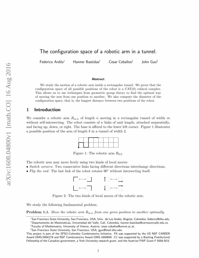
We consider a robotic arm Rm,n of length n moving in a rectangular tunnel of width mwithout self-intersecting. The robot consists of n links of unit length, attached sequentially,and facing up, down, or right. The base is affixed to the lower left corner. Figure 1 illustratesa possible position of the arm of length 8 in a tunnel of width 2.
Figure 1: The robotic arm R8,2.
The robotic arm may move freely using two kinds of local moves:• Switch corners: Two consecutive links facing different directions interchange directions.• Flip the end: The last link of the robot rotates 90◦ without intersecting itself.
Figure 2: The two kinds of local moves of the robotic arm.
We study the following fundamental problem.
Problem 1.1. Move the robotic arm Rm,n from one given position to another optimally.
∗San Francisco State University, San Francisco, USA; Univ. de Los Andes, Bogota, Colombia; [email protected].†Departamento de Matematicas, Universidad del Valle, Cali, Colombia; [email protected].‡Faculty of Mathematics, University of Vienna, Austria; [email protected].§San Francisco State University, San Francisco, USA; [email protected].
This project is part of the SFSU-Colombia Combinatorics Initiative. FA was supported by the US NSF CAREERAward DMS-0956178 and NSF Combinatorics Award DMS-1600609. CC was supported by a Banting PostdoctoralFellowship of the Canadian government, a York University research grant, and the Austrian FWF Grant F 5008-N15.
1
arX
iv:1
608.
0480
0v1
[m
ath.
CO
] 1
6 A
ug 2
016
When we are in a city we do not know well and we are trying to get from one locationto another, we will usually consult a map of the city to plan our route. This is a simplebut powerful idea. Our strategy to approach Problem 1.1 is pervasive in many branches ofmathematics: we will be to build and understand the “map” of all possible positions of therobot; we call it the configuration space Sm,n. Such spaces are also called state complexes,moduli spaces, or parameter spaces in other fields. Following work of Abrams–Ghrist [1] inapplied topology and Reeves [11] in geometric group theory, Ardila, Owen, and Sullivant [5]and Ardila, Baker, and Yatchak [3] showed how to solve Problem 1.1 for robots whose config-uration space is CAT(0); this is a notion of non-positive curvature defined in Section 4. Thisis the motivation for our main result.
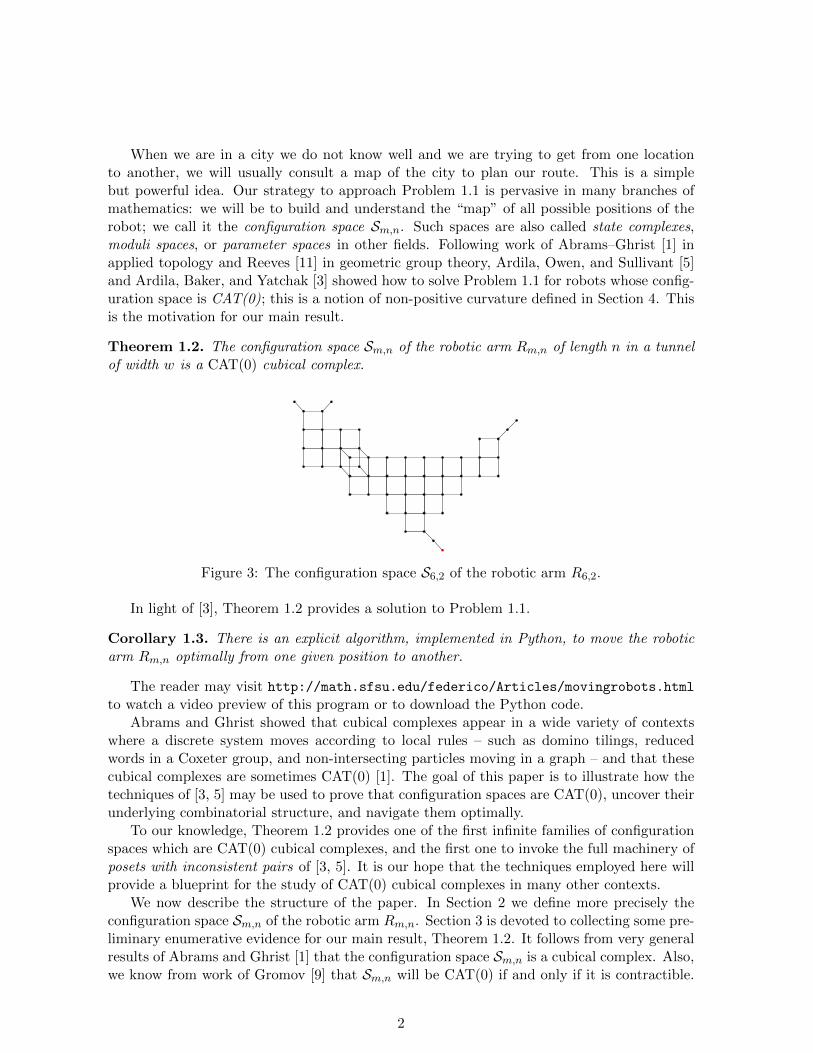
Theorem 1.2. The configuration space Sm,n of the robotic arm Rm,n of length n in a tunnelof width w is a CAT(0) cubical complex.
Figure 3: The configuration space S6,2 of the robotic arm R6,2.
In light of [3], Theorem 1.2 provides a solution to Problem 1.1.
Corollary 1.3. There is an explicit algorithm, implemented in Python, to move the roboticarm Rm,n optimally from one given position to another.
The reader may visit http://math.sfsu.edu/federico/Articles/movingrobots.htmlto watch a video preview of this program or to download the Python code.
Abrams and Ghrist showed that cubical complexes appear in a wide variety of contextswhere a discrete system moves according to local rules – such as domino tilings, reducedwords in a Coxeter group, and non-intersecting particles moving in a graph – and that thesecubical complexes are sometimes CAT(0) [1]. The goal of this paper is to illustrate how thetechniques of [3, 5] may be used to prove that configuration spaces are CAT(0), uncover theirunderlying combinatorial structure, and navigate them optimally.
To our knowledge, Theorem 1.2 provides one of the first infinite families of configurationspaces which are CAT(0) cubical complexes, and the first one to invoke the full machinery ofposets with inconsistent pairs of [3, 5]. It is our hope that the techniques employed here willprovide a blueprint for the study of CAT(0) cubical complexes in many other contexts.
We now describe the structure of the paper. In Section 2 we define more precisely theconfiguration space Sm,n of the robotic arm Rm,n. Section 3 is devoted to collecting some pre-liminary enumerative evidence for our main result, Theorem 1.2. It follows from very generalresults of Abrams and Ghrist [1] that the configuration space Sm,n is a cubical complex. Also,we know from work of Gromov [9] that Sm,n will be CAT(0) if and only if it is contractible.
Before launching into the proof that Sm,n is CAT(0), we first verify in the special case m = 2that this space has the correct Euler characteristic, equal to 1. We do it as follows.
Theorem 1.4. If cn,d denotes the number of d-dimensional cubes in the configuration spaceS2,n for a robot of width 2, then∑
The Euler characteristic of S2,n is χ(S2,n) = cn,0 − cn,1 + · · · . Substituting y = −1 abovewe find, in an expected but satisfying miracle of cancellation, that the generating functionfor χ(S2,n) is 1/(1− x) = 1 + x+ x2 + · · · .We obtain:
Theorem 1.5. The Euler characteristic of the configuration space S2,n equals 1.
In Section 4 we collect the tools we use to prove Theorem 1.2. Ardila, Owen, and Sul-livant [5] gave a bijection between CAT(0) cubical complexes X and combinatorial objectsP (X) called posets with inconsistent pairs or PIPs. The PIP P (X) is usually much simpler,and serves as a “remote control” to navigate the space X. This bijection allows us to provethat a (rooted) cubical complex is CAT(0) by identifying its corresponding PIP.1
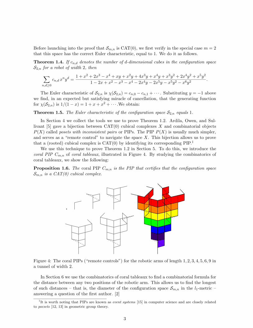
We use this technique to prove Theorem 1.2 in Section 5. To do this, we introduce thecoral PIP Cm,n of coral tableaux, illustrated in Figure 4. By studying the combinatorics ofcoral tableaux, we show the following:
Proposition 1.6. The coral PIP Cm,n is the PIP that certifies that the configuration spaceSm,n is a CAT(0) cubical complex.
Figure 4: The coral PIPs (“remote controls”) for the robotic arms of length 1, 2, 3, 4, 5, 6, 9 ina tunnel of width 2.
In Section 6 we use the combinatorics of coral tableaux to find a combinatorial formula forthe distance between any two positions of the robotic arm. This allows us to find the longestof such distances – that is, the diameter of the configuration space Sm,n in the l1-metric –answering a question of the first author. [2]
1It is worth noting that PIPs are known as event systems [15] in computer science and are closely relatedto pocsets [12, 13] in geometric group theory.
3
Theorem 1.7. The diameter of the transition graph of the robot Rm,n of length n in a tunnelof width m ≥ 2 is
diamG(Rm,n) =
{d(Lm,n, Hm,n) for n < 6d(Lm,n, L
+m,n) for n ≥ 6,
where Lm,n = umrdmrumr . . . is the left justified position, L+m,n = (urdr)Lm,n−4 and Hm,n
is the fully horizontal position (see Figure 19). A precise formula is stated in Theorem 6.4.
Finally, in Section 7 we discuss our solution to Problem 1.1. As explained in [3], we use thecoral PIP as a remote control for our robotic arm. This allows us to implement an algorithmto move the robotic arm Rm,n optimally from one position to another.
2 The configuration space
Recall that Rm,n is a robotic arm consisting of n links of unit length attached sequentally,and facing up, down, or right. The robot is inside a rectangular tunnel of width m andpinned down at the bottom left corner of the tunnel. It moves inside the tunnel withoutself-intersecting, by switching corners and flipping the end as illustrated in Figure 2.
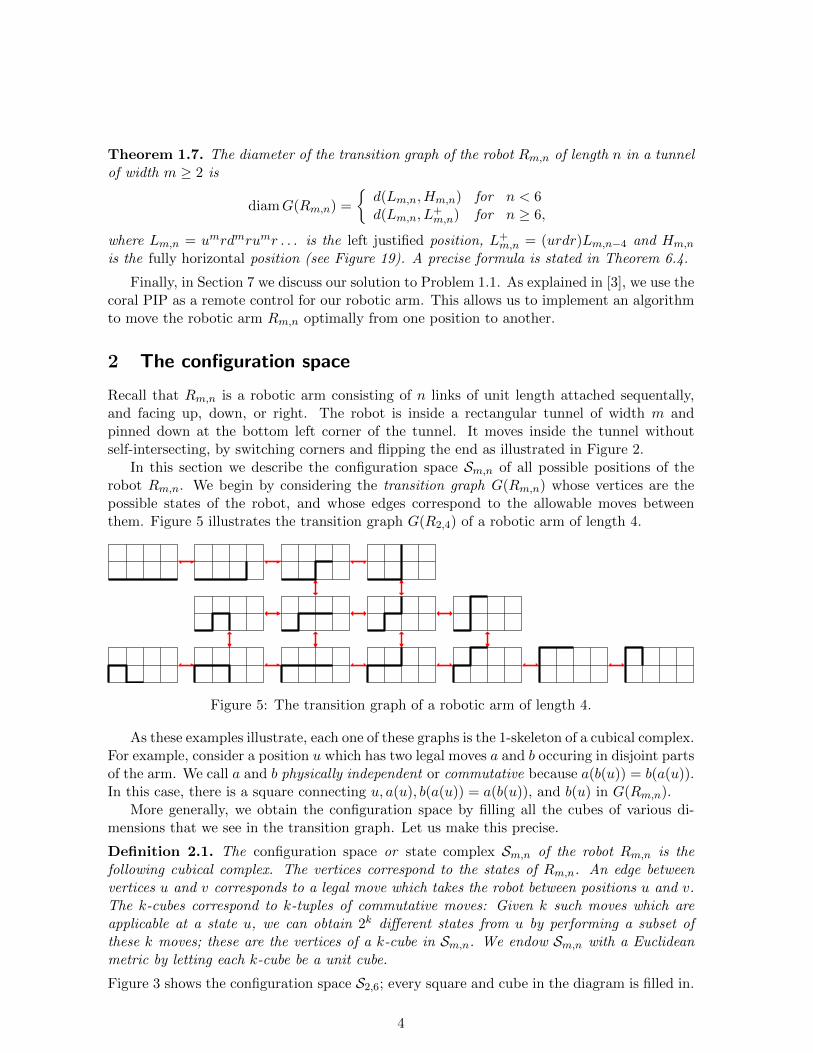
In this section we describe the configuration space Sm,n of all possible positions of therobot Rm,n. We begin by considering the transition graph G(Rm,n) whose vertices are thepossible states of the robot, and whose edges correspond to the allowable moves betweenthem. Figure 5 illustrates the transition graph G(R2,4) of a robotic arm of length 4.
Figure 5: The transition graph of a robotic arm of length 4.
As these examples illustrate, each one of these graphs is the 1-skeleton of a cubical complex.For example, consider a position u which has two legal moves a and b occuring in disjoint partsof the arm. We call a and b physically independent or commutative because a(b(u)) = b(a(u)).In this case, there is a square connecting u, a(u), b(a(u)) = a(b(u)), and b(u) in G(Rm,n).
More generally, we obtain the configuration space by filling all the cubes of various di-mensions that we see in the transition graph. Let us make this precise.
Definition 2.1. The configuration space or state complex Sm,n of the robot Rm,n is thefollowing cubical complex. The vertices correspond to the states of Rm,n. An edge betweenvertices u and v corresponds to a legal move which takes the robot between positions u and v.The k-cubes correspond to k-tuples of commutative moves: Given k such moves which areapplicable at a state u, we can obtain 2k different states from u by performing a subset ofthese k moves; these are the vertices of a k-cube in Sm,n. We endow Sm,n with a Euclideanmetric by letting each k-cube be a unit cube.
Figure 3 shows the configuration space S2,6; every square and cube in the diagram is filled in.
4
3 Face enumeration and the Euler characteristic of S2,n
The main structural result of this paper, Theorem 1.2, is that the configuration space Sm,nof our robot is a CAT(0) cubical complex. This is a subtle metric property defined in Section4 and proved in Section 5. As a prelude, this section is devoted to proving a partial result inthat direction. It is known [7, 9] that CAT(0) spaces are contractible, and hence have Eulercharacteristic equal to 1. We now prove:
Theorem 1.5. The Euler characteristic of the configuration space S2,n equals 1.
This provides enumerative evidence for our main result in width m = 2. While we were stuckfor several weeks trying to prove Theorem 1.2, we found this evidence very encouraging.
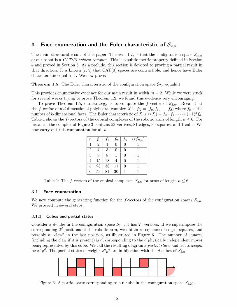
To prove Theorem 1.5, our strategy is to compute the f -vector of S2,n. Recall thatthe f -vector of a d-dimensional polyhedral complex X is fX = (f0, f1, . . . , fd) where fk is thenumber of k-dimensional faces. The Euler characteristic of X is χ(X) = f0−f1+· · ·+(−1)dfd.Table 1 shows the f -vectors of the cubical complexes of the robotic arms of length n ≤ 6. Forinstance, the complex of Figure 3 contains 53 vertices, 81 edges, 30 squares, and 1 cube. Wenow carry out this computation for all n.
n f0 f1 f2 f3 χ(S2,n)
1 2 1 0 0 1
2 4 3 0 0 1
3 8 8 1 0 1
4 15 18 4 0 1
5 28 38 11 0 1
6 53 81 30 1 1
Table 1: The f -vectors of the cubical complexes S2,n for arms of length n ≤ 6.
3.1 Face enumeration
We now compute the generating function for the f -vectors of the configuration spaces S2,n.We proceed in several steps.
3.1.1 Cubes and partial states
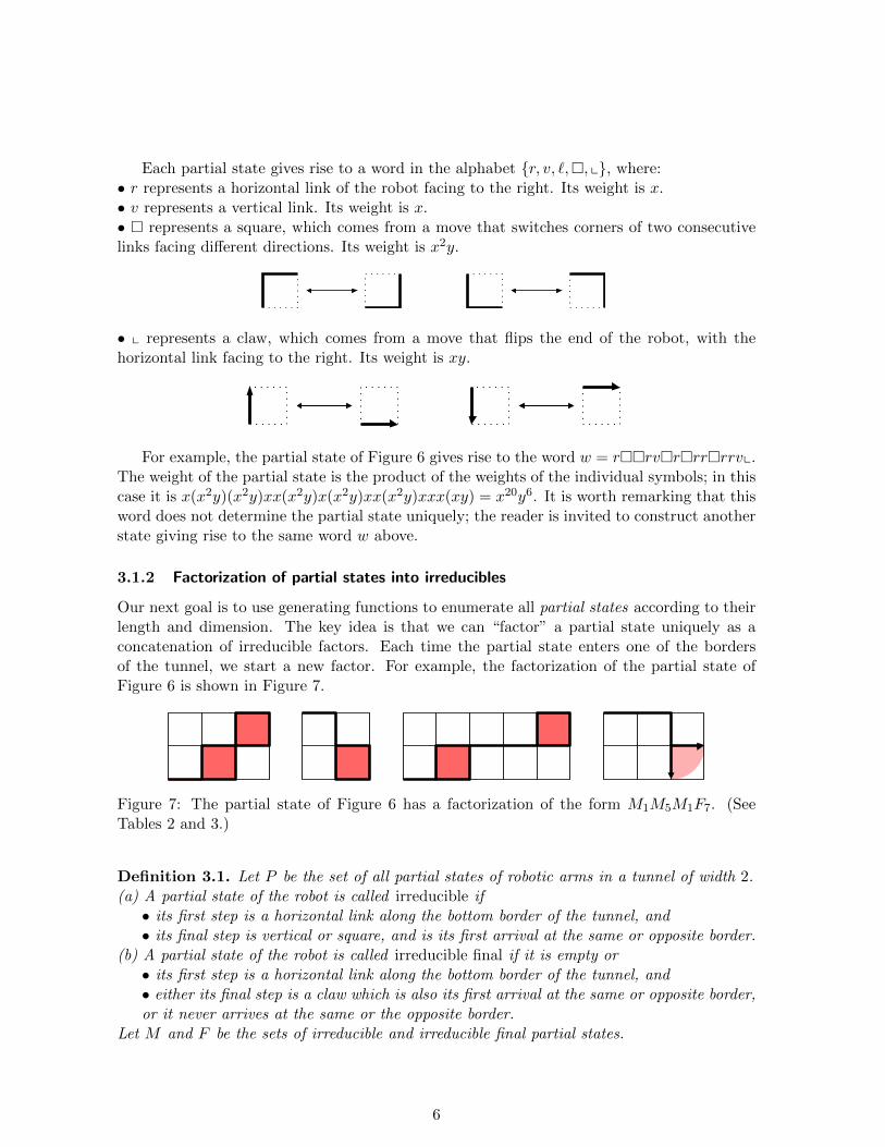
Consider a d-cube in the configuration space S2,n; it has 2d vertices. If we superimpose thecorresponding 2d positions of the robotic arm, we obtain a sequence of edges, squares, andpossibly a “claw” in the last position, as illustrated in Figure 6. The number of squares(including the claw if it is present) is d, corresponding to the d physically independent movesbeing represented by this cube. We call the resulting diagram a partial state, and let its weightbe xnyd. The partial states of weight xnyd are in bijection with the d-cubes of S2,n.
Figure 6: A partial state corresponding to a 6-cube in the configuration space S2,20.
5
Each partial state gives rise to a word in the alphabet {r, v, `,�, x}, where:• r represents a horizontal link of the robot facing to the right. Its weight is x.• v represents a vertical link. Its weight is x.• � represents a square, which comes from a move that switches corners of two consecutivelinks facing different directions. Its weight is x2y.
• x represents a claw, which comes from a move that flips the end of the robot, with thehorizontal link facing to the right. Its weight is xy.
For example, the partial state of Figure 6 gives rise to the word w = r��rv�r�rr�rrvx.The weight of the partial state is the product of the weights of the individual symbols; in thiscase it is x(x2y)(x2y)xx(x2y)x(x2y)xx(x2y)xxx(xy) = x20y6. It is worth remarking that thisword does not determine the partial state uniquely; the reader is invited to construct anotherstate giving rise to the same word w above.
3.1.2 Factorization of partial states into irreducibles
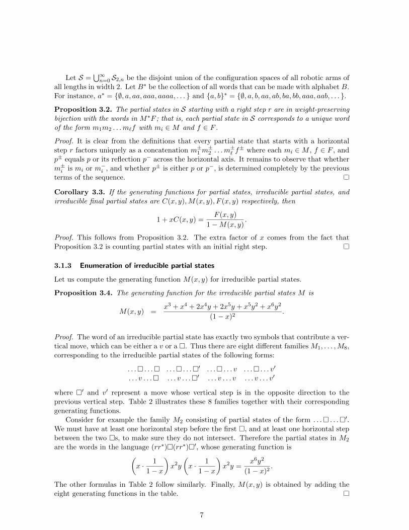
Our next goal is to use generating functions to enumerate all partial states according to theirlength and dimension. The key idea is that we can “factor” a partial state uniquely as aconcatenation of irreducible factors. Each time the partial state enters one of the bordersof the tunnel, we start a new factor. For example, the factorization of the partial state ofFigure 6 is shown in Figure 7.
Figure 7: The partial state of Figure 6 has a factorization of the form M1M5M1F7. (SeeTables 2 and 3.)
Definition 3.1. Let P be the set of all partial states of robotic arms in a tunnel of width 2.(a) A partial state of the robot is called irreducible if• its first step is a horizontal link along the bottom border of the tunnel, and• its final step is vertical or square, and is its first arrival at the same or opposite border.
(b) A partial state of the robot is called irreducible final if it is empty or• its first step is a horizontal link along the bottom border of the tunnel, and• either its final step is a claw which is also its first arrival at the same or opposite border,or it never arrives at the same or the opposite border.
Let M and F be the sets of irreducible and irreducible final partial states.
6
Let S =⋃∞n=0 S2,n be the disjoint union of the configuration spaces of all robotic arms of
all lengths in width 2. Let B∗ be the collection of all words that can be made with alphabet B.For instance, a∗ = {∅, a, aa, aaa, aaaa, . . . } and {a, b}∗ = {∅, a, b, aa, ab, ba, bb, aaa, aab, . . . }.Proposition 3.2. The partial states in S starting with a right step r are in weight-preservingbijection with the words in M∗F ; that is, each partial state in S corresponds to a unique wordof the form m1m2 . . .m`f with mi ∈M and f ∈ F .
Proof. It is clear from the definitions that every partial state that starts with a horizontalstep r factors uniquely as a concatenation m±1 m
±2 . . .m
±` f± where each mi ∈M , f ∈ F , and
p± equals p or its reflection p− across the horizontal axis. It remains to observe that whetherm±i is mi or m−i , and whether p± is either p or p−, is determined completely by the previousterms of the sequence.
Corollary 3.3. If the generating functions for partial states, irreducible partial states, andirreducible final partial states are C(x, y),M(x, y), F (x, y) respectively, then
1 + xC(x, y) =F (x, y)
1−M(x, y).
Proof. This follows from Proposition 3.2. The extra factor of x comes from the fact thatProposition 3.2 is counting partial states with an initial right step.
3.1.3 Enumeration of irreducible partial states
Let us compute the generating function M(x, y) for irreducible partial states.
Proposition 3.4. The generating function for the irreducible partial states M is
M(x, y) =x3 + x4 + 2x4y + 2x5y + x5y2 + x6y2
(1− x)2.
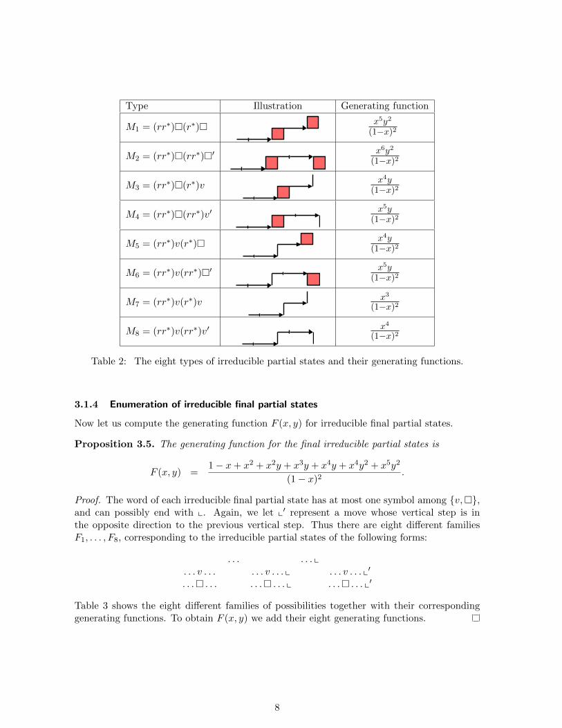
Proof. The word of an irreducible partial state has exactly two symbols that contribute a ver-tical move, which can be either a v or a �. Thus there are eight different families M1, . . . ,M8,corresponding to the irreducible partial states of the following forms:
. . . v . . .� . . . v . . .�′ . . . v . . . v . . . v . . . v′
where �′ and v′ represent a move whose vertical step is in the opposite direction to theprevious vertical step. Table 2 illustrates these 8 families together with their correspondinggenerating functions.
Consider for example the family M2 consisting of partial states of the form . . .� . . .�′.We must have at least one horizontal step before the first �, and at least one horizontal stepbetween the two �s, to make sure they do not intersect. Therefore the partial states in M2
are the words in the language (rr∗)�(rr∗)�′, whose generating function is(x · 1
1− x
)x2y
(x · 1
1− x
)x2y =
x6y2
(1− x)2.
The other formulas in Table 2 follow similarly. Finally, M(x, y) is obtained by adding theeight generating functions in the table.
7
Type Illustration Generating function
M1 = (rr∗)�(r∗)�x5y2
(1−x)2
M2 = (rr∗)�(rr∗)�′x6y2
(1−x)2
M3 = (rr∗)�(r∗)vx4y
(1−x)2
M4 = (rr∗)�(rr∗)v′x5y
(1−x)2
M5 = (rr∗)v(r∗)�x4y
(1−x)2
M6 = (rr∗)v(rr∗)�′x5y
(1−x)2
M7 = (rr∗)v(r∗)vx3
(1−x)2
M8 = (rr∗)v(rr∗)v′x4
(1−x)2
Table 2: The eight types of irreducible partial states and their generating functions.
3.1.4 Enumeration of irreducible final partial states
Now let us compute the generating function F (x, y) for irreducible final partial states.
Proposition 3.5. The generating function for the final irreducible partial states is
Proof. The word of each irreducible final partial state has at most one symbol among {v,�},and can possibly end with x. Again, we let x′ represent a move whose vertical step is inthe opposite direction to the previous vertical step. Thus there are eight different familiesF1, . . . , F8, corresponding to the irreducible partial states of the following forms:
. . . . . . x. . . v . . . . . . v . . . x . . . v . . . x′
. . .� . . . . . .� . . . x . . .� . . . x′
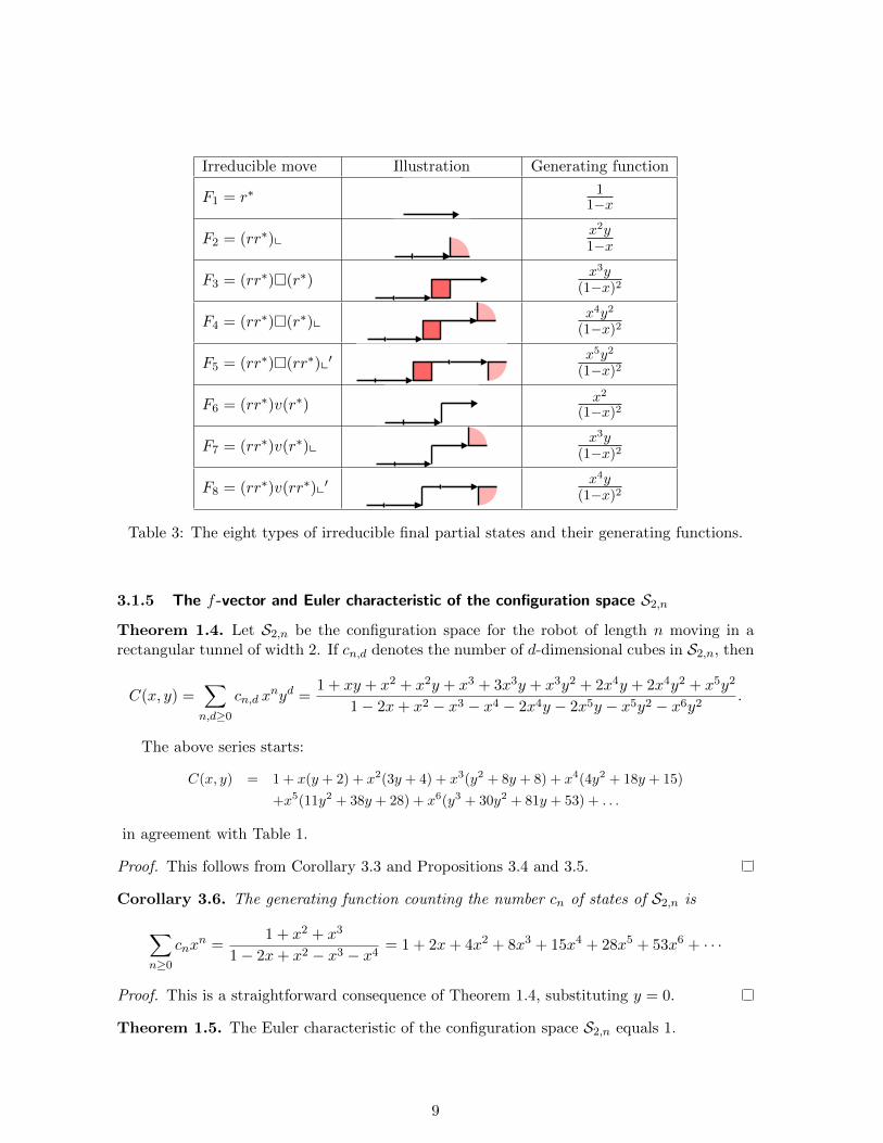
Table 3 shows the eight different families of possibilities together with their correspondinggenerating functions. To obtain F (x, y) we add their eight generating functions.
8
Irreducible move Illustration Generating function
F1 = r∗1
1−x
F2 = (rr∗)xx2y1−x
F3 = (rr∗)�(r∗)x3y
(1−x)2
F4 = (rr∗)�(r∗)xx4y2
(1−x)2
F5 = (rr∗)�(rr∗)x′x5y2
(1−x)2
F6 = (rr∗)v(r∗)x2
(1−x)2
F7 = (rr∗)v(r∗)xx3y
(1−x)2
F8 = (rr∗)v(rr∗)x′x4y
(1−x)2
Table 3: The eight types of irreducible final partial states and their generating functions.
3.1.5 The f-vector and Euler characteristic of the configuration space S2,nTheorem 1.4. Let S2,n be the configuration space for the robot of length n moving in arectangular tunnel of width 2. If cn,d denotes the number of d-dimensional cubes in S2,n, then
Proof. This is a straightforward consequence of Theorem 1.4, substituting y = 0.
Theorem 1.5. The Euler characteristic of the configuration space S2,n equals 1.
9
Proof. The generating function for the Euler characteristic of S2,n is
∑n≥0
χ(S2,n)xn =∑n≥0
∑d≥0
(−1)dcn,d
xn = C(x,−1)
=1− x− x3 + x5
1− 2x+ x2 − x3 + x4 + x5 − x6
=1
1− x = 1 + x+ x2 + x3 + . . .
by Theorem 1.4. All the coefficients of this series are equal to 1, as desired.
4 The combinatorics of CAT(0) cube complexes
4.1 CAT(0) spaces
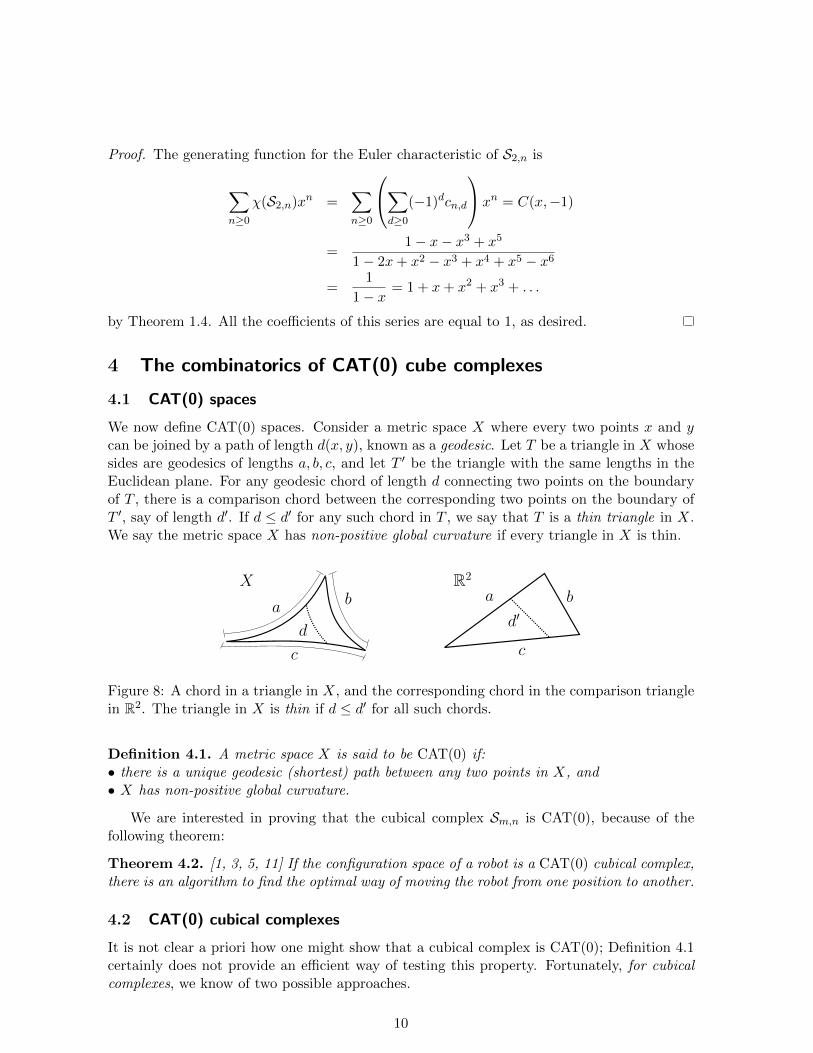
We now define CAT(0) spaces. Consider a metric space X where every two points x and ycan be joined by a path of length d(x, y), known as a geodesic. Let T be a triangle in X whosesides are geodesics of lengths a, b, c, and let T ′ be the triangle with the same lengths in theEuclidean plane. For any geodesic chord of length d connecting two points on the boundaryof T , there is a comparison chord between the corresponding two points on the boundary ofT ′, say of length d′. If d ≤ d′ for any such chord in T , we say that T is a thin triangle in X.We say the metric space X has non-positive global curvature if every triangle in X is thin.
4.2. The link condition. There is a well-known combinatorial approach to deter-mining when a cubical complex is nonpositively curved due to Gromov.
Definition 4.3. Let X denote a cell complex and let v denote a vertex of X . The linkof v, !k[v], is defined to be the abstract simplicial complex whose k-dimensionalsimplices are the (k + 1)-dimensional cells incident to v with the natural boundaryrelationships.
Certain global topological features of a metric cubical complex are completely de-termined by the local structure of the vertex links: a theorem of Gromov [26] assertsthat a finite dimensional Euclidean cubical complex is NPC if and only if the linkof every vertex is a flag complex without digons. Recall: a digon is a pair of ver-tices connected by two edges, and a flag complex is a simplicial complex whichis maximal among all simplicial complexes with the same 1-dimensional skeleton.Gromov’s theorem permits us an elementary proof of the following general result.
Theorem 4.4. The state complex of any locally finite reconfigurable system is NPC.
PROOF: Gromov’s theorem is stated for finite dimensional Euclidean cubical com-plexes with unit length cubes. It holds, however, for non-unit length cubes whenthere are a finite number of isometry classes of cubes (the finite shapes condition) [6].Locally finite reconfigurable systems possess locally finite and finite dimensionalstate complexes, which automatically satisfy the finite shapes condition (locally).
Let u denote a vertex of S. Consider the link !k[u]. The 0-cells of the !k[u] corre-spond to all edges in S(1) incident to u; that is, actions of generators based at u. Ak-cell of !k[u] is thus a commuting set of k + 1 of these generators based at u.
We argue first that there are no digons in !k[u] for any u " S. Assume that "1 and "2
are admissible generators for the state u, and that these two generators correspondto the vertices of a digon in !k[u]. Each edge of the digon in !k[u] corresponds toa distinct 2-cell in S having a corner at u and edges at u corresponding to "1 and"2. By Definition 2.7, each such 2-cell is the equivalence class [u; ("1, "2)]: the two2-cells are therefore equivalent and not distinct.
To complete the proof, we must show that the link is a flag complex. The interpre-tation of the flag condition for a state complex is as follows: if at u " S, one hasa set of k generators "!i , of which each pair of generators commutes, then the full
Figure 8: A chord in a triangle in X, and the corresponding chord in the comparison trianglein R2. The triangle in X is thin if d ≤ d′ for all such chords.
Definition 4.1. A metric space X is said to be CAT(0) if:• there is a unique geodesic (shortest) path between any two points in X, and• X has non-positive global curvature.
We are interested in proving that the cubical complex Sm,n is CAT(0), because of thefollowing theorem:
Theorem 4.2. [1, 3, 5, 11] If the configuration space of a robot is a CAT(0) cubical complex,there is an algorithm to find the optimal way of moving the robot from one position to another.
4.2 CAT(0) cubical complexes
It is not clear a priori how one might show that a cubical complex is CAT(0); Definition 4.1certainly does not provide an efficient way of testing this property. Fortunately, for cubicalcomplexes, we know of two possible approaches.
10
The topological approach. The first approach uses Gromov’s groundbreaking result thatthis subtle metric property has a topological–combinatorial characterization:
Theorem 4.3. [9] A cubical complex is CAT(0) if and only if it is simply connected, and thelink of every vertex is a flag simplicial complex.
Recall that a simplicial complex ∆ is flag if it has no empty simplices; more explicitly, ifthe 1-skeleton of a simplex is in ∆, then that simplex must be in ∆. It is easy to see that,in the configuration space of a robot, every vertex has a flag link. Therefore, one approachto prove that these spaces are CAT(0) is to prove they are simply connected; see [1, 8] forexamples of this approach.
The combinatorial approach. We will use a purely combinatorial characterization of finiteCAT(0) cube complexes [5, 12, 13, 15]; we use the formulation of Ardila, Owen, and Sulli-vant [5]. After drawing enough CAT(0) cube complexes, one might notice that they look alot like distributive lattices. In trying to make this statement precise, one discovers a gener-alization of Birkhoff’s Fundamental Theorem of Distributive Lattices; there are bijections:
distributive lattices ←→ posets
rooted CAT(0) cubical complexes ←→ posets with inconsistent pairs (PIPs)
Hence to prove that a cubical complex is a CAT(0) cubical complex, it suffices to choosea root for it, and identify the corresponding PIP. By the above correspondence, this PIP willserve as a “certificate” that the complex is CAT(0). For a reasonably small complex, it isstraighforward to identify the PIP, as described below. For an infinite family of configurationspaces like the one that interests us, one may do this for a few small examples and hopeto identify a pattern that one can prove in general. Along the way, one gains a betterunderstanding of the combinatorial structure of the complexes one is studying. This approachwas first carried out in [3] for two examples, and the goal of this paper is to carry it out for therobots Rm,n. This family is considerably more complicated than the ones in [3], in particular,because it appears to be the first known example where the skeleton of the complex is not adistributive lattice, and the PIP does indeed have inconsistent pairs.
1
2
4
65
3v
1
2 4
6
3
5 12345
12
123
124
234 1246
24
1234
2
2
123
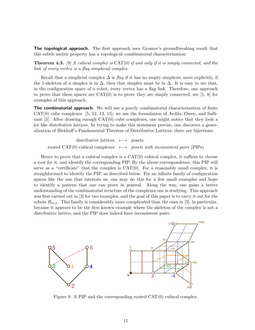
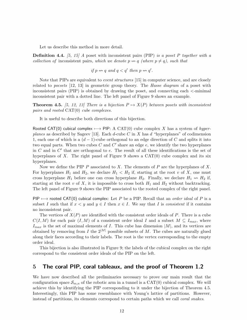
Figure 9: A PIP and the corresponding rooted CAT(0) cubical complex.
11
Let us describe this method in more detail.
Definition 4.4. [5, 15] A poset with inconsistent pairs (PIP) is a poset P together with acollection of inconsistent pairs, which we denote p= q (where p 6= q), such that
if p= q and q < q′ then p= q′.
Note that PIPs are equivalent to event structures [15] in computer science, and are closelyrelated to pocsets [12, 13] in geometric group theory. The Hasse diagram of a poset withinconsistent pairs (PIP) is obtained by drawing the poset, and connecting each <-minimalinconsistent pair with a dotted line. The left panel of Figure 9 shows an example.
Theorem 4.5. [5, 12, 13] There is a bijection P 7→ X(P ) between posets with inconsistentpairs and rooted CAT(0) cube complexes.
It is useful to describe both directions of this bijection.
Rooted CAT(0) cubical complex 7−→ PIP: A CAT(0) cube complex X has a system of hyper-planes as described by Sageev [13]. Each d-cube C in X has d “hyperplanes” of codimension1, each one of which is a (d− 1)-cube orthogonal to an edge direction of C and splits it intotwo equal parts. When two cubes C and C ′ share an edge e, we identify the two hyperplanesin C and in C ′ that are orthogonal to e. The result of all these identifications is the set ofhyperplanes of X. The right panel of Figure 9 shows a CAT(0) cube complex and its sixhyperplanes.
Now we define the PIP P associated to X. The elements of P are the hyperplanes of X.For hyperplanes H1 and H2, we declare H1 < H2 if, starting at the root v of X, one mustcross hyperplane H1 before one can cross hyperplane H2. Finally, we declare H1 = H2 if,starting at the root v of X, it is impossible to cross both H1 and H2 without backtracking.The left panel of Figure 9 shows the PIP associated to the rooted complex of the right panel.
PIP 7−→ rooted CAT(0) cubical complex: Let P be a PIP. Recall that an order ideal of P is asubset I such that if x < y and y ∈ I then x ∈ I. We say that I is consistent if it containsno inconsistent pair.
The vertices of X(P ) are identified with the consistent order ideals of P . There is a cubeC(I,M) for each pair (I,M) of a consistent order ideal I and a subset M ⊆ Imax, whereImax is the set of maximal elements of I. This cube has dimension |M |, and its vertices areobtained by removing from I the 2|M | possible subsets of M . The cubes are naturally gluedalong their faces according to their labels. The root is the vertex corresponding to the emptyorder ideal.
This bijection is also illustrated in Figure 9; the labels of the cubical complex on the rightcorrespond to the consistent order ideals of the PIP on the left.
5 The coral PIP, coral tableaux, and the proof of Theorem 1.2
We have now described all the preliminaries necessary to prove our main result that theconfiguration space Sm,n of the robotic arm in a tunnel is a CAT(0) cubical complex. We willachieve this by identifying the PIP corresponding to it under the bijection of Theorem 4.5.Interestingly, this PIP has some resemblance with Young’s lattice of partitions. However,instead of partitions, its elements correspond to certain paths which we call coral snakes.
12
5.1 The coral PIP
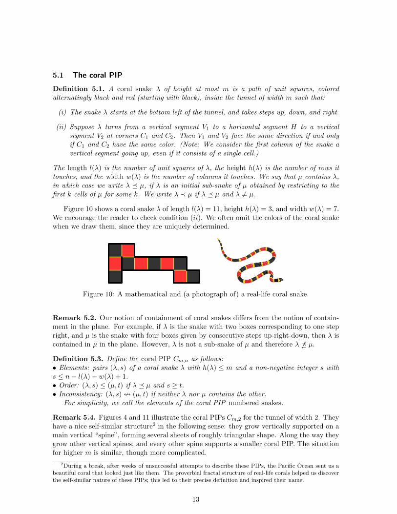
Definition 5.1. A coral snake λ of height at most m is a path of unit squares, coloredalternatingly black and red (starting with black), inside the tunnel of width m such that:
(i) The snake λ starts at the bottom left of the tunnel, and takes steps up, down, and right.
(ii) Suppose λ turns from a vertical segment V1 to a horizontal segment H to a verticalsegment V2 at corners C1 and C2. Then V1 and V2 face the same direction if and onlyif C1 and C2 have the same color. (Note: We consider the first column of the snake avertical segment going up, even if it consists of a single cell.)
The length l(λ) is the number of unit squares of λ, the height h(λ) is the number of rows ittouches, and the width w(λ) is the number of columns it touches. We say that µ contains λ,in which case we write λ � µ, if λ is an initial sub-snake of µ obtained by restricting to thefirst k cells of µ for some k. We write λ ≺ µ if λ � µ and λ 6= µ.
Figure 10 shows a coral snake λ of length l(λ) = 11, height h(λ) = 3, and width w(λ) = 7.We encourage the reader to check condition (ii). We often omit the colors of the coral snakewhen we draw them, since they are uniquely determined.
Figure 10: A mathematical and (a photograph of) a real-life coral snake.
Remark 5.2. Our notion of containment of coral snakes differs from the notion of contain-ment in the plane. For example, if λ is the snake with two boxes corresponding to one stepright, and µ is the snake with four boxes given by consecutive steps up-right-down, then λ iscontained in µ in the plane. However, λ is not a sub-snake of µ and therefore λ � µ.
Definition 5.3. Define the coral PIP Cm,n as follows:• Elements: pairs (λ, s) of a coral snake λ with h(λ) ≤ m and a non-negative integer s withs ≤ n− l(λ)− w(λ) + 1.• Order: (λ, s) ≤ (µ, t) if λ � µ and s ≥ t.• Inconsistency: (λ, s) = (µ, t) if neither λ nor µ contains the other.
For simplicity, we call the elements of the coral PIP numbered snakes.
Remark 5.4. Figures 4 and 11 illustrate the coral PIPs Cm,2 for the tunnel of width 2. Theyhave a nice self-similar structure2 in the following sense: they grow vertically supported on amain vertical “spine”, forming several sheets of roughly triangular shape. Along the way theygrow other vertical spines, and every other spine supports a smaller coral PIP. The situationfor higher m is similar, though more complicated.
2During a break, after weeks of unsuccessful attempts to describe these PIPs, the Pacific Ocean sent us abeautiful coral that looked just like them. The proverbial fractal structure of real-life corals helped us discoverthe self-similar nature of these PIPs; this led to their precise definition and inspired their name.
13
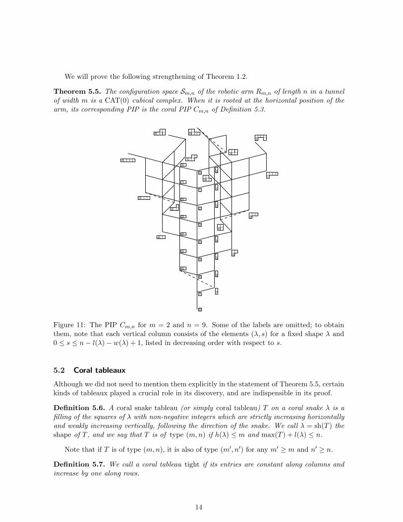
We will prove the following strengthening of Theorem 1.2.
Theorem 5.5. The configuration space Sm,n of the robotic arm Rm,n of length n in a tunnelof width m is a CAT(0) cubical complex. When it is rooted at the horizontal position of thearm, its corresponding PIP is the coral PIP Cm,n of Definition 5.3.
8
6
5
4
3
2
1
0
7 7
6
5
4
2
1
0
6
5
4
3
2
1
0
5
4
3
21
1
0
0
4
3
2
10
0
Figure 11: The PIP Cm,n for m = 2 and n = 9. Some of the labels are omitted; to obtainthem, note that each vertical column consists of the elements (λ, s) for a fixed shape λ and0 ≤ s ≤ n− l(λ)− w(λ) + 1, listed in decreasing order with respect to s.
5.2 Coral tableaux
Although we did not need to mention them explicitly in the statement of Theorem 5.5, certainkinds of tableaux played a crucial role in its discovery, and are indispensible in its proof.
Definition 5.6. A coral snake tableau (or simply coral tableau) T on a coral snake λ is afilling of the squares of λ with non-negative integers which are strictly increasing horizontallyand weakly increasing vertically, following the direction of the snake. We call λ = sh(T ) theshape of T , and we say that T is of type (m,n) if h(λ) ≤ m and max(T ) + l(λ) ≤ n.
Note that if T is of type (m,n), it is also of type (m′, n′) for any m′ ≥ m and n′ ≥ n.
Definition 5.7. We call a coral tableau tight if its entries are constant along columns andincrease by one along rows.
14
1
3
4 6
8
8 10
11 12
13 2
2
2 3
3 4 5 6 7
7 8
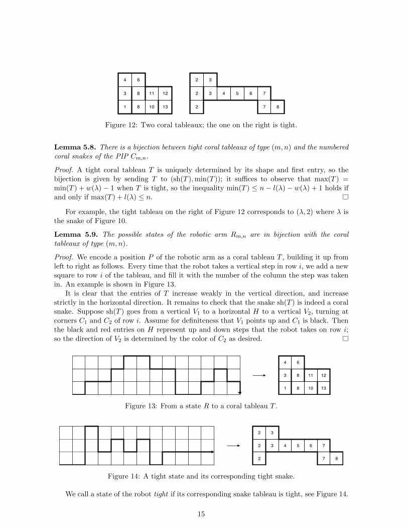
Figure 12: Two coral tableaux; the one on the right is tight.
Lemma 5.8. There is a bijection between tight coral tableaux of type (m,n) and the numberedcoral snakes of the PIP Cm,n.
Proof. A tight coral tableau T is uniquely determined by its shape and first entry, so thebijection is given by sending T to (sh(T ),min(T )); it suffices to observe that max(T ) =min(T ) + w(λ)− 1 when T is tight, so the inequality min(T ) ≤ n− l(λ)− w(λ) + 1 holds ifand only if max(T ) + l(λ) ≤ n.
For example, the tight tableau on the right of Figure 12 corresponds to (λ, 2) where λ isthe snake of Figure 10.
Lemma 5.9. The possible states of the robotic arm Rm,n are in bijection with the coraltableaux of type (m,n).
Proof. We encode a position P of the robotic arm as a coral tableau T , building it up fromleft to right as follows. Every time that the robot takes a vertical step in row i, we add a newsquare to row i of the tableau, and fill it with the number of the column the step was takenin. An example is shown in Figure 13.
It is clear that the entries of T increase weakly in the vertical direction, and increasestrictly in the horizontal direction. It remains to check that the snake sh(T ) is indeed a coralsnake. Suppose sh(T ) goes from a vertical V1 to a horizontal H to a vertical V2, turning atcorners C1 and C2 of row i. Assume for definiteness that V1 points up and C1 is black. Thenthe black and red entries on H represent up and down steps that the robot takes on row i;so the direction of V2 is determined by the color of C2 as desired.
1
3
4 6
8
8 10
11 12
13
Figure 13: From a state R to a coral tableau T .
2
2
2 3
3 4 5 6 7
7 8
Figure 14: A tight state and its corresponding tight snake.
We call a state of the robot tight if its corresponding snake tableau is tight, see Figure 14.
15
5.3 Proof of our main structural theorem
We are now ready to prove our strengthening of the main result of this paper, Theorem 1.2.
Theorem 5.5. The configuration space Sm,n of the robotic arm Rm,n of length n in a tunnelof width m is a CAT(0) cubical complex. When it is rooted at the horizontal position of thearm, its corresponding PIP is the coral PIP Cm,n of Definition 5.3.
Proof. We need to show that, when rooted at the horizontal position, Sm,n is the cubicalcomplex X(Cm,n) associated to the PIP Cm,n under the bijection of Theorem 4.5. We proceedin three steps.
Step 1. Decomposing Sm,n and Cm,n by shape.
For a coral snake λ of type (m,n) let Sλm,n be the induced subcomplex of Sm,n whose
vertices are the coral tableaux T with sh(T ) � λ. Similarly, let Cλm,n be the subPIP of Cm,nconsisting of the pairs (µ, s) such that µ � λ. Notice that Cλm,n is a poset which has noinconsistent pairs. We have
Sm,n =⋃
λ of type (m,n)
Sλm,n Cm,n =⋃
λ of type (m,n)
Cλm,n (1)
where each (non-disjoint) union is over the coral tableaux λ of type (m,n). (Of course, sinceλ � λ′ implies Sλm,n ⊆ Sλ
′m,n and Cλm,n ⊆ Cλ
′m,n, it is sufficient to take the union over those λ
which are maximal under inclusion.)
Step 2. Showing Sλm,n = X(Cλm,n) for each shape λ.
We begin by establishing a bijection between the sets of vertices of both complexes. Thevertices of X(Cλm,n) correspond to the consistent order ideals of the coral PIP Cλm,n. Since
Cλm,n has no inconsistent pairs, these are all the order ideals of Cλm,n, which are the elements
of the distributive lattice J(Cλm,n).
The vertices of Sλm,n correspond to the coral tableaux T of type (m,n) with shape sh(T ) �λ by Lemma 5.9. Let us extend each such tableau T to a tableau of shape λ by adding entriesequal to∞ on each cell of λ−sh(T ). We may then identify the set of vertices V (Sλm,n) with theresulting set of extended coral tableaux of shape λ whose finite entries x satisfy x+ l(λ) ≤ n.
This set V (Sλm,n) of extended λ-tableaux forms a poset under reverse componentwise order.
Note that if T1 and T2 are in V (Sλm,n) then the componentwise maximum T1 ∧ T2 and the
componentwise minimum T1 ∨ T2 are also in V (Sλm,n). Then the meet ∧ and join ∨ make
V (Sλm,n) into a lattice. In fact, the definitions of ∧ and ∨ imply that this lattice is distributive.
Birkhoff’s Fundamental Theorem of Distributive Lattices then implies that V (Sλm,n) ∼= J(P )
where P is the subposet of join-irreducible elements of V (Sλm,n). One easily verifies that P
consists precisely of the tight tableaux of type (m,n) and shape λ, so P ∼= Cλm,n. It followsthat the coral tableaux T of type (m,n) with shape sh(T ) � λ are indeed in bijection withthe consistent order ideals of the coral PIP Cλm,n.
We can make the bijection more explicit. Given a coral tableau T of shape µ � λ, we canwrite T = T1 ∨ T2 ∨ · · · ∨ Tl(µ) as follows. For each i let µi be the subsnake consisting of thefirst i boxes of µ, and let Ti be the unique tight tableau of shape λi whose ith entry is equalto the ith entry of T . In fact we can reduce this to a minimal equality
T =∨
i jump in T
Ti
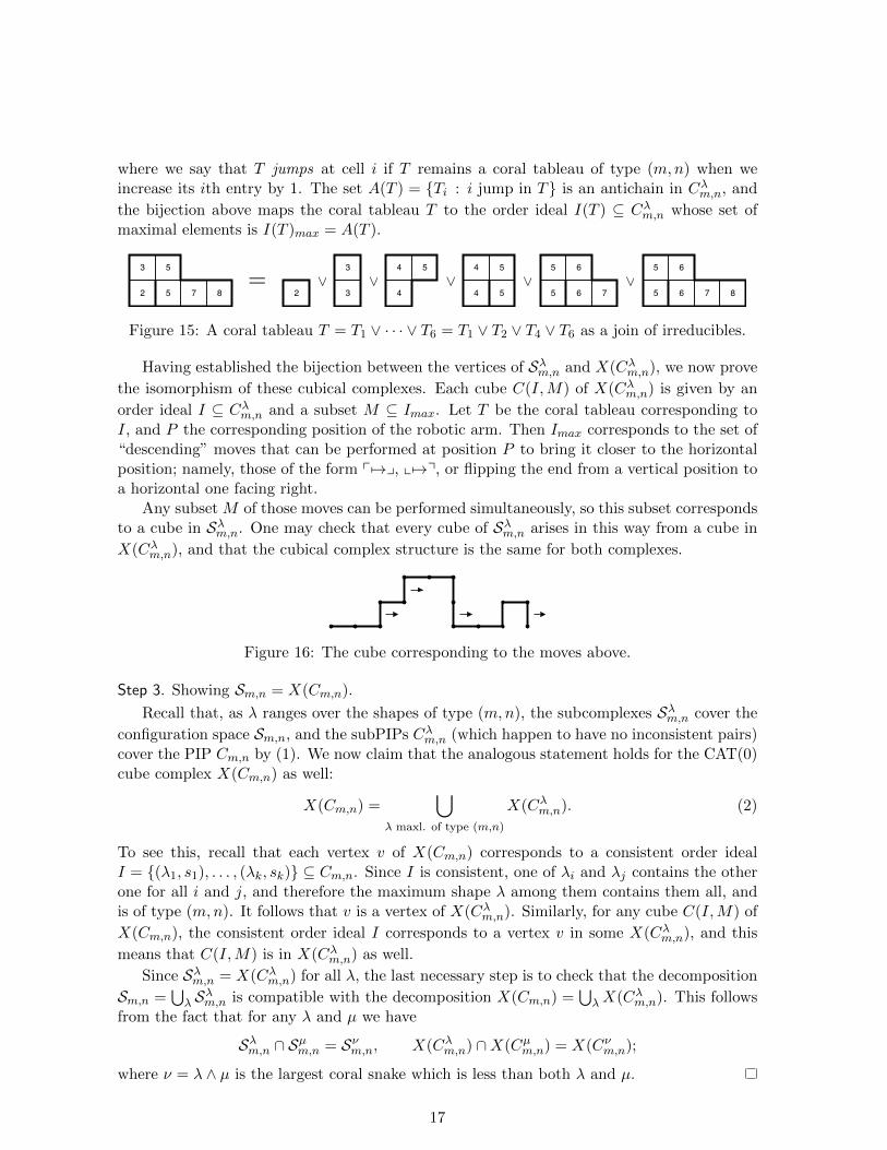
16
where we say that T jumps at cell i if T remains a coral tableau of type (m,n) when weincrease its ith entry by 1. The set A(T ) = {Ti : i jump in T} is an antichain in Cλm,n, and
the bijection above maps the coral tableau T to the order ideal I(T ) ⊆ Cλm,n whose set ofmaximal elements is I(T )max = A(T ).
_ _ _ _ _2
3 5
5 7 8 5
5 6
6 7 85
5 6
6 74
4 5
54
4 5
3
3
2=
Figure 15: A coral tableau T = T1 ∨ · · · ∨ T6 = T1 ∨ T2 ∨ T4 ∨ T6 as a join of irreducibles.
Having established the bijection between the vertices of Sλm,n and X(Cλm,n), we now prove
the isomorphism of these cubical complexes. Each cube C(I,M) of X(Cλm,n) is given by an
order ideal I ⊆ Cλm,n and a subset M ⊆ Imax. Let T be the coral tableau corresponding toI, and P the corresponding position of the robotic arm. Then Imax corresponds to the set of“descending” moves that can be performed at position P to bring it closer to the horizontalposition; namely, those of the form p 7→y, x7→q, or flipping the end from a vertical position toa horizontal one facing right.
Any subset M of those moves can be performed simultaneously, so this subset correspondsto a cube in Sλm,n. One may check that every cube of Sλm,n arises in this way from a cube in
X(Cλm,n), and that the cubical complex structure is the same for both complexes.
Figure 16: The cube corresponding to the moves above.
Step 3. Showing Sm,n = X(Cm,n).
Recall that, as λ ranges over the shapes of type (m,n), the subcomplexes Sλm,n cover the
configuration space Sm,n, and the subPIPs Cλm,n (which happen to have no inconsistent pairs)cover the PIP Cm,n by (1). We now claim that the analogous statement holds for the CAT(0)cube complex X(Cm,n) as well:
X(Cm,n) =⋃
λ maxl. of type (m,n)
X(Cλm,n). (2)
To see this, recall that each vertex v of X(Cm,n) corresponds to a consistent order idealI = {(λ1, s1), . . . , (λk, sk)} ⊆ Cm,n. Since I is consistent, one of λi and λj contains the otherone for all i and j, and therefore the maximum shape λ among them contains them all, andis of type (m,n). It follows that v is a vertex of X(Cλm,n). Similarly, for any cube C(I,M) of
X(Cm,n), the consistent order ideal I corresponds to a vertex v in some X(Cλm,n), and this
means that C(I,M) is in X(Cλm,n) as well.
Since Sλm,n = X(Cλm,n) for all λ, the last necessary step is to check that the decomposition
Sm,n =⋃λ Sλm,n is compatible with the decomposition X(Cm,n) =
where ν = λ ∧ µ is the largest coral snake which is less than both λ and µ.
17
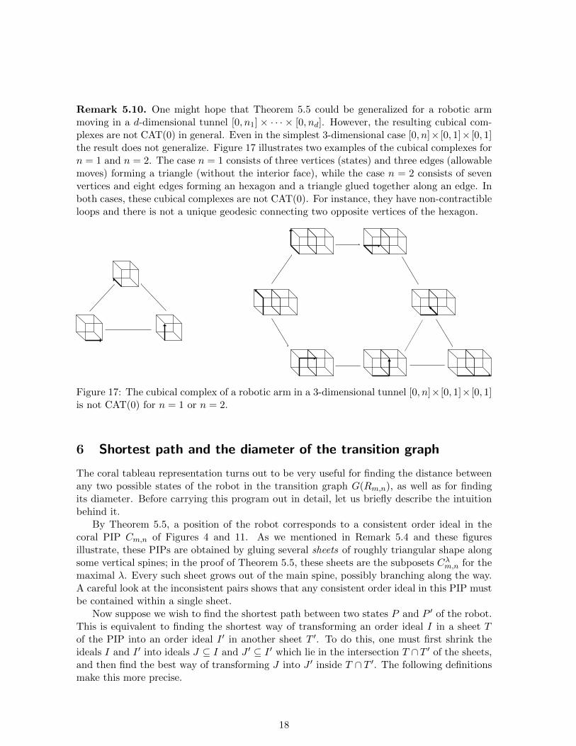
Remark 5.10. One might hope that Theorem 5.5 could be generalized for a robotic armmoving in a d-dimensional tunnel [0, n1] × · · · × [0, nd]. However, the resulting cubical com-plexes are not CAT(0) in general. Even in the simplest 3-dimensional case [0, n]× [0, 1]× [0, 1]the result does not generalize. Figure 17 illustrates two examples of the cubical complexes forn = 1 and n = 2. The case n = 1 consists of three vertices (states) and three edges (allowablemoves) forming a triangle (without the interior face), while the case n = 2 consists of sevenvertices and eight edges forming an hexagon and a triangle glued together along an edge. Inboth cases, these cubical complexes are not CAT(0). For instance, they have non-contractibleloops and there is not a unique geodesic connecting two opposite vertices of the hexagon.
Figure 17: The cubical complex of a robotic arm in a 3-dimensional tunnel [0, n]× [0, 1]× [0, 1]is not CAT(0) for n = 1 or n = 2.
6 Shortest path and the diameter of the transition graph
The coral tableau representation turns out to be very useful for finding the distance betweenany two possible states of the robot in the transition graph G(Rm,n), as well as for findingits diameter. Before carrying this program out in detail, let us briefly describe the intuitionbehind it.
By Theorem 5.5, a position of the robot corresponds to a consistent order ideal in thecoral PIP Cm,n of Figures 4 and 11. As we mentioned in Remark 5.4 and these figuresillustrate, these PIPs are obtained by gluing several sheets of roughly triangular shape alongsome vertical spines; in the proof of Theorem 5.5, these sheets are the subposets Cλm,n for themaximal λ. Every such sheet grows out of the main spine, possibly branching along the way.A careful look at the inconsistent pairs shows that any consistent order ideal in this PIP mustbe contained within a single sheet.
Now suppose we wish to find the shortest path between two states P and P ′ of the robot.This is equivalent to finding the shortest way of transforming an order ideal I in a sheet Tof the PIP into an order ideal I ′ in another sheet T ′. To do this, one must first shrink theideals I and I ′ into ideals J ⊆ I and J ′ ⊆ I ′ which lie in the intersection T ∩T ′ of the sheets,and then find the best way of transforming J into J ′ inside T ∩ T ′. The following definitionsmake this more precise.
18
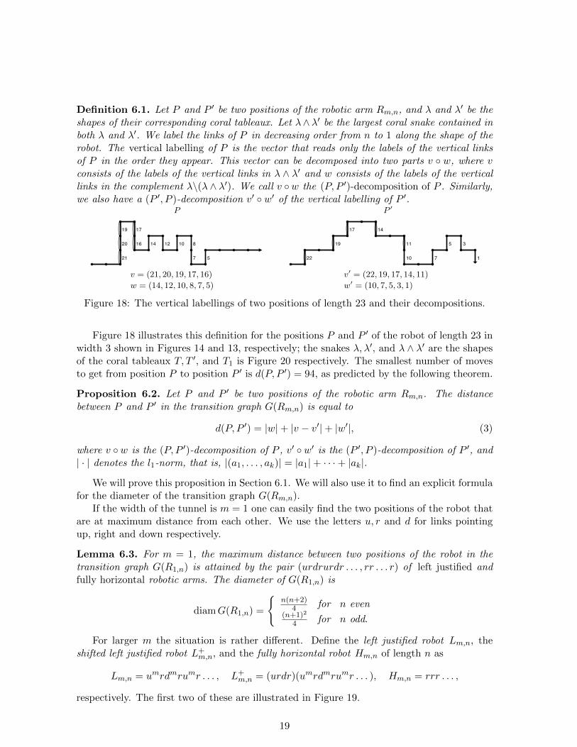
Definition 6.1. Let P and P ′ be two positions of the robotic arm Rm,n, and λ and λ′ be theshapes of their corresponding coral tableaux. Let λ∧λ′ be the largest coral snake contained inboth λ and λ′. We label the links of P in decreasing order from n to 1 along the shape of therobot. The vertical labelling of P is the vector that reads only the labels of the vertical linksof P in the order they appear. This vector can be decomposed into two parts v ◦ w, where vconsists of the labels of the vertical links in λ ∧ λ′ and w consists of the labels of the verticallinks in the complement λ\(λ ∧ λ′). We call v ◦w the (P, P ′)-decomposition of P . Similarly,we also have a (P ′, P )-decomposition v′ ◦ w′ of the vertical labelling of P ′.
22
19
17 14
11
10 7
5 3
157
810121416
1719
20
21
P
v = (21, 20, 19, 17, 16)
w = (14, 12, 10, 8, 7, 5)
P ′
v′ = (22, 19, 17, 14, 11)
w′ = (10, 7, 5, 3, 1)
Figure 18: The vertical labellings of two positions of length 23 and their decompositions.
Figure 18 illustrates this definition for the positions P and P ′ of the robot of length 23 inwidth 3 shown in Figures 14 and 13, respectively; the snakes λ, λ′, and λ ∧ λ′ are the shapesof the coral tableaux T, T ′, and T1 is Figure 20 respectively. The smallest number of movesto get from position P to position P ′ is d(P, P ′) = 94, as predicted by the following theorem.
Proposition 6.2. Let P and P ′ be two positions of the robotic arm Rm,n. The distancebetween P and P ′ in the transition graph G(Rm,n) is equal to
d(P, P ′) = |w|+ |v − v′|+ |w′|, (3)
where v ◦w is the (P, P ′)-decomposition of P , v′ ◦w′ is the (P ′, P )-decomposition of P ′, and| · | denotes the l1-norm, that is, |(a1, . . . , ak)| = |a1|+ · · ·+ |ak|.
We will prove this proposition in Section 6.1. We will also use it to find an explicit formulafor the diameter of the transition graph G(Rm,n).
If the width of the tunnel is m = 1 one can easily find the two positions of the robot thatare at maximum distance from each other. We use the letters u, r and d for links pointingup, right and down respectively.
Lemma 6.3. For m = 1, the maximum distance between two positions of the robot in thetransition graph G(R1,n) is attained by the pair (urdrurdr . . . , rr . . . r) of left justified andfully horizontal robotic arms. The diameter of G(R1,n) is
diamG(R1,n) =
{n(n+2)
4 for n even(n+1)2
4 for n odd.
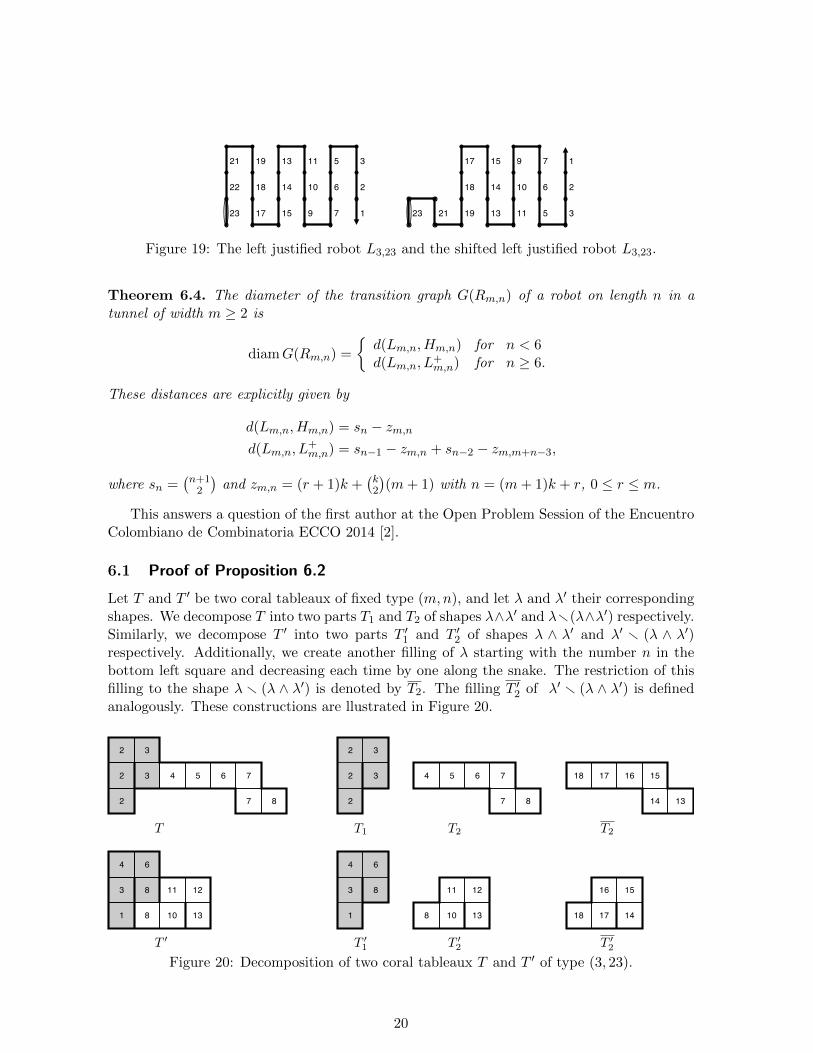
For larger m the situation is rather different. Define the left justified robot Lm,n, theshifted left justified robot L+
m,n, and the fully horizontal robot Hm,n of length n as
respectively. The first two of these are illustrated in Figure 19.
19
23
22
21 19
18
17 15
14
13 11
10
9 7
6
5 3
2
1 23 21 19
18
17 15
14
13 11
10
9 7
6
5 3
2
1
Figure 19: The left justified robot L3,23 and the shifted left justified robot L3,23.
Theorem 6.4. The diameter of the transition graph G(Rm,n) of a robot on length n in atunnel of width m ≥ 2 is
diamG(Rm,n) =
{d(Lm,n, Hm,n) for n < 6d(Lm,n, L
+m,n) for n ≥ 6.
These distances are explicitly given by
d(Lm,n, Hm,n) = sn − zm,nd(Lm,n, L
+m,n) = sn−1 − zm,n + sn−2 − zm,m+n−3,
where sn =(n+12
)and zm,n = (r + 1)k +
(k2
)(m+ 1) with n = (m+ 1)k + r, 0 ≤ r ≤ m.
This answers a question of the first author at the Open Problem Session of the EncuentroColombiano de Combinatoria ECCO 2014 [2].
6.1 Proof of Proposition 6.2
Let T and T ′ be two coral tableaux of fixed type (m,n), and let λ and λ′ their correspondingshapes. We decompose T into two parts T1 and T2 of shapes λ∧λ′ and λr(λ∧λ′) respectively.Similarly, we decompose T ′ into two parts T ′1 and T ′2 of shapes λ ∧ λ′ and λ′ r (λ ∧ λ′)respectively. Additionally, we create another filling of λ starting with the number n in thebottom left square and decreasing each time by one along the snake. The restriction of thisfilling to the shape λ r (λ ∧ λ′) is denoted by T2. The filling T ′2 of λ′ r (λ ∧ λ′) is definedanalogously. These constructions are llustrated in Figure 20.
2
2
2 3
3 4 5 6 7
7 8
1
3
4 6
8
8 10
11 12
13
4 5 6 7
7 82
2
2 3
3
1
3
4 6
8
8 10
11 12
13
18 17 16 15
14 13
18 17
16 15
14
T T1 T2 T2
T ′ T ′1 T ′
2 T ′2
Figure 20: Decomposition of two coral tableaux T and T ′ of type (3, 23).
20
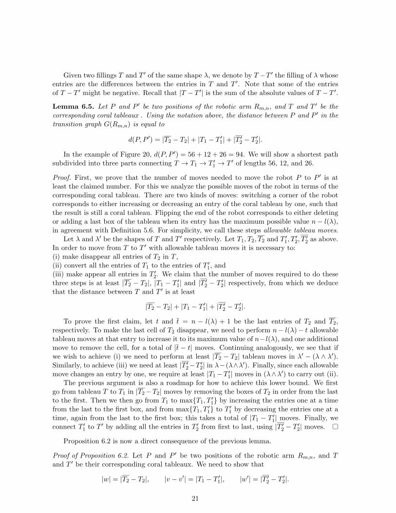
Given two fillings T and T ′ of the same shape λ, we denote by T −T ′ the filling of λ whoseentries are the differences between the entries in T and T ′. Note that some of the entriesof T − T ′ might be negative. Recall that |T − T ′| is the sum of the absolute values of T − T ′.
Lemma 6.5. Let P and P ′ be two positions of the robotic arm Rm,n, and T and T ′ be thecorresponding coral tableaux . Using the notation above, the distance between P and P ′ in thetransition graph G(Rm,n) is equal to
d(P, P ′) = |T2 − T2|+ |T1 − T ′1|+ |T ′2 − T ′2|.
In the example of Figure 20, d(P, P ′) = 56 + 12 + 26 = 94. We will show a shortest pathsubdivided into three parts connecting T → T1 → T ′1 → T ′ of lengths 56, 12, and 26.
Proof. First, we prove that the number of moves needed to move the robot P to P ′ is atleast the claimed number. For this we analyze the possible moves of the robot in terms of thecorresponding coral tableau. There are two kinds of moves: switching a corner of the robotcorresponds to either increasing or decreasing an entry of the coral tableau by one, such thatthe result is still a coral tableau. Flipping the end of the robot corresponds to either deletingor adding a last box of the tableau when its entry has the maximum possible value n− l(λ),in agreement with Definition 5.6. For simplicity, we call these steps allowable tableau moves.
Let λ and λ′ be the shapes of T and T ′ respectively. Let T1, T2, T2 and T ′1, T′2, T
′2 as above.
In order to move from T to T ′ with allowable tableau moves it is necessary to:(i) make disappear all entries of T2 in T ,(ii) convert all the entries of T1 to the entries of T ′1, and(iii) make appear all entries in T ′2. We claim that the number of moves required to do thesethree steps is at least |T2 − T2|, |T1 − T ′1| and |T ′2 − T ′2| respectively, from which we deducethat the distance between T and T ′ is at least
|T2 − T2|+ |T1 − T ′1|+ |T ′2 − T ′2|.
To prove the first claim, let t and t = n − l(λ) + 1 be the last entries of T2 and T2,respectively. To make the last cell of T2 disappear, we need to perform n− l(λ)− t allowabletableau moves at that entry to increase it to its maximum value of n−l(λ), and one additionalmove to remove the cell, for a total of |t − t| moves. Continuing analogously, we see that ifwe wish to achieve (i) we need to perform at least |T2 − T2| tableau moves in λ′ − (λ ∧ λ′).Similarly, to achieve (iii) we need at least |T ′2−T ′2| in λ−(λ∧λ′). Finally, since each allowablemove changes an entry by one, we require at least |T1−T ′1| moves in (λ∧λ′) to carry out (ii).
The previous argument is also a roadmap for how to achieve this lower bound. We firstgo from tableau T to T1 in |T2−T2| moves by removing the boxes of T2 in order from the lastto the first. Then we then go from T1 to max{T1, T ′1} by increasing the entries one at a timefrom the last to the first box, and from max{T1, T ′1} to T ′1 by decreasing the entries one at atime, again from the last to the first box; this takes a total of |T1 − T ′1| moves. Finally, weconnect T ′1 to T ′ by adding all the entries in T ′2 from first to last, using |T ′2 − T ′2| moves.
Proposition 6.2 is now a direct consequence of the previous lemma.
Proof of Proposition 6.2. Let P and P ′ be two positions of the robotic arm Rm,n, and Tand T ′ be their corresponding coral tableaux. We need to show that
|w| = |T2 − T2|, |v − v′| = |T1 − T ′1|, |w′| = |T ′2 − T ′2|.
21
The entry of a box in T2−T2 counts the number of links in P after the corresponding verticallink, including it. Therefore, the entries of w are exactly equal to the entries of T2 − T2.Similarly, the entries of w′ are equal to the entries of T ′2 − T ′2. Now, if v = (v1, . . . , vk)and if (t1, . . . , tk) are the entries of T1 in the order they appear along the snake, then vi =n − (ti + i − 1) for each i. Therefore the entries of v − v′ are exactly the negatives of theentries of T1 − T ′1, and hence |v − v′| = |T1 − T ′1|.
6.2 Proof of Theorem 6.4
Throughout this section we fix m ≥ 2 and n ∈ N. We say that a coral snake λ is of type (m,n)if it appears in the coral PIP Cm,n; that is, if h(λ) ≤ m and l(λ) + w(λ) − 1 ≤ n. All thecoral snakes and positions of the robot considered in this section are of type (m,n).
Definition 6.6. The shape of a position P of the robot, denoted shape(P ), is the shape ofits corresponding coral tableau. The intersection shape of two positions P and P ′ is definedas shape(P ) ∧ shape(P ′).
Our strategy to find the diameter of the transition graph G(Rm,n) is to find the maximumdistance between two positions of the robot with a fixed intersection shape λ, and thenmaximize this quantity over all shapes λ. We need to distinguish two kinds of snakes.
Definition 6.7. A coral snake of type (m,n) is said to be a:• side snake: if the end point of any robot with coral tableau of shape λ is on one of the twohorizontal sides of the tunnel.• middle snake: if it is not a side snake.
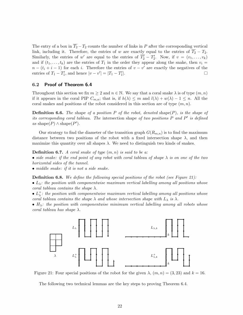
Definition 6.8. We define the following special positions of the robot (see Figure 21):• Lλ: the position with componentwise maximum vertical labelling among all positions whosecoral tableau contains the shape λ.• L+
λ : the position with componentwise maximum vertical labelling among all positions whosecoral tableau contains the shape λ and whose intersection shape with Lλ is λ.• Hλ: the position with componentwise minimum vertical labelling among all robots whosecoral tableau has shape λ.
λ
Lλ
L+λ
Lλ,k
L+λ,k
k
k
Figure 21: Four special positions of the robot for the given λ, (m,n) = (3, 23) and k = 16.
The following two technical lemmas are the key steps to proving Theorem 6.4.
22
Lemma 6.9. The maximum distance between two positions of the robot with fixed intersectionshape λ is:
(i) d(Lλ, Hλ), if λ is a side snake.
(ii) max{d(Lλ, Hλ), d(Lλ, L+λ )}, if λ is a middle snake.
Lemma 6.10. The following hold:
(i) If λ ≺ λ′, then d(Lλ, Hλ) > d(Lλ′ , Hλ′).
(ii) If λ ≺ λ′ are two middle snakes, then d(Lλ, L+λ ) > d(Lλ′ , L
+λ′).
We postpone the proof of these two lemmas for the moment and use them to prove ourmain diameter result.
Proof of Theorem 6.4. By Lemma 6.9, the diameter of the transition graph G(Rm,n) is themaximum between the two values
maxλ
d(Lλ, Hλ), maxmiddle snakes λ
d(Lλ, L+λ ).
By Lemma 6.10, we have
maxλ
d(Lλ, Hλ) = d(L∅, H∅), maxmiddle snakes λ
d(Lλ, L+λ ) = d(L�, L
+�).
where ∅ is the empty snake and � is the snake that consists of only one box. By definition,we have that L∅ = L� = Lm,n, H∅ = Hm,n and L+
� = L+m,n. Therefore,
diamG(Rm,n) = max{d(Lm,n, Hm,n), d(Lm,n, L+m,n)}.
The explicit formulas for these distances stated in Theorem 6.4 are obtained directly fromProposition 6.2. For instance, d(Lm,n, Hm,n) is the sum of all vertical labels in Lm,n. Thissum is equal to the sum sn = 1 + · · · + n of all labels (including the horizontal ones) minusthe sum zm,n of the horizontal labels. The formula for d(Lm,n, L
+m,n) is obtained similarly,
considering the labels of L+m,n as well.
When n ≥ 4, we may rewrite d(Lm,n, L+m,n) = d(Lm,n, Hm,n) + sn−4 − zm,n−4 − 2, which
shows that d(Lm,n, L+m,n) ≥ d(Lm,n, Hm,n) for n ≥ 6 and d(Lm,n, L
+m,n) < d(Lm,n, Hm,n) for
n = 4, 5. The cases n = 1, 2, 3 are easily verified by hand.
6.2.1 Fixing a shape: proof of Lemma 6.9
Let us prove Lemma 6.9 for any fixed coral snake λ of type (m,n). Let P and P ′ be twopositions of the robot with intersection shape λ. We begin by proving case (ii), which is moreintricate, and then return to case (i).
Proof of Lemma 6.9 (ii). Let λ be a middle snake. For `(λ) +w(λ)−1 ≤ k ≤ n the followingspecial positions of the robot (see Figure 21) will play an important role in the proof:
• Lλ,k: the position with componentwise maximum vertical labelling among all positionswhose entries are less than or equal to k and whose coral tableau contains the shape λ .
23
• L+λ,k: the position with componentwise maximum vertical labelling among all positions
whose entries are less than or equal to k, whose coral tableau contains the shape λ, andwhose intersection shape with Lλ,k is λ.
Notice that Lλ,k (resp. L+λ,k) consists of n − k horizontal steps followed by the position
analogous to Lλ (resp. L+λ ) for the robotic arm of length k. In particular, Lλ = Lλ,n
and L+λ = L+
λ,n. The description of the maximum distance between two robots with fixedintersection shape λ will follow from the following three lemmas.
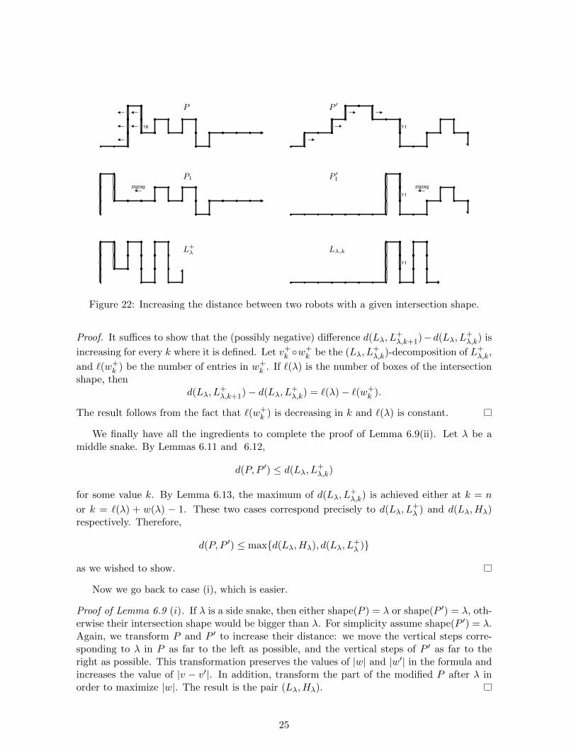
Lemma 6.11. For any positions P and P ′ with intersection shape λ there exists k such thatd(P, P ′) ≤ max{d(Lλ, L
We will perform two distance-increasing transformations to the pair (P, P ′) to obtain either(Lλ, L
+λ,k) or (L+
λ , Lλ,k). Without loss of generality assume that, among the vertical labels inv and v′, the minimum m is achieved in v′.
The first transformation moves the vertical steps corresponding to v in P as far to theleft as possible (by increasing their values in v), and moves the vertical steps correspondingto v′ in P ′ as far to the right as possible (by decreasing their values in v′) while keeping theminimal label equal to m. Denote by P1 and P ′1 the resulting positions; Figure 22 shows anexample. This transformation preserves the values of |w| and |w′| in the formula and increasesthe value of |v − v′|.
The second transformation changes the parts of P1 and P ′1 after their intersection λ, inorder to maximize |w| and |w′| while keeping |v − v′| fixed. We need to keep the intersectionshape equal to λ, so we must respect the up/down direction of the next vertical step in P1 andP ′1 after λ; we convert the rest of P1 and P ′1 into “zigzag snakes” subject to that constraint.The result is either the pair (Lλ, L
+λ,k) or (L+
λ , Lλ,k) for some k. It follows that
d(P, P ′) ≤ d(P1, P′1) ≤ max
{d(Lλ, L
+λ,k), d(L+
λ , Lλ,k)},
as desired. This construction is illustrated in Figure 22.
Lemma 6.12. d(Lλ, L+λ,k) ≥ d(L+
λ , Lλ,k).
Proof. For simplicity, let ` = n− k be the number of initial horizontal steps of Lλ,k and L+λ,k
(if λ is non-empty). As above, label the links of the robot in decreasing order from n upto 1 along the shape of the robot. Let h, h+, hk, h
+k be the restriction of this labelling to the
horizontal links located after the last vertical link corresponding to λ in each of the robotsLλ, L+
λ , Lλ,k, L+λ,k respectively.
The vector h− hk (resp. h+ − h+k ) consists of an initial sequence of (n− k)s followed bythe entries of h (resp. h+) that are less than n − k. Consider the injection taking the ithhorizontal step of Lλ to the ith horizontal step of L+
λ , which has a weakly larger label. Underthis injection, each term of h − hk is dominated by the corresponding term in h+ − h+k . Itfollows that (|h+ − h+k |)− (|h− hk|) ≥ 0.
Lemma 6.13. For a fixed middle snake λ, d(Lλ, L+λ,k) is concave up as a function of k, and
therefore attains its maximum value either at k = l(λ) + w(λ)− 1 or at k = n.
24
1116
11
zigzag zigzag
11
P
P1
L+λ
P ′
P ′1
Lλ,k
Figure 22: Increasing the distance between two robots with a given intersection shape.
Proof. It suffices to show that the (possibly negative) difference d(Lλ, L+λ,k+1)−d(Lλ, L
+λ,k) is
increasing for every k where it is defined. Let v+k ◦w+k be the (Lλ, L
+λ,k)-decomposition of L+
λ,k,
and `(w+k ) be the number of entries in w+
k . If `(λ) is the number of boxes of the intersectionshape, then
d(Lλ, L+λ,k+1)− d(Lλ, L
+λ,k) = `(λ)− `(w+
k ).
The result follows from the fact that `(w+k ) is decreasing in k and `(λ) is constant.
We finally have all the ingredients to complete the proof of Lemma 6.9(ii). Let λ be amiddle snake. By Lemmas 6.11 and 6.12,
d(P, P ′) ≤ d(Lλ, L+λ,k)
for some value k. By Lemma 6.13, the maximum of d(Lλ, L+λ,k) is achieved either at k = n
or k = `(λ) + w(λ) − 1. These two cases correspond precisely to d(Lλ, L+λ ) and d(Lλ, Hλ)
respectively. Therefore,
d(P, P ′) ≤ max{d(Lλ, Hλ), d(Lλ, L+λ )}
as we wished to show.
Now we go back to case (i), which is easier.
Proof of Lemma 6.9 (i). If λ is a side snake, then either shape(P ) = λ or shape(P ′) = λ, oth-erwise their intersection shape would be bigger than λ. For simplicity assume shape(P ′) = λ.Again, we transform P and P ′ to increase their distance: we move the vertical steps corre-sponding to λ in P as far to the left as possible, and the vertical steps of P ′ as far to theright as possible. This transformation preserves the values of |w| and |w′| in the formula andincreases the value of |v − v′|. In addition, transform the part of the modified P after λ inorder to maximize |w|. The result is the pair (Lλ, Hλ).
25
6.2.2 Varying the shape: proof of Lemma 6.10
Proof of Lemma 6.10 (i). By Proposition 6.2, removing the last box of λ increases the dis-tance d(Lλ, Hλ) by `(λ). Therefore λ ≺ λ′ implies d(Lλ, Hλ) > d(Lλ′ , Hλ′).
To prove part (ii) we use a basic lemma.
Lemma 6.14. Let A be a subsequence of (p, . . . , 2, 1) obtained by removing an arithmeticprogression with common difference c, and let A′ be a subsequence of (p′, . . . , 2, 1) obtained byremoving an arithmetic progression with common difference c. If p > p′ then |A| ≥ |A′|.
Proof. Say A and A′ have a and a′ elements, respectively. When listed in decreasing order,the largest a′ terms of A are greater than or equal to the a′ terms of A′. The remaining a−a′terms (if there are any) are positive. Therefore |A| ≥ |A′|.
Proof of Lemma 6.10 (ii). Assume that λ ≺ λ′ are two middle snakes. We need to show thatd(Lλ, L
+λ ) = |w|+|v−v′|+|w′| decreases as we increase λ. The term |v−v′| = 0 stays constant.
The tem |w| clearly does not decrease when we make λ larger. Finally, the term |w′| also doesnot decrease when we make λ thanks to Lemma 6.14. The desired result follows.
7 Implementation of the shortest path algorithm
Since the configuration space of the robotic arm Rm,n is CAT(0), we are able to navigate itthanks to the following theorem.
Theorem 4.2. [1, 3, 11] If the configuration space of a robot is a CAT(0) cubical complex,there is an explicit algorithm to move the robot optimally from one position to another, in:• the edge metric: the number of moves, if only one move at a time is allowed,• the cube metric: the number of steps (where in each step we may perform several physicallyindependent moves),• the time metric: the time elapsed if we may perform independent moves simultaneously.
As shown in [5], there is also a (more complicated) algorithm to move the robot optimallyin terms of the Euclidean metric in the configuration space. However, this metric is lessrelevant, as it does not seem to have a natural interpretation in terms of the robot.
The algorithms of Theorem 4.2 are described in detail in [3]; they are based on the normalcube paths of Niblo and Reeves [10]. We have implemented these algorithms in Python for therobotic arms discussed in this paper. To use the program, the user inputs the width of thetunnel and two positions of the robotic arm of the same length, expressed as sequences of stepsof the form: r (right), u (up), d (down) steps. The program outputs the distance betweenthe two states in the edge metric and in the cube metric3, and an animation taking the robotbetween the two states. The downloadable code, instructions, and a sample animation are athttp://math.sfsu.edu/federico/Articles/movingrobots.html.
3It turns out that the optimal paths in the cube metric are also optimal in the time metric.
• Our robotic arms Rm,n can never have links facing left. Now consider the robotic arm oflength n in a tunnel of width m whose links may face up, down, right, or left, starting inthe fully horizontal position, and subject to the same kinds of moves: switching cornersand flipping the end. Is the configuration space of this robot also CAT(0)? In [4], weshow the answer is affirmative for width m = 2. We believe this is also true for largerm, but proving it in general seems to require new ideas.
• Theorem 6.4 gives the diameter of the configuration space Sm,n in the edge metric, thatis, the largest number of moves separating two positions of the robot Rm,n. What is thediameter of Sm,n in the cube metric, that is, the largest number of steps separating twopositions of the robot Rm,n, where a step may consist of several physically independentmoves?
9 Acknowledgements
This paper includes results from HB’s undergraduate thesis at Universidad del Valle in Cali,Colombia (advised by FA and CC) and JG’s undergraduate project at San Francisco StateUniversity in San Francisco, California (advised by FA). We thank the SFSU-Colombia Com-binatorics Initiative, which made this collaboration possible. We would also like to thank thePacific Ocean for bringing us the beautiful coral that inspired Definition 5.3 and the proof ofour main Theorem 1.6.
References
[1] A. Abrams and R. Ghrist. State complexes for metamorphic robots. Int. J. Robotics Res.23 (2004) 811-826.
[2] F. Ardila. Open Problem Session, Encuentro Colombiano de Combinatoria, Bogota, 2014.
[3] F. Ardila, T. Baker, and R. Yatchak. Moving robots efficiently using the combinatoricsof CAT(0) cubical complexes. Adv. in Appl. Math. 48 (2012) 142-163.
[4] F. Ardila, H. Bastidas, C. Ceballos, and J. Guo. The configuration space of a robotic armin a tunnel of width 2. To appear in the Proceedings of Formal Power Series and AlgebraicCombinatorics (FPSAC 2016), Discrete Mathematics and Theoretical Computer Science.
[5] F. Ardila, M. Owen, and S. Sullivant. Geodesics in CAT(0) cubical complexes. SIAM J.Discrete Math. 28-2 (2014) 986-1007.
[6] G. Birkhoff. Rings of sets. Duke Mathematical Journal 3 (1937) 443-454.
[7] M. Bridson and A. Haefligher. Metric spaces of non-positive curvature. Springer-Verlag,Berlin, Heidelberg, 1999.
[8] R. Ghrist and V. Peterson. The geometry and topology of reconfiguration. Adv. in Appl.Math. 38 (2007) 302-323.
27
[9] M. Gromov. Hyperbolic groups. In Essays in group theory, volume 8 of Math. Sci. Res.Inst. Publ. 75-263. Springer, New York, 1987.
[10] G.A. Niblo and L.D. Reeves. The geometry of cube complexes and the complexity oftheir fundamental groups. Topology, 37(3) (1998) 621-633.
[11] L. D. Reeves. Biautomatic structures and combinatorics for cube complexes. Ph.D. thesis,University of Melbourne, 1995.
[12] M. A. Roller. Poc sets, median algebras and group actions. an extended study of Dun-woody’s construction and Sageev’s theorem. Unpublished preprint, 1998.
[13] M. Sageev. Ends of group pairs and non-positively curved cube complexes. Proc. LondonMath. Soc. (3), 71 (3) 585-617, 1995.
[14] L. Santocanale. A nice labelling for tree-like event structures of degree 3. Inf. Comput.,208:652-665, 2010.
[15] G. Winskel. Event Structures. Advances in Petri Nets 1986. Springer Lecture Notes inComputer Science 255, 1987.