A THEORY OF OCCUPATIONAL CHOICE WITH ENDOGENOUS FERTILITY

Dilip Mookherjee1, Silvia Prina2 and Debraj Ray3

November 2010

Abstract

This paper studies the steady states of a model which combines endogenous fertility with oc-

cupational choice. Three sets of results are obtained. (a) There is a negative cross-sectional

relationship between parental wages in different occupations and fertility, independent of the

relative strength of wealth and substitution effects that determine fertility in the standard frame-

work. (b) The differential fertility across occupational categories creates Intergenerational mo-

bility in steady state. Unlike mobility created by stochastic shocks, such occupational drift

has a predictable direction depending on the income-fertility relationship. (c) Steady states are

(generically) locally determinate and permit the analysis of various policy changes.

1. Introduction

The connections between economic conditions and fertility have been well recognized since

the time of Malthus. These links have been explicitly explored by Becker (1960), Becker

and Barro (1986, 1988), and Barro and Becker (1989). The Barro-Becker approach as-

sumes parental preferences over the number and well-being of their offspring, integrated

into a representative-agent optimal growth model. A sizable literature has emerged from

these papers, including extensions that incorporate human capital, agent heterogeneity

and inequality (e.g., Becker, Murphy and Tamura (1990), Sah (1991), Dahan and Tsiddon

(1998), Alvarez (1999), Kremer and Chen (1999, 2002), Galor and Weil (2000), De La

1Boston University2Case Western University3New York University

1

2

Croix and Doepke (2003), Doepke (2004, 2005), Jones, Schoonbroodt and Tertilt (2008),

and Jones and Schoonbroodt (2009)).

Parent-child interaction is not limited to fertility decisions. The theory of occupational

choice emphasizes how educational investment decisions made by parents condition the

occupational choices of their children. When financial markets are missing or incom-

plete, such theories generate persistent inequality and history dependence (e.g., Banerjee

and Newman (1993), Galor and Zeira (1993), Ljungqvist (1993), Freeman (1996), Aghion

and Bolton (1997), Bandopadhyay (1997), Lloyd-Ellis and Bernhardt (2000), Matsuyama

(2000, 2003), Ghatak and Jiang (2002) and Mookherjee and Ray (2002, 2003, 2010)).

However, this literature is not concerned with fertility.

We combine the theory of endogenous fertility with a theory of occupational choice.4 As

in the endogenous fertility literature, parents decide how many children to have. As in the

occupational choice literature, parents make investments in the future of their children, and

market forces endogenously pin down the returns to different occupations. The interaction

between fertility and human capital investments generates a number of novel results, which

we now discuss.

A central goal of the endogenous fertility literature is to explain the demographic transition.

Fundamental to that transition is the fall in fertility with economic development. Arguably

the most important component of “development” is an improvement in the economic well-

being of parents; see Barro and Becker (1989), Alvarez (1999), Kremer and Chen (1999,

2002), Galor and Weil (2000) and Greenwood and Seshadri (2002).5 This is the cross-

sectional relationship that we study in this paper.

4A number of the papers on endogenous fertility cited above incorporate human capital and inequality,such as Dahan and Tsiddon (1998), Kremer and Chen (1999, 2002), de la Croix and Doepke (2003) andDoepke (2004). So in a broad sense, we are not the first to do this. But there are distinctive elements ofour approach, which include the endogenous determination of steady states as in the occupational choiceliterature, the use of general equilibrium properties of those steady states as a key source of the mainresults (rather than restrictions on preferences), and an explicit consideration of the link between fertilityand inter-occupational mobility. Section 8 discusses the relation of this paper to the existing literature inmore detail.5In related exercises, one might study the effect of a reduction in infant or child mortality on fertility (see,e.g., Sah (1991) and Doepke (2005)), or the effects of anticipated improvements in child welfare on fertilitychoices (see, e.g., Jones and Schoonbroodt (2009)).

3

Is the empirical relationship between parental wages and fertility systematically negative?

It is fair to say that the answer is generally in the affirmative. In their excellent overview

of the literature, Jones, Schoonbroodt and Tertilt (2008) summarize the empirical cross-

sectional correlations between parental income and fertility in developed countries. Most

studies find a negative relationship. At the same time, while widespread, the relationship

is not universal. In some contexts, e.g., in various agrarian settings, there is systematic

evidence of a positive relationship. Studies include Simon (1977) for Poland in 1948; Clark

(2005), Clark and Hamilton (2006), and Clark (2007) for England in the 16th and 17th

century; Weir (1995) for France in the 18th century; Wrigley (1961) and Haines (1976) for

some areas in France and Prussia in the 19th century; and Lee (1987) for the U.S. and

Canada. Schultz (1986) reports that empirical studies of fertility have shown a negative

relationship between male wages and fertility in high-income urban populations but a

positive one in low-income agricultural populations. Even within urban populations in

developed countries, a positive relationship has been found within particular segments.

For example, in the context of the US, Blau and van der Klaauw (2007) find a negative

effect of wages on fertility for white male wage earners, but a positive effect for Blacks

and Hispanics. Freedman (1963) found a positive effect of “relative income” of fertility

within particular occupational categories. Specifically, within the same occupation, higher

income households tend to have more children, whilst average fertility varies negatively

with income across occupations. This is consistent with views expressed earlier by Spengler

(1952) and Easterlin (1973) that fertility growth is positively related to relative incomes

within an occupational category.6

Motivated by the overall negative relationship between parental wages and fertility, medi-

ated by a possibly different pattern within occupations, this paper isolates and compares

different factors that work both within and across occupational categories. Theories of

endogenous fertility run into a ubiquitous problem that we, too, must confront: a clear-

cut prediction invariably depends on the interaction of wealth and substitution effects in

parental preferences. The net effect is generally unclear. The wealth effect captures the

6Simon (1969) points out that over the course of the business cycle the correlation of fertility with incometends to be positive, in contrast to the cross-sectional pattern, also possibly for these reasons.

4

tendency to acquire more children (much like consumer durables) with rising earnings. The

substitution effect captures the higher time costs of childrearing: e.g., increased participa-

tion in the labor market by women. This effect will work to reduce fertility, in line with

observed outcomes. For a large and reasonable class of preferences, one obtains a net pos-

itive correlation between parental wages and fertility.7 To get around this problem, most

models impose strong assumptions on preferences that restrict the relative magnitude of

wealth effects. Within the family of constant-elasticity utility functions, to obtain a nega-

tive relationship, one needs to rule out functions that exhibit at least as much curvature as

the logarithmic function. As Jones and Schoonbroodt (2009) point out, calibrated values of

intertemporal elasticities of substitution in the utility function that fit central qualitative

aspects of the demographic transition, happen to be inconsistent with parameter values

used in growth and business-cycle applications.

Our emphasis on occupational choice yields an alternative way of modeling the cross-

sectional parental wage-fertility correlation which turns out to be consistent with the em-

pirical findings. We employ the Barro-Becker formulation of parental altruism, in which

the strength of parental preferences for children are driven by the lifetimes utilities enjoyed

by offspring. We do not impose strong parameter restrictions on parental preferences that

restrict the strength of wealth effects relative to substitution effects. When wealth effects

are dominant (in the sense of exhibiting at least as much curvature as the logarithmic

function), the resulting wage-fertility correlation will indeed be positive, provided that the

parental wage variation induces no change in the occupational choice of progeny. However,

whenever a high parental wage induces a switch to higher occupational choices, there is

an associated robust drop in fertility which is entirely independent of the relative strength

of income and substitution effects. It arises from the way in which an induced trade-off

between parental preferences for quality and quantity of children must be resolved, when

there is an occupational shift. Our formulation is therefore consistent with a fertility drop

across occupations, coupled with ambiguous outcomes within occupations.

7Indeed, Becker (1960) claimed that the wealth effect was typically dominant. For Becker and others, thenegative cross-sectional relationship was an artifact, caused by ignorance of contraceptive methods on thepart of low-income individuals.

5

The heart of the subsequent analysis is a steady state comparison of overall fertility across

skilled and unskilled occupations, which combines the two effects described above. With

high curvature of utility the two are in mutual opposition: the “preferences effect” tends

to raise fertility; the “occupational shift effect” tends to lower it. Our first main result is

that, for a large range of constant elasticity utility functions (including those with arbi-

trarily large wealth effects), the occupational shift effect outweighs the preference effect,

as a consequence of the endogenous determination of skilled and unskilled wages in steady

state. In particular, in the leading special case in which when child-rearing costs involve

parental time alone, we obtain a declining relationship between fertility and (endogenously

determined) parental incomes, for all constant elasticity utility functions. Whenever the

empirical setting allows substantial variations in occupations or human capital — as in

urban settings in modern societies — our theory thus predicts a negative cross-sectional

correlation quite generally. But when we look within occupations of modern urban soci-

eties, or examine settings (such as traditional agrarian societies) not associated with major

variations in occupations or education, this result may get reversed if wealth effects are

strong.

In their 2008 survey, Jones, Schoonbroodt and Tertilt describe two other routes to a neg-

ative cross-sectional relationship. One of them relies on endogenous human capital invest-

ments (e.g., Becker and Tomes (1976) and Moav (2005)), as we do here. But there are

fixed rates of return to human capital in these models, and restrictions must be assumed in

order for the desired result to work. In contrast, our approach is based on a general equilib-

rium argument, using the discipline imposed by a steady state. These general equilibrium

factors limit the extent to which skilled wages exceed unskilled wages, and thus restrict

the scope of a positive (net) correlation arising from preferences alone. A second route

reverses the causality: with heterogeneous agents, parents with a greater taste for higher

fertility will have more children, adversely affecting their own human capital acquisition in

the process. In our approach, the human capital (or occupation) of parents is determined

before they make fertility and educational decisions. This is particularly pertinent to de-

veloping countries with low average levels of educational attainment, in which most of the

6

population do not complete secondary schooling. In any case, the reversal of causality,

while interesting in its own right, emphasizes a route, not the one that we might focus

on from the perspective of the demographic transition, in which the change in economic

circumstances is presumably the factor that drives fertility outcomes.

The second main contribution of this paper is to the theory of intergenerational mobility.

Existing theories of mobility rely on stochastic shocks to abilities or incomes, and assume

constant, exogenous fertility (e.g. Becker and Tomes (1979), Loury (1981), Banerjee and

Newman (1993) and Mookherjee and Napel (2007)). We show that incorporating endoge-

nous fertility induces mobility even in the absence of any stochastic shocks. More generally,

mobility levels in steady state depend on fertility patterns. If fertility is higher in unskilled

occupations, the proportion of skilled agents in the economy will tend to drift downwards

over time. A steady state in which per capita skill in the economy is constant over time

therefore requires upward mobility: a fraction of unskilled households must decide to ed-

ucate their children to prepare them for entry into the skilled occupation. A society with

a higher fertility differential between the skilled and unskilled must therefore also involve

greater mobility. The possible connection between mobility and fertility patterns has been

overlooked in the existing literature on intergenerational mobility (see, e.g. the symposium

in the Journal of Economic Perspectives 2002, 16(3)).

This leads to the third contribution of the paper. By the logic sketched above, steady

states with differential fertility across occupations must be associated with the indifference

of parents in one occupational category between educating and not educating their children.

A positive fraction of parents must decide not to educate their children in order to ensure

that there will be positive supply of unskilled workers in the next generation. At the same

time a positive fraction must also decide to educate their children, in order to ensure steady-

state constancy of the skill ratio. This indifference condition ties down relative wages

and hence the skill ratio in steady state, ensuring local determinacy of macroeconomic

aggregates and the level of inequality. This is in marked contrast to occupational choice

models with exogenous and constant fertility, which typically exhibit a continuum of steady

states. Hence, endogenizing fertility eliminates the extreme hysteresis of these models, and

7

limits the extent of long-run history dependence: small macro shocks will not generally

have permanent effects. Moreover, it permits the analysis of policy questions. Our theory

generates predictions about the macroeconomic effects of childcare or education subsidies,

redistributive tax-transfer policies or child labor regulations.8 Specifically, a rise in the

non-time component of childcare costs, or a fall in education costs, or stronger child labor

regulations, are shown to increase long run human capital investments, raising per-capita

income and lowering wage inequality across skilled and unskilled occupations. The same

effects obtain with a reduction in unconditional transfers to the unskilled that are funded by

taxes on earnings of the skilled, or an increase in transfers conditioned on school enrollment

of children.

The paper is organized as follows. Section 2 introduces the model. Section 3 makes

the distinction between partial and general equilibrium effects in the study of fertility

decline. Section 4 analyzes household optimal choices in the partial equilibrium setting

with given wages and continuation values of children. Following this, Section 5 introduces

steady states, and establishes our results concerning mobility in steady state. Section 6

studies conditions under which the general equilibrium of steady states yields a negative

wage-fertility correlation. Section 7 then shows steady states are locally determinate and

performs comparative static exercises.

2. Model

2.1. Occupations and Technology. A single output is produced under competitive con-

ditions, using skilled and unskilled labor. Let λ denote the fraction of skilled labor. The

marginal product of skilled labor decreases in λ; the opposite is true of unskilled labor.

Both marginal products are smooth functions of λ and satisfy Inada endpoint conditions.9

There are two occupations, unskilled (0) and skilled (1). Skilled workers can work as either

unskilled or unskilled labor, a choice not available to unskilled workers. Let λ denote the

8It is worth noting the contrast with Barro and Becker (1989) in which long run policies tend not to haveany long run effects, owing partly to the assumption of a perfect capital market in their model. In opposingcontrast, Mookherjee and Ray (2008) use an occupational choice model with exogenous fertility to studylong-run effects of tax-transfer policies, and have to resort to non-steady-state analysis.9That is, they go to ∞ and 0 at either end of their variation.

8

value of λ for which the marginal products of skilled and unskilled labor are equalized.

Then for λ < λ, skilled and unskilled wages (w1 and w0) equal their respective marginal

products, while for higher skill ratios they both equal the common marginal product at λ.

2.2. Fertility, Childrearing and Education. There is a continuum of households at

every date, with one adult (a single parent) in each household.10 A parent earns a wage w

on the labor market and chooses how many children n to have, where we suppose n to be

a continuous variable.11

Child-rearing and education are costly activities. We distinguish between the cost incurred

in raising an unskilled child — r0(w) — and the cost of raising a skilled child — r1(w).

We maintain the following assumptions on r0 and r1 throughout the paper:

[R.1]. For each category i = 0, 1, ri(w) is smooth and strictly increasing in w, while ri(w)w

is nonincreasing. There is a positive lower bound r to the rate of increase of ri, i = 0, 1.

[R.2]. For every w, r1(w) > r0(w).

[R.3]. For every w,r�1(w)

r1(w)<

r�0(w)

r0(w).

Assumption R.1 states that higher parental wages increase child-rearing costs, but less

than proportionately. The former arises from the time component to child-rearing which

causes the parent to be away from work.12 Other fixed resource costs of child-bearing and

rearing would be independent of parental wages, which would imply that per-child costs

would rise less than proportionately with parental wages. Note that R.1 allows such fixed

costs to be zero.13 Assumption R.2 is self-evident: imparting skills to children is costly.

10It is possible with no great gain in insight to extend the model to two parents per household.11Conceivably, similar results can be obtained in a model with integer-valued family size and cross-household heterogeneity in parental fertility preferences, where we can interpret the n obtained in thecurrent theory as the average number of children (conditional on parental economic status) that wouldarise in the richer model. Whether and when such “purification” can be achieved is a question for futureresearch.12This formulation is compatible with the possibility that skilled parents find it easier to educate theirchildren, but we assume that the net monetary cost still rises with the wage.13Our result concerning existence of interior steady states, however, does require the assumption of positivefixed costs.

9

Assumption R.3 states that the marginal cost impact of a higher parental wealth (relative

to the overall upbringing budget) is lower for skilled children than for unskilled children.

Suppose, for instance, that there is a child-rearing component k(w), and an additional

cost s(w) of imparting skills (“k” for kids, “s” for skills). Then r0(w) = k(w) and r1(w) =

k(w)+ s(w), and (R.1)–(R.3) are met provided that k and s are increasing and k(w)/s(w)

increases in w. In particular, (R.1)–(R.3) hold if s(w) equals some fixed constant. Call

this cost structure separable.

An important subcase of the separable structure is one in which rearing each child involves

a certain amount of parental time alone. Then k(w) = ψw for some ψ > 0. We will use

this for one of the main results.14

While the functions r0 and r1 are exogenous to the model, they can be influenced by policies

pertaining to child-care subsidies, child labor regulations and costs of family planning.

Section 5 of the paper will examine these effects.

Unlike most preceding models of fertility, we allow parents to educate some children but not

others. Let e be the fraction of children made skilled; then total expenditure on children

is given by r(w, e) ≡ er1(w) + (1− e)r0(w), so that the lifetime consumption of the parent

is equal to

c = w − r(w, e)n,

which we constrain throughout to be nonnegative. This reflects the underlying credit

constraint common to all occupational choice models, wherein education or child-rearing

costs cannot be financed by borrowing and must entail consumption sacrifices made by

parents.

2.3. Preferences. Each parent possesses, first, a utility indicator defined on lifetime con-

sumption c, given by u(c). The parent also derives utility from the lifetime payoff V to

be enjoyed by each child. These latter values will be endogenous to the model and will be

14Another relevant subcase is one where k(w) = f +ψw, the sum of a fixed goods cost and maternal timecosts.

10

solved for in equilibrium. We write the overall payoff to a parent as

(1) u(c) + δnθ [eV1 + (1− e)V0] .

where δ is the cross-generational discount factor, nθ is a weighting factor that depends on

the total number of children n, e is the proportion of children who are skilled, and Vj is

the expected lifetime values accruing to an individual who is placed in skill category j.

As in all the literature, we presume that, controlling for their own consumption and for

child utility, parents prefer more children to less.15 This means that θ and the value

functions (and consequently the utility function u) must have the same sign. We therefore

assume that

[U.1]. u is smooth, increasing, strictly concave, and has unbounded steepness when con-

sumption is zero.

[U.2]. θ �= 0, and θ < 1.

[U.3]. u is nonnegative throughout when θ > 0, and negative throughout when θ < 0.

[U.4]. 0 < δ < rθ.

[U.1] is standard. In [U.2], the restriction that θ �= 0 means that parents are sensitive

to family size, while the assumption that θ < 1 reasonably imposes diminishing marginal

returns to family size.16 [U.3] embodies the discussion that follows equation (1) above. And

[U.4] constrains the discount factor so as to ensure that value functions are stationary. In

particular, the non-negativity of parental consumption and [R.1] ensure an upper bound

1r to fertility.17 Hence [U.4] ensures that δnθ always lies between 0 and 1.

Jones and Schoonbroodt (2009) contains more discussion on the joint restrictions that link

θ and u, and on the need for u to have a single sign (thereby ruling out, say, the case

15We hasten to add that this does not mean that parents will unconditionally prefer more children to less!But it does exclude the case in which parents believe that never having been born is a better option thanlife.16No corresponding restriction on θ needs to be imposed when it is negative.17By [R.1], child-rearing costs are at least r.wn, so parental consumption is at most w[1− r.n].

11

of logarithmic preferences). They — and most of the contributors to the literature on

endogenous fertility — find it convenient to work with the case in which u has constant

elasticity:

u(c) =c1−ρ

1− ρ,

where ρ is positive but not equal to 1, this last restriction ensuring that we are always in

either the positive or the negative utility case. Accompanying restrictions need to be placed

on θ: it must have the same sign as 1 − ρ. This is used in our main result (Proposition

9) concerning steady state characterization, though not for other results concerning the

optimal fertility behavior of parents, or for the comparative statics results.

3. The Income-Fertility Relationship: Some Conceptual Issues

Suppose that we study fertility change over the parental cross-section, by examining a

variety of parental incomes and associated fertility choices. This examination can be

decomposed into two distinct parts.

First, there is the “partial equilibrium” effect, in which wages at different occupations are

given, now and for the next generation. As we move over different parental incomes, we

would allow parents to re-optimize, not just with respect to fertility but also with respect

to occupational choice for their children. This is the exercise that we carry out in the next

section, Section 4.

Second, there is the “general equilibrium” effect, in which the wages for different occupa-

tions are endogenously determined via market conditions. As far as the model goes, then,

we would generate the wage observations at different points on the equilibrium cross-section

of occupational categories, and the question is whether these equilibrium observations ex-

hibit declining fertility at higher parental incomes. This is the subject of Section 5.

4. The Partial Equilibrium of Fertility Decline

4.1. The Occupational Shift Effect. In this section, we identify an effect that invariably

works in favor of fertility decline as parents move their children from unskilled to skilled

occupations. Because such a shift is also correlated with higher parental income, this

12

creates what we call an “occupational shift effect” that relates parental income negatively

to fertility, entirely independent of the specific structure of preferences.

Fix lifetime values V1 and V0 for children, with V1 > V0. Denote by n(w, e) the optimal

choice of n when wealth is w and the proportion of skilled children is e.18 Using the

first-order condition with respect to n,

(2) u� (w − r(w, e)n(w, e)) r(w, e) = θn(w, e)θ−1 [eV1 + (1− e)V0] .

This condition defines the function n(w, e) uniquely at all w > 0.19

With n(w, e) determined in this way, we can express parental utility as a function of e

alone:

V (w, e) ≡ u (w − r(w, e)n(w, e)) + n(w, e)θ [eV1 + (1− e)V0]

= u (w − r(w, e)n(w, e)) +1

θu� (w − r(w, e)n(w, e)) r(w, e)n(w, e),(3)

where the second equality invokes the first-order condition (2). This expression allows us

to establish the first of two basic propositions that underpin the paper.

Proposition 1. Under positive utility, the agent always acts as if she maximizes total

expenditure on children, r(w, e)n(w, e), by choosing e, given n.

Under negative utility, the agent always acts as if she minimizes r(w, e)n(w, e) by choosing

e, given n.

Proof. First note that the expression

(4) u(w − z) +u�(w − z)z

θ

18For now we suppress the dependence of fertility on V1, V0 and other parameters. These will be madeexplicit whenever needed.19Obviously, n(0, e) = 0. Also, note that the second-order condition for this maximization problem —given e — is always met. We approach the joint determination of e and n in the main text to follow.

13

is strictly increasing in z under positive utility, and is strictly decreasing in z under negative

utility. To see this, note that the derivative of the expression above equals�1

θ− 1

�u�(w − z)− u��(w − z)z

θ,

which is strictly positive in z under positive utility and strictly negative in z under negative

utility.

To complete the proof compare V (w, e) (as in the second line of (3)) with the expression

in (4), by setting z = r(w, e)n(w, e).

The proposition states that the a parent’s choice of occupational mix follows a simple

criterion of finding an extremal value for total child-related expenditures. She maximizes

such expenditure (by choice of e) when utility is positive and minimizes it when utility is

negative.

This property, which plays a key role, should not be misunderstood. It does not state that

a parent maximizes or minimizes expenditure on children by choosing e and n. Rather,

it states that a parent maximizes or minimizes expenditure through the choice of e alone,

under the artificial presumption that she “then” chooses fertility n to maximize overall

payoff.

Our second proposition states that a parent invariably finds it optimal to educate all or

none of her children.

Proposition 2. A parent must always set e equal to 0 or 1.

Proof. For any given value of w, set x ≡ r1(w) − r0(w) > 0. Differentiate the first line of

(3) with respect to e and use the envelope theorem to get

∂V (w, e)

∂e= n(w, e)θ(V1 − V0)− u�(w − r(w, e)n(w, e))xn(w, e),

and now use the first-order condition (2) to write this as

(5)∂V (w, e)

∂e=

n(w, e)θx

r(w, e)

��r0(w)

x+ (1− θ)e

�(V1 − V0)− θV0

�.

14

Of course, if V1 ≤ V0, e = 0 is optimal. If V1 > V0 then (5) proves that V is strictly

quasiconvex in e, for given w. It follows that no interior solution to e can ever maximize

V .

Propositions 1 and 2 immediately imply

Proposition 3. Consider any wage w∗ at which the parent is indifferent between e = 0

and e = 1. Then the expenditures on children must be equalized at such a wage:

(6) r1(w∗)n(w∗, 1) = r0(w

∗)n(w∗, 0).

In particular, n(w∗, 1) < n(w∗, 0) at a point of indifference.

Note that this proposition assures us of a fertility decline as soon as a dynasty crosses

occupational boundaries towards higher skills. In contrast, in the traditional Barro-Becker

setting the question of whether a fertility decline occurs with higher wealth depends on

wealth versus substitution effects. We illustrate this further below.

A comparison of the “traditional” effect, which occurs over continuous changes in wage,

and the effect in Proposition 2, which addresses the discontinuous crossing of occupational

boundaries, is a principal theme of the paper. To set the stage for this analysis, we record

the following single-crossing property:

Proposition 4. Suppose that both e = 0 and e = 1 are optimal for some parental wage

w∗. Then e = 1 (resp. e = 0) is the unique optimum choice of e for all higher (resp.

lower) wages.

Proof. Define

∆(w) = u (w − r1(w)n(w, 1)) + n(w, 1)θV1 − u (w − r0(w)n(w, 0))− n(w, 0)θV0

and differentiate with respect to w, evaluating the result at any point such that ∆(w) = 0.

By the envelope theorem applied to n(w, 1) and n(w, 0), we have that

∆�(w) = u� (w − r1(w)n(w, 1)) [1− r�1(w)n(w, 1)]−u� (w − r0(w)n(w, 0)) [1− r�0(w)n(w, 0)].

15

By Proposition 3, the terms within the two u�s are exactly equal. It follows that the sign

of ∆�(w) equals the sign of

r�0(w)n(w, 0)− r�1(w)n(w, 1) =r�0(w)

r0(w)r0(w)n(w, 0)−

r�1(w)

r1(w)r1(w)n(w, 1).

By Proposition 3, we have r0(w)n(w, 0) = r1(w)n(w, 1). Applying (R.3), we see that

∆�(w) > 0 at any point of indifference between e = 0 and e = 1, which completes the

proof.

We summarize these propositions. Proposition 2 tells us that parents either leave all their

children unskilled, or find it optimal to educate them all; there are no halfway measures.

This makes it possible to discuss the notion of an “occupational shift”, in which parents

switch at some threshold to educating all their children. Proposition 3 proves that at

that shift, fertility must undergo a discrete jump downwards. Proposition 4 shows that

the switch occurs as parental wages increase. Taken together, these propositions identify

a neighborhood of parental wages over which the cross-sectional relation between fertility

and parental wages is discretely, and therefore decisively, negative. This is the occupational

shift effect.

4.2. The Traditional Preference-Based Effect. On either side of the occupational-

shift threshold, however, the reaction of fertility to a change in parental wages is given by

the conventional conflict between wealth and substitution effects. To describe this tradeoff

in the clearest possible way, assume that the utility indicator u displays constant elasticity,

so that

u(c) =c1−ρ

1− ρ,

where ρ is positive but not equal to 1. Presume, moreover, that for each occupational

category i, rearing/educational costs are of the form

ri = fi + ψiw,

where fi ≥ 0 and ψi ∈ (0, 1). Let �i(w) ≡ ψiw/(fi + ψiw) be the elasticity of ri with

respect to its argument w.

16

Proposition 5. Fix an occupation i with given wage for the children. Then ni ≡ n(w, i)

is locally increasing in parental wage w if

(7) ρ >�i(w)− ψini

1− ψini,

and locally decreasing if the opposite inequality holds. In particular, if ρ > 1, then fertility

is strictly increasing in parental wage.

Proof. Study the first order condition (2), and note that the right-hand side of this con-

dition is independent of w, while it is strictly decreasing in n.20 Therefore ni is locally

increasing in w if the derivative of the left-hand side of (2) with respect to w is negative,

or equivalently, if

u�(c)r�(w) + u��(c)r(w)[1− nr�(w)] < 0,

and is decreasing if the opposite inequality holds. After noting that 1 − ψini ≥ 1 − (fi +

ψi)ni = ci/w > 0, it is easy to see that this expression reduces to condition (7).

Note that �i(w) ≤ 1, so as long as ρ > 1, fertility must increase with parental income.

Proposition 5 summarizes the familiar tussle between wealth and substitution effects that

makes it so difficult to generate an unambiguous prediction of fertility decline in the Barro-

Becker model. For instance, in the case in which there are no “material costs” of rearing

children, we have fi = 0 and �i(w) = 1, so that the condition in (7) reduces precisely to

ρ > 1 for fertility to increase with wages, and to ρ < 1 to get declining fertility. This latter

condition corresponds to a high elasticity of intertemporal substitution in consumption.

But as Jones and Schoonbroodt (2009) have noted, such high elasticities of intertemporal

substitution are at odds with what is assumed in the literature on growth and business

cycle theory.

When condition (7) is met, the income effects associated with rising parental wages out-

weigh the associated substitution effects, and fertility must rise with wages on either side

of the threshold w∗ for an occupational shift. This is in contrast to the discrete drop in fer-

tility at the threshold. In short, the behavior of fertility across parental wages within each

20Note that continuation value V and θ have the same sign, and that θ < 1.

17

occupational choice runs counter to the occupational shift effect. Which effect dominates?

This requires an analysis of equilibrium conditions, to which we now turn.

5. The Structure of Steady States

5.1. Intertemporal Equilibrium. A study of dynamic equilibrium with dynastic house-

holds requires three avenues of closure for the model. First, skilled and unskilled wages

in every period must depend on the proportion of skilled labor in that period. Second,

the continuation values that parents take as given must be identified with the maximum

payoffs to their children as they grow up to be adults. Finally, given the aggregate skill

ratio at date t, the skill and fertility choices made by generation t must determine the

aggregate skill ratio at date t+ 1.

Formally, a dynamic competitive equilibrium for the economy starting with skill ratio λ0

in generation 0 is described by the following objects, satisfying the restrictions described

below:

(a) Skilled and unskilled wages (w1t, w0t) and aggregate skill ratios λt at every date, with

w1t = w1(λt) and w0t = w0(λt);

(b) Continuation values V1t and V0t at every date, with every parent in either skill category

i = 0, 1 seeking to maximize

(8) u(wit − rj(wit)n)n+ δnθVj,t+1

by choosing fertility n and educational category j ∈ {0, 1} for their children;

(c) Maximized values of the payoffs in (8), which must equal the continuation values Vit

for each category i and date t;

(d) Fertility choice by every parent in category i, at every date, conditional on the choice

of skill category j for children: nit(j), which are the optimal solutions for n to the maxi-

mization of (8), given category choice j for children;

18

(e) Fractions of parents in each skill category and at each date, η1t and η0t, that choose

the skilled category for their children, with ηit ∈ (0, 1) only if both category choices are

optimal for parents in category i at date t.

(f) Evolution of aggregate skill ratios : λ0 is given, and

(9) λt+1 =λtη1tn1t(1) + (1− λt)η0tn0t(1)

λt[η1tn1t(1) + (1− η1t)n1t(0)] + (1− λt)[η0tn0t(1) + (1− η0t)n0t(0)]

5.2. Steady States. A steady state has the additional feature that all time subscripts can

be dropped from the definition above: wages, continuation values, skill ratios and fertility

choices must all be stationary (though, to be sure, the aggregate population might change

over time). We also require that output be positive. In a steady state, then,

(10) λ =λη1n1(1) + (1− λ)η0n0(1)

λ[η1n1(1) + (1− η1)n1(0)] + (1− λ)[η0n0(1) + (1− η0)n0(0)]> 0.

The positive output requirement means that we ignore the trivial and uninteresting con-

figuration in which there are no skilled people, there is a huge (infinite) skill premium, and

yet the unskilled do not acquire any skills because their wages are zero.21

A steady-state proportion of skills can be characterized as follows. For each λ, and given

the attendant wages w1(λ) and w0(λ), define V0(λ) and V1(λ) as the unique solutions to

the following conditions (which by virtue of [U4] generates a contraction mapping from

continuation values to current values):

(11) Vi(λ) = maxn

[u(wi(λ)− ri(wi(λ))n) + δnθVi(λ)].

It is easy to see that V1(λ) decreases in λ while V0(λ) is increasing, that V1(λ) exceeds

V0(λ) for low enough values of λ, while the opposite inequality is true at higher values (say

for λ ≥ λ).

Provisionally, think of the Vi(λ) defined in this way as the continuation values for children

in each skill category. They can’t always be the “true” continuation values, as parents may

21This configuration is always an equilibrium if r0(0) > 0.

19

want to switch categories, but in steady state this interpretation will be exactly correct,

as non-switching of categories must always be optimal.

Given these values, there exists a parental income threshold w∗(λ) at which a parent is just

indifferent between imparting skills to all her progeny, or leaving them all unskilled. From

Proposition 4, we know that w∗(λ) is uniquely defined (it may be infinite). Moreover, if

parental wage strictly exceeds w∗(λ), the parent has a strict preference for skilled children,

while if it is strictly less, she has a strict preference for unskilled children. It follows that

a necessary condition for λ > 0 to be a steady-state skill proportion is

w0(λ) ≤ w∗(λ) ≤ w1(λ),

with, of course, at least one of these inequalities holding strictly.22

But this isn’t enough. Imagine, for instance, that both inequalities hold strictly. Then

η1 = 1 and η0 = 0, so (10) implies that

λ =λn1(1,λ)

λn1(1,λ) + (1− λ)n0(0,λ),

where ni(j,λ) is the optimally chosen fertility by a parent in category i under the as-

sumption that her children go to category j. But this equality calls for the additional

requirement that n0(0,λ) = n1(1,λ).

The following observation contains a full characterization:

Observation 1. A skill proportion λ > 0 is part of a steady state if and only if

(12) w0(λ) ≤ w∗(λ) ≤ w1(λ),

with at least one of these inequalities strict, and:

(a) If w0(λ) = w∗(λ), then n0(0,λ) ≥ n1(1,λ).

(b) If w∗(λ) = w1(λ), then n0(0,λ) ≤ n1(1,λ).

(c) If w0(λ) < w∗(λ) < w1(λ), then n0(0,λ) = n1(1,λ).

22After all, if w0(λ) = w1(λ), then w∗(λ) = ∞.

20

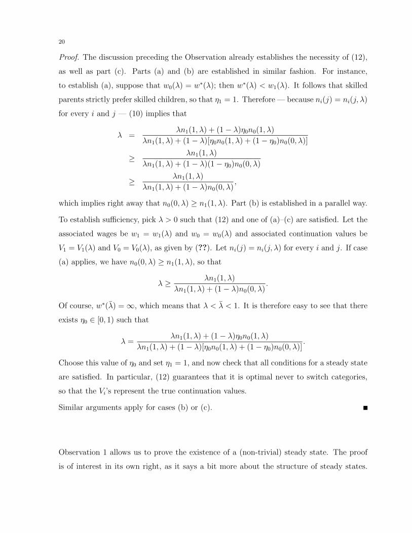
Proof. The discussion preceding the Observation already establishes the necessity of (12),

as well as part (c). Parts (a) and (b) are established in similar fashion. For instance,

to establish (a), suppose that w0(λ) = w∗(λ); then w∗(λ) < w1(λ). It follows that skilled

parents strictly prefer skilled children, so that η1 = 1. Therefore — because ni(j) = ni(j,λ)

for every i and j — (10) implies that

λ =λn1(1,λ) + (1− λ)η0n0(1,λ)

λn1(1,λ) + (1− λ)[η0n0(1,λ) + (1− η0)n0(0,λ)]

≥ λn1(1,λ)

λn1(1,λ) + (1− λ)(1− η0)n0(0,λ)

≥ λn1(1,λ)

λn1(1,λ) + (1− λ)n0(0,λ),

which implies right away that n0(0,λ) ≥ n1(1,λ). Part (b) is established in a parallel way.

To establish sufficiency, pick λ > 0 such that (12) and one of (a)–(c) are satisfied. Let the

associated wages be w1 = w1(λ) and w0 = w0(λ) and associated continuation values be

V1 = V1(λ) and V0 = V0(λ), as given by (??). Let ni(j) = ni(j,λ) for every i and j. If case

(a) applies, we have n0(0,λ) ≥ n1(1,λ), so that

λ ≥ λn1(1,λ)

λn1(1,λ) + (1− λ)n0(0,λ).

Of course, w∗(λ) = ∞, which means that λ < λ < 1. It is therefore easy to see that there

exists η0 ∈ [0, 1) such that

λ =λn1(1,λ) + (1− λ)η0n0(1,λ)

λn1(1,λ) + (1− λ)[η0n0(1,λ) + (1− η0)n0(0,λ)].

Choose this value of η0 and set η1 = 1, and now check that all conditions for a steady state

are satisfied. In particular, (12) guarantees that it is optimal never to switch categories,

so that the Vi’s represent the true continuation values.

Similar arguments apply for cases (b) or (c).

Observation 1 allows us to prove the existence of a (non-trivial) steady state. The proof

is of interest in its own right, as it says a bit more about the structure of steady states.

21

To ensure that the steady state has positive output and skill ratio, however we need to

impose the assumption of positive fixed costs of child-rearing.23

Proposition 6. There exists a steady state with λ > 0, provided r0(0) > 0 .

Proof. We display λ > 0 such that (12) and one of the conditions in (a)–(c) of Observation

1 is met. Observe that V1(λ) is decreasing and continuous in λ, while V0(λ) is increasing

and continuous in λ. It is easy to conclude that w∗(λ) is continuous in λ (in the extended

reals) and that it is strictly increasing as long as it is finite.24

On the other hand, w1(λ) is continuous and decreasing in λ, with the assumed end-point

conditions.

We must conclude that there exists (unique) λ1 > 0 such that w1(λ1) = w∗(λ1). If at this

value, n1(1,λ1) ≥ n0(0,λ1), we are done (use part (b) of Observation 1).

Otherwise n1(1,λ1) < n0(0,λ1). It is obvious that n1(1,λ) is bounded away from 0 as

λ → 0 (both parental income and V1(λ) go to infinity). On the other hand, given that

r0(0) > 0, it must be that n0(0,λ) → 0. It is easy to see that, moreover, that ni(i,λ) is

continuous for i = 0, 1. It follows that there exists a largest value of λ smaller than λ1 —

call it λ2 — such that n1(1,λ2) ≥ n0(0,λ2).

Indeed, by continuity of ni(i,λ), we must have n1(1,λ2) = n0(0,λ2). Also, w∗(λ2) ≤

w1(λ2).25 If w0(λ2) ≤ w∗(λ2) as well, then we are again done (use part (c) of Observation

1).

Otherwise w0(λ2) > w∗(λ2). Define λ3 to be the smallest value of λ > λ2 such that

w0(λ3) = w∗(λ3). It is obvious that λ3 ∈ (λ2,λ1).26 We claim that n1(1,λ3) < n0(0,λ3).

This follows right away from our definition of λ2 as the largest value of λ smaller than λ1,

23In the absence of such fixed costs, a steady state exists but may involve zero output and skill ratio.Whether an interior steady state can be shown to exist in the absence of this assumption remains an openquestion.24That is, w∗(λ) is increasing and continuous whenever it is finite, w(λ�) = ∞ if λ� > λ and w∗(λ) = ∞,and w∗(λn) → ∞ if λn → λ and w∗(λ) = ∞.25After all, w1(λ1) = w∗(λ1), the former function is declining in λ, the latter increasing in λ, and λ2 < λ1.26After all, at λ1 we have w∗(λ1) = w1(λ1) > w0(λ1), the strict inequality following from the fact thatw∗(λ1) is finite.

22

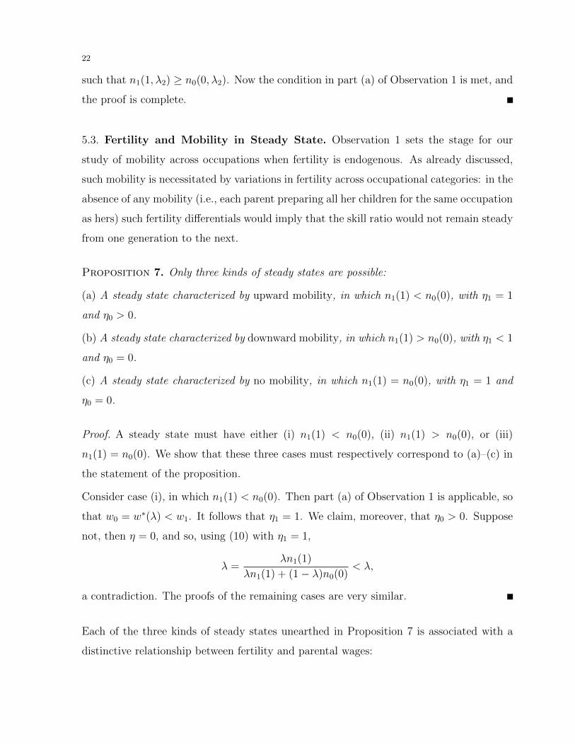
such that n1(1,λ2) ≥ n0(0,λ2). Now the condition in part (a) of Observation 1 is met, and

the proof is complete.

5.3. Fertility and Mobility in Steady State. Observation 1 sets the stage for our

study of mobility across occupations when fertility is endogenous. As already discussed,

such mobility is necessitated by variations in fertility across occupational categories: in the

absence of any mobility (i.e., each parent preparing all her children for the same occupation

as hers) such fertility differentials would imply that the skill ratio would not remain steady

from one generation to the next.

Proposition 7. Only three kinds of steady states are possible:

(a) A steady state characterized by upward mobility, in which n1(1) < n0(0), with η1 = 1

and η0 > 0.

(b) A steady state characterized by downward mobility, in which n1(1) > n0(0), with η1 < 1

and η0 = 0.

(c) A steady state characterized by no mobility, in which n1(1) = n0(0), with η1 = 1 and

η0 = 0.

Proof. A steady state must have either (i) n1(1) < n0(0), (ii) n1(1) > n0(0), or (iii)

n1(1) = n0(0). We show that these three cases must respectively correspond to (a)–(c) in

the statement of the proposition.

Consider case (i), in which n1(1) < n0(0). Then part (a) of Observation 1 is applicable, so

that w0 = w∗(λ) < w1. It follows that η1 = 1. We claim, moreover, that η0 > 0. Suppose

not, then η = 0, and so, using (10) with η1 = 1,

λ =λn1(1)

λn1(1) + (1− λ)n0(0)< λ,

a contradiction. The proofs of the remaining cases are very similar.

Each of the three kinds of steady states unearthed in Proposition 7 is associated with a

distinctive relationship between fertility and parental wages:

23

Proposition 8. A steady state with upward mobility must involve declining average fer-

tility over equilibrium wealths; that is,

(13) η1n1(1) + (1− η1)n1(0) < η0n0(1) + (1− η0)n0(0).

Exactly the opposite is true of a steady state with downward mobility, while fertility is

unchanged over equilibrium wealths for a steady state with zero mobility.

Proof. We prove the proposition for steady states with upward mobility; the other parts

can be established in very similar ways.

Consider a steady state with upward mobility. By Proposition 7, part (a), we have η1 = 1

and η0 > 0, so we need to show that

(14) n1(1) < η0n0(1) + (1− η0)n0(0).

Using (10) with η1 = 1, we have that

λ =λn1(1) + (1− λ)η0n0(1)

λn1(1) + (1− λ)[η0n0(1) + (1− η0)n0(0)]

>λn1(1)

λn1(1) + (1− λ)[η0n0(1) + (1− η0)n0(0)],

where the inequality uses the facts that λ ∈ (0, 1), η0 > 0, and ni(j) > 0 for all i and j.

Cross-multiplying and transposing terms, we see that

λ(1− λ)[η0n0(1) + (1− η0)n0(0)] > λ(1− λ)n1(1)

which establishes (14), and completes the proof.

24

This proposition establishes a precise connection between the different kinds of steady

states and fertility movements across the cross-section of observed incomes.27 These mo-

bility patterns are of interest per se, because they arise in a model with no stochastic

shocks to ability or incomes. The key to such patterns in our model is endogenously

varying fertility across income (and occupational) categories.

While downward mobility from skilled to unskilled occupations are relatively rare and per-

haps explained by bad luck, upward mobility in the reverse direction is usually considered

a reflection of determined investments made by the poor and accordingly are held as an

indication of equality of opportunity in the society in question. So it may be of interest to

provide an equilibrium explanation of this that does not rely on “luck”.28

The connection between upward mobility and declining fertility over the cross-section of

parental wages is of particular interest. Both phenomena are empirically plausible, while

sustained downward mobility (or increasing fertility on the cross-section) are not. It is

therefore useful to know that the model ties the two phenomena closely together.

To go further, we need to ask the question: to what extent can steady states with downward

or zero mobility be ruled out by the theory? We turn to this issue next.

6. The General Equilibrium of Fertility Decline

A steady state generates two observations along the parental cross-section of wages, corre-

sponding to parents in the skilled and unskilled categories. The question is: does fertility

decline as we move from the lower-income to higher-income categories, or equivalently —

by part (a) of Proposition 6 — from unskilled to skilled categories? This is what we refer

27It should be noted that this connection is not made in the earlier Proposition 7. That proposition states,for instance, that in a steady state with upward mobility, we have n1(1) < n0(0), but while the first ofthese terms is indeed the average fertility among skilled parents in such a steady state, the second of theseterms is not. The reason is that in a steady state with upward mobility, a fraction η0 of unskilled parentsdo have skilled children, so that the average fertility among unskilled parents is really

η0n0(1) + (1− η0)n0(0),

and it is this expression that needs to be compared with n1(1), which we do in (14).28To be sure, this is not the only explanation. One can derive a general theory of (nonstochastic) mo-bility by taking recourse to any factor that creates “unbalanced” intertemporal changes in steady state.Differential fertility is one such factor. One might think of others, such as nonhomothetic preferences orskill-biased technical change.

25

to as the “general equilibrium effect”. It incorporates not only parental fertility responses,

but also the endogeneity of incomes in steady state. That endogeneity places bounds on

the traditional “preference-based” effect relative to the “occupational-shift” effect.

Notice that in either category, fertility is not necessarily the same across parents; it will

vary with the occupational choice that those parents make. Recall that average fertility in

category i is

ηini(1) + (1− ηi)ni(0),

where ηi(1) is the fraction of parents from category i who put their children into the skilled

category 1, with attendant fertility ni(1), and 1−ηi(1) is the remaining fraction who choose

the unskilled category for their children, with attendant fertility ni(0).

For our result, we specialize to the case of constant-elasticity utility functions. Most

existing literature on endogenous fertility restricts attention to this class anyway. Thus

write:

u(c) =c1−ρ

1− ρ,

where ρ is positive but not equal to 1, this last restriction ensuring that we are always in

either the positive or the negative utility case. As before, accompanying restrictions need

to be placed on θ: it must have the same sign as 1− ρ.

6.1. Main Result. We provide conditions under which the occupational-shift effect in-

variably dominates the traditional preference-based determinants of fertility choice, so that

average fertility declines with income:

Proposition 9. Assume that utility is isoelastic and that childrearing and educational

functions satisfy [R.1]–[R.3]. Suppose, in addition, that at least one of the following three

conditions hold:

(a) We are in the positive utility case (0 < 1− ρ < 1) with 0 < θ ≤ 1− ρ.

(b) We are in the negative utility case (1− ρ < 0) with 0 > θ ≥ 1− ρ.

26

(c) The cost structure is separable, and involves time-costs alone; child-rearing costs take

the form k(w) = kw.

Then all steady states must involve lower average fertility in the higher occupational cat-

egory. Equivalently, by Proposition 8, every steady state must exhibit upward mobility.

Before proceeding to a formal proof, some discussion of this result will be useful.

While conditions (a)–(c) do not cover all the possible cases under isoelastic utility, Propo-

sition 9 exhibits a broad range of parameter values for which steady states must involve

upward mobility. Range (a) covers a region where the result is perhaps to be expected,

in which substitution effects associated with parental wage increases are large relative to

wealth effects. That ensures that the “traditional” effect of wage increases on fertility

(keeping child quality constant) is negative. This is reinforced by the “occupational shift”

or child quality effect to imply that unskilled households must have higher fertility, thereby

necessitating upward mobility in every steady state.

More surprising are parts (b) and (c), which allow wealth effects to outweigh substitution

effects to imply that the “traditional” wage effect on fertility is positive, as highlighted

by condition (7) of Proposition 5. Under the conditions of our proposition, these are

outweighed by the occupational-switch effect. The size of the traditional effect depends on

the wage differential between skilled and unskilled households, unlike the occupational shift

effect. The parameter assumptions in parts (b) and (c) ensure that the wage differentials

are not large enough for the traditional effect to dominate. Here the general equilibrium of

occupational choice predicts a net fertility decline over observed wages. This is perhaps one

of the few cases in which general equilibrium considerations remove ambiguities present

under partial equilibrium, instead of adding to them.

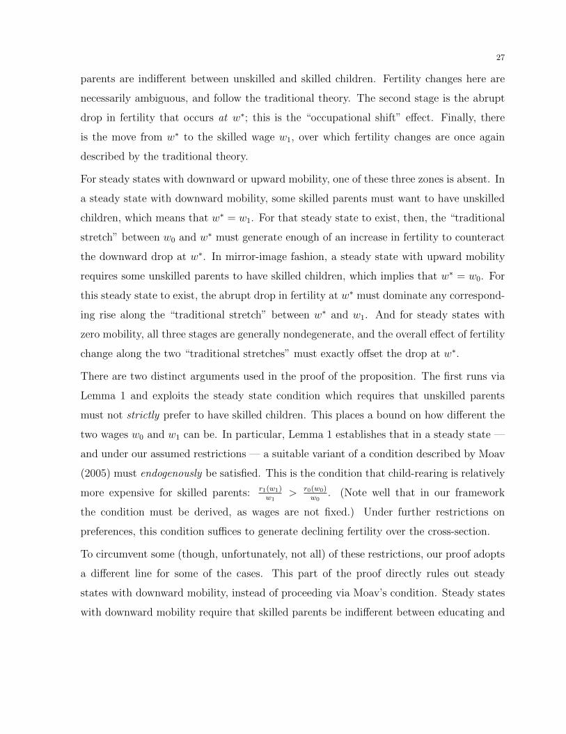
To elaborate further, consider any steady state, with wages w0 and w1. Even though

none of the intermediate wages are observed in this deterministic model, compare fertility

by mentally “moving” parental wages from w0 to w1 over three (artificial) stages. First,

move from w0, at which unskilled children are preferred, to the threshold w∗ at which

27

parents are indifferent between unskilled and skilled children. Fertility changes here are

necessarily ambiguous, and follow the traditional theory. The second stage is the abrupt

drop in fertility that occurs at w∗; this is the “occupational shift” effect. Finally, there

is the move from w∗ to the skilled wage w1, over which fertility changes are once again

described by the traditional theory.

For steady states with downward or upward mobility, one of these three zones is absent. In

a steady state with downward mobility, some skilled parents must want to have unskilled

children, which means that w∗ = w1. For that steady state to exist, then, the “traditional

stretch” between w0 and w∗ must generate enough of an increase in fertility to counteract

the downward drop at w∗. In mirror-image fashion, a steady state with upward mobility

requires some unskilled parents to have skilled children, which implies that w∗ = w0. For

this steady state to exist, the abrupt drop in fertility at w∗ must dominate any correspond-

ing rise along the “traditional stretch” between w∗ and w1. And for steady states with

zero mobility, all three stages are generally nondegenerate, and the overall effect of fertility

change along the two “traditional stretches” must exactly offset the drop at w∗.

There are two distinct arguments used in the proof of the proposition. The first runs via

Lemma 1 and exploits the steady state condition which requires that unskilled parents

must not strictly prefer to have skilled children. This places a bound on how different the

two wages w0 and w1 can be. In particular, Lemma 1 establishes that in a steady state —

and under our assumed restrictions — a suitable variant of a condition described by Moav

(2005) must endogenously be satisfied. This is the condition that child-rearing is relatively

more expensive for skilled parents: r1(w1)w1

> r0(w0)w0

. (Note well that in our framework

the condition must be derived, as wages are not fixed.) Under further restrictions on

preferences, this condition suffices to generate declining fertility over the cross-section.

To circumvent some (though, unfortunately, not all) of these restrictions, our proof adopts

a different line for some of the cases. This part of the proof directly rules out steady

states with downward mobility, instead of proceeding via Moav’s condition. Steady states

with downward mobility require that skilled parents be indifferent between educating and

28

not educating their children, and this goes towards establishing a different bound on wage

ratios, and consequently a complementary and different line of proof.29

The question arises whether Proposition 9 extends to both the positive and negative utility

models free of charge. Based on our intensive but fruitless search for a counterexample,

we tentatively conjecture that the answer to this question is in the affirmative.

6.2. Proof of Proposition 9. For ease of notation, denote n0(0) by n0 and n1(1) by n1.

We use the following

Lemma 1. Suppose that at least one of the conditions in Proposition 9 holds. Then in any

steady state,

(15)w1

r1(w1)<

w0

r0(w0).

Proof. Suppose that (15) is false in some steady state. Then w1 − r1(w1)n0 ≥ 0,30 and so,

because n1 is an optimal choice at parental wage w1,

V1 =[w1 − r1(w1)n1]1−ρ

1− ρ+ δnθ

1V1 ≥[w1 − r1(w1)n0]1−ρ

1− ρ+ δnθ

0V1.

It follows that

(16) V1 ≥[w1 − r1(w1)n0]1−ρ

(1− ρ)(1− δnθ0)

≥�r1(w1)

r0(w0)

�1−ρ [w0 − r0(w0)n0]1−ρ

(1− ρ)(1− δnθ0)

=

�r1(w1)

r0(w0)

�1−ρ

V0.

Now consider a parent with wage w0. Suppose that she chooses a fertility of n, where

(17) nr1(w0) = n0r0(w0),

29It should be noted that these parametric restrictions are typically not considered in the traditionaltheory; see, e.g., Barro and Becker (1988, page 483) and Jones and Schoonbroodt (2009, Assumptions AIand AII). The usual grounds for ruling these cases out is that second-order conditions for maximizationmay not hold. Our arguments do not rely on any second-order conditions and we therefore do not imposethese restrictions. Indeed, the appropriate second-order condition is always met; see footnote 19.30Because w0 − r0(w0)n0 ≥ 0, we have w0

r0(w0)≥ n0. Now use the negation of (15).

29

and educates all her children. Then her overall payoff is given by

V0 ≡ [w0 − r1(w0)n]1−ρ

1− ρ+ δnθV1(18)

≥ [w0 − r1(w0)n]1−ρ

1− ρ+ δnθ

�r1(w1)

r0(w0)

�1−ρ

V0(19)

=[w0 − r0(w0)n0]1−ρ

1− ρ+ δn0

θ

�r0(w0)

r1(w0)

�θ �r1(w1)

r0(w0)

�1−ρ

V0,(20)

where the first inequality follows from (16), and the last equality from (17).

Now, if there is positive utility and 1− ρ ≥ θ, as assumed, then

(21)

�r0(w0)

r1(w0)

�θ �r1(w1)

r0(w0)

�1−ρ

≥�r0(w0)

r1(w0)

�1−ρ �r1(w1)

r0(w0)

�1−ρ

=

�r1(w1)

r1(w0)

�1−ρ

> 1,

where the first inequality uses (R.2), and the last inequality uses (R.1).

On the other hand, if there is negative utility and 1− ρ ≤ θ, as assumed, then

(22)

�r0(w0)

r1(w0)

�θ �r1(w1)

r0(w0)

�1−ρ

≤�r0(w0)

r1(w0)

�1−ρ �r1(w1)

r0(w0)

�1−ρ

=

�r1(w1)

r1(w0)

�1−ρ

≤ 1,

where (R.1) and (R.2) are used again at exactly the same points.

Noting that V0 > 0 in the positive utility case and V0 < 0 in the negative utility case, we

can use (21) or (22) in equation (20) (depending on the case we are in) to conclude that

V0 >[w0 − r0(w0)n0]1−ρ

1− ρ+ δn0

θV0 = V0,

which violates part (b) of Proposition 6 for a steady state.

Finally, if condition (c) of Proposition 9 holds, (15) is obtained free of charge. For

w1

r1(w1)=

w1

kw1 + x(w1)<

1

k=

w0

r0(w0).

30

Now we turn to the main proof. The two first-order conditions for the choice of n0 and n1

tell us that

u�(c0)r0(w0)n1−θ0 =

θδu(c0)

1− δnθ0

and u�(c1)r1(w1)n1−θ1 =

θδu(c1)

1− δnθ1

.

Using the constant elasticity specification, these equalities imply that

(23)1− ρ

θ

r0(w0)

c0=

δnθ−10

1− δnθ0

and1− ρ

θ

r1(w1)

c1=

δnθ−11

1− δnθ1

,

and combining,

(24)c1c0

=r1(w1)n

θ−10 (1− δnθ

1)

r0(w0)nθ−11 (1− δnθ

0).

If there is a steady state with zero mobility, so that n0 = n1, then (24) immediately implies

thatw1 − r1(w1)n1

r1(w1)n1=

c1r1(w1)n1

=c0

r0(w0)n0=

w0 − r0(w0)n0

r0(w0)n0,

and using n0 = n1 once again, we must conclude that

w1

r1(w1)=

w0

r0(w0),

which contradicts the assertion (15) of Lemma 1.

We now eliminate steady states with downward mobility. The following lemma completes

part of this task:

Lemma 2. If ρ+ θ ≥ 1 in the positive utility case, and without any further assumptions in

the negative utility case, ni and wi/ri(wi) must co-move over the two occupations i = 0, 1.

Proof. Recall (23). Define α ≡ (1 − ρ)/θ (always a positive number) and µi ≡ wi/ri(wi)

for i = 0, 1. Then (23) can be written as

(25) δ(α− 1)nθi + δµin

θ−1i = α

for i = 0, 1. The left hand side of this expression is strictly increasing in µi. By using a

standard argument, we establish the co-movement of ni and µi if we can show that the

31

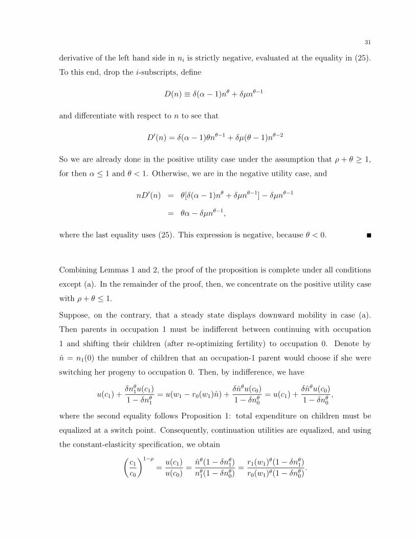
derivative of the left hand side in ni is strictly negative, evaluated at the equality in (25).

To this end, drop the i-subscripts, define

D(n) ≡ δ(α− 1)nθ + δµnθ−1

and differentiate with respect to n to see that

D�(n) = δ(α− 1)θnθ−1 + δµ(θ − 1)nθ−2

So we are already done in the positive utility case under the assumption that ρ + θ ≥ 1,

for then α ≤ 1 and θ < 1. Otherwise, we are in the negative utility case, and

nD�(n) = θ[δ(α− 1)nθ + δµnθ−1]− δµnθ−1

= θα− δµnθ−1,

where the last equality uses (25). This expression is negative, because θ < 0.

Combining Lemmas 1 and 2, the proof of the proposition is complete under all conditions

except (a). In the remainder of the proof, then, we concentrate on the positive utility case

with ρ+ θ ≤ 1.

Suppose, on the contrary, that a steady state displays downward mobility in case (a).

Then parents in occupation 1 must be indifferent between continuing with occupation

1 and shifting their children (after re-optimizing fertility) to occupation 0. Denote by

n = n1(0) the number of children that an occupation-1 parent would choose if she were

switching her progeny to occupation 0. Then, by indifference, we have

u(c1) +δnθ

1u(c1)

1− δnθ1

= u(w1 − r0(w1)n) +δnθu(c0)

1− δnθ0

= u(c1) +δnθu(c0)

1− δnθ0

,

where the second equality follows Proposition 1: total expenditure on children must be

equalized at a switch point. Consequently, continuation utilities are equalized, and using

the constant-elasticity specification, we obtain

�c1c0

�1−ρ

=u(c1)

u(c0)=

nθ(1− δnθ1)

nθ1(1− δnθ

0)=

r1(w1)θ(1− δnθ1)

r0(w1)θ(1− δnθ0).

32

Combining this equation with (24), we see that

r1(w1)nθ−10 (1− δnθ

1)

r0(w0)nθ−11 (1− δnθ

0)=

r1(w1)θ/(1−ρ)(1− δnθ1)

1/(1−ρ)

r0(w1)θ/(1−ρ)(1− δnθ0)

1/(1−ρ),

or

(26)r1(w1)r0(w1)θ/(1−ρ)

r0(w0)r1(w1)θ/(1−ρ)=

n1−θ0 (1− δnθ

1)ρ/(1−ρ)

n1−θ1 (1− δnθ

0)ρ/(1−ρ)

.

Because our steady state has downward mobility, we have n1 > n0, which implies that the

right-hand side of (26) is strictly smaller than 1 under condition (a).

On the other hand, the left hand side is given by

r1(w1)r0(w1)θ/(1−ρ)

r0(w0)r1(w1)θ/(1−ρ)=

r1(w1)(1−θ−ρ)/(1−ρ)r0(w1)θ/(1−ρ)

r0(w0)≥ 1,

given the assumptions of the Proposition as well as (R.1) and (R.2). This contradiction

completes the proof.

7. Steady State Determinacy and Comparative Statics

7.1. Local Determinacy. We now turn to the question of local determinacy of steady

states. Local determinacy permits us to derive the effects of changed policies, but is

of substantive intrinsic interest as well. It bounds the extent of hysteresis or history-

dependence that the model permits. In contrast, most models of occupational choice with

a discrete set of occupations and exogenous fertility are characterized by a continuum of

steady states. We show that incorporation of endogenous fertility into the model eliminates

this indeterminacy.

The intuitive basis for this finding is that steady states with either upward or downward

mobility can no longer be associated with strict incentives for members of both occupations:

at least one occupation must be indifferent between preparing their children for the same

occupation and switching to the alternative occupation. This indifference ties down the

steady state skill ratio and per-capita income. And if a steady state involves no mobility,

it requires equality of fertility decisions across the two occupations, which also ties down

relative wages and hence the equilibrium skill ratio.

33

To show this formally, introduce a parameter ν of the costs of educating children, and

suppose that costs of children prepared for the unskilled occupation r0(w) is independent

of ν, while the costs of children r1(w; ν) trained for the skilled occupation is strictly (and

smoothly) increasing in ν.

Proposition 10. Skill ratios forming a steady state with upward or downward mobility

are locally unique and finite in number, for a set of parameter values ν of full Lebesgue

measure. The same is true for steady states with zero mobility, provided θ is positive.

Proof. Recall the characterization of steady states in Observation 1: a steady state with

downward mobility satisfies w∗(λ) = w1(λ) and with upward mobility satisfies w∗(λ) =

w0(λ). So for either of these kinds of steady states, it suffices to show (via standard

transversality arguments, e.g., see Mas-Colell, Whinston and Green (1995, Proposition

17.D.3)) that an increase in educational cost parameter ν causes w∗(λ) to strictly increase,

for any λ.

Note initially that at any given λ, V0 is unchanged, while V1 must fall as ν rises. This

follows from the fact that in steady state it is optimal for unskilled parents to not educate

their children, so they must be unaffected by the rise in ν. And it is optimal for skilled

people to educate their children, so they must be worse off when ν rises.

Next, manipulate the first order condition (2) for fertility decisions for occupation i to

obtain the following equivalent version:

(27) rθi u�(wi − Ei)Ei = δEθ

i .θVi

where Ei ≡ ri(wi)n(wi, i) denotes total expenditure on children who are trained for the

same occupation, and all variables are evaluated at the given skill ratio. It is evident that

all decisions of unskilled parents are unaffected.

Consider first the case where θ is positive. Then θV1 falls as ν rises. So (2) implies that

fertility n1 of skilled parents must fall (where ni ≡ n(wi, i)). Now observe that (27) can

also be written as

(28) u�(wi − Ei)Ei = δnθi .θVi

34

Since n1 and θV1 both fall, it follows from (28) that E1 must fall. Since θ > 0, and E0 is

unaffected, it follows that parents are less inclined to educate their children (as they tend

to maximize child expenditures), and w∗ must rise.

Now suppose θ < 0. In this case θV1 rises as ν rises. Equation (27) now implies that

E1 rises. Since parents make human capital decisions for their children on the basis of

minimization of total expenditures, they are again less inclined to educate their children,

and w∗ must rise.

Since the wage functions wi(λ) are unaffected by the change in ν, the result now follows for

steady states with either upward or downward mobility. Steady states with zero mobility

must satisfy the condition that n(w1(λ), 1) − n(w0(λ), 0) = 0, and an increase in ν must

cause the left-hand-side of this equation to fall when θ is positive (n1 must fall while n0 is

unaffected, from (2)).

7.2. Long Run Comparative Statics. We now explore the long run effects of varying

costs of child-rearing and of education, as well as regulations pertaining to child labor

and redistributive tax-transfer policies. It will be helpful to restrict attention to a linear

formulation of child-rearing cost:

(29) r0(w) = f + k.w, r1(w) = f + k.w + x

where f denotes the fixed ‘goods cost’ incurred per child, k the parental time away from

work, and x a fixed cost of education.

Moreover, we focus attention on steady states with upward mobility, i.e., on the cases

covered by Proposition 9. Note that both functions w∗(λ), w0(λ) are increasing in λ. w∗

tends to a negative number as λ tends to 0, and to ∞ as λ tends to λ. At the same time

w0 tends to 0 and w(λ) respectively. Hence there exists at least one skill ratio where w∗

and w0 are equalized, where the w∗ curve cuts the w0 from below (i.e., has a steeper slope).

If n0 > n1, call this a locally stable steady state with downward mobility. Intuitively, if

λ falls slightly below the steady state, w∗ is smaller than w0. Then both unskilled and

skilled households would want to educate their children so the skill ratio will tend to rise.

35

Conversely, if λ rises slightly above the steady state, w∗ would be higher than w0, thus

eliminating the willingness of some unskilled households to educate their children, and the

skill ratio will fall.

The linear formulation of child rearing costs allows us to obtain a closed form expression

for the threshold wage:

(30) w∗(λ) =1

k[x{(V1(λ)

V0(λ))1θ − 1}−1 − f ]

from the first-order conditions for fertility choice.31 The threshold wage depends on the

skill ratio via the dependence of the wage in occupation i and continuation values Vi on

this ratio:

(31) Vi(λ) =u(wi(λ)− ni(wi(λ))(f + kwi(λ) + xi))

1− δni(wi(λ))θ

where in addition ni(wi) denotes the optimal fertility choice of a parent with wage wi and

selecting the same occupation for her children.

Specifically, small perturbations in child-rearing cost parameters f, x can be shown to be

shift the w∗ function (and hence the steady state skill ratio) in opposite directions, provided

we impose an additional mild assumption on preferences in the case of negative utility):

Proposition 11. In the case of negative utility, assume in addition to [U1]–[U4] that u�

−u

is decreasing.32 Consider any steady state skill ratio with upward mobility which is locally

stable. A small increase (resp. decrease) in fixed cost component f of child-rearing (resp.

education cost x) will cause the steady state skill ratio to fall (resp. rise).

Proof. Given expression (30) for w∗, it suffices to show that the derivative of V1(λ)V0(λ)

with

respect to f and x are respectively positive and negative in the case where θ > 0 (and

signs reversed in the case that θ < 0), at any steady state with upward mobility.

31Using E to denote total expenditures ((rw + f + xi)n) on children, the first order condition impliesE1−θU �(w − E) = [ 1

rw+f+xi ]θVi for occupation choice i = 0, 1. This generates condition (30).

32This condition is satisfied by constant elasticity utility functions, as well as u(c) = −exp(−ac) witha > 0.

36

Recall that

(32) Vi(λ) = maxni

[u(wi(λ)− (rwi(λ) + f + xi)ni) + δnθiVi(λ)].

Applying the Envelope Theorem to this optimization problem we have

(33)∂Vi(λ)

∂f= −u�(ci(λ))ni(λ)

1− δni(λ)θ

where ni(λ) denotes the optimal choice of ni, and ci(λ) ≡ wi(λ)− (kwi(λ) + f + xi)ni(λ).

Therefore

(34) V0(λ)∂V1(λ))

∂f− V1(λ)

∂V0(λ))

∂f= −V0(λ)

u�(c1(λ))n1(λ)

1− δn1(λ)θ+ V1(λ)

u�(c0(λ))n0(λ)

1− δn0(λ)θ.

Next, note that in any steady state with upward mobility we have n1 < n0, which in turn

implies that c1 > c0 (in order to ensure that V1 > V0).

In the case of positive utility where θ > 0, it follows that expression (34) is positive.

In the case of negative utility where θ < 0, use expression (32) for the value function to

see that expression (34) reduces to

(35)u(c1)

1− δnθ1

u�(c0)n0

1− δnθ0

− u(c0)

1− δnθ0

u�(c1)n1

1− δnθ1

Since n0 > n1, it suffices that [−u(c1)].u�(c0) ≥ [−u(c0)].u�(c1) for (35) to be negative. This

is ensured by the property that u�

−u is non-increasing.

It follows that ∂w∗

∂f < 0.

A simpler argument ensures that ∂w∗

∂x > 0. The argument is simpler because the V0 function

is locally unaffected by a small rise in x, while ∂V1∂x = −u�(c1)n1

1−δnθ1

< 0.

Hence the w∗ curve shifts down following an increase in f or a decrease in x, while the

position of the w0(λ) is not affected. If the steady state is locally stable, a small rise in f

or fall in x must cause the skill ratio to rise.

The model thus allows for local determinacy and comparative statics of long-run effects of

changes in key parameters of the child-raising technology. This is in contrast to both the

37

Barro-Becker theory (which lacks credit market imperfections) as well as most preceding

models of occupational choice (which lack endogenous fertility).

The comparative static results follow from the effect of the parametric changes on parental

incentives to invest in the education of their children. A rise in the ‘goods cost’ of child-

rearing increases this incentive, just as a fall in education costs does. The former induces

a reduction in fertility, which in turn stimulates an increase in desired quality of children.

This is for both a direct reason (child-care expenses per child are lower when not investing

in education, so a rise in f raises child-care costs by more for non-investors) and an indirect

reason (the continuation utility of skilled children falls by less than for unskilled children).

It predicts that societies with a norm where extended family or kinship networks share

the burden of child-rearing (so the parents bear a smaller part of the burden) will tend

to invest less in education of children. Social changes that cause a shift from joint to

nuclear families thus induce higher education. Policies of subsidized childcare undermine

skill accumulation incentives, and raise inequality between skilled and unskilled wages.

Effects on aggregate fertility are ambiguous. Consider the case of positive utility. A rise

in f tends to lower fertility among both skilled and unskilled households at any given skill

ratio.33 This is further reinforced by the induced rise in the proportion of skilled households,

since the skilled tend to have fewer children. If wealth effects dominate substitution effects,

there is a counteracting effect: fertility within unskilled households rise as a consequence of

the rise in the skill ratio.34 So the net effect on the fertility of the unskilled is ambiguous,

while fertility among the skilled must fall. Since the effects on the fertility differential

between skilled and unskilled are ambiguous, so are the effects on mobility. It is therefore

possible that lower education costs actually end up lowering mobility, if wages and fertility

among the unskilled rise sufficiently. This provides a potential explanation for the empirical

33This is both because of the direct effect of rising child-rearing costs, as well as the induced reductionof continuation values of skilled and unskilled (since θ > 0 in the case of positive utility. If utility werenegative, θ < 0, and the falling continuation values would induce higher fertility. So the ambiguity is evenmore pronounced with negative utility.34If the substitution effects dominate instead, fertility among the skilled will rise as a consequence ofthe fall in their wages. And fertility among the unskilled will fall as their wages rise. In this case thefertility differential will widen, implying a rise in mobility. But the effects on aggregate inequality remainambiguous.

38

findings of Chechhi, Ichino and Rustichini (1999) that mobility in Italy appears to be lower

than in the US, despite a more extensive public schooling system and a lower skill premium

in wages.

7.3. Child Labor. Now suppose children that do not go to school can work and augment

the incomes of their households. Suppose that children can work as a substitute for un-

skilled adult labor, and earn a wage of γw0, where γ ∈ (0, 1) is a parameter that reflects

differences in work capacity between adults and children, as well as regulations concern-

ing child labor. Stronger restrictions on child work correspond to a reduction in γ. The

preceding model pertains to the case where γ = 0.

Household consumption corresponding to parental wage w is now c ≡ w − [rw + f + xi−

γw0(1 − i)]n. This corresponds to our earlier model if we replace f by f � ≡ f − γw0 and

x by x� ≡ x+ γw0. To ensure f � > 0 we must impose the restriction that γ < fw0(λ)

.

Stronger restrictions on child labor then correspond to a fall in γ, which is analytically

equivalent to a rise in child care costs combined with a fall in education cost. Proposition

prcompstat then implies that both of these induce a rise in the long run steady state skill

ratio.

There is an additional effect that operates through the effect on wages (stressed in partic-

ular by Basu and Van (1998)): a reduction in child labor reduces the supply of unskilled

labor in the economy as a whole, which tends to raise unskilled wages. Hence the w0(λ)

curve shifts up. This has an additional effect on a steady state with upward mobility, since

it is characterized by intersection of the w∗ curve and the w0 curve. If the steady state is

locally stable, this effect raises the steady state skill ratio even further.

Hence the net effect of stronger regulations on child labor is to raise the ‘level’ of long run

development: higher per capita skill and income, with lower wage inequality between the

skilled and unskilled. Effects on aggregate fertility and mobility are, however, ambiguous

for the reasons explained above.

7.4. Income Redistribution via Taxes and Transfers. We now show that the results

obtained in Mookherjee and Ray (2008) with regard to the effect of different tax-transfer

39

schemes in the occupational choice model with exogenous fertility continue to extend. In

their setting there was some arbitrariness associated with selection of a particular skill

ratio from the continuum of steady state skill ratios. As shown above this arbitrariness

disappears with endogenous fertility.

We provide a brief outline of the analysis here, omitting most details. Consider first an

unconditional welfare system paying an income support of σ to unskilled households, which

are financed by income taxes levied on skilled households at a constant linear rate τ . In

steady state, budget balance requires (1−λ)σ = λτw1(λ), so the size of the income support

depends on the skill ratio and tax rate:

(36) σ =λ

1− λτw1(λ)

Steady states have similar properties as established in preceding sections, except that the

values of being unskilled and skilled are now given by

(37) V0 = maxn0

[u(w0 + σ − (kw0 + f)n0) + δnθ0V0]

(38) V1 = maxn1

[u((1− τ)w1 − (kw1(1− τ) + f + x)n1) + δnθ1V1].

These policies lower the value of being skilled, and raise the value of being unskilled.

Investment in education is thereby discouraged: the w∗ curve shifts up.35 The long run

effect will be to lower per capita skill in the economy. This will raise the skill premium in

wages, so the market will undo some of the redistribution.36

The adverse long-run effects of unconditional income supports to the poor can be avoided

with conditional transfers. An example is an education subsidy which is funded by income

taxes on the skilled. In this case the continuation value of the unskilled is not directly

affected: the value can be computed on the basis of the assumption that they do not invest

35In this case the thresholds differ between skilled and unskilled parents. What matters, of course, in asteady state with upward mobility is the threshold for unskilled parents, and it is this threshold that werefer to here.36Implications for fertility are complex. The wealth effects associated with the transfers will tend to raisefertility among the unskilled and lower them among the skilled. Countering this in the opposite directionare the effects of wage movements induced by the policies, since unskilled wages fall and skilled wages rise.

40

in education of their children, whence they receive no benefits from the transfers. On the

other hand, the continuation value of being skilled rises, since skilled households have more

options.37 This encourages investment in education: the w∗ curve shifts down, and the

steady state skill ratio rises (hence so does per capita income, while the skill premium

declines). The effects are exactly the opposite of an unconditional welfare system.

7.5. Gender Discrimination and Family Planning Subsidies. One can extend the

model to allow for two parents of differing genders who allocate their time between child-

rearing and working outside the home on a labor market. The effects of policies encouraging

female labor force participation or reducing gender discrimination on the labor market turn

out to be ambiguous, as their effect is similar to a rise in the time cost k of children on

parental human capital investment incentives.38

The effect of family planning subsidies is similar to a combination of a lump-sum income

subsidy, and a rise in f , the incremental goods cost of higher fertility. The latter promotes

investment incentives as we have seen above. If the subsidies are funded by lump-sum

taxes, there are no wealth effects, and the net effect is the same as an increase in f alone,

i.e., a rise in per capita income and skill.

8. Relationship to the Literature

We start by describing related literature on the wage-fertility correlation.

First, as discussed in the Introduction, there is the view that the cross-sectional relation-

ship is indeed positive, and the negative relationship we do in fact see is the result of

some omitted variable. Becker (1960) is a proponent of this point of view, emphasizing the

possible differences between desired and actual numbers of children, owing to ignorance

37An education subsidy π lowers private education cost to x−π. Hence budget balance requires τw1(λ) =n1(λ)π, i.e., skilled households pay the taxes to fund the education subsidies they would avail if they chosethe same fertility as in the absence of the subsidy. In that case they are as well off as before. But theyhave the option to have a different number of children, which could make them better off.38The direct effect of an increase in k is similar to that of f : both raise w∗, enhancing skill investmentincentives. The indirect effect is difficult to assess. In the positive utility case for instance, it is no longerclear that a rise in k raises V1

V0, as this effect is proportional to the wage rate which is higher for the skilled.

41

concerning contraceptive methods. Another important omitted variable (see, e.g., Freed-

man (1963)) is that family income is correlated with greater female participation in the

labor force, and it is the latter that drives the decline. (This view can, of course, be folded

into the substitution effect which is driven by time costs of rearing children.) Under this

view, then, theory has little to say about the net effect.

Second, there is the view that the cross-sectional relationship is “truly” negative, and

must be explained by the theory at hand. Attempts include appropriate calibration of the

parameters, so that substitution effects kill off the income effect, introduction of ‘quality’

of children as an additional choice coupled with suitable assumptions concerning child-

rearing costs (Becker and Lewis (1973), Becker and Tomes (1976), Moav (2005))), or

the introduction of non-homotheticities in preferences (see, e.g. Galor and Weil (2000),

Greenwood and Seshadri (2002), or Fernandez, Guner and Knowles (2005)).

Jones, Schoonbroodt and Tertilt (2008) provide an overview of these explanations, and

argue that they all require restrictive assumptions. Instead they suggest an argument that

relies on heterogeneity in parental tastes. Parents who want larger families will realize that

more time will be spent on bringing up children, and this lowers their optimal choice of

human capital, not for their children as in our framework, but for themselves. Therefore

larger families would tend to have lower incomes.

Steady state models with endogenous fertility, in which the cross-sectional relationship

is explicitly addressed, include Alvarez (1999) and Kremer and Chen (1999, 2002). Al-

varez introduces Barro-Becker preferences into Loury’s (1981) theory of intergenerational

inequality. The main objective is to see how the persistence result in inequality (arising

from shocks) withstands endogenous fertility, but as a byproduct Alvarez obtains the re-

sult that fertility is positively correlated with parental wealth.39 In a modification of the

model, Alvarez introduces various non-separabilities in preferences and rearing costs; in

particular, increasing marginal costs in child-rearing. If these effects are strong enough, this

baseline finding may be reversed. In summary, the model delivers the opposite result on

39In fact, in his baseline model, the positive correlation is so strong that per-child parental transfers areindependent of parental wealth.

42

fertility-wealth in its baseline setup and an ambiguous prediction when the modifications

are introduced.

Kremer and Chen use a special specification of parental preferences, in which utility is

given by c + log n. Parents must spend time in child-rearing, but do not care about the

quality of children or the payoffs enjoyed by them. This assumed absence of income effects

implies that rising parental wages exert only substitution effects on the demand for fertility.

Hence fertility is decreasing in parental wages. In this sense, the Kremer-Chen exercise

is a special case of the parametric calibration that forces substitution effects to dominate

income effects.

The same is true of Doepke (2004), who assumes that utility functions exhibit lower cur-

vature than the log function, and that there are no goods costs involved in child-rearing.

In this case, as we have seen in Proposition 5, wealth effects are weaker than substitution

effects, ensuring a negative wage-fertility correlation.

Our Proposition 9 is clearly very different from all of the preceding explanations of the

wage-fertility correlation, as it does not rest on assumed weakness of wealth effects or

unobserved preference heterogeneity, but instead on the endogeneity of occupational wages

and related steady state restrictions.

Some of our partial equilibrium findings, which serve as the preliminaries leading up to

Proposition 9, are related to results in Doepke (2004). While Doepke considers the positive

utility case alone and does not address the general equilibrium finding of Proposition 9, his

Proposition 3 implies the jump-down as occupational boundaries are crossed (derived for

a more restrictive class of preferences and rearing/schooling costs). Doepke’s Proposition

4 makes the point that in equilibrium, there could be upward, downward or zero mobility

outcomes, and also observes that in the first two cases the parents in the “out-migrating”

category will need to be indifferent between educating and not educating their children.

Doepke subsequently expresses the view that the first of these three outcomes is the most

relevant one, though without providing any theoretical justification, and then moves on

to calibration and empirical investigation. Our contribution is to provide a theoretical

justification for the focus on this class of steady states. An added contribution are the

43

theoretical results concerning local determinacy and comparative static properties of steady

states.

Finally, we discuss the connections to the occupational choice literature. The generic model

of occupational choice with fixed fertility40 takes as given a set of occupations (typically

two, as in the exercise here). The steady-state conditions are simple: no dynasty currently

in one occupation must wish to move their progeny to another with a different setup cost.

This occupational persistence follows from single-crossing, which rules out cycles in oc-

cupational choice. In particular, there is no mobility in steady state. Such a model can

generate intergenerational mobility by adding to it stochastic shocks in ability or income

(as in Banerjee and Newman (1993) or Mookherjee and Napel (2007)). Our theory as-

cribes, however, a predictable direction to mobility; it occurs (even without any stochastic

shocks) to compensate for the endogenous fertility differentials between skilled and un-

skilled households. The local isolation of steady states in our theory permits tractable

comparative statics analysis, with the absence of stochastic shocks greatly simplifying the

analysis.

9. Concluding Remarks

We have developed a theory on the implications of interactions between fertility and hu-

man capital in a setting with imperfect financial markets. This framework provides new

insights into the wage-fertility relationship, the determinants of intergenerational mobility,

and the extent of macroeconomic history dependence. It provides a tractable framework

permitting comparative static analysis of effects of changes in a variety of fiscal and human

capital policies. It also illustrates a number of possible factors underlying observed fea-

tures of the demographic transition in developing countries, whereby economic and social

factors associated with urbanization and modernization induce large declines in fertility

40Versions of this model appear in Banerjee and Newman (1993), Ljunqvist (1993), Galor and Zeira(1993), Ghatak and Jiang (2002), and Mookherjee and Ray (2003). Ray (1990, 2006) contains a modelwhich exactly aligns with this generic description in the two-occupation case.

44

(e.g., falling costs of education, rising costs of childcare, regulations on child labor). Un-

derlying all of these is an induced shift towards occupations requiring higher investments

in education.

A number of gaps in our results still remain, which we hope can be filled by future re-

search. One concerns the generality of the finding that steady states with downward or

zero mobility do not exist. Others include the existence of interior steady states in the case

of zero fixed costs of childcare, and local determinacy of steady states without mobility in

the case of negative utility.

An obvious next step would be to subject the findings of this paper to empirical testing.

The central finding of this paper is that the occupational shift effect accounts for a ro-

bust negative correlation between parental wages and fertility, which may work against a

positive wealth effect. Hence within occupations or human capital categories, or in con-

texts where there is not much scope for occupational or human capital variations, the

wage-fertility correlation may be positive. Similarly over short periods of time when occu-

pations of the adult population are unchanging, fertility may move in the same direction

as income. But the correlation across occupational categories will typically be negative.

These are consistent with empirical findings reported in some earlier literature such as

Freedman (1963) and Simon (1969), and it would be interesting to see if they continue to

be confirmed more broadly using more powerful econometric techniques and other datasets

(e.g. pertaining to developing countries).

References

Aghion P. and Bolton P. (1997). ”A Theory of Trickle-Down Growth and Develop-

ment.” Review of Economic Studies, 64, 151-172.

Alvarez, F. (1999), “Social Mobility: The Barro-Becker Children Meet the Laitner-Loury

Dynasties,” Review of Economic Dynamics 2, 65–103.

Bandyopadhyay D. (1997). “Distribution of Human Capital and Economic Growth,”

Working Paper no. 173, Department of Economics, Auckland Business School.

45

Banerjee, A. and Newman, A. (1993). “Occupational Choice and the Process of

Development.” Journal of Political Economy 101, 274–298.

Barro, R. and G. Becker (1989), “Fertility Choice in a Model of Economic Growth,’

Econometrica 57, 481–501.

Basu K. and P. Van (1998), “The Economics of Child Labor,” American Economic

Review, 88(3), pp. 412-27.

Becker, G. (1960), “An Economic Analysis of Fertility,” in Demographic and Economic

Change in Developed Countries, Princeton: Princeton University Press.

Becker, G. and R. Barro (1986), “Altruism and the Economic Theory of Fertility,”

Population and Development Review 12, Supplement Issue, 69–76.

Becker, G. and R. Barro (1988), “A Reformulation of the Economic Theory of Fer-

tility,” Quarterly Journal of Economics 103, 1–25.

Becker G. and H.G. Lewis(1973), “On the Interaction between the Quantity and

Quality of Children,” Journal of Political Economy, 81(2), S279-S288.

Becker G. and N. Tomes (1976), “Child Endowments and the Quantity and Quality

of Children,” Journal of Political Economy, 84(4), Part 2, S143-S162.

Becker G. and Tomes, N. (1979), “An Equilibrium Theory of the Distribution of

Income and Intergenerational Mobility,” Journal of Political Economy, 87(6), 1153–89.

Becker, G., Murphy, K. and R. Tamura (1990), “Human Capital, Fertility and

Economic Growth,” Journal of Political Economy 98, S12–S37.

Blau, D., and W. van der Klaauw (2007), “The Impact of Social and Economic

Policy on the Family Structure Experiences of Children in the United States,” mimeo,

Department of Economics and Carolina Population Center, University of North Carolina.

Borg, M. O. (1989), “The IncomeFertility Relationship: Effect of the Net Price of a

Child,” Demography, 26, 301-310.

Caucutt, E. M., N. Guner and J. Knowles (2002), “Why Do Women Wait? Match-

ing, Wage Inequality and the Incentive for Fertility Delay,” Review of Economic Dynamics,

5, 815-855.

46

Checchi A., A. Ichino and A. Rustichini (1999), “More Equal but less Mobile?

Education Financing and Intergenerational Mobility in Italy and in the U.S.,” Journal of

Public Economics, 74, 351-393.

Cho, L.-J. (1968), “Income and Differentials in Current Fertility,” Demography, 5, 198211.

Clark, G. (2005), “Human Capital, Fertility, and the Industrial Revolution,” Journal of

the European Economic Association, 3, 505515.

Clark, G. (2007), Farewell to Alms: A Brief Economic History of the World, Princeton

University Press.

Clark, G. and G. Hamilton (2006), “Survival of the Richest: The Malthusian Mech-

anism in Pre-Industrial England,” Journal of Economic History, 66, 707736.

Dahan, M. and D. Tsiddon (1998), “Demographic Transition, Income Distribution and

Economic Growth,” Journal of Economic Growth 3, 29–52.

De La Croix, D. and M. Doepke (2003), “Inequality and Growth: Why Differential

Fertility Matters,” American Economic Review 93, 1091–1113.

Docquier, F. (2004), “Income Distribution, Non-Convexities and the Fertility-Income

Relationship,” Economica 71, 261–273.

Doepke, M. (2004), “Accounting for Fertility Decline During the Transition to Growth,”

Journal of Economic Growth 9, 347–383.

Doepke, M. (2005), “Child Mortality and Fertility Decline: Does the Barro-Becker Model

Fit the Facts?,” Journal of Population Economics 18, 337–366.

Easterlin, R. (1973), “Relative Economic Status and the American Fertility Swings,”

in Family Economic Behavior, Eleanor B. Sheldon (ed.) (Philadelphia, PA: Lippincott).

Fernandez, R., Guner, N. and J. Knowles (2005), “Love and Money: A Theoret-

ical and Empirical Analysis of Household Sorting and Inequality,” Quarterly Journal of

Economics 120, 273–344.

Fleischer, B. M. and G. Rhodes (1979), “Fertility, Womens Wage Rates, and Labor

Supply,” American Economic Review, 69, 1424.

47

Freedman, D. S. and A. Thorton (1982), “Income and Fertility: The Elusive Rela-

tionship,” Demography, 19, 6578.

Freedman, D. (1963), “The Relation of Economic Status to Fertility,” American Eco-

nomic Review 53, 414–426.

Freeman, S. (1996), “Equilibrium Income Inequality among Identical Agents.” Journal

of Political Economy 104, 1047–1064.

Galor, O. and Zeira, J. (1993), “Income Distribution and Macroeconomics.” Review

of Economic Studies 60, 35–52.

Galor, O and D. Weil (2000), “Population, Technology, and Growth: FromMalthusian

Stagnation to the Demographic Transition and Beyond,” American Economic Review 90,

806–828.

Ghatak, M. and N. Jiang (2002), “A Simple Model of Inequality, Occupational Choice

and Development” Journal of Development Economics 69, 205–226.

Greenwood, J. and A. Seshadri (2002), “The U.S. Demographic Transition,” Amer-

ican Economic Review (Papers and Proceedings) 92, 153–159.

Haines, M. R. (1976), “ Population and Economic Change in Nineteenth Century Eastern

Europe: Prussian Upper Silesia, 1840-1913,” The Journal of Economic History, 36, 334358.

Heckman, J. J. and J. R. Walker (1990), “ The Relationship between Wages and the

Timing and Spacing of Births: Evidence from Swedish Longitudinal Data,” Econometrica,

58, 14111441.

Jones, L. and A. Schoonbroodt (2009),“Complements versus Substitutes and Trends

in Fertility Choice in Dynamic Models,” forthcoming, International Economic Review.

Jones, L., Schoonbroodt, A. and M. Tertilt (2008), “Fertility Theories: Can They

Explain the Negative Fertility-Income Relationship?” mimeo., Department of Economics,

University of Minnesota.

Jones, L. and M. Tertilt (2008): “An Economic History of Fertility in the United

States: 1826–1960,” in Frontiers of Family Economics, P. Rupert (ed.), Vol. 1, Emerald

Press, 165–230.

48

Kremer, M. and L. Chen (1999), “Income Distribution Dynamics with Endogenous

Fertility,” American Economic Review 89, 155–160.

Kremer, M. and L. Chen (2002), “Income Distribution Dynamics with Endogenous

Fertility,” Journal of Economic Growth 7, 227–258.

Lee, R. (1987), “Population Dynamics of Humans and Other Animals,” Demography, 24,

443466, Presidential Address to the Population Association of America.

Ljungqvist, L. (1993), “Economic Underdevelopment: The Case of Missing Market for

Human Capital,” Journal of Development Economics 40, 219–239.

Lloyd-Ellis, H. and Bernhardt D. (2000), “Enterprise, Inequality and Economic

Development,” Review of Economic Studies 67, 147–168.

Loury, G. (1981), “Intergenerational Transfers and the Distribution of Earnings.” Econo-

metrica July 1981, 49(4), pp. 843–867.

Mas-Colell A., Whinston M. and Green J. (1995), Microeconomic Theory, New

York: Oxford University Press.

Matsuyama, K. (2000), “Endogenous Inequality”, Review of Economic Studies 67, 743–

759.

Matsuyama, K. (2006), “The 2005 Lawrence Klein Lecture: Emergent Class Structure,”

International Economic Review 47, 327–260.

Merrigan, P. and Y. S. Pierre (1998), “An Econometric and Neoclassical Analysis

of the Timing and Spacing of Births in Canada from 1950-1990,” Journal of Population

Economics, 11, 2951.

Moav O.(2005), “Cheap Children and the Persistence of Poverty,” Economic Journal,

115(500), 88-110.

Mookherjee D. and Napel S. (2007), “Intergenerational Mobility and Macroeconomic

History Dependence,” Journal of Economic Theory.

Mookherjee, D. and D. Ray (2002), “Is Equality Stable?,” American Economic Review

92 (Papers and Proceedings), 253–259.

49

Mookherjee, D. and D. Ray (2003), “Persistent Inequality,” Review of Economic

Studies 70, 369–394.

Mookherjee, D. and D. Ray (2008), “A Dynamic Incentive-Based Argument for Con-

ditional Transfers,’ Economic Record, September 2008, 84, S2-16.

Ray, D. (1990), “Income Distribution and Macroeconomic Behavior,”. Mimeo, Boston

University.

Ray, D. (2006), “On the Dynamics of Inequality,” Economic Theory 29, 291–306.

Sah, R. (1991), “The Effects of Child Mortality Changes on Fertility Choice and Parental

Welfare,” Journal of Political Economy 99, 582–606.

Schultz, T. P. (1986), “The Value and Allocation of Time in High-Income Countries:

Implications for Fertility,” Population and Development Review, 12, 87108.

Shiue, C. H. (2008), “ Human Capital and Fertility in Chinese Clans, 1300-1850,” mimeo,

Department of Economics, University of Colorado at Boulder.

Simon, J.L. (1969), “The Effect of Income on Fertility,” Population Studies, 23(3), 327–

341.

Simon, J. L. (1977), The Economics of Population Growth, Princeton, New Jersey.

Spengler, J. (1952), “Population Theory,” in A survey of Contemporary Economics,

Vol. 2, B. Haley (Ed.), Homewood.

Westoff, C. F. (1954), “Differential Fertility in the United States: 1900 to 1952,”

American Sociological Review 19, 549–561.

Whelpton P.K. and C.V. Kiser (1951), Social and Psychological Factors Affecting

Fertility, Milbank Memorial Fund, Vol 1–4.

Wrigley, E. A. (1961), Industrial Growth and Population Change. Cambridge Univer-

sity Press, Cambridge.