UNIVERSITY OF HUDDERSFIELD
Integrated Tactile-Optical Coordinate
Measurement for the Reverse Engineering
of Complex Geometry
by
FENG LI
A thesis submitted in partial fulfilment for the
degree of Doctor of Philosophy
in the
School of Computing and Engineering
Centre for Precision Technologies
November 2014
i
Copyright Statement The author of this thesis (including any appendices and/or schedules to this thesis)
owns any copyright in it (the “Copyright”) and s/he has given The University of
Huddersfield the right to use such copyright for any administrative, promotional,
educational and/or teaching purposes.
Copies of this thesis, either in full or in extracts, may be made only in accordance
with the regulations of the University Library. Details of these regulations may be
obtained from the Librarian. This page must form part of any such copies made.
The ownership of any patents, designs, trademarks and any and all other intellectual
property rights except for the Copyright (the “Intellectual Property Rights”) and any
reproductions of copyright works, for example graphs and tables (“Reproductions”),
which may be described in this thesis, may not be owned by the author and may be
owned by third parties. Such Intellectual Property Rights and Reproductions cannot
and must not be made available for use without the prior written permission of the
owner(s) of the relevant Intellectual Property Rights and/or Reproductions.
ii
Abstract
Complex design specifications and tighter tolerances are increasingly required in modern
engineering applications, either for functional or aesthetic demands. Multiple sensors are
therefore exploited to achieve both holistic measurement information and improved reliability
or reduced uncertainty of measurement data. Multi-sensor integration systems can combine
data from several information sources (sensors) into a common representational format in
order that the measurement evaluation can benefit from all available sensor information and
data. This means a multi-sensor system is able to provide more efficient solutions and better
performances than a single sensor based system. This thesis develops a compensation
approach for reverse engineering applications based on the hybrid tactile-optical multi-sensor
system.
In the multi-sensor integration system, each individual sensor should be configured to its
optimum for satisfactory measurement results. All the data measured from different
equipment have to be precisely integrated into a common coordinate system. To solve this
problem, this thesis proposes an accurate and flexible method to unify the coordinates of
optical and tactile sensors for reverse engineering. A sphere-plate artefact with nine spheres is
created and a set of routines are developed for data integration of a multi-sensor system.
Experimental results prove that this novel centroid approach is more accurate than the
traditional method. Thus, data sampled by different measuring devices, irrespective of their
location can be accurately unified.
This thesis describes a competitive integration for reverse engineering applications where the
point cloud data scanned by the fast optical sensor is compensated and corrected by the
slower, but more accurate tactile probe measurement to improve its overall accuracy. A new
competitive approach for rapid and accurate reverse engineering of geometric features from
multi-sensor systems based on a geometric algebra approach is proposed and a set of
programs based on the MATLAB platform has been generated for the verification of the
proposed method. After data fusion, the measurement efficiency is improved 90% in
comparison to the tactile method and the accuracy of the reconstructed geometric model is
improved from 45 micrometres to 7 micrometres in comparison to the optical method, which
are validated by case study.
iii
Acknowledgements
This thesis was written while studying in the ECMPG (Engineering Control and Machine
Performance Group) of the University of Huddersfield. I am very grateful to both for their
generosity and financial support. Without their support I would have been unable to write this
thesis and present myself as a PhD candidate.
Firstly and foremost, I would like to express my great acknowledgements to my main
supervisor Dr. Andrew P. Longstaff for his committed supervision throughout the entire
duration. His profound knowledge and experiences guide my works under the correct
direction. And his respectable personality also makes me feel pleasure during the three years
when I stayed in ECMPG.
I would also address my unstinting appreciations to my second and third supervisors: Dr.
Simon Fletcher and Professor Alan Myers. Each has provided valuable input, both
professional and personal.
Additionally, thanks to all the members in ECMPG. They gave me their sincere assistance
which made me feel comfortable during the periods I spent in ECMPG.
Finally, I prefer to give my heartfelt appreciations to my parents and my other relatives.
Thanks for their selfless support and encouragements in this difficult journey.
iv
Contents
Copyright Statement i
Abstract ii
Acknowledge iii
List of Figures viii
List of Tables x
Abbreviations xi
Chapter 1: Introduction ............................................................................................................. 1
1.1. Introduction .................................................................................................................... 2
1.2. Motivation & scope ........................................................................................................ 2
1.3. Aims & objectives .......................................................................................................... 4
1.4. Outline ............................................................................................................................ 5
Chapter 2: Multi-sensor Integration in Dimensional Measurement .......................................... 7
2.1. Introduction .................................................................................................................... 8
2.2. Sensor techniques for coordinate measurement ............................................................. 8
2.2.1. Tactile probing......................................................................................................... 9
2.2.1.1. Principle of the tactile probing system ............................................................. 9
2.2.1.2. Modelling of the tactile probing system ......................................................... 11
2.2.1.3. Calibration of the tactile probing system ........................................................ 13
v
2.2.2. Laser scanning ....................................................................................................... 13
2.2.2.1. Principle of the laser scanning system ............................................................ 13
2.2.2.2. Modelling of the laser scanning system ......................................................... 15
2.2.2.3. Calibration of the laser scanning system ........................................................ 18
2.2.3. Fringe projection ................................................................................................... 19
2.2.3.1. Principle of fringe projection system .............................................................. 19
2.2.3.2. Modelling of fringe projection system ........................................................... 20
2.2.3.3. Fringe image processing ................................................................................. 23
2.2.4. Comparison of the three sensors ............................................................................ 26
2.3. Multi-sensor integration in coordinate measurement ................................................... 26
2.3.1. Multi-sensor configuration .................................................................................... 27
2.3.2. Theoretical aspects of multi-sensor data fusion..................................................... 28
2.3.2.1. Data pre-processing ........................................................................................ 29
2.3.2.2. Data registration ............................................................................................. 29
2.3.2.3. Data fusion...................................................................................................... 30
2.3.3. Related research in multi-sensor integration ......................................................... 30
2.3.3.1. Homogeneous optical sensors integration ...................................................... 31
2.3.3.2. Inhomogeneous optical sensors integration .................................................... 32
2.3.3.3. Tactile and optical multi-sensor integration ................................................... 32
2.3.3.4. Other multi-sensor integration ........................................................................ 35
2.3.3.5. Commercial multi-sensor systems .................................................................. 36
2.3.3.6. Data format conversion for the system integration in CAD/CAM environment
..................................................................................................................................... 36
2.4. Summary ...................................................................................................................... 37
Chapter 3: Coordinate Unification for Integrated Tactile-Optical Systems ............................ 38
3.1. Introduction .................................................................................................................. 39
3.2. Geometric transform method for hybrid system unification ........................................ 40
3.3. Calibration board design............................................................................................... 40
3.4. Hybrid system configuration and calibration ............................................................... 41
vi
3.4.1. Elements of the hybrid system............................................................................... 41
3.4.2. Hybrid system calibration ...................................................................................... 42
3.5. Proposed method and algorithm description ................................................................ 43
3.5.1. Proposed method ................................................................................................... 43
3.5.2. Mathematical model of 3D Cartesian coordinate transformation .......................... 43
3.5.3. The principle of non-linear least squares ............................................................... 44
3.6. Experiment results and error analysis ........................................................................... 47
3.6.1. Coordinate unification of the CMM and structured light system .......................... 48
3.6.2. Coordinate unification of CMM and FaroArm laser scanner ................................ 49
3.7. Summary ...................................................................................................................... 51
Chapter 4: Reverse Engineering of Geometry Based on Multi-sensor System ....................... 52
4.1. Introduction .................................................................................................................. 53
4.2. Discrete Geometry Processing in Reverse Engineering ............................................... 53
4.2.1. Point data pre-processing ...................................................................................... 55
4.2.2. Multi-view data registration .................................................................................. 56
4.2.3. Polyhedral surface generation ............................................................................... 57
4.2.4. Shape recognition and segmentation ..................................................................... 57
4.2.5. Model Reconstruction ........................................................................................... 58
4.2.5.1. Surface representations ................................................................................... 59
4.2.5.2. Boundary representation (B-rep) model creation ........................................... 61
4.2.5.3. Blend reconstruction and further beautification ............................................. 62
4.2.6. Reverse Engineering of sample workpiece ........................................................... 63
4.3. Best-fit and compensation for geometric elements based on multi-sensor system ...... 64
4.3.1. Related works in competitive multi-sensor integration ......................................... 64
4.3.2. Least squares best fit geometric elements ............................................................. 65
4.3.2.1. Optimization algorithm .................................................................................. 66
4.3.2.2. Least squares best fit plane ............................................................................. 68
4.3.2.3. Least squares sphere ....................................................................................... 69
4.3.2.4. Gauss-Newton strategy for cylinders and cones ............................................. 71
vii
4.3.2.5. Least squares cylinder .................................................................................... 73
4.2.3.6. Least squares cone .......................................................................................... 75
4.3.3. Description of the proposed method ...................................................................... 78
4.3.3.1. Proposed method ............................................................................................ 78
4.3.3.2. Algorithms description ................................................................................... 80
4.4. Summary ...................................................................................................................... 83
Chapter 5: Experimental Implementation ............................................................................... 85
5.1. Multi-sensor system configuration ............................................................................... 86
5.1.1. System overview ................................................................................................... 86
5.1.2. Sensors description ................................................................................................ 87
5.2. Case study one: simple geometric shapes..................................................................... 89
5.3. Case study two: plane-sphere-cylinder-cone ................................................................ 92
5.4. Case study three: complex housing .............................................................................. 96
5.4.1. Multi-data acquisition ............................................................................................ 96
5.4.2. Discrete geometry processing and CAD model reconstruction ............................. 98
5.4.2.1. Point data segmentation and compensation .................................................... 98
5.4.2.2. Triangle mesh generation and shape recognition ........................................... 98
5.4.2.3. Model Reconstruction .................................................................................... 99
5.4.3. Measurement speed and accuracy comparison ...................................................... 99
5.4.3.1. Measurement speed comparison for sensors .................................................. 99
5.4.3.2. CAD model accuracy comparison ................................................................ 100
5.4.4. Further improvement of the reconstructed model ............................................... 101
5.5. Summary .................................................................................................................... 104
Chapter 6: Conclusions & Future Work ................................................................................ 105
6.1. Summary .................................................................................................................... 106
6.2. Contributions of this thesis ......................................................................................... 108
6.3. Future work ................................................................................................................ 108
References ............................................................................................................................. 110
viii
List of Figures
Figure 2-1: Existing sensor techniques for measurement .......................................................... 8
Figure 2-2: Typical resulition and measuring range plots for optical sensors and tactile probes
in coordinate measuring systems ............................................................................................... 9
Figure 2-3: Limitations of the tactile probing system ............................................................. 10
Figure 2-4: Probing system in coordinate measurement ......................................................... 12
Figure 2-5: Triangulation principles in laser scanning ............................................................ 14
Figure 2-6: Perspective projection model of the laser line scanning system ........................... 16
Figure 2-7: FPP scanning process ........................................................................................... 20
Figure 2-8: FPP system model ................................................................................................ 21
Figure 2-9: Typical calibration patterns .................................................................................. 25
Figure 2-10: Sensors configurations in multi-sensor systems ................................................. 28
Figure 3-1: Spheres calibration board ..................................................................................... 41
Figure 3-2: Elements of the integrated system ........................................................................ 42
Figure 3-3: Spheres surface and centres measured from tactile and optical systems .............. 47
Figure 4-1: Flowchart for a RE workpiece .............................................................................. 54
Figure 4-2: Three commonly used data filtering methods ...................................................... 55
Figure 4-3: RE of a sample part .............................................................................................. 64
Figure 4-4: Points data translation and rotation....................................................................... 72
Figure 4-5: Cone fitting ........................................................................................................... 77
Figure 4-6: Schematic of the proposed method ....................................................................... 79
Figure 4-7: New flowchart of RE by using hybrid contact-optical measuring system............ 80
Figure 4-8: Flowchart of plane compensation by using multi-sensor measuring system ........ 81
Figure 4-9: Flowchart of sphere compensation by using multi-sensor measuring system ...... 82
ix
Figure 4-10: Flowchart of cylinder compensation by using multi-sensor measuring system . 83
Figure 4-11: Flowchart of cone compensation by using multi-sensor measuring system ....... 84
Figure 5-1: Nikon LK V 15.10.8 HA high accuracy ceramic bridge CMM ........................... 86
Figure 5-2: Fitting results of sphere using different methods.................................................. 90
Figure 5-3: Fitting results of cylinder using different methods ............................................... 91
Figure 5-4: Standard deviations of fitting results of different methods................................... 91
Figure 5-5: Points data measured using multi-sensor system .................................................. 92
Figure 5-6: Point cloud data segmentation .............................................................................. 93
Figure 5-7: Mesh surface ......................................................................................................... 95
Figure 5-8: Tested workpiece and sensor selection ................................................................. 96
Figure 5-9: Examples of the acquired data .............................................................................. 98
Figure 5-10: Points cloud data after segmentation .................................................................. 98
Figure 5-11: Points cloud data after segmentation .................................................................. 99
Figure 5-12: CAD model reconstruction ................................................................................. 99
Figure 5-13: The comparison of geometric features ............................................................. 102
Figure 5-14: The comparison of geometric features & freeform .......................................... 103
x
List of Tables
Table 2-1: Comparison of the main characteristics of the three sensors ................................. 26
Table 3-1: The components of the integrated system .............................................................. 42
Table 3-2: The standard deviation on the centre and the radius of the spheres ....................... 47
Table 3-3: The coordinates of sphere centres .......................................................................... 48
Table 3-4: The coordinates of the centroids ............................................................................ 48
Table 3-5: The residuals & RMSR of coordinates (CMM & structured light) ....................... 49
Table 3-6: The residuals & RMSR of coordinates (CMM & FaroArm laser) ......................... 50
Table 5-1: Nikon LK V 15.10.8 HA high accuracy ceramic bridge CMM ............................. 87
Table 5-2: Specifications of the Renishaw SP25M scanning probe system ............................ 87
Table 5-3: Specifications of the Nikon LC15Dx laser scanner ............................................... 88
Table 5-4: Comparison of the tactile probe and the laser sensor ............................................. 89
Table 5-5: Fitting results using different methods (Dimensions in mm) ................................. 94
Table 5-6: Computational time ................................................................................................ 94
Table 5-7: Numbers of points and scanning time .................................................................... 97
Table 5-8: The residuals & RMSR of coordinates (Zeiss & Nikon LC15Dx) ...................... 100
Table 5-9: RMS comparison ................................................................................................. 101
xi
Abbreviations
B-Splines Basis Splines
CAD Computer-Aided Design
CAM Computer-Aided Manufacturing
CCD Charge-Coupled Device
CMM Coordinate Measuring Machine
CNC Computer Numerical Control
CT Computed Tomography
DLP Digital Light Processing
FE Forward Engineering
FPP Fringe Projection Profilometry
ICP Iterative Closest Point
IGES Initial Graphics Exchange Specification
ISO International Standards Organisation
MPEE Maximum Permissible Error for Length Measurement
NURBS Non Uniform Rational B-spline
PLM Product Lifecycle Management
STEP Standard for the Exchange of Product Model Data
STL Stereo Lithography or Standard Triangulation Language
RMS Root Mean Square
RMSR Root Mean Square of Residuals
RP Rapid Prototyping
2
1.1. Introduction
In many areas of industry, 3D point data measured from the surfaces of physical objects has
been widely adopted in a variety of product development processes, such as product
inspection, quality control, reverse engineering (RE), etc. In measurement applications,
different sensing technologies are available for data acquisition, such as tactile probing, laser
scanning, fringe projection, etc. It has been shown that each technique has its own
characteristics and application. Complex design specifications and tighter tolerances are
increasingly required in modern engineering applications, either for functional or aesthetic
demands. The geometric specifications embedded in these parts such as shapes and surfaces,
dimensions, geometrical tolerances, surface characteristics, surface material, etc. make it
difficult to satisfy all the measurement requirements with only one single sensor in
dimensional measurement. Multiple sensors are therefore exploited to achieve both holistic
measurement information and improved reliability or reduced uncertainty of measurement
data.
The basic motivation for multi-sensor data fusion is to improve the quality and usability of the
measurement result, e.g. in a production process. Multi-sensor integration systems can
combine data from several information sources (sensors) into a common representational
format in order that the metrological evaluation can benefit from all available sensor
information and data. This means a multi-sensor system is able to provide more efficient
solutions and better performances than the single sensor based system. This additional
metrological benefit may be termed multiple sensors synergy. Synergistic effects may
improve the performance of a multi-sensor system in at least one of the following ways:
increased spatial and temporal coverage and better resolution, increased robustness to sensor
and algorithmic uncertainty, better noise suppression and improved accuracy [1]. Particular
features of a workpiece can be measured with the most suitable sensor, and measurements
with better accuracy can be used to correct data from other sensors which exhibit relevantly
larger systematic errors but have a wider field of view or application range.
1.2. Motivation & scope
Traditionally, the development of industrial products begins with the goals expected of the
product function. Design engineers conceptualise the components required in a product, and
develop the product through the procedures of design, fabrication, inspection, and assembly.
Each procedure requires detailed design drafts or process charts. Such a developing flow is
called forward engineering (FE). In recent years, RE, the opposite of FE, has received
increasing attention. Reverse engineering refers to the process of analysing the construction of
3
a product when there are no design documents available from its original production. RE
serves many purposes including:
1) Developing a similar or improved product/design.
2) Creating adaptors or enclosures to the original product.
3) Reproducing an existing part.
Existing tactile coordinate measuring machine (CMM) methods are widely used for industrial
dimensional metrology [2], but the digitisation process on such systems is very time-
consuming for the acquisition of the initial set of points on complex or freeform surfaces if
applied to RE. Another disadvantage in the context of RE is that a predefined path must be
specified in advance to cover all features of a workpiece that are to be probed. This requires a
prior knowledge of the part, presenting an obstacle to future automatic RE strategies. An
alternative approach is represented by non-contact digitisation of surfaces based on optical
triangulation techniques [3]. Triangulation sensor usually can capture dense point clouds
efficiently in terms of speed and required human intervention. Additionally, it offers the
possibility of measuring surface points from multiple features via a single and relatively
simple probing path. Therefore it has been widely used in RE applications and quality control
methods of freeform surfaces. In general, optical methods are considered to be less accurate
in comparison with tactile probing in measurements of geometric features [4].
To meet the requirement of both high speed and high accuracy 3D measurement for RE,
multi-sensor measuring systems have been developed to measure, analyse and rebuild the
CAD model of objects. Hybrid contact-optical coordinate measuring systems are each
designed by Chan, et al. [5], Carbone, et al. [6], Shen, et al. [7] and Sladek, et al.[8] where the
obtained information digitized by an optical sensor is used to guide the touch probe for re-
measuring the sample surfaces. The presented systems are cooperative integrations where
optical sensors acquire the global shape information of objects to guide the touch probes for
automatic point sensing. They are, however, limited to dealing with workpieces with
relatively simple features.
Therefore, this thesis aims at developing an effective competitive integration approach for the
compensation of an optical scanner by using a tactile probe to perform the RE of complex
shape parts. The part should have both common geometric features and freeform surface; it
also has non-surface features, such as slots or holes. The work of this thesis mainly focuses on
three aspects: multi-sensor system integration, geometric elements modelling and fitting, and
fused data compensation.
4
In a multi-sensor integration system, each single sensor needs to be configured properly for
satisfactory measurement results. The resolution, measuring ranges and working principles of
the multiple sensors are usually different. Each individual sensor works in their own separate
coordinate system, then all the data from different coordinate systems have to be precisely
integrated into a common source.
An integrated multi-sensor system results in a variety of information and data. They require a
unified and consistent data representation. Standard file formats provide an effective way to
represent the data and exchanged with other systems in coordinate measurement. The parts
measured by multi-sensor system usually comprise complex surfaces and features. Multi-
sensor data fusion requires suitable methods and algorithms to process the multiple data
acquired from different sensors. The methods in the RE of geometry include: data registration,
polyhedral surface generation, shape recognition and segmentation and model reconstruction.
The discrete shapes should be best-fitted to different geometric elements based on
mathematical and numerical principles. The integrated system accuracy and resolution depend
on all separate systems, but should be biased towards the precise tactile method. A
compensation approach for RE based on the multi-sensor integration system is developed in
this thesis.
1.3. Aims & objectives
The aim of this thesis is to propose & validate the competitive integration of inhomogeneous
sensors in the context of reverse engineering applications. The focus of this study is to
compensate inaccuracies of the point cloud data using more accurate tactile probing. The
measurement volume of workpiece discussed in this thesis ranges from 20 mm ×20 mm ×20
mm to 500 mm ×500 mm ×500 mm. The measurement speed of the hybrid system is expected
to be similar to optical method and the accuracy is close to tactile system. The main
objectives of the thesis are:
• A universal approach to unify tactile and optical sensors for the measurement of
geometric features
• A workflow based on tactile-optical multi-sensor techniques for RE applications
• A set of algorithms for discrete geometry fitting and initial estimates
• A set of programs for geometric elements best-fit and compensation of point cloud
data
5
• A fast and accurate method for RE of complex shape part based on a multi-sensor
technique, which can take advantage of the fast speed of the optical sensor & high
accuracy of the tactile probe
1.4. Outline
The thesis is organized as follows:
Chapter 2 describes three measuring techniques commonly used in dimensional measurement:
tactile probing, laser scanning and fringe projection. Their working principle and
mathematical model are discussed separately. The calibration method of each technique is
also presented. The multi-sensor configurations and data fusion procedures, as well as the
related works in multi-sensor integration for dimensional measurement are detailed.
Chapter 3 introduces a new approach, which is called the “centroid of spherical centres”
method, for tactile-optical measuring system coordinate integration. The benefits of the
proposed method are improved accuracy in coordinate unification, and the method is a
universal approach to be used to integrate a CMM touch probe and optical sensors. An
additional advantage of this method is that different measuring devices do not need to be
placed in the same workplace.
Chapter 4 first describes the common data processing methods for RE applications. The
workflow for RE mainly includes these operations: data pre-processing, data registration,
meshing, shape recognition and segmentation, and model reconstruction. Then the least
squares methods for best-fit geometric elements are presented. A synthesized initial
estimation for nonlinear functions of the least squares algorithms is discussed. Finally a
compensation method for hybrid tactile-optical system in RE application is proposed.
Chapter 5 first introduces the multi-sensor measuring platform and investigates the
measurement errors of laser line scanning by using tactile probing as a reference. The
feasibility and robustness of the proposed approach are also examined. Then a part with only
geometric features is used to evaluate the method proposed in Chapter 4 after data
segmentation. Then a detailed case study of RE of an industrial housing workpiece by using
multi-sensor competitive approach is presented. The developed programs based on the Matlab
platform are exploited to verify the proposed algorithms. Finally, the multi-sensor data
compensation, the CAD model reconstruction process, the measurement speed using different
methods and the accuracy evaluation of the studied workpiece are presented.
6
Chapter 6 summarizes the thesis with conclusions drawn from the study and propose some
promising directions for the future research.
8
2.1. Introduction
Acquiring 3D point data from physical objects is increasingly being adopted in a variety of
product development processes, such as quality control and inspection, reverse engineering
and many other industrial fields. A variety of sensor technologies have been developed to
meet the requirement of surface digitization with different accuracy and measuring ranges.
2.2. Sensor techniques for coordinate measurement
Different sensor technologies are developed for surface digitization in dimensional
measurement. According to whether the probes or sensors contact the surface, the data
acquisition methods can basically be divided into two categories: tactile measurement
methods and non-contact measurement method [9]. Figure 2-1 gives an overview of the
classification of some of the existing sensor techniques [10].
Figure 2-1: Existing sensor techniques for measurement
In this thesis, three data acquisition techniques are implemented in our experiments: tactile
probing, laser line scanning and fringe projection. These techniques have been widely used in
dimensional measurement, their typical resolution and measuring range plots are shown in
Figure 2-2 [11]. Their working principles and calibrations are discussed in the following
sections.
9
(a) Resolution (b) Measuring range
Figure 2-2: Typical resulition and measuring range plots for optical sensors and tactile probes
in coordinate measuring systems
2.2.1. Tactile probing
2.2.1.1. Principle of the tactile probing system
Tactile probing systems are usually used in cases where surface measurements allow or
require lower point data density, such as the inspection of prismatic objects, workpiece
surfaces with a known CAD model or a shape without large variation. The measuring ranges
span from sub-micrometre to several millimetres in one, two or three dimensions. In a special
case, 2.5 dimensional probing systems are planar sensitive and have only limited
sensitivity/measuring range perpendicular to this plane [11].
The tactile probing sensors are usually slower in acquiring points compared to optical sensors.
Their contact working features make them unsuitable for measuring soft material objects.
Other limitations of the probing systems are that surface zones might not be measured if the
sizes of these regions are smaller than the diameter of the tip ball or peaks might lead to the
smoothed approximation of the surface (Figure 2-3 (a)). Moreover, the different sizes of the
stylus tips also influence the measurement results as shown in Figure 2-3 (b) [2]. However,
the touch trigger probing systems are generally considered to show a higher accuracy in
comparison to optical sensors [4]. They are simple, more adaptive to the environment and not
sensitive to ambient light which greatly affect the accuracy of optical systems.
10
(a) Inaccessible regions (b) Influence of the different tip sizes
Figure 2-3: Limitations of the tactile probing system
The working principle of tactile probes is based on a mechanical interaction with the
workpiece surface and they usually measure in more than one direction. There are two
differentiated modes, touch trigger mode and scanning mode.
In the touch trigger mode, the data acquisition speed is usually slow (1~2 points/second). The
probe mechanism generates a trigger signal with the help of information obtained by a
displacement measuring system; the signal can be triggered when a certain threshold value is
exceeded. Reaction force from the probing system to the CMM must be as low as possible [2].
However, if the triggering force is too low the false triggers will be detected due to inertia.
The trigger signal generated by the probe in real time will be processed to record the position
of the contact point. Therefore, the touch trigger probing process contains two basic steps.
First a trigger signal is generated when a surface is touched by the moving tip. And then
followed by a withdrawing procedure, the signal is generated again when the tip is back off
the surface, the stylus returns to its previous position and is ready for next point probing. A
disadvantage of this method is that it may take a long time as the process of approaching the
surface and withdrawing has to be repeated for each point to be probed.
In scanning mode, the probe tip is always in contact with the surface during the scanning
process. The touching element is guided on a line along the surface while a set of coordinates
are sampled in a time sequence. The points acquired by scanning sensors (up to 500
points/second) are much more than the trigger sensors. However, as the stylus constantly and
consistently contacts the work surface, their measurement uncertainty is higher than touch
trigger probing because of dynamic measurement errors. The main difference between
scanning and touch trigger probes is that scanning probes use electrical springs and small
linear drives, which generate their probing force electronically instead of mechanically like
touch trigger probes [12]. In general, the scanning sensors are more complex in structure, data
analysis and monitor control than the touch trigger sensors. Accordingly, the scanning sensors
are suitable to perform the measurement of size, position and profile of precise geometric
11
features, while the touch trigger sensors can be exploited for shapes without significant
variations [10].
A limitation of tactile probing for RE is that prior knowledge of the part is required for
efficient data capture. This is necessary to guide the probe to touch the surface. Without such
knowledge, the probe must scan very slowly, even when not contact with the part, or else risk
damage upon collision. Very few examples exist, such as Renishaw Cyclone scanning system
that uses a ‘raster scanning’ method to digitize the surface, where this is not the case.
2.2.1.2. Modelling of the tactile probing system
Most frequently a tactile probing system is a 3D data acquisition system, which means that
the initial acquired data are 3D in ( ), , x y z coordinates. The geometrical information of
workpiece can be derived from this 3D data. Therefore, a tactile probing system has to have at
least the following features to fulfil its requirements [2]:
• A contact element to establish an interaction with the surface (e.g. tip ball, disc or
cone)
• A transmitting component to transfer information about the interaction from the
contact element to the sensor (e.g. stylus shaft)
• A force generating element (suspension) to produce a defined probing force (e.g.
spring)
• A sensor to sense the interaction between the contact element and the surface (e.g.
electric switch)
• An output transmitting the information for triggering a length measuring device (e.g.
scale) or for further processing (e.g. correction of bending, taking into account
qualified tip ball radius, evaluation in instrument’s software).
Most often, the functional characteristics of the probing systems can be derived from a
Cartesian (most coordinate measuring machines), cylindrical, or a spherical coordinate system.
The probing process requires the definition of the coordinate systems for data acquisition.
Three coordinate systems are defined in a 3D tactile probing system as shown in Figure 2-4
[2].
12
Figure 2-4: Probing system in coordinate measurement
Where Ar
is the position vector of the actual contact point A in the workpiece coordinate
system (WCS). rr
represents the position vector of the origin of the probe coordinate system
(PCS) in the machine coordinate system (MCS). Cr
stands for the position vector of the
origin of the WCS in the MCS. wr
denotes the point vector of the contact point in MCS. pr
represents the position vector of the centre of the tip ball in the PCS. And b
denotes the tip
correction vector which starts from the centre of the tip to the contact point.
From the coordinate systems relationships described in Figure 2-4, the final result of Ar
can
be derived. wr
in the MCS and WCS is represented as:
w c Ar r r= +
(2-1)
While wr
in the MCS and PCS can be represented as:
w r pr r r b= + +
(2-2)
Then we can obtain the position vector of point A:
13
A r p cr r r b r= + + −
(2-3)
2.2.1.3. Calibration of the tactile probing system
In order to perform correct measurements, the position of the tip ball centre point related to
the reference point of the probing system ( pr
in Figure 2-4) and the radius of the tip ball
(absolute value of b
in Figure 2-4) must be known first [13]. This is the main purpose of a
calibration process. There are many factors influencing these parameters, such as probing
force (magnitude and direction), pre-travel of the probe, wear of tip ball, plastic deformation,
elastic behaviour of probing system, styli, wear of workpiece surface, temperature and other
influences [2].
The parameters can be determined experimentally with a calibrated artefact under the same
conditions. This procedure is called probing system qualification. The most common used
calibrated artefact is a sphere (diameter 10 mm to 50 mm). A sphere has the advantages that it
is as very precise calibrated standard and can be positioned without regard to rotational
position. Its surface has normal vectors in every spatial direction, therefore the correction of
tip ball diameter can be independent of normal direction of surface [2]. The qualification is
developed in different strategies by each manufacturer of CMMs/probing systems because of
the very different probing systems. However, the general qualification strategy includes the
following steps [14]:
• Selection of the calibrated artefact
• Choice of the location and orientation of the artefact
• Definition of number, location and sequence of probing points (for scanning mode:
scanning lines, data rate, and travelling speed)
Each influencing parameter (probing force and direction, operating mode, stylus with tip ball
etc.) must be chosen as far as possible to be identical with the measurement to be performed
afterwards with the qualified probing system [2].With the probed points, the parameters to be
calibrated can be derived by mathematical fitting methods and then the parameters can be
exploited for compensation of acquired data from the surface.
2.2.2. Laser scanning
2.2.2.1. Principle of the laser scanning system
In comparison to tactile probing, the laser scanner can acquire a high density of point data
with significantly higher measurement speed (typically thousands to tens of thousands of
14
points per second). Laser scanning offers the possibility to measure surfaces points from
multiple features in a single scanning pass resulting in relatively simpler probing paths,
reducing the human labour required. Its non-contact nature also makes it suitable to measure
the surfaces with flexible materials [3]. This makes it a common choice in RE applications
and quality control of free form surfaces. However, laser line scanning is sensitive to issues
almost irrelevant to tactile based methods such as ambient light, surface colour, shininess,
transparency and other surface properties influencing the measurement results [15]; it also
suffers from digitizing of the non-surface features, such as slots or holes, due to occlusions
and obscuration of these artefacts.
The laser scanner works based on optical triangulation method. Within the triangulation
principle a point on an object surface can be determined by the trigonometric relations
between a camera, a projector and the object itself. A basic geometric relationship for a 1D
triangulation principle is shown in Figure 2-5 (a) [16].
(a) Triangulation in 1D (b) Triangulation in 2D
Figure 2-5: Triangulation principles in laser scanning
Where, a single camera is aligned along the z-axis with the center of the lens located at origin.
At a baseline distance b , to the left of the camera (along the negative x axis− ), a laser
projector sends out a beam of light at a variable angle θ , relative to the x axis− baseline.
The point ( ), , x y z is projected into the digitized image at the pixel ( )', 'x y so
' 'x z x f= and ' y z yf= by similar triangles, where f is the focal length of the camera
in pixels. The measured quantities ( )', ',x y θ are used to compute the ( ), , x y z coordinates:
'cos '
bx xf xθ
=−
(2-4)
15
'cos '
by yf xθ
=−
(2-5)
cos 'bz f
f xθ=
− (2-6)
For any fixed focal length f and baseline distance b , the range resolution of a triangulation
system is only limited by the ability to accurately measure the angle θ and the horizontal
position 'x .
The measuring areas of common laser triangulation sensor (1D sensor) range from
millimeters to centimeters [3]. The laser point scanning in 1D is limited in accuracy and
efficiency. An extension of the triangulation principle is known as laser line scanning (2D
sensor). The laser line scanner projects a laser plane onto the specimen and so a profile can be
captured by camera each time, as shown in Figure 2-5 (b). The calculation method of each
point on the scanning line or profile is similar as the 1D triangulation. However, the
efficiency is greatly improved.
The accuracy of a laser scanner usually depends on many factors, such as the optical
aberration of the lenses, the calibration method used, the relative position of the scanner and
the object, the view angle and the condition of the surfaces etc. [17, 18]. The typical
measurement range of laser scanning is ± 5 to ± 250 mm, and accuracy is about 1 part in
10,000 and measurement frequency of 40 kHz or higher [19, 20].
2.2.2.2. Modelling of the laser scanning system
As the laser line scanner is a 2D sensor, the camera of the scanner acquires a line image on
the CCD (charge-coupled device) camera array at each scan. Each pixel on the line image
corresponds to a point on the object surface. As the perspective projection principle is most
commonly used in camera model [21], the modelling of a laser scanning system is shown in
Figure 2-6 [22].
16
Figure 2-6: Perspective projection model of the laser line scanning system
Where CCS is 3D camera coordinates system, OC is the optical center of the camera,
Z axis− is the optical axis of the camera lens, and CO X and CO Y are parallel to AO X and
AO Y , respectively. AO XY is CCD array plane coordinates system, AO is the intersection of
the Z axis− and AO XY ,WCS is 3D workpiece coordinate system (also can be regarded as
world coordinate system), which is set up to describe the position of any object in the real
world. C AO O is the camera effective focal length f . IO uv is 2D computer image coordinate
system which is in same plane with AO XY ; IO is the origin of the image plane, the unit of
u axis− and v axis− is pixel. Let ( ),o ou v be the coordinate of AO in the IO uv , here
( ),o ou v is the principle point. It should be stressed that owing to possible misalignment of
the CCD array, AO does not necessarily coincide with the geometrical centre of image plane.
A is a point on the surface in the WCS or CCS , its correspondence in the ACS should be
( ),u u uA X Y . Then the transformation from WCS to ICS can be derived through the
following process.
The transformation from WCS to CCS is
1 2 3
4 5 6
7 8 9
w xw
w w y
w w z
x tx x r r ry R y T r r r y tz z r r r z t
= + = +
(2-7)
where R is a 3×3 rotation matrix and T is a translation vector.
17
According to perspective projection principle, the transformation from ACS to CCS is
0 00 0
1 0 0 1
X f xY f y
zρ =
(2-8)
where ρ is scale factor.
The transformation from ACS to ICS is
cos
sin
u uo
x x
uo
y
X Yu u
Yv v
θµ µ
µ θ
= + − = +
(2-9)
where xµ and yµ is the physical dimension of each pixel in the AO X axis− and
AO Y axis− direction, respectively. They can be derived from the specifications of the CCD
cameras given by their manufacturers. θ is the angle between the AO X axis− and
AO Y axis− . Considering that industrial cameras designed for this application are
manufactured with tight tolerances, which leads to θ very close to 90 degrees. In this case,
assuming that θ =90° will not affect camera calibration accuracy [23].
Define 1x
x
Nµ
= and1
yy
Nµ
= , Equation (2-9) can be rewritten as
o x u
o y u
u u N Xv v N Y= +
= + (2-10)
As the camera optical system does not work accurately according to idealized pinhole
imaging principle, the lens distortion must be considered when a camera is calibrated.
Therefore the actual corresponding point of A in the CCS is dA instead of uA in the ACS
due to the lens distortion. There are mainly three types of lens distortion [24]: radial distortion,
decentering distortion and thin prism distortion. Tsai [22] states that only radial distortion
needs to be considered for industrial machine vision application. This conclusion can be
verified by the Matlab toolbox provided by Bouguet [25], which shows that for the most
lenses currently manufactured, the tangential component model is significantly smaller that
the radial component. And to Tsai’s experience, only first-order radial distortion needs to be
18
considered because any more elaborate modelling not only would not help but also would
cause numerical instability. Since the radial distortion is the main factor that affects the
measurement accuracy, here we only take the first-order radial distortion in consideration in
establishing the camera model. The relationship between ( , )u uX Y and ( , )d dX Y is
2 2
2 2
(1 ( ))
(1 ( ))u d d d
u d d d
X X k X Y
Y Y k X Y
= + +
= + + (2-11)
Substituting Equations (2-7), (2-10) and (2-11) into Equation (2-8), finally, the coordinates of
the point ( , , )w w wA x y z represented in the WCS can be derived from the following formula:
1 7 2 8 3 9
4 7 5 8 6 9
7 8 91
1
wx o x o x o x x z o
wy o y o y o y y z o
wz
xfN r r u fN r r u fN r r u fN t t uu
yv fN r r v fN r r v fN r r v fN t t v
zr r r t
ρ
+ + + + = + + + +
(2-12)
The parameters mentioned in Equations (2-12) can be obtained by a calibration process.
2.2.2.3. Calibration of the laser scanning system
The goal of calibration is to determine the transformation from 2D image data in CCD array
to the 3D spatial coordinate system. The parameters need to be calibrated include intrinsic
parameters and extrinsic parameters. Define
000 0 1
x o
C y o
N uA N v
=
(2-13)
Equation (2-12) can be written as
[ ],1
1
w
wC
w
xu
yv A R T
zρ
=
(2-14)
where [ ],R T is the camera extrinsic parameters matrix. It describe the transformation from
WCS to CCS . CA is camera intrinsic parameters matrix. Effective focal length f , scale
factor ρ and distortion coefficient k are intrinsic parameters; ( )0 0,u v is the principle point,
it is also an intrinsic parameter.
19
To solve all of the intrinsic and extrinsic parameters simultaneously, at least six “conjugate
pairs” of non-coplanar points in the world coordinate system and their correspondences on the
CCD image are required. Often more calibration points are necessary to improve the
calibration accuracy. The instrument for generating 3D calibration points can be a plane with
pattern or a 3D artefact.
The calibrations of CCD cameras have been investigated by a considerable number of authors.
Tsai [22] proposed a two-step method, accurate calibration points can be easily obtained
using this method and then the camera can be calibrated with a coplanar target. His two-stage
technique was efficient, accurate, and straightforward to implement in a real environment. It
was considered to be a versatile method for camera calibration more than one decade after
this approach was proposed. Zhang [26] presented a more flexible technique for camera
calibration by viewing a plane from different unknown orientations. The proposed technique
only requires the camera to observe a plane with pattern at a few (at least two) different
orientations. Either the camera or the planar pattern can be freely moved and the motion need
not be known. Che, et al. [27] presented a single ball-target-based method for the extrinsic
calibration of a 3D multiple-axis laser scanning system, and then developed a constrained
optimization calibration algorithm. Their work focused on extrinsic calibration and did not
consider intrinsic calibration problems. Wei, et al. [28] proposed a novel approach that
employs an artefact consisting of two rigid planes orthogonal to each other. On each plane,
there are several black squares and rectangles providing non-coplanar calibration points.
Their method can generate large numbers of highly accurate world points for calibration.
After the calibration is complete, we can reconstruct the 3D spatial points ( , , )w w wx y z from
2D image points ( , )u v based on Equation (2-14).
In the commercial laser scanning sensors (e.g. Nikon [29], Laser Design & GKS [30] and
Faro [31]), the laser projector and camera are integrated together and the laser scanner is
usually mounted on a CMM platform or on a robotic or a articulated arm when doing the data
acquisition. Some parameters (e.g. intrinsic parameters) have been calibrated by manufactures
and then only the rest (e.g. extrinsic parameters) need to be calibrated in practical applications.
2.2.3. Fringe projection
2.2.3.1. Principle of fringe projection system
If 1D and 2D sensors are not sufficient (e.g. for the sampling of complex surfaces with a high
point density), fringe projection (3D sensor) can be applied for data acquisition. FPP (Fringe
projection profilometry) using a phase-shifting technique has been extensively investigated
20
[32-42] and recognized as one of the most effective techniques for practical shape
measurement.
The difference between FPP and other structured light methods is that its projection is a
grating field in space. A DLP (digital light processing) projector has been commonly adopted
for projecting phase stripe patterns owing to its easy availability, low cost, and high flexibility.
The phase is used to describe the cycle distribution of grating field and the coordinates of
points are obtained by calculating the phase of the fringe image. The FPP method projects a
grating stripes field which is modulated by a periodic function onto the surface of the objects.
The phase of the grating stripes offset occurs due to variation in the height of the object
surface (see Figure 2-7). 3D coordinates of points can be calculated by comparison of the
relationship of phase shift offset and the height of surface.
(a) Original stripes (b) Workpiece surface (c) Projection grating
Figure 2-7: FPP scanning process
The FPP method can directly measure the overall surface of the object by a single projection
because the phase in the space is continuously distributed, which is a prominent advantage of
the phase method. Additionally, a higher resolution can be achieved by using the “Phase-
shifting” algorithm compared to the 1D and 2D triangulation sensors.
The measurement volume of common fringe projection systems ranges from 1 mm × 1 mm ×
0.3 mm to 2 m × 2 m × 0.5 m with measurement uncertainties of 0.005-0.3 mm. Uncertainty
contributions depend on factors such as phase measuring errors, the distortion of the lenses
and the calibration method used, etc. [11].
2.2.3.2. Modelling of fringe projection system
The camera model in fringe projection system is the same as the one that is built in laser
scanning systems. A system model needed to be established to include the mapping
relationship among 3D spatial points ( , , )w w wx y z , 2D image points ( , )X Y and phase θ of
3D points. The complete FPP system model [23] is shown in Figure 2-8.
21
Figure 2-8: FPP system model
The meaning of ICS, ACS, CCS and WCS is also same as Figure 2-6. WCS is set up
according to the position of fringe projector: wO XY plane parallels the projection plane;
WO Y axis− parallels grating stripes; WO Z axis− goes through the projection center PO .
'A is the projection of 3D point A on WO XY plane. PO A and WO XY plane intersect at
point D . A" and "D are projection of A' and D on WO X axis− of WO XY plane,
respectively. ( ),u u uA X Y is the image of point A on CCD array plane IO uv and its phase is
θ .
The system model includes two parts: ( , ) ( , , )X Y x y z− relationship equation and
relationship equation ( , , )x y zθ − . As the ( , ) ( , , )X Y x y z− relationship has been
established in Equation (2-8), here only the relationship between point ( , , )x y z in the CCS
and its phase θ is needed to be considered.
As shown in Figure 2-8, 'A and WO are projections of point A and PO on WO XY plane,
respectively, therefore ' p WAA O O∥ , ' W PDA A DO O∆ ∆∽ , where
' 'w w P
w w P
O A O O A AO D O O
−= (2-15)
22
"A and "D are projection of 'A and D on WO X axis− of wO XY plane, respectively,
therefore " ' " 'A A D D∥ , " ' "w wO A A O D D∆ ∆∽ , where
' ""
W W
W W
O A O AO D O D
= (2-16)
From Equation (2-15) and (2-16), we have
" '"
W W P
W W P
O A O O A AO D O O
−= (2-17)
where W pO O l= ; "D are projection of D on WO X axis− of WO XY plane. WO Y axis−
parallels grating stripes, therefore "D and D have same phase value also equal phase value
θ of A , where
" ( )2
oW oO D λ θ θ
π= − (2-18)
where oθ is phase of origin WO , oλ is grating step, which is the length corresponding to one
cycle (2 )π of the phase variation.
Substituting Equation (2-18) to (2-17), we have
(2 / )o o ol x z ll z
π λ θ θθ − +=
− (2-19)
Substituting Equation (2-7) to (2-19),
1 2 3 4
5 6 7 8
a x a y a z aa x a y a z a
θ + + +=
+ + + (2-20)
where
23
1 1 7
2 2 8
3 3 9
4
5 7
6 8
7 9
8
2 ( ) /2 ( ) /2 ( ) /2 ( ) /
2 /2 /2 /2 /
o o
o o
o o
x o z o o
o
o
o
z o
a r r la r r la r r la t t l la r la r la r la t l l
π θ λπ θ λπ θ λπ θ λ θπ λπ λπ λπ λ
= −= −= −= − += −= −= −= − +
Equation (2-20) is ( , , )x y zθ − and describes the relationship between phase θ and 3-D
coordinates in the CCS, 1 2 3 4 5 6 7 8, , , , , , ,a a a a a a a a are system parameters to be calibrated.
To combine Equations (2-7), (2-8), (2-11) and (2-20), we obtain a complete 2D to 3D
( , , ) ( , , )X Y x y zθ − model. In practical measurement, substitute coordinate value of each
point ( , )X Y in the ACS and its phase value θ , then the 3D spatial point coordinate
( , , )w w wx y z is acquired.
2.2.3.3. Fringe image processing
Phase analysis and processing is another key knowledge in fringe projection technology. For
a FPP system, phase nonsinusoidal error and phase-shifting error of grating stripes are the
main error sources [43, 44]. The camera is used to take images of objects under an auxiliary
light source field, which is the stripes image. The image includes modulated information of
object height and grating stripes phase value. Therefore accurate interpretation of the fringe
image is an important part of obtaining accurate measurement results. While interpreting the
image to obtain phase value, the question arises how they are to be derived.
It is a two-step process to obtain phase θ : first obtain the main phase value of the fringe
image in the range of 0 to 2π; second recover the main value phase field to the complete
phase field, which is called phase unwrapping.
Moire Fringe [33], Fourier transform [34-36] and phase-shifting [37-39] methods have played
huge roles in facilitating projection measuring technology. Phase-shifting methods can
provide better accuracy of results and have good usability, therefore phase-shifting followed
by the Gray-code method [40, 41] have been widely used in practical application of image
processing.
(1). Phase-shifting method
24
Phase-shifting technique is such that several sinusoidal gratings are projected onto the surface
of objects. Among the various phase-shifting algorithms available [45], the three-step phase-
shifting method [46, 47] is the simplest and requires the minimum number of frames, which
uses 2π/3 phasing-shift. However, four-step phase-shifting algorithm [48] is currently the
most widely used method because it uses π/2 phasing-shift which is relatively easy to
implement in the optical mechanisms; four sinusoidal gratings are projected in the cycle for 0,
π/2, π, 3π/2 and each of them offset ¼ cycle.
1
2
3
4
( , ) '( , ) "( , ) cos[ ( , )]( , ) '( , ) "( , ) cos[ ( , ) / 2]( , ) '( , ) "( , ) cos[ ( , ) ]( , ) '( , ) "( , ) cos[ ( , ) 3 / 2]
I m n I m n I m n m nI m n I m n I m n m nI m n I m n I m n m nI m n I m n I m n m n
θθ πθ πθ π
= += + += + += + +
(2-21)
where each pixel can get a light intensity value ( , )( 1, 2,3, 4)iI m n i = is light intensity value
of each pixel, '( , )I m n is the average intensity, "( , )I m n is the intensity modulation,
( , )m nθ is the phase.
The theoretical phase value of the pixel ( , ) ( , ) 2 ( , )m n m n k m nθ φ π= + can then be
calculated through the following formula:
4 2
1 3
( , ) ( , )( , ) arctan( , ) ( , )
I m n I m nm nI m n I m n
φ −=
− (2-22)
( , )m nφ obtained in this way is the main value and unique at the phase [0, 2 ]π .
(2). Phase unwrapping
Phase wrapping in the phase-shifting method is the process of determining the phase values of
the fringe patterns in the range of 0 to 2π [45]. Phase unwrapping, on the other hand, is the
process of removing the 2π discontinuity to generate a smooth phase map of the object [49].
Considering the period of trigonometric functions is 2π, the complete phase value ( , )m nθ of
the coding can be obtained by the following formula:
( , ) ( , ) 2 ( , )m n m n k m nθ φ π= + (2-23)
( , )k m n is an integer and represents cycles of grating stripe of point ( , )m n . Therefore the
key to phase unwrapping is to identify ( , )k m n .
25
There are mainly two types of phase unwrapping methods: temporal and spatial method [50].
Temporal phase-unwrapping methods [51, 52] such as the Gray-code method [53] project
sufficient different frequencies within a fringe pattern according to time sequence to generate
adequate encoded information and use this information to unwrap the absolute phase value.
Gray-code is a kind of binary code where there is only one different bit coding between every
two adjacent codes. If black stripes express logical 0 and white stripes express logical 1, then
the n-bit Gray-code can be acquired through continuous projection of n pieces of different
frequency grating of black and white. After image acquisition, each pixel of a CCD finally
gets a gray value vector. Binary images can acquire a Gray-code coding and this can
determine a number of discrete stripes.
(4). Calibration of fringe projection system
Based on above model, the calibration of the system includes intrinsic & system parameters.
The camera’s intrinsic parameters are the matrix CA and parameters such as focal length f ,
scale factor ρ and distortion coefficient k in ( , ) ( , , )X Y x y z− relationship equation.
Parameters 1 2 3 4 5 6 7 8, , , , , , ,a a a a a a a a in ( , , )x y zθ − equation are the system parameters.
The calibration method for the camera’s intrinsic parameters has been described in Section
2.2.2. The strategy for calibration of the system parameters is quite similar to that for camera.
Thus, all these parameters can be calibrated by using a 3D target or a planar artefact with
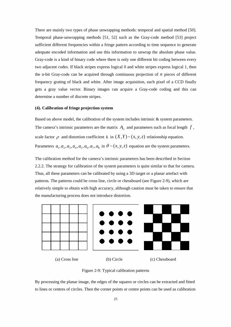
patterns. The patterns could be cross line, circle or chessboard (see Figure 2-9), which are
relatively simple to obtain with high accuracy, although caution must be taken to ensure that
the manufacturing process does not introduce distortion.
(a) Cross line (b) Circle (c) Chessboard
Figure 2-9: Typical calibration patterns
By processing the planar image, the edges of the squares or circles can be extracted and fitted
to lines or centres of circles. Then the corner points or centre points can be used as calibration
26
points. Therefore a minimum of eight sample points ( , , , )i i ix y z θ (which represents the 3D
coordinate ( , , )i i ix y z of ith sample point and its phase value θ ) need to be captured and
then substitute them to Equation (2-20), all the eight unknown parameters can be determined.
It should be noted that when the camera settings or relative position of the camera(s) and
projector changes, the calibration has to be repeated for correct measurement results.
2.2.4. Comparison of the three sensors
To measure a complex workpiece containing various detailed features, the most suitable
sensor should be selected for each particular feature. Table 2-1 presents the main
characteristics comparison of the three sensors.
The three sensors mainly cover the measurement tasks in micro domains with 2D and 3D data
acquisition. The measurement system integrating the three sensors can be exploited to
implement the general applications in dimensional measurement, RE, etc.
Table 2-1: Comparison of the main characteristics of the three sensors
Tactile probing Laser scanning Fringe projection Principle Mechanical interaction Laser triangulation Triangulation & Phase-shifting Resolution (µm) 0.01~1 0.1~100 0.1~100 Measuring range (mm) 0.01×0.01×0.01~1000×1000×1000 5×5×5~250×250×250 5×5×5~1000×1000×300 Speed Several points/second Tens of thousands of points/second Millions of points/second Init. Data type 3D (X, Y, Z) 2D (R, C) 2D (R, C)
Advantages
1. High resolution/accuracy 2. Not sensitive to the surface reflection 3. Robust and not sensitive to the ambient light
1. High scanning speed and dense point data acquisition 2. Global information acquisition 3. Suitable for the measurements of surfaces with soft/flexible materials
1. Very high scanning speed and dense point data acquisition 2. Global information acquisition 3. Suitable for the measurements of surfaces with soft/flexible materials
Disadvantages
1. Low data capturing speed 2. Limitations to its own dimension sizes 3. Sparse density of the acquired points data
1. Low resolution, noisy/redundant data 2. Limitations of occlusion and viewpoint 3. Sensitive to the surface optical conditions
1. Low resolution, large number of noisy/redundant points 2. Limitations of occlusion and viewpoint 3. Very sensitive to the surface optical conditions and ambient light
Applications
1. Primitive shapes 2. Features with known CAD models 3. Surfaces without large variations
1. Global data acquisition 2. Complex surfaces or topography measure 3. Parts with soft/flexible materials
1. Body scanning 2. Global information acquisition 3. Complex surfaces or topography measure
2.3. Multi-sensor integration in coordinate measurement
The reduction of the lead time in measurement, and the increased requirements in terms of
complexity, accuracy and flexibility have resulted in a great deal of research effort aimed at
developing and implementing combined systems based on integration of different
(homogeneous and inhomogeneous) sensors. Multi-sensor data fusion methods then are
27
employed to achieve both holistic geometrical measurement information and improved
reliability or reduced uncertainty of measurement.
A multi-sensor integration system in dimensional measurement is a measuring system which
combines several different sensors in order that the measurement result can benefit from all
available sensor information and data. While fusing data sets, characteristics such as
resolution and measuring ranges have to be considered. On the other hand, due to the different
measuring techniques and their physical working principles, different interactions between the
workpiece and sensor occur and different surfaces are captured. With a multi-sensor
integration system, particular features of a workpiece can be measured with the most suitable
sensor, and the measurement with small uncertainty can be used to correct or replace data
from other sensors which exhibit relevant systematic errors but have a wider field of view or
application range. Therefore, the merits of each sensor in the integrated system can be fully
utilized and their disadvantages can also be mitigated to improve the data acquisition
performance of the whole system.
2.3.1. Multi-sensor configuration
Sensors of a similar type which capture the same or a comparable physical object to be
measured are called homogeneous sensors. On the other hand inhomogeneous sensors acquire
different characteristics of a scene. Multi-sensor fusion performs the synergistic application of
different homogeneous and inhomogeneous sensors to execute a given measuring task. The
integration approach of multiple sensors into a multi-sensor system depends on the
application and sensor data or signal type. Durrant-Whyte [54] classifies physical sensor
configuration in a multi-sensor data fusion system into three categories as shown in Figure 2-
10: competitive, complementary and cooperative integration.
• A competitive sensor configuration is one where the sensors are configured to
measure the same feature independently in order to reduce the measurement
uncertainty and to avoid erroneous measurements. For example, an image sensor
measures the same area and the redundant information is averaged by evaluating the
mean for each pixel. Thereby all images of the series contribute equally to the final
measurement result [55].
• A complementary sensor configuration is one where the sensors do not directly
depend on each other but can be combined in order to give more complete
information about the object. Complementary sensors can be exploited to resolve the
problem of incompleteness of acquired data. An example is the data fusion of images
captured with different illumination series to achieve images with higher contrast [56].
28
• A cooperative sensor configuration uses the information provided by one or more
independent inhomogeneous sensors to drive one or more other sensors for measuring.
Often, cooperative sensor configurations allow measurands that have not previously
be evaluated to be measured. A practical example of this kind of sensors
configuration would be the case of multi-sensor integrated on the CMM platform and
use of the global information acquired by an optical sensor to guide the tactile probe
for high precision coordinate data acquisition [7].
(a) Competitive (b) Complementary (c) Cooperative
Figure 2-10: Sensors configurations in multi-sensor systems
2.3.2. Theoretical aspects of multi-sensor data fusion
The data acquired by the each sensor in the integrated system, dependently or independently,
are embedded in their own coordinate systems which are distinctly different from each other.
There are many key issues that need to be considered for data processing in order to achieve
the multi-sensor data fusion. Generally, the process of the multi-sensor data fusion based on
different information sources should include the following procedures:
• Data pre-processing
• Data registration
• Data fusion
29
2.3.2.1. Data pre-processing
The information captured by different sensors is not directly linkable, the raw data acquired
from multiple sensors are typically needed to pre-process to improve their qualities, such as
error points removal, data filtering, data reduction, etc.
(1). Error points removal
Typically parts need to be clamped before scanning. The geometry of the fixtures is scanned
by optical sensors and becomes a part of the scan data. Then the fixture data should be
eliminated manually. Some error points, for example the bed of CMM is scanned when using
optical sensor and these points obviously do not belong to the parts, they also need to be
manually removed.
(2). Data filtering
In order to better exploit the high density point data, a data filtering method is often applied.
Usage of data filtering is a common practice in RE application. Various techniques [57, 58]
are used successfully to improve point cloud quality by decreasing measurement noise.
Filtering methods will be discussed further in Section 4.2.1.
(3). Data reduction
The raw point cloud scanned by optical sensors usually contains hundreds of thousands points,
because of the high resolution of CCD cameras. Furthermore, some features on the parts are
repeatedly scanned, especially when multiple views of an object are required to capture the
full model, which also introduce a large number of redundant points. It might take a lot of
computing time if all these original points are input into triangulation process to generate a
polyhedral model of this model. Therefore the vast amounts of data need to be reduced in
order to improve the efficiency of the subsequent treatments [59].
After pre-processing, the data becomes more conducive to further processing. The pre-
processing in multi-sensor data fusion should also include the data format conversion when it
is necessary.
2.3.2.2. Data registration
Data registration has two purposes: a) 3D point data scanned from different views by the
subsystem in their local coordinate system are aligned into a global coordinate system; and b)
data acquired by different sensors are transfer into a common coordinate system. In this thesis,
data registration refers to the latter purpose.
30
As every employed sensor has its own coordinate system, which is usually different from
each other, the measured data from each other should be transformed and merged into a
common coordinate system in order to build a complete 3D model. Moreover, in the
recognition and position stages prior to the shape inspection, the digitized data from unfixed
rigid objects also needs to be registered with an idealized geometric model [60]. Therefore,
registration is one of the most critical issues and decisive steps of multi-sensor data fusion.
The transformation parameters include 3D rotations and translation. When data sets (e.g.
images) are acquired with different magnifications, transformations of proportion, sometimes
known as “scaling”, may also need to be considered. Commonly, the criterion for determining
the transformation parameters is the Least Squares Criterion. This involves the minimization
of the variance of distances of corresponding points in the sensor data or of corresponding
points in overlapping areas [11].
2.3.2.3. Data fusion
The data fusion process is performed to decide which measurement data should be integrated
into the final data set and how to handle the redundant data. The methods for data fusion
broadly belong to one of the following three techniques: estimation, inference, fuzzy or neural
methods [11]. Estimation methods, which include least square analysis [61] and weighted
average [62] are suitable to analyse the measurement systems where various results are
acquired for the same measurand or for a regression plot are combined. They are typically
applied to steady-state measurements [63]. In addition, Kalman filtering and its further
developments are usually used as model-based stochastic state-estimators in processing of
time-dependent and time-discretised digital measurement signals [64, 65]. Inference methods,
like Bayesian probability theory are used for measurement data evaluation and contemporary
uncertainty determination [66, 67].
2.3.3. Related research in multi-sensor integration
The theoretical origins of data fusion can be traced back to the late sixties, although a broad
application of these techniques did not take place until the early eighties [68]. In the
meantime, the research activities on data fusion have become very extensive and applications
to different fields have been reported, such as robotics [69], pattern recognition [70],
medicine [71], non-destructive testing [72], geo-sciences [73], military reconnaissance and
surveillance [74], etc. In the following, comprehensive research works related to
measurement and RE are presented.
31
2.3.3.1. Homogeneous optical sensors integration
The homogeneous sensors, such as cameras, laser scanners, fringe projection scanners, or
other optical sensors, are integrated into a multi-sensor system to achieve a representation of
sufficient data and/or better measurement accuracy.
One typical example is the multi-station photogrammetry network which integrates several
homogenous cameras. After calibration of the system, each observation of the object can be
captured with several images simultaneously. These images are registered to a global
coordinate to obtain a final point cloud [75]. Similarly, Aguilar, et al. [76] developed a fast
stereo metric system, which integrates two holographic optical elements, to measure free-
form surfaces of railway concrete sleepers and calculate track and rail seat dimensional
tolerances.
Moreover, a series of images captured by a single sensor (called virtual sensor in [77]) also
can be classified as a homogeneous sensor fusion problem. Instead of multiple sensors
capturing simultaneously, a single optical sensor is used to digitize the object several times in
succession to obtain a series of images with different focal depths, positions or view
orientations. Then more detailed information can be extracted from these images. Such
applications are quite widely studied and implemented due to its economy and flexibility. One
example of this integration setup is when applying the ‘shape from shading’ technique. The
setup consists of different illumination sources and a fixed camera and the camera captures a
series of grayscale images with different illuminations. The height map of the object can be
derived by the gradients analysis and calculation in these images [78, 79]. Another example is
data fusion in the fringe reflection method, also called deflectometry. From the measured
deflectometric data, different approaches allow for reconstruction with the aid of additional
knowledge or the fusion of several measurements [80].
For the three-dimensional shape measurement of complex structures for example freeform
surfaces, fringe projection systems are applied. Fringe projection can be installed in mobile
systems or in coordinate measuring machines. Two or more cameras are usually used to
capture the information simultaneously after system calibration to achieve better surface
coverage. Often, the objects to be measured are bigger than the measurement range of the
cameras or too complex to be captured in one single measurement. In a complementary
integration, multi-views are taken from different camera orientations and registered and fused
into a global coordinate system [81], problems such as shading can be solved with such a
setup [82].
32
2.3.3.2. Inhomogeneous optical sensors integration
Like the homogeneous optical sensor integration, the multiple inhomogeneous optical sensors
with different measuring principles and resolution can also be combined by cooperative or
complementary integration and applying multi-scale measuring and verification strategies.
In cooperative configuration systems, the lower resolution sensors are usually used to capture
the global information with restricted resolution. Then, a data analysis phase follows to
evaluate the information content. Further local measurements with higher resolution sensors
are required if there is not sufficient information. The resultant data is updated after
combining each additional measurement datum until the measurement tasks are fulfilled. The
system developed by Weckenmann, et al. [83] combines a fringe projection system and a
white light interferometer to measure the wear of cutting tools. A compact sensor head
combining an optical interference microscope with a scanning probe microscope in a single
measurement is demonstrated in [84]. Sokolov, et al. [85] introduces a combined confocal
sensor and scanning probe system for nano-coordinate metrology.
Some systems of complementary configurations of inhomogeneous optical sensors have also
been demonstrated by several authors. Reich, et al. proposed a multi-sensor system by
combining photogrammetry and fringe projection for shape measurement of complex objects
[86]. Schmitt, et al. [87] developed a method for the automated positioning and alignment of
fibre-reinforced plastic structures by data fusion of two optical sensors. The first sensor is an
image processing sensor for the robust detection of the local fibre orientation and the second
one is a light section sensor for the determination of the contour position of textile preforms.
The developed method was evaluated under industrial conditions through a prototype. It can
measure different quality criteria of preform structures.
2.3.3.3. Tactile and optical multi-sensor integration
Even though tactile and optical sensing technologies are widely used in data acquisition in
dimensional measurement and RE, it has been shown that each technique has its own
characteristics and applications. The requirement of both high speed and high accuracy 3D
measurement in modern measurement or RE have resulted in a great deal of research effort
aimed at developing and implementing combined systems based on integration of
inhomogeous sensors such as mechanical probes and optical sensors.
(1). Cooperative configurations
The optical sensors can be a simple video camera, a laser scanner or a fringe projection
system, which acquires the global shape information and provides the guidance information to
33
drive the CMM to execute the local exploration with a more precise tactile probe [11]. In such
systems, the advantages of the two kinds of sensors can be exploited at the same time, i.e. the
ability of the optical sensor to quickly generate the approximate shape and the ability of the
contact probe to obtain higher accurate measurement result. Nashman, et al. [88] developed a
real-time integrated system that combines a vision system and a touch probe for dimensional
inspection tasks. The low resolution vision camera is fixed on the CMM table and provides
the global information. Then the images captured by vision camera are used for the workpiece
positioning. With comparison of the image data and the data generated by the probe, the fused
information is used to guide the tactile probe to provide the final inspection data. This makes
automatic capture of specific features more efficient.
Motavalli, et al. [89] described an similar integrated sensory system combing contact probe
and two cameras for RE applications. In their work, one vertical camera is mounted on the
CMM for viewing the part from the top. The other camera is placed on a stand for viewing the
part horizontally. The processed images are then used to guide the touch probe to
automatically digitize the surfaces and create CAD representations of part prototypes.
Shen, et al. [7] presented a cooperative sensor integration system that fused a 3D active vision
(fringe projection) system and a touch probe for rapid and high precision coordinate
metrology. Intelligent feature recognition algorithms can be applied to extract the global
surface information acquired using the 3D active vision system. The obtained information can
be subsequently used to automatically guide the touch probe for rapid coordinate data
acquisition and to strategically control the probe for high precision sampling of critical
surface area.
Chan, et al. [5] developed a multi-sensor system integrating a CCD camera and a tactile probe
on a CMM platform for RE. The two sensors are fixed on the CMM arm together. The images
captured by the CCD camera are processed by neural network algorithm based method to
provide the geometric data which can be used for locating the object and planning the probing
path of the tactile sensor. The CCD images play the role of the CAD model like in CAD
model based inspection planning systems.
Similarly, Carbone, et al. [6] proposed a method to combine a stereo vision system and a
touch probe. In their method, the 3D vision system is performed to acquire a number of
clouds of points to generate a rough CAD model and to guide the mechanical probe to digitize
the surfaces. The touch point data are then imported to the CAD environment to produce the
final, accurate CAD model.
34
Chen, et al. [90] proposed a multi-sensor automatic inspection system, which combines the
coordinate measuring machine with conoprobe laser sensor and can select automatically
either of the two methods for different (simple-geometry or complex free-form) measured
objects so as to raise the accuracy and efficiency of measurement.
In summary, the implementation of above integrations tends to be cooperative where optical
sensors provide approximate shape to guide the tactile sensor for automatic digitization. This
improves efficiency, but has no direct benefit on accuracy.
(2). Complementary configurations
The complementary integration systems have also been studied by several authors.
Bradley, et al. [91], Chan, et al. [92], and Jamshidi, et al. [93], each presented separate
integrated laser-tactile systems. A laser scanner is used to scan large area surface patches and
achieve sufficient data sampling, whereas a CMM touch probe is used to precisely define the
boundary of bounding contours. Both sensors are mounted on the CMM arm. Generally, the
objects need multiple scans with different views by the laser scanner to acquire complete
point data.
Xie, et al. [94] presented a complementary sensor approach for RE. In their work, a multi-
probe measurement system integrated with a CMM, a structured-light sensor, a trigger probe
and a rotary table has been developed. The structured-light sensor is applied to scan the
profile of a part from different views, while the trigger probe is used to measure the edge and
key features of the part. Then the data generated by different modes can be merged into a
whole data set.
Sladek, et al. [8] presents a hybrid contact-optical coordinate measuring system for metrology.
The structured light system is used to acquire the surface of workpiece, then numerical
analysis is performed to calculate a set of surface points that should be finally re-measured by
the CMM. The combination of measuring systems enables the measurement of a wider range
of objects than for any single system alone and the limitations of each system are
compensated by the other.
Zhao, et al. [95] presented an automated dimensional inspection planning method using the
combination of a laser scanner and a tactile probe. The inspection features are specified and
selected based on the extracted geometry features and the associated Product &
Manufacturing Information items from a CAD model. Then a knowledge based sensor
selection method is applied to choose the suited sensor for each inspection feature.
35
In summary, complementary integration systems select different probing methods to measure
different features, often based on the principle that tight tolerance or non-surface elements
should be measured by high-precision contact probing, while elements with looser tolerance
can be scanned via optical techniques.
(3). Competitive configurations
Only limited research on competitive integration of hybrid contact-optical sensors has been
found. In the work presented by Huang, et al. [96] and Bešić, et al. [97], reduction of the
measurement uncertainties has been studied. This will be detailed in Chapter 4. This thesis
focuses on the development of a competitive integration of optical-tactile sensors for the RE
applications, which will be discussed in Chapter 4.
Moreover, ElMaraghy and Rolls [98] analysed digitizing errors between tactile probe and
laser scanning data. The integrated tactile and optical sensor calibration problem has been
researched by Shen, et al. [7, 99]. They developed an automatic camera calibration scheme,
by adopting the tip of the CMM probe to provide high-precision 3D coordinates for camera
calibration and to establish a common coordinate system for sensor integration.
2.3.3.4. Other multi-sensor integration
There are also other multi-sensor coordinate measuring setups are developed. One example is
a complementary integration system which consists of a specially designed light pen with
point shaped LED light sources which are aligned in one line with the probe stylus and a
high-resolution CCD. On the basis of knowing the positions of the light sources and the probe
stylus the 3D coordinates for the centre of the probe stylus can be calculated. During
measurement the touch trigger probe contacts the object measurement surface and the image
of the light sources is captured by dual CCD cameras. Then the coordinate rotation and
translation between the two camera coordinate systems is calibrated. Experimental results of
such a setup showed the axis orientation errors were eliminated and a better stability and
precision with an uncertainty of ±0.1 mm in the distance of 2 m [100].
To improve measurement precision, recent research activities have tried to exploit Dual
Energy Computed Tomography (CT) [101]. By scanning a specimen using different energies
and applying the knowledge about beam attenuation in the material, it is possible to combine
information of both reconstructions in order to quantify the different materials of a component.
Such integration belongs to a competitive sensor configuration application.
Furthermore, combining X-ray computed tomography with the design and components of
industrial CMMs makes it possible to achieve an accuracy enabling CT being used in
36
industrial coordinate metrology. Bartscher et al. [102] developed a complementary integration
system for RE. In their work, a fringe projection system was used to measure the outer
surface of a cast cylinder, and CT was exploited to scan inner surface. Then all information
was combined to achieve holistic geometrical measurement.
2.3.3.5. Commercial multi-sensor systems
Commercial multi-sensor CMMs are developed by using a combination of several sensors to
provide higher precise or larger ranges of the measurements. Many CMM manufacturers, for
example, Nikon, Hexagon, Werth Messtechnik, Zeiss, etc. [103], can provide the
multisensory solutions. A commercial hybrid structured light measuring system with
combinations of photogrammetric sensor and tactile probing is made by GOM Ltd. [104].
FARO Technologies Inc. develops a kind of hybrid laser and hard probe system, with a laser
line and a trigger probe mounted on an articulated arm [31].
Some commercial CMMs integrate with other non-contact methods, such as computed
tomography or fibre probe [103, 105, 106]. Additionally, multi-sensor systems based on
tracker sensors [29], interferometry or photogrammetry [107] etc., are also available.
However, the techniques and methods combining the different sensors in these systems are
usually not published due to commercial purposes.
To the author’s best knowledge, most of solutions combine the optical sensors with a tactile
probe in a complementary configuration.
2.3.3.6. Data format conversion for the system integration in CAD/CAM environment
The measurement of multi-sensor system is not isolated and should be integrated with other
activities for example PLM (Product Lifecycle Management). It is also an important issue to
embed the measurement activity into the manufacturing process. The RE should also consider
the integration problem because the measured point data which is used to reconstruct the
CAD model needs to satisfy the design intent and specifications [10].
If each respective measuring system or software outputs different data formats, data format
conversion is usually needed. The most common solution for the system integration is based
on interface standards are specified with standard file formats. Many standards and neutral
files are published for these purposes, such as IGES (Initial Graphics Exchange Specification),
STEP (Standard for the Exchange of Product Model Data) and STL (Stereo Lithography or
Standard Triangulation Language) etc. are used in this thesis for data fusion in CAD
environment.
37
2.4. Summary
Multi-sensor integration has been shown to realize measurements with holistic, better
representative and reliable information.
This chapter first presents an overview of classification for existing sensor technologies in
dimensional measurement. Then three different sensing techniques commonly used in
coordinate measurement - tactile probing, laser line scanning and fringe projection that will
be implemented in this thesis, are discussed in detail considering their working principles,
system models and calibration methods. The sensors’ measurement accuracy and ranges as
well as possible uncertainty contributions are also introduced. In general, touch tactile
probing are considered to be more accurate compared with line scanning and fringe projection,
except measuring soft surface or very thin wall when the object is affected by the tactile probe.
This is not the case in this thesis.
Then the different multi-sensor configurations and general procedures for multi-data fusion
are presented. The multi-sensor integration for surface digitization has also been introduced.
Homogeneous optical sensor integration, inhomogeneous optical sensor integration,
inhomogeneous tactile and optical probe integration, and some other system integration are
surveyed. Commercial systems for multi-sensor systems in dimensional measurement are also
described.
The following chapter will introduce a universal approach to integrate the coordinate system
of a tactile probe and optical sensors.
39
3.1. Introduction
In Chapter 2, multi-sensor integration systems were shown to be able to provide more
efficient solutions and better performances than single sensor based systems. The reduction of
the lead time in RE, and the increased requirements in terms of accuracy as well as flexibility
have resulted in a great deal of research effort aimed at developing and implementing
combined systems based on cooperative integration of inhomogeneous sensors such as
mechanical probes and optical systems, which have already been introduced in Section 2.3.3.
However, a limitation of the prosed systems is that the integration of the optical system with
the CMM generally takes place but is limited at the physical level, flexibility level and
usability level. In most multi-sensor systems, a tactile sensor (such as stylus) and optical
sensor (such as laser scanner) share the same probe fixed on the CMM arm and recalibration
is needed after each change of sensor. Furthermore, some features, because of the existence of
occlusion and diffuse reflection, are very difficult to scan using optical sensors. The views of
optical sensors need to be changed several times to acquire global information. Then the
flexibility of the system is greatly restricted because the optical sensors are fixed on the CMM
arm.
When applying multi-sensor systems, different information sources (sensors) should be
integrated in one common system. Bradley, et al. [91] and Xie, et al. [94] each presented a
complementary sensor approach for reverse engineering; a touch probe and a laser sensor are
attached to CMM Z axis− arm and two sensors coordinates system can be referenced to the
same one by measuring the same high precision ball bearing. A hybrid contact-optical
coordinate measuring system was designed by Sladek, et al. [8], but the specific unification
algorithm is not given. Huang, et al. [108] proposed an iterative registration and fusion
method for multi-sensor calibration. It uses an iterative closest point (ICP) algorithm [60] to
achieve surface fusion and Kalman filter [109] to obtain accurate surface registration.
However the ICP method and its variants [110, 111] are more suitable for registration of data
sets measured by the same or homogenous sensors (for example structured light and laser)
which have similar resolution and accuracy. It also requires a sufficient number of coincident
points from different data set to obtain an acceptable registration accuracy.
A flexible and effective approach for the integration of a CMM touch probe with optical
sensors has been proposed in this thesis. A sphere-plate artefact is developed for unification
of the hybrid system and it does not need the physical integration of optical sensors onto the
CMM arm, but includes their combination at the measurement information level. This sphere-
plate uses nine spheres rather than a traditional plate with three spheres to perform the
geometric transformation. The system unification is achieved by measuring the sphere
40
calibration board and then measurement results from all of the optical sensors and the CMM
probe head are combined into one set. This operation has to be done prior to any
measurements, after the calibration of separate systems. It is carried out only once before a
series of measurements and then the viewing position and orientation of the optical sensor can
be adjusted to scan data from as many views as necessary to completely define the workpiece
surface.
3.2. Geometric transform method for hybrid system unification
The optical scanner and the CMM tactile probe work in their own separate coordinate systems.
If the integrated system is to produce useable results, these two coordinate systems have to be
unified.
The same position surface data of a workpiece scanned from an integrated system can be seen
as a kind of rigid body movement, so the geometric transformation method can be used to
deal with coordinate unification. Since three non-collinear points can express a complete
coordinate frame, data transformation of the two systems will be achieved simply with three
different reference points and a three-point alignment coordinate transformation method can
be used to deal with coordinate system unification. Therefore, the system unification problem
for optical system and CMM tactile probe is converted to a coordinate transformation
problem, the coordinates of multiple scan data from both systems can be transformed to one
coordinate system. Coordinate transformation of 3D graphics includes geometric
transformations of translation, proportion and rotation. The coordinate transform method by
three points is derived by Mortenson and presented in [112].
3.3. Calibration board design
Since the error of each measuring reference point can be seen as equal weight value, the data
fusion errors can be seen as average distributed errors [112]. It is very difficult to obtain the
same single reference point from two different sensors (tactile and optical sensors in this case)
without imposing strict & undesirable physical constraints on the system. This is compounded
by the different measurement principles and methods of the two systems as well as different
point cloud density. For this reason, most calibration systems use a geometric feature, rather
than single point. If a reference feature point is taken as the calibration reference point every
time, the possibility of occurrence of system error, human errors and accidental errors will
increase greatly. Because three points can establish a coordinate, we can consider calculating
the centroid of a standard calibration ball and then use the sphere centre coordinate as the
datum reference point coordinate to achieve data fusion and reduce fusion errors.
41
The data fusion of 3D measurement data from different systems will be achieved through the
alignment of three datum sphere centre points. In fact, the data fusion problem is, therefore,
converted to a coordinate transformation problem. The transformation is determined by
comparing the calculated coordinates of the centres of the calibration balls obtained in
measurement conducted by the optical system.
An ball-plate calibration board (see Figure 3-1 (a)) with 9 spheres attached to it was created
for data fusion of the hybrid system. Three spheres A1, B1 and C1 form an approximate
equilateral triangle and three groups of spheres form three small approximate equilateral
triangles. The spheres are made of solid polypropylene with a matt finish and have good
roundness and sphericity (see Figure 3-1 (b)). Their nominal diameter is Ф =25.4mm with a
form error no greater than Ф =30 μm.
(a) Calibration board on CMM (b) Representative roundness of calibration balls
Figure 3-1: Spheres calibration board
3.4. Hybrid system configuration and calibration
3.4.1. Elements of the hybrid system
The integrated system (see Figure 3-2) was designed and manufactured with the following
components as shown in Table 3-1:
42
Table 3-1: The components of the integrated system
A High accuracy CMM Zeiss PRISMO system - Maximum permissible error of length measurement MPEE = (1.9+L/300) µm (ISO 10360-2:2009)
B Two CCD cameras IDS UI-1485LE-M-GL, the CCD resolution is 2560(H)×1920(V), the dimension of a pixel is 2.2 μm×2.2 μm
C Lens Fujinon HF12,5SA-1/1,4 5 Megapixel C-Mount Lens, the focal length is 12.5 mm
D Projector Panasonic PT-LB60NTEA projector with 1,024×768 pixels E Planer calibration board (12W×9H×15 mm squares) for structured light scanner
calibration and sphere-plate standard for unification of hybrid system F FaroArm Quatum laser scanner G PC Workstation
(a) Zeiss CMM and structured light system
(b) FaroArm scanner
Figure 3-2: Elements of the integrated system
3.4.2. Hybrid system calibration
The CMM and optical scanners need to be calibrated separately before measurement. A
master stylus was used for qualifying the CMM reference sphere and then the stylus system to
be used during measurement must be qualified.
43
FlexScan3D PRO 3D scanning software [113] was used in the structured light scanner system
to calibrate cameras and measure surface points. After calibration, the accuracy of the
structured light system is up to 45 µm.
The calibration for the FaroArm portable coordinate measuring machine is divided into two
stages: hard probe calibration and the laser line probe calibration. The manufacturer
specification for the non-contact (laser) volumetric accuracy is 54 µm.
3.5. Proposed method and algorithm description
3.5.1. Proposed method
The optical sensor is often the main error source for an integrated tactile-optical coordinate
system. For example in general laser line scanning is considered to be less accurate in
comparison to touch trigger probing [4]. In order to further improve the measuring accuracy
of datum-points we can consider using the centroids of spherical centres triangle rather than
the original spherical centres triangle to unify two data sets of tactile and optical sensors.
Therefore, we propose a “centroid of spherical centres” method was proposed for data
unification of multi-sensor system; the specific steps are as follows:
Step 1: Measure the sphere-plate by CMM and optical scanners separately and calculate the
spherical centre coordinates of each reference ball;
Step 2: Calculate of the centroid coordinates of spherical centres triangle measured by both
systems separately;
Step 3: Use the centroids to form two new triangles and substitute their vertexes coordinates
to Equation (3-6) to obtain R and T ; and then use rotation R and translation T to unify
two systems.
3.5.2. Mathematical model of 3D Cartesian coordinate transformation
Suppose two 3D Cartesian coordinates O XYZ− and T T T TO X Y Z− , in space Cartesian
coordinates transformation process, first the origin O is translated to another origin TO ,
then two coordinates that have same origin can be transformed into the same one through
three rotations. The transformation retaliation can be described by Equation (3-1):
o
o
oT O
xx xy y kR yz zz
= +
(3-1)
44
where [ ]TOx y z is the coordinate in O XYZ− and [ ]TTx y z is the coordinate in T T T TO X Y Z− ;
[ ]To o ox y z is three translation parameters, R is rotation matrix and k is scale factor. α , β
and γ are three rotation angles with respect to X ,Y and Z axix− ,respectively.
( ) ( ) ( )x y zR R R Rα β γ= (3-2)
1 0 0( ) 0 cos sin
0 sin cosxR α α α
α α
= −
(3-3)
cos 0 sin( ) 0 1 0
sin 0 cosyR
β ββ
β β
= −
(3-4)
cos sin 0( ) sin cos 0
0 0 1zR
γ γγ γ γ
− =
(3-5)
Then there are seven parameters o o ox y z α β γ and k , so at least three pairs of coincidence
points (nine known values) are needed to solve these parameters.
3.5.3. The principle of non-linear least squares
The Gauss-Newton algorithm [114] and Levenberg-Marquardt algorithm [115] have been
widely used in solving non-linear least squares problems.
For an over-determined non-linear equation group,
1 1 2
2 1 2
1 2
( , , , )( , , , )
0 ( )
( , , , )
n
n
m n
f x x xf x x x
m n
f x x x
= >
(3-6)
which is ( ) 0f x = . It is usually converted ( )f x into quadratic functional form in the case
where the existence of solutions cannot be determined.
Take function
2
1
1 1( ) ( ) ( ) ( )2 2
mT
ii
x f x f x f xϕ=
= = ∑ (3-7)
45
Then the minima *x of function ( )xϕ is the least squares solution of over-determined non-
linear equations, which is
1( *) min ( ) min ( ) ( )2n n
T
x R x Rx x f x f xϕ ϕ
∈ ∈= = (3-8)
Therefore, solving the over-determined non-linear equations problem is converted to a non-
linear least squares problems. By the necessary conditions for the existence of extrema, if
( )f x is differentiable in the domain, then ( )g x is the gradient function of ( )xϕ , define
( ) ( ) 0g x xϕ= ∇ = , which is
1( ) ( ) ( ) ( ) 02
Tg x x Df x f xϕ= ∇ = = (3-9)
where ( )TDf x is the Jacobian matrix,
( )
1 2
1 1 1
1 2
2 2 2
1 2
m
mT
m
n n n
ff fx x x
ff fx x x
ff
x
x x
Df
fx
∂∂ ∂ ∂ ∂ ∂
∂ ∂ ∂ ∂ ∂ ∂= ∂∂ ∂ ∂ ∂ ∂
(3-10)
First, linearize function ( )f x , then its Taylor approximations at a point kx is:
( ) ( )( ) ( ) ( )k k k kkf x Df x x x f x l x− − = (3-11)
Substituting Equation (3-11) into Equation (3-9), we have
11 ( ) ( ) ( ) ( )k k k T k k T kx x Df x Df x Df x f x−+ = − (3-12)
Equation (3-12) is the Gauss-Newton iterative method.
According to Equation (3-1), in this context Equation (3-6) can be rewritten as
46
1 1
1 1
1 1
2 2
2 2
2 2
3 3
3 3
3 3
0
o
o
o
o
o
o
o
o
oT O
xx xyy yzz zxx x
y y kR yz zzx xxy yyz zz
− − =
(3-13)
The fitting function of spatial coordinate transformation, a seven parameters problem, is a
matrix function. We can convert it into a non-linear over-determined equation group, take
space coordinates of three reference points which contains the nine coordinate values to
compose nine over-determined non-linear equations, then exploit the non-linear least squares
method to solve these seven parameters.
The specific solving steps are as follows:
Step 1: The matrix function needed to be fitted is
1 2 3 4 5 6 79 1( , , , , , , )y F x x x x x x x
×= (3-14)
Where the 3D Cartesian coordinate transformation model 7( )F x x x RX= ∆ + , 1 2 3, ,x x x are
three parameters of the translation matrix x∆ separately; 4 5 6, ,x x x are the parameters of
matrix R ; 7x is the scale factor; X is the 3D coordinates before transformation whereas y
is the 3D coordinates after transformation.
Step 2: Set up
21 2 3 4 5 6 7 1 2 3 4 5 6 7
9 1( , , , , , , ) ( ( , , , , , , ) )G x x x x x x x F x x x x x x x y
×= −∑ (3-15)
Step 3: Solve the minima of the multivariate function:
( ) ( ) 2 ( )( ( ) ) 0Tg x G x f x Df x= ∇ = = (3-16)
The Gauss-Newton iterative method is exploited to solve (3-16). We select the initial value
for the iteration, and stop the iteration when 1-norm of the vector difference of two adjacent
seven parameters is smaller than a certain threshold (for example 10-6) in the iterative process,
then the optimal solution can be derived in terms of the least squares method.
47
3.6. Experiment results and error analysis
A sphere-plate artefact with nine spheres attached to it was created for unification of the
hybrid system and a set of Matlab program was developed for the verification of this method.
The multi-sensor systems are placed in a temperature-controlled room, typical of normal
CMM applications, with the environmental temperature controlled to 20±1°C. The CMM,
structured light scanning system and FaroArm laser scanner were calibrated separately, and
then the sphere calibration board was measured by CMM touch trigger and both optical
scanners separately (see Figure 3-3).
(a) Measured from CMM (b) Measured from structured light (c) Measured from FaroArm laser
Figure 3-3: Spheres surface and centres measured from tactile and optical systems
The coordinates of centres and the radius of the spheres measured by every method were
calculated by the least squares best fit method. Table 3-2 shows the standard deviation of the
residual distances of the measurement points and the radius of the spheres.
2
1(r )
1
n
ii
rStd Dev
n=
−=
−
∑ (3-17)
where ir is the distance between each point and the centre, r is the radius of the spheres.
Table 3-2: The standard deviation on the centre and the radius of the spheres
Unit: mm Std Dev Radius ΔR (VS CMM) CMM Structured Faro Laser CMM Structured Faro Laser Structured Faro Laser
A1 3.7×10⁻³ 1.65×10⁻² 1.34×10⁻² 12.695 12.701 12.711 0.006 0.016 A2 5.7×10⁻³ 1.67×10⁻² 1.80×10⁻² 12.688 12.704 12.691 0.016 0.003 A3 4.7×10⁻³ 1.63×10⁻² 1.34×10⁻² 12.702 12.706 12.704 0.004 0.002 B1 2.6×10⁻³ 1.55×10⁻² 1.13×10⁻² 12.698 12.728 12.707 0.030 0.009 B2 6.1×10⁻³ 1.55×10⁻² 1.30×10⁻² 12.709 12.729 12.718 0.020 0.009 B3 3.6×10⁻³ 1.60×10⁻² 1.56×10⁻² 12.698 12.727 12.711 0.029 0.013 C1 3.2×10⁻³ 1.41×10⁻² 1.29×10⁻² 12.704 12.706 12.705 0.002 0.001 C2 3.0×10⁻³ 1.53×10⁻² 1.08×10⁻² 12.695 12.696 12.703 0.001 0.008 C3 4.5×10⁻³ 1.53×10⁻² 1.28×10⁻² 12.688 12.693 12.705 0.005 0.017
Average 3.7×10⁻³ 1.56×10⁻² 1.34×10⁻² 12.697 12.710 12.706 0.013 0.009
48
Taking the data measured from the CMM as the true values, because of its relatively high
measuring accuracy, then comparing with the data obtained with both optical methods, it can
be seen that the accuracy of the FaroArm laser scanner is slightly better than structured light
system in this case.
First, three spherical centres 1A , 1B and 1C were selected as benchmark reference points to
unify CMM and optical scanning systems, then centroids OA , OB and OC were used to
integrate the multi-sensor system.
Table 3-3 shows the coordinates of spherical centres of 1A , 1B and 1C , which were measured
by CMM and both optical scanners in their own local coordinates systems. For each sphere,
3,000 points therefore a total of 9,000 points, were used to obtain the fitting results.
Table 3-3: The coordinates of sphere centres
Unit: mm
CMM Structured Light FaroArm Laser X Y Z X Y Z X Y Z
A1 30.685 101.375 20.107 -28.700 -52.042 780.778 -87.255 -158.201 487.637 B1 172.079 23.386 20.162 -167.538 -134.196 788.102 64.301 -158.385 543.295 C1 169.797 184.615 20.296 -170.332 25.826 768.330 37.642 -158.521 384.334
Then 1,000 points for each sphere (total 9,000 points) were randomly selected to best-fit nine
spheres. The calculated coordinates of the centroid of the spherical centres triangle are shown
in Table 3-4.
Table 3-4: The coordinates of the centroids
Unit: mm
CMM Structured Light FaroArm Laser X Y Z X Y Z X Y Z
AO 55.890 100.907 19.998 -53.875 -53.315 780.607 -62.262 -158.370 484.267 BO 159.085 43.736 20.150 -155.192 -113.544 785.843 48.373 -158.380 525.162 CO 158.399 162.12 20.096 -158.245 3.937 771.455 29.798 -158.642 408.286
The translation vector T and rotation matrix R were solved by using above data, then the
residuals of coordinates and root mean square of residuals were compared.
3.6.1. Coordinate unification of the CMM and structured light system
The non-linear least squares algorithm was exploited to solve seven parameters. It is worth
mentioning that different initial values were selected for iteration (such as 0, 0, 0, 0, 0, 0, 1),
the algorithm was found always to quickly converge (15-20 iterations for both methods) and
obtain accurate least squares solutions even with a poor initial estimate, which shows the
algorithm is robust and not sensitive to the initial values in this case.
49
The RMSR (root mean square of residuals) was used to validate the final unification accuracy.
2 2 2
1(r r r )
3
n
iX iY iZiRMSR
n=
+ +=∑
(3-18)
where riX is the residuals of ith datum point in the X axis− direction, the rest may be
deduced by analogy.
Table 3-5 shows the residuals of coordinates and RMSR after transformation from structured
light system coordinate to CMM coordinate.
Table 3-5: The residuals & RMSR of coordinates (CMM & structured light)
Unit: mm Datum point
Traditional Method Datum point
Centroid Method X Y Z X Y Z
Residuals
A1 0.006 0.003 -0.010 AO 0.003 0.002 -0.005 A2 -0.008 0.009 -0.002 BO -0.004 0.004 -0.001 A3 0.001 -0.001 0.000 CO 0.001 0.000 0.000
RMSR 5.675×10⁻³ 2.754 ×10⁻³
It can be seen that all the residuals of coordinate transformation by using centroid method are
less than or equal the traditional method. The parameters solved by using the traditional three
spheres method are:
-0.9993 -0.0316 0.0191 4.7879R = -0.0337 0.9920 -0.1214 , -149.1387 , 0.999973
-0.0151 -0.1220 -0.9924 813.5296
S S ST T TT k
= =
Rotation angle 1 173.023α = , 1 1.095β = , 1 178.191γ = .
The parameters are solved by using the centroid method are:
-0.9993 -0.0316 0.0194 4.7849R = -0.0338 0.9920 -0.1215 , -149.1008 , 0.999976
-0.0154 -0.1221 -0.9924 813.5904
S S SC C CT k
= =
Rotation angle 2 173.020α = , 2 1.114β = , 2 178.187γ = .
3.6.2. Coordinate unification of CMM and FaroArm laser scanner
Table 3-6 shows the residuals of coordinates and RMSR of residuals after transformation
from the FaroArm laser coordinate system to the CMM coordinate system.
50
Table 3-6: The residuals & RMSR of coordinates (CMM & FaroArm laser)
Unit: mm Datum point
Traditional Method Datum point
Centroid Method X Y Z X Y Z
Residuals
A1 0.015 -0.008 -0.007 AO 0.007 -0.004 -0.003 A2 0.000 0.000 0.000 BO 0.000 0.000 0.000 A3 0.000 0.012 -0.013 CO 0.000 0.006 -0.006
RMSR 8.462×10⁻³ 4.045×10⁻³ It can be seen that all the residuals of coordinate transformation by using the new method are
also better than or equal to the traditional method. The parameters solved by using the
traditional three spheres method are:
0.9885 -0.1514 0.0023 -102.2929R = -0.0026 -0.0017 1.0000 , -178.0915 , 1.000047
-0.1514 -0.9885 -0.0021 592.6479
L L LT T TT k
= =
Rotation angle 3 90.120α = , 3 0.134β = , 3 8.708γ = .
The parameters solved by using the centroid method are:
0.9885 0.1512 0.0023 102.30660.0025 0.0018 1.0000 178.08890.1512 0.9885 0.0021 592.6
R = , ,3
1.0000 57
30
L L LC C CT k
= =
− −
− − −− − −
Rotation angle 4 90.123α = , 4 0.129β = , 4 8.697γ = .
The position and orientation of sphere plate are changed multiple times to ensure the process
is robust when their physical setup is altered. The results of the repeated tests show no loss of
accuracy.
Both experiments show that the residuals and the RMSR (see Table 3-5 and 3-6) greatly
reduce after using the centroid method to the integrate tactile-optical coordinate system, and
then the centroids can be used as datum-points for unification of the hybrid CMM and optical
systems by optimisation. If the coordinates of all nine centres are used as input for the
optimization, the unification RMSR of CMM with structured light and CMM with FaroArm
laser is 2.2565×10⁻² mm and 1.8684×10⁻² mm, respectively. The RMSR for nine spheres
give the poorest results in comparison with centroid or traditional three-sphere methods. This
indicates that excessive imprecise datum-points (data measured from optical methods) are not
conducive to improving the unification accuracy because of the induced inaccuracy in the
optimisation, it also shows the effectiveness of the new centroid approach.
51
3.7. Summary
As a response to the requirements of more effective and accurate measurement, significant
efforts are being devoted to the development of multi-sensor integration system in coordinate
measurement. The coordinates of all subsystems have to be unified if the integrated system is
to produce correct results.
The traditional three-point geometry transformation is a usual choice for coordinate
transformation. While using three datum-points for coordinate transformation and unification
of tactile-optical coordinate system, the question arises how to select optimal match datum-
points from two different sensors. Then a new development in coordinate unification called
the “centroid of spherical centres” method was introduced in this chapter, which can be used
instead of the traditional method which uses three datum-points to perform the geometric
transformation and unification of tactile and optical sensors. A sphere-plate artefact with nine
spheres is developed for unification of the hybrid system and the sphere centre points, instead
of just surface points, are exploited as datum-points. In this way some error contributions
specific to each measuring method are averaged out, which renders the fusion of the systems
more robust for practical cases.
For an integrated tactile-optical system the accuracy depends on both separate systems.
However, the main error source comes from the optical sensors and the accuracy should be
biased towards the contact method. In order to further improve the measuring accuracy of
datum-points, the centroids of spherical centres triangle rather than original spherical centres
triangle is used to unify the multi-sensor system. The same numbers of points are used to
calculate and compare the residuals of coordinates for both methods. Then a set of own
developed Matlab program was utilized for the verification of proposed method. The results
shown that the “centroid of spherical centres” method is more accurate compared to the
spherical centres method. The unification of CMM with a structured light system and a
FaroArm laser scanner shows this novel approach is simple, convenient, efficient and robust.
Both experimental results prove this novel method is more accurate than the traditional three
spheres method. Different measuring devices do not need to be placed in the same workplace.
The benefits of the proposed method are improved accuracy in coordinate unification, and
robust response to initial estimate.
In the next chapter, this method will be used to unify the Zeiss PRISMO CMM coordinate
system and Nikon LC15Dx laser scanning system.
53
4.1. Introduction
Reverse engineering is the process of creating a design model and a manufacturing database
for an existing part or prototype. The applications of RE are redesigning existing
workpieces/tools or prototype parts where the CAD model of parts are not available.
Ideally, a fully automatic RE system would exist that can make decisions, classifications and
reconstructions etc. without any user interaction. However, to the author’s knowledge, until
now there are no efficient systems have been designed which would consistently fulfill this
goal for workiece with complex geometry and freeform. There are several reasons. First, the
parts to be scanned are imperfect, owing to manufacturing errors, any damage and abrasion in
their usage. Furthermore, the point cloud data is inaccurate and noisy which is caused by
measuring system, and sometimes is incomplete because of occlusion or shiny surface.
Finally, the algorithms for processing of complex shapes are still not mature. For example,
some small geometric features cannot be successfully extracted in the segmentation process,
or cylinders are identified as parts of a revolution surface rather than cylinders. Therefore, it is
important to have a priori global characterization of the shape to be reverse engineered, and to
have a prior understanding of the measurement process at the present state-of-the-art.
When digitising an object, all surface geometry is captured including imperfections caused by
the manufacturing process and any damage the part may have suffered as well as noise
introduced by the measurement process. Typically, the part will be manually remodelled to
capture the design intent and to disregard imperfections. There are some reasons for this.
Firstly, modelling every single defect could be time consuming and therefore expensive.
Secondly, one of the main goals of RE is to reconstruct a CAD model of the workpiece.
Therefore the aim is to create a ‘more perfect’ part model representing true design intent
rather than simply copying the product being investigated. This may require a detailed
understanding of the function, depending on the part being modelled, because only then can
the design intent be correctly interpreted.
4.2. Discrete Geometry Processing in Reverse Engineering
RE technology starts with a solid artefact and constructs a geometric model by mean of
coordinate data derived from a measurement system in order to obtain a diversified and
highly creative design. The core developing procedures of RE products include:
1) Derive the coordinate data related to the existing object model using a measurement
system and construct the CAD model.
2) The constructed CAD model must be subjected to profile inspection, testing and correction.
54
3) The solid model of the RE workpiece can be rebuilt through moulding, sculpting, CNC
(computer numerical control) machining or rapid prototyping (RP).
Motavalli [116] pointed out that RE is accomplished in three steps, including part digitisation,
feature extraction, and CAD modelling. Part digitisation is the measurement process of the
object model, and the measurement result is stored in a cloud of 2D or 3D coordinate points.
Data processing based on RE involves the following operations:
• Data pre-processing
• Data registration
• Meshing
• Shape recognition and segmentation
• Model Reconstruction
Moreover, data format conversion is often required.
The classical workflow of RE of workpiece is shown in Figure 4-1.
Figure 4-1: Flowchart for a RE workpiece
55
4.2.1. Point data pre-processing
At the first step the measured data typically is pre-processed at the necessary level of
abstraction. Data pre-processing usually includes data filtering, data reduction, data ordering
etc. as described in Section 2.3.2.
The part digitisation process of RE usually involves massive point cloud data. This is
especially when the surfaces are digitized by optical methods, which often generate large
amounts of redundant points and noisy points. If all data is used in surface construction, it
usually takes a considerable time. Worse, the results may not replicate the original object
model owing to the adverse effect of measurement noise. Hence, the foremost tasks in the
processing of measurement data consist in the elimination of noise data and the reduction of
measurement data.
The purpose of the data filtering is to eliminate noise points, while keep the physical surface
features information unchanged. These motivations bring out a set of robust filtration
techniques, most of them are presented in ISO 16610 [117]. Commonly used data filtering
methods are Gaussian filtering [118], Averaging filtering [119] and Median filtering method
[120], the filtering effects as shown in Figure 4-2 [121]. Gaussian method can better maintain
the morphology of original data when performing filtering. Averaging filtration computes the
statistical average of each point for the filtration of point cloud. Median method uses
statistical mean values to filter point data, which makes this method be more suitable for the
point cloud with relatively low accuracy. In general, the Gaussian filtration is used in this
thesis for data filtration.
Figure 4-2: Three commonly used data filtering methods
56
Since not all data points measured by optical sensors are useful for the reconstruction of the
final model, it is necessary to reduce the vast amount of point data while retaining the
required feature. There have been a number of methods studied by several authors. Martin et
al. [122] devised a uniform data reduction technique using the median filtering approach.
Hamann [123] developed a data reduction method based on curvature. Points in nearly planar
surface regions are preferentially removed. Lee et al. [59] proposed a non-uniform grids
method to reduce the amount of scanned data. In thesis, curvature (Hamann) and uniform
(Martin et al.) based methods are used for data reduction.
4.2.2. Multi-view data registration
Registration is one of the most important steps of data processing in RE. The point data
acquired by multiple views are usually represented in their own coordinate systems. During
the registration process, the measurement data captured in the respective coordinate system
are aligned and transformed to one global coordinate system.
Methods that are commonly used to register multi-view data can be classified into four
categories:
1) Applying a numerical algorithm. The transformation parameters of multi-view data
include three rotations and three translations. They can be determined by minimizing the
distance between corresponding points in different surfaces. The most representative one
is the ICP (Iterative Closest Point) algorithm [60] and its variants [124-126]. Many of the
difficulties inherent in feature based methods are overcome by these methods. However,
according to the author’s best knowledge, how to find the corresponding points has not yet
been well solved. The ICP method also requires a sufficient number of conjugate points
from different data set to obtain better registration accuracy.
2) Using fiducial markers [127, 128]. The markers can be planar or 3D and are usually
adhered on or near the surface to be scanned. While the measuring sensor is taking point
data from a specific view, the 3D coordinates of the markers within the view are obtained
at the same time. The relative position and orientation of two data sets can be determined
if three or more markers are visible in both views. This method is usually fast and reliable.
However, apart from the manual preparation work before the measurement, the drawback
of this strategy is that the areas covered by the markers cannot be digitized reliably. This
problem is especially limiting when objects are small size or have abundant details.
Moreover, adhering markers on the surface is even prohibited in some applications.
3) Employing other optical or magnetic devices. For example, a FARO Laser Tracker can be
used to combine a camera and a laser tracker to track the targets fixed on the scanning
57
sensor and thereby determines the position and orientation of the sensor [31]. The
optical/magnetic tracing devices can work with large volume objects and obtain good
registration results. However, the auxiliary tracing devices are relatively heavy,
cumbersome, and of high cost for many applications.
4) Exploiting mechanical devices like CMM arms [94], turntables [129] or multi-joint robotic
arms [130]. In these solutions, either the sensor or the object to be measured is placed on
the mechanical devices, whose movement can be strictly controlled. The movement
parameters of the devices are used to automatically compute the geometric transformation
in the measurements. This method works well for some applications, yet it is limited for
measuring large objects. In addition, the use of extra mechanical devices unavoidably
reduces the flexibility and portability of the measuring system, and the effect on
measurement of each element must be well quantified.
4.2.3. Polyhedral surface generation
The scattered point sets are usually approximated to proper polyhedral surfaces in order to
build the topology structures [131]. The polyhedral surfaces are composed of polygon meshes
where the local neighbour information of each vertex can be found. The local neighbour
information is required by most computations of normal vector or curvatures on the scattered
point sets [10]. As the scattered point sets generated by optical sensors are usually noisy,
unorganized or incomplete, there have been considerable techniques developed by many
authors [132-136] for mesh generation of unorganized point sets. Among these methods, the
method developed by Alliez, et al. [134] is one of the most popular methods for surface
reconstruction of noisy defective point samples.
4.2.4. Shape recognition and segmentation
After a model is measured, the acquired point cloud data should be divided into several
smooth regions for further processing, which is called the segmentation process. The
segmentation process is used to group the initial model into a set of sub-components based on
predefined criteria. Each of the segmented regions then has an appropriate, recognizable
meaning [137].
According to different applications, the existing segmentation methods can be classified into
two categories. The first category is aimed at grouping the more natural object model into
pieces of meaningful regions based on the viewpoint of human cognition. Most of the
segmentation methods in computer graphics, biological, medical and digital heritage
applications are classified as this category. The second one is committed to segmenting
partitioning the discrete model into patches and each patch can be fitted by a single,
58
mathematically analysable shape. The applications in mechanical engineering, especially in
RE, belong to this category. For example, a mechanical part data set is segmented into data
patches of planes, cylinders, spheres, etc., belongs to this category [10].
A segmentation that extracts the edges and partitions the 3D point data plays an important
role in fitting surface patches and applying the measured data to the manufacturing process. In
RE, the segmentation has the greatest effects on product development time and the quality of
the final surface model [138]. Considerable research activities in shapes segmentation have
been explored in recent years. The methods for segmenting 3D data in engineering
applications can be generally classified into three types: edge-based, region-growing and
hybrid-based [138].
The edge-based approaches [139-142] detect discontinuities in the surfaces that form the
closed boundaries of components in the point data. Normal vectors and curvatures are
commonly used to find the boundary points. Edge-based methods are developed and applied
widely because they are simple and efficient. However, as the scanned data from
measurement sensors (especially optical sensors) are generally noisy and unreliable in edge
vicinities, finding edges is always unreliable as the computations of normal and higher-order
derivatives are sensitive to the noise [9].
Region-growing methods [143-145], on the other hand, attempt to generate connected regions
first, then proceed with segmentation by detecting continuous surfaces that have homogeneity
or similar geometrical properties. In principle, region-based methods work on the global size
of point data sets and so they are more robust to the noise than edge-based methods. However
it generates less accurate surface models than those of the edge-based method and it is also
difficult to modify the final model.
The hybrid approaches [138, 146, 147], combining the edge-based and region-based
information, have then been developed to overcome the limitations involved in edge-based
and region-based methods.
As the algorithms for segmentation are beyond this research work, the existing methods for
data segmentation are implemented for the applications to RE in this thesis. The method used
for data segmentation is introduced in Section 4.3.2.
4.2.5. Model Reconstruction
After the segmentation process, the original point set is divided into subsets which consist of
a series of polygon mesh patches or labelled points belonging to a particular region. These
subsets are needed to classify to what type of surface each subset of points belongs (e.g.
59
planar, sphere) and find that surface of the given type which is the best fit to those points in
the given subset. The surfaces subsets can be broadly classified into two categories: geometric
elements like planes, spheres, cylinders, cones; and freeform surfaces which can be modelled
using parametric surfaces such as Bezier surfaces, Basis Splines (B-Splines) or Non Uniform
Rational B-spline (NURBS) [9]. The CAD model of an object can be constructed by
combining geometric primitives or parametric patches and their boundaries [148].
4.2.5.1. Surface representations
Varieties of surfaces are studied and used in geometric modelling. In general, the surfaces are
classified as algebraic and parametric surfaces [149].
(1). Algebraic surfaces
Algebraic surfaces can be represented by an implicit equation in the form ( , , ) 0f x y z = in
3D space [150]. The advantage of algebraic representation is that manipulating polynomials
rather than arbitrary analytic functions is computationally more efficient. Another primary
advantage of algebraic surfaces is their closure properties under modelling operations such as
intersection, convolution, offset blending, etc. [149].
Quadratic surfaces are a subset of algebraic surfaces, which can be described by a general
second-order equation in x , y and z . They can be represented by 10 coefficients (Equation
(4-1)) or by a 4 4× symmetric coefficient matrix (Equation (4-2)) [151].
2 2 2( , , ) 2 2 2 2 2 2 0f x y z Ax By Cz Exy Fxz Hyz Gx Jy Kz D= + + + + + + + + + = (4-1)
[ ]1 0
1
AEFG xEBH J y
x y zF H CK zGJ K D
=
(4-2)
There are two approaches for algebraic surface fitting, one by interpolation and the other by
approximation. Interpolation is used when the function values at the measured points are
known to a high precision. Different interpolation schemes are presented by Frank [152]. In
approximation methods, the least square method (linear and nonlinear) is used to find the
coefficient of the polynomial equation [153].
(2). Parametric surfaces
60
Parametric surfaces are those which are represented in terms of two parameters u and w .
Such a representation consists of three functions ( ) , x x u w= , ( ) , y y u w= and
( ), z z u w= . Examples of these surfaces include Bezier’ surfaces, B-spline surfaces,
NURBS [149].
Bezier surfaces can be represented in a generic form as given by [154]:
, , ,0 0
( , ) ( ) ( )m n
i j i m j ni j
p u w p B u B w= =
=∑∑ (4-3)
where ,i jp are the vertices of the characteristics polyhedron that form an ( 1) ( 1)m n+ × +
array, ,i mB and ,j nB are the Bernstein polynomials. These are parametric surfaces with
Bernstein polynomials as their basis functions. The surfaces possess a convex hull property
and remain within the convex hull of the control points.
B-spline surfaces are also parametric surfaces with polynomials (instead of Bernstein
polynomials) as their basis functions defined over a knot vector [155]. The knots are
equidistant in the case of uniform B-splines while the distance is variable in the case of non-
uniform splines.
NURBS use rational polynomials as their basis functions. A NURBS curve can be
represented as [156]:
,0
,0
( )( )
( )
n
i i i pi
n
i i pi
w PN uC u
w N u
=
=
=∑
∑ (4-4)
where ip are the control points, iw are the weights and ,i pN are the normalized B-spline
basis functions of degree p defined over a knot vector (a sequence of non-decreasing
numbers):
{ }1 2 1, , , n pU u u u + += (4-5)
A NURBS surface patch can be represented by [157]:
61
, , , ,0 0
, , ,0 0
( ) ( )( , )
( ) ( )
n m
i j i j i p j qi j
n m
i j i p j qi j
w P N u N vp u v
w N u N v
= =
= =
=∑∑
∑∑ (4-6)
where ,i jP forms the control net, ,i jw represent the weights, ,i pN and ,j qN are the
normalized B-splines of degree p and q in the u and v directions defined over the knot
vectors:
{ }1 2 1, , , n pU u u u + += (4-7)
{ }1 2 1, , , m qV v v v + += (4-8)
NURBS surfaces are defined in the parameter region 0 1u≤ ≤ and 0 1v≤ ≤ only and are
undefined outside this region [158].
The algorithms for fitting parametric surfaces are divided into gridded and scattered data
fitting methods. The least squares approach is the most commonly used technique for fitting
these surfaces [149].
4.2.5.2. Boundary representation (B-rep) model creation
After direct segmentation, a set of disjoint regions is been produced, which include not only a
series of analytic surfaces, but smooth internal curves as well. The purpose of the B-rep
model creation phase is to create a consistent and contiguous model of vertices, edges and
faces, where both the adjacency relationships between the constituent elements and the
mathematical equations of underlying edge curves and surfaces are explicitly computed and
stored [148]. To present a detailed uniform approach for the final B-rep model creation would
be very difficult, so this description cannot contain all details, but the basic concepts and most
import steps will be introduced.
(1). Constraint management
For finite surfaces which are defined over a bounding box with edges (surfaces that are finite),
constraints need to be applied at the boundaries of the surfaces. While generating a solid
model from measurements of an existing workpiece, the desired continuities can be obtained
by introducing a new patch that would join the two existing surfaces with required continuity.
The constrained reconstruction on Bezier’ and NURBS patches with desired continuities is
presented by Puntambekar, et al. [159]. Multiple patches were joined at the boundaries by
62
using 0C , 1G and 1C continuity. Both parametric and analytic surfaces are successfully
joined at the boundaries with desired continuity.
(2). Surface extension
Parametric surfaces are finite surfaces and bounded by vertices and edges. When intersections
need to be computed, extension of such surfaces may be required. When the underlying
surfaces can be extended beyond the boundaries of their segmented regions, surface-surface
intersections will provide proper edge curves, which need to be limited by two end vertices.
In the case when intersection is not possible or not a true representation, blends might be
inserted or the parameters of the surfaces adjusted to make them meet smoothly [9].
(3). Stitching
Creation of the complete topological structure can be achieved by stitching together the
surfaces, edges and vertices. This is a quite straightforward process, since in the previous
phases the consistency of the geometrical and topological entities has been established.
Taking an edge loop of a given surface, the applied procedure guarantees that each real edge
is shared by another edge of a neighbouring surface and the related end vertices are identical.
Thus, taking all edges of the loops of given surfaces, all adjacent surfaces can be stitched
together [160].
4.2.5.3. Blend reconstruction and further beautification
The blends can be reconstructed after the reconstruction of the primary surfaces. The best
approximation to the appropriate radius of blends needs to be determined. Blend information
is attached to the edges and incorporated into the B-rep model. Different methods for
estimations of blend radii are thoroughly analysed in [161]. The iterative spine method and
maximum ball approach are commonly used methods, both of them are efficient and
numerically stable for blend approximation [160].
After a consistent B-rep model has been created, there are further tasks to make the
representation better from an engineering point of view. A crucial step is the “beautification”
of the final model [162]. In the presence of incomplete and noisy measured point data, the
generated model is likely to be imperfect. The exclusion of very small edges and facets,
filling of little holes, etc. are all important requirements for real-life CAD/CAM models. In
addition, for artefacts that have many important geometric properties which represent
essential information, such as symmetry, parallelism, orthogonality, concentricity, etc., such
constraints may be imposed upon the model, but this should be done under careful
consideration [9].
63
4.2.6. Reverse Engineering of sample workpiece
Figure 4-3 shows a typical workflow for RE of a sample part. The part is digitized by
the structure light system that is introduced in Section 3.5. More detailed data
processing and model reconstruction techniques based on multi-sensor technique will
be discussed further in Chapter 5.
(a) Workpiece prototype (b) Point cloud data
(c) Polyhedral model (d) Surface segmentation and recognition
64
(e) Parametric surface (f) CAD model reconstruction
Figure 4-3: RE of a sample part
4.3. Best-fit and compensation for geometric elements based on multi-
sensor system
4.3.1. Related works in competitive multi-sensor integration
When using RE methods to reproduce a given shape, the tolerance distribution of the scanned
part must be considered [9]. Multi-sensor systems allow selecting discrete probing or
scanning methods to measure part elements. The decision is often based on the principle that
tight tolerance elements should be measured by high precision contact methods, while other
more loose tolerance elements can be scanned via the faster optical techniques. Even though
the integration of optical sensors and tactile probes, which are introduced in Section 2.3.3, has
been explored in the past, such systems tend to be cooperative integration where optical
sensors acquire the global shape information of objects to guide the touch probes for
automatic point sensing.
Only limited research on competitive integration of hybrid contact-optical has been found.
Huang and Qian [96] develop a dynamic approach for integrating a laser scanner and a touch
probe to improve the measurement speed and quality. A part is first scanned by the laser
scanner to capture the overall shape. It is then probed by a tactile sensor where the probing
positions are determined dynamically to reduce the measurement uncertainty according to the
scanned data. They use a Kalman filter to fuse the data and to incrementally update the
surface model based on the dynamically probed points. Their approach can effectively save
measurement time and be able to deal with shiny surfaces, but according to the experimental
results displayed in the literature, this approach does not significantly improve accuracy of the
fused data.
65
More recently, Bešić, et al. [97] introduce a method for improving the output of a CMM-
mounted laser line scanner for measurement applications. The improvement is achieved by
using a median filter to reduce the laser scanner’s random error and by simultaneously
combining with the reliable but slow tactile probing. The filtered point data is used to
estimate the form deviation of the inspected elements while a few points obtained by the
tactile probe are used to compensate for errors in the point cloud position. The shape of the
part tested in the literature is relatively simple and only point cloud shift error caused by laser
sensor is discussed and compensated. The introduced method is very intuitive and
understandable. However, only a plane is considered in the literature and, because each point
cloud data must be filtered before shifting, the usability is adversely affected.
In addition, current commercial systems or software often only focus on processing point data
from individual sensors or techniques; the issue of where and how to effectively and
efficiently improve the accuracy of fused data is still a challenge. In particular, to the author’s
best knowledge, no relevant research has provided a method to efficiently handle integrated
measurement data in RE to use sparse accurate measurement information to improve the
overall measurement accuracy for RE applications.
Therefore, this thesis proposes an effective competitive approach for using a tactile probe to
compensate the data from a laser line scanner to perform accurate reverse engineering of
geometric features. With the coordinate data acquired using the optical methods, intelligent
feature recognition and segmentation algorithms can be exploited to extract the global surface
information of the object. The tactile probe is used to re-measure the geometric features with
a small number of sampling points and the obtained information can be subsequently used to
compensate the point data patches which are measured by optical scanning system. Then the
compensated point data can be exploited for accurate reverse engineering of a CAD model.
Since the non-surface features that cannot be scanned by optical methods can be digitised by
the tactile probe, this multi-sensor system is also a complementary configuration. The
limitations of each measurement system are compensated by the other.
4.3.2. Least squares best fit geometric elements
After a part is scanned, the acquired point cloud data should be divided into several smooth
regions for surface fitting purposes. This is called the segmentation process. Segmentation is
the problem of grouping the points in the original dataset into subsets, each of which logically
belong to a single primitive surface. Most commonly, segmentation has been viewed as a
local-to-global aggregation problem with several similarity constraints employed to form a
cohesive description in terms of geometric features. A segmentation that extracts the edges
66
and partitions the 3D point data plays an important role in fitting surface patches and applying
the measured data to the RE process. Considerable research activities in shape segmentation
have been explored in recent years, which have been introduced in Section 4.2.4. The data
sets are segmented into point-based data patches or polygon-based data patches by using
different methods. As the discrete point data is much easier to modify in comparison with
polyhedral surface, this work only considers the segmentation methods that are able to
generate the outputs for point-based data patches.
Woo et. al. [138] developed an octree approach for segmenting the scan data. First the 3D
non-uniform grids are generated by calculating the normal of each point. Then points are
assigned in the subdivided cells with different levels in size. The edge points are extracted by
selecting the points contained in the small-sized cells. Finally the segmented point-based data
patches are obtained after these edge points have been removed. This method is able to
effectively extract edge neighbourhood points and group data points and was therefore
selected for performing the data segmentation in this thesis.
After the segmentation process, the original point set is divided into subsets which can be
broadly classified into two categories: geometric elements and freeform surfaces. The
algorithms for least squares best fit of various geometric elements have been studied by
several authors [115, 153, 163]. The various geometries that are used to reconstruct a CAD
model for RE applications and studied in this thesis are planes, spheres, cylinders and cones.
4.3.2.1. Optimization algorithm
Consider a function
( ) 2
1( )
n
ii
E u d u=
=∑ (4-9)
which has to be minimized with respect to the parameters 1( , , )Tnu u u= . Here id
represents the distance of the data point to the geometric element parameterized by u . In
most cases sufficient measuring points will be taken, therefore we have m n .
(1). Linear least squares
For linear geometries (for example lines and planes), each id is a linear function of the
parameters, so that the equation in terms of exist constants ija and ib can be written as
1 1i i in n id a u a u b= + + − (4-10)
67
Our objective is to make E take its minimum value. This target can be expressed as a system
of equations of m linear equations in the n unknowns u . These equations can be rewritten
as matrix form
Au b= (4-11)
where A is the matrix whose ( ), i j th element is ija and b is the column vector whose ith
element is ib . In general m n , so we are unable to satisfy all the equations simultaneously.
Both sides of Equation (4-11) left multiply by TA , we can obtain
T TA Au A b= (4-12)
Equation (4-12) is called as normal equation. It provides the solution for u as
1( )T Tu A A A b−= (4-13)
In most cases least squares solution of u can be solved by Equation (4-13).
(2). Gauss-Newton algorithm
For nonlinear geometries (such as spheres, cylinders and cones), the functions id are
nonlinear functions of parameters. For the nonlinear problem, equations for u similar to
Equation (4-13) can be mathematically derived. However, to solve such a system we still
require an iterative type of algorithm to solve nonlinear least squares model. The reason is
the linear method given in Equation (4-13) only provides a coarse approximation. According
to our experimental results, for accurate data (such as data measured by touch trigger probe),
this model should give a best fit sphere which is very close to the result according to the full
nonlinear model; but for less accurate data such as that measured by the laser sensor, there
will be a relatively large fitting error between two methods. Therefore, the linear method can
be used to generate good initial estimates for the full nonlinear model.
The Levenberg-Marquardt algorithm and Gauss-Newton algorithm are well-known numerical
methods and have been widely used in solving non-linear least squares problems, as discussed
in Chapter 3. In this thesis, the Gauss-Newton method is used to find the minimum of the sum
of squares ( )E u . Assuming there is one initial estimate *u for the solution u , to solve a
linear least squares system of the form
Jp d= − (4-14)
68
Where J is the m n× Jacobian matrix whose ith row is the gradient of id with respect to
the parameters u
iij
j
dJu∂
=∂
(4-15)
It is evaluated at u , and the ith component of d is ( )id u . The parameter is updated as
:u u p= + (4-16)
Steps of Newton’s algorithm are repeated until it reaches a convergent point.
(3). Initial estimates
Some good initial estimates are usually required when using the Levenberg-Marquardt or
Gauss-Newton algorithms to find the solution of (u)E . If the estimate *u is poor the
subsequent estimate may be worse, which is called divergence. If the data is very inaccurate,
then the algorithm may take many iterations to converge or even stick in a local optimum
solutions. In some extreme cases, the Jacobian matrix J will even become rank deficient
and the system (Equation 4-14) will not have a well-defined solution. Therefore, good starting
values and reasonably accurate data are very necessary for algorithm fast convergence and
obtaining the global optimal solution. The least squares best fit geometric elements algorithms
are fully detailed by Forbes [153], his algorithms are exploited as fitting methods, and the
method to find initial estimates is discussed.
4.3.2.2. Least squares best fit plane
(1). Parameterization
A space plane can be specified by a point o o o( , , )x y z on the plane and the direction cosines
( , , )a b c of the normal to the plane.
o o o( ) ( ) ( ) 0a x x b y y c z z− + − + − = (4-17)
ox , oy , oz , a , b and c are the desired parameters.
(2). Algorithm description
69
When we have n points ( , , )i i ix y z , where 3n ≥ , the best fit plane should pass through the
centroid ( , , )x y z of the data and the direction cosines also have to be found. For this,
( , , )a b c is the eigenvector associated with the smallest eigenvalue of
TB A A= (4-18)
1) Find the average of the points ( , , )i i ix y z
/
/
/
i
i
i
x x n
y y n
z z n
=
=
=
∑∑∑
(4-19)
2) From the matrix A with its first column is ix x− , second column iy y− and third
column iz z− ;
3) Solve A by singular value decomposition (SVD) and choose the singular vector ( , , )a b c
corresponding to the smallest singular value.
4.3.2.3. Least squares sphere
(1). Parameterization
A sphere is specified by its centre o o o( , , )x y z and radius, r . Any point ( , , )i i ix y z on the
sphere satisfies the equation
2 2 2 2o o o( ) ( ) ( )x x y y z z r− + − + − = (4-20)
Equation (4-20) can be simplified as
2 2 2 0x y z ax ay cz ρ+ + − − − + = (4-21)
where 2 oa x= , 2 ob y= , 2 oc z= and 2 2 2 2o o ox y z rρ = + + − .
a , b , c and ρ are the desired parameters.
(2). Initial estimates
When we have n points ( , , )i i ix y z , where 4n ≥ , the Equation (4-21) can be written as matrix
form
70
2 2 21 1 1
2 2 2
1
1
i i i
n n n n n n
ax y z x y z
bc
x y z x y zρ
− + + = − + +
(4-22)
Both sides of Equation (4-22) are left multiplied by
1
1
Ti i i
n n n
x y z
x y z
− −
and simplified. Using this,
we can obtain
1 2 2 22
2 2 22
2 2 22
2 2 2
( )
( )
( )
y ( )
i i i ii i i i i i
i i i ii i i i i i
i i i ii i i i i i
i i i i i i
x x y zx x y x z xay x y zx y y y z yb
c z x y zx z y z z z
x z n x y zρ
− + +− + +− = + +− − − − − + +
∑∑ ∑ ∑ ∑∑∑ ∑ ∑ ∑∑∑ ∑ ∑ ∑
∑ ∑ ∑ ∑
(4-23)
where 2oax = ,
2oby = ,
2ocz = and 2 2 2r a b c ρ= + + − . The obtained parameters via this
model are used as initial estimates for the full nonlinear model.
(3). Algorithm description
1) Distance equation
i id r r= − (4-24)
where 2 2 2o o o( ) ( ) ( )i i i ir x x y y z z= − + − + − .
2) Objective function
2( , , , ) ( )o o o iJ x y z r r r= −∑ (4-25)
3) Derivatives
71
( )
( )
( )
1
i i o
o i
i i o
o i
i i o
o i
i
d x xx rd y yy rd z zz rdr
∂ − −=
∂
∂ − −=
∂
∂ − −=
∂
∂= −
∂
(4-26)
4.3.2.4. Gauss-Newton strategy for cylinders and cones
Both a cylinder and cone require an axis, for example a space line, to be parameterized. Any
line can be specified by giving a point ( , , )o o ox y z on the line and direction cosine ( , , )a b c ,
which constraint is 2 2 2 1a b c+ + = . So it requires six parameters to describe a line. The
distance from any point ( , , )i i ix y z to the axis is found from
2 2 2
2 2 2
i i ii
u v wd
a b c
+ +=
+ + (4-27)
where
( ) ( )( ) ( )( ) ( )
i i o i o
i i o i o
i i o i o
u c y y b z zv a z z c x xw b x x a y y
= − − −
= − − −
= − − −
Equation (4-27) is quite complicated for an optimisation routine. If we implement a Gauss-
Newton algorithm, the derivatives of this distance with respect to the parameters have to be
found, which will give rise to rather complex expressions and take a significant amount of
computing time. However, if the axis is exactly vertical and passes though the origin, then all
of the expressions become vastly simplified. To simplify computations, a copy of data is
translated and rotated so that the point ( , , )o o ox y z is at the origin of the coordinate system
and the direction cosines are aligned with the Z axis− before each iteration.
First, the data is translated so that the point on the axis is at the origin.
i i o
i i o
i i o
x x xy y yz z z
= −
= −
= − (4-28)
72
Then, the data is rotated so that the axis is along the Z axis. The rotation matrix used to
rotate the axis about the X axis− is given by
1 2 2 2 2
2 2 2 2
1 0 0
0
0
c bUb c b c
b cb c b c
−
= + +
+ +
(4-29)
The rotation matrix for rotation about the Y axis− is
2 2
2 2 2 2 2 2
22 2
2 2 2 2 2 2
0
0 1 0
0
b c aa b c a b c
Ua b c
a b c a b c
+ − + + + +
= + + + + +
(4-30)
We can rotate the data by applying the matrix 1 2U U U= × to align the cylinder or cone along
the Z axis− (see Figure 4-4).
(a) Cylinder (b) Cone
Figure 4-4: Points data translation and rotation
The iterative Gauss-Newton algorithm for cylinder and cone follows these steps:
1) Translating the data so that the initial estimate point ( , , )o o ox y z lies at the origin;
73
2) Rotation to align the axis of cylinder or cone along the Z axis− ;
3) Computing increments of the direction cosines, point on the axis and radius (cylinder) or
apex angle (cone);
4) Inverse rotation and translation transformations to the old coordinate system;
5) Updating previous values with current increments to determine the new position and
orientation of the axis;
6) Checking for convergence. If not converged, then go back to step 1.
4.3.2.5. Least squares cylinder
(1). Parameterization
A cylinder can be specified by a point ( , , )o o ox y z on its axis; a vector ( , , )a b c pointing along the axis and its radius, r .
Following Section 4.3.2.4, for a near vertical axis, we can set 1c = . Also, by knowing ox and
oy , then oz can be determined as
o o oz ax by= − − (4-31)
(2). Initial estimates
From Equation (4-27), any point ( , , )i i ix y z on the cylinder satisfies the equation
2 2 2
2 2 2
i i iu v wr
a b c
+ +=
+ + (4-32)
The Equation (4-32) is simplified; we can fit a general quadric
2 2 2 0Ax By Cz Dxy Exz Fyz Gx Hy Iz J+ + + + + + + + + = (4-33)
where
74
2 2
2 2
2 2
2 2
2 2
2 2
2 2 2 2 2 2 2 2 2 2
(b c )B (a c )C (a c )D 2abE 2acF 2bcG 2(b c ) x 2 2
2(a c ) y 2 2
2(b ) 2 2
(b c ) x ( c ) (b ) 2 2 2
o o o
o o o
o o o
o o o o o o o o o
A
aby aczH abx bczI a z acx bcyJ a y a z bcy z acz x abx y r
= +
= +
= += −= −= −
= − + + +
= − + + +
= − + + +
= + + + + + − − − −
Then initial estimates problem for cylinder can be posed as a liner least squares or eigenvalue
problem. A minimum of nine coordinate points is needed for this.
(3). Algorithm description
1) Distance equation
i id r r= − (4-34)
where ir is defined by Equation (4-32).
2) Objective function
2( , , , , , , ) ( )o o o iJ x y z a b c r r r= −∑ (4-35)
3) Normalization
2 2 2( , , ) ( , , ) /a b c a b c a b c← + +
( , , )o o ox y z ← (point on axis closet to origin)
4) Derivatives
After translation and rotation of data set, parameters ox , oy , a and b approach 0, then ir
simplifies to 2 2i i ir x y= + .
75
1
i i
o i
i i
o i
i i i
i
i i i
i
i
d xx rd yy rd x za rd y zb rdr
∂ −=
∂∂ −
=∂∂ −
=∂∂ −
=∂∂
= −∂
(4-36)
4.2.3.6. Least squares cone
(1). Parameterization
A cone can be specified by a point ( , , )o o ox y z on its axis; a vector ( , , )a b c pointing along
the axis and the apex semi-angle φ .
For a nearly vertical cone, we set 1c = and then axis o o oz ax by= − − .
(2). Initial estimates
Two methods are used to obtain initial estimates for cone fitting: normal vector based method
and geometric method.
i) Normal vector based method
The normal vector based method is usually exploited to process dense point cloud data. The
normal vector is a local geometric property of a 3D surface and specific to a given point.
Many studies have been undertaken for reliable estimation of normal vector from discrete
point data, by smooth parametric local surface association [139, 164] or by generating
polyhedral surface [138, 140].
Let ( , , )x y zn n n n= be the surface normal vector of a point on the cone (see Figure 4-5(a)),
ϕ is the angle between n and axis vector ( , , )a b c . Then φ and ϕ is complementary, that
is / 2φ ϕ π+ = . We have:
( 1, , )in v h i n⋅ = = (4-37)
where ( , , )Ti xi yi zin n n n= , ( , , )Tv a b c= , cosh ϕ= .
If Equation (4-37) is represented in matrix form, we have
76
Nv H= (4-38)
where
1 1 1x y z
xn yn zn
n n nN
n n n
=
( )H h h=
Then axis vector v and h can be solved by minimizing 2
Nv H− , / 2 arccos hφ π= − .
ii) Geometric method
The geometric method is quite straightforward. The tough trigger probe is operated on a
CMM to scan two circles perpendicular to the cone axis (see Figure 4-5 (b)). By least squares
best fitting both 3D circles, we can have their centres 1C , 2C and radii 1r , 2r . l is the
distance between 1C and 2C . Then axis of cone can be determined by 1C and 2C , φ can be
solved by
2 1arctan r rl
φ −= (4-39)
(3). Algorithm description
1) Specify t as the distance equation from the point ( , , )o o ox y z to the cone surface, then the
distance from a point ( , , )i i ix y z to the cone is found from
cos sini i id e f tφ φ= + − (4-40)
where ie is the distance from ( , , )i i ix y z to the line defined by ( , , )o o ox y z and ( , , )a b c ; and
if is the distance from ( , , )i i ix y z to the plane specified by ( , , )o o ox y z and ( , , )a b c (see
Figure 4-5 (b)).
77
(a) Normal vector (b) Parameterization of a cone
Figure 4-5: Cone fitting
After translation and rotation of the data set, parameters ox , oy , a and b approach 0, then ie ,
if and ir can be simplified to
2 2
i i
i i i
i i
e r
r x yf z
=
= +
=
(4-41)
2) Objective function
2( , , , , , , , ) ( cos sin )o o o i iJ x y z a b c t e f tφ φ φ= + −∑ (4-42)
3) Normalization
2 2 2( , , ) ( , , ) /a b c a b c a b c← + +
( , , )o o ox y z ← (point on axis closet to origin)
(0 / 2)φ π< < , if / 2φ π> then φ π φ← −
if 0t < then ( ; ( , , ) ( , , ))t t a b c a b c←− ← −
78
4) Derivatives
cos
cos
2
1
cos( ) sin( )
i i
o i
i i
o i
i i i
i
i i i
i
i i
i
i i i
d xx rd yy rd x wa rd y wb rd w
dt
w z r
φ
φ
φ
φ φ
∂ −=
∂∂ −
=∂∂ −
=∂∂ −
=∂∂
=∂∂
= −∂= −
(4-43)
4.3.3. Description of the proposed method
After multi-sensor coordinate system calibration and coordinate system unification, the
optical scanner and tactile probe measure in nominally the same absolute coordinate system.
However, two data sets measured by different sensors are unlikely to coincide absolutely,
which means there will be a measurement difference between the tactile and optical sensor.
The final aim of RE is to obtain a comprehensive, accurate CAD reconstruction model. To
achieve this goal, a data compensation method is proposed to enhance the measurement
accuracy of the point cloud data from the optical scanner. The proposed method is targeted at
manufacturing problems where a reverse engineered model with accuracy better than 50
micrometres is needed. Naturally, the scanned data points must be representative of the
geometric elements concerned.
4.3.3.1. Proposed method
After data segmentation, the data points are grouped into two types of data sets: geometric
elements and freeform surfaces. The elements which include planes, spheres, cylinders and
cones can represent 85% of machine objects [165]. Due to their simple mathematical
description and ability to model a large percentage of manufacture objects, they are widely
used in various modelling systems [166, 167]. In RE, the accuracy of final CAD model
depends on the measured point data. As the discrete point data is much easier to modify in
comparison with polyhedral surface [138], a small amount of discrete point data measured by
the high accuracy, but relatively slow tactile probe, can be used to compensate the densely
79
scanned data patches that have been measured by the fast, but relatively low accuracy optical
method. The specific method follows these logical steps:
1) Use the laser scanner to digitise the entire surface of part; and then exploit a segmentation
algorithm, as described in Section 4.3.2, to group the point data patches each belonging to a
different surface patches; these data patches will be compensated in Step 3;
2) Use the tactile probe to re-measure tight toleranced geometric features with a small number
of points to minimise the temporal cost. Then use the least squares method to best fit these
geometric elements to derive the parameters based on mathematical and numerical principles;
3) Substitute the x and y coordinates of each point measured by the laser scanner into the
parametric equations (Section 4.3.2), then the new z coordinate can be updated. Use the x , y
and new z coordinates as new point data coordinates to build point data sets. Then the
compensated data sets are exploited to reconstruct a CAD model.
Description schematic of the proposed method is shown in Figure 4-6.
Figure 4-6: Schematic of the proposed method
80
Then the new flowchart of an RE of workpiece by using multiple-sensor contact-optical
measuring system can be expressed as in Figure 4-7.
Figure 4-7: New flowchart of RE by using hybrid contact-optical measuring system
4.3.3.2. Algorithms description
The detailed algorithms for compensation of different geometric features based on multi-
sensor technique are presented as follows:
(1). Plane compensation
According to Equation (4-17), the parameters to be solved are a , b , c and ox , oy , oz . Here
we define o o o( )d ax by cz= − + + .
According to our proposed method, the new z coordinate can be derived by:
81
( ) /Ni i iz ax by d c= − − − (4-44)
To compare the normal of the plane, we let 1d = .
The workflow for plane compensation can be described in Figure 4-8.
Figure 4-8: Flowchart of plane compensation by using multi-sensor measuring system
(2). Sphere compensation
According to Equation (4-20), the parameters to be solved are ox , oy , oz and r . First we translate a copy of the data so that the centre of the sphere is at the origin.
( , , ) ( , , ) ( , , )i i i i i i o o ox y x x y x x z y= − (4-45)
Then the value of the new z coordinate can be derived by
2 2 2Ni i iz r x y= ± − − (4-46)
Here two values of Nz are obtained that will fit the sphere. To determine which one is needed,
the value of ( )z i is determined to be positive or negative:
0( ) ( ) ;
( ) ( ;
)
)
(
N N
N N
z i z ielsez i z ie d
if i
n
z >
=
= −
In some cases the solving results of Nz includes imaginary parts, which means that the original points are beyond the scope of the sphere to be fitted. We have to delete those points in the new point data coordinates. In fact, this is an effective way to exclude noisy data.
Finally, the origin is translated by an amount equal and opposite to the vector in Equation (4-45), above.
82
The workflow for sphere compensation can be described in Figure 4-9.
Figure 4-9: Flowchart of sphere compensation by using multi-sensor measuring system
(3). Cylinder compensation
For cylinder and cone compensation, the proposed method is inverse shifting of the data so that the point ( , , )o o ox y z on the axis lies at the origin. Inverse rotation of the data set is then
performed using the transpose of rotation matrix U which rotates ( , , )a b c to coincide with
Z axis− . Again, we will translate and transform the data back after compensation. Then the value of the new Ny coordinate can be obtained by
2 2Ni iy r x= ± − (4-47)
The method for determining the positive and negative of Niy is much the same as that for spheres.
The workflow for cylinder compensation can be described in Figure 4-10.
83
Figure 4-10: Flowchart of cylinder compensation by using multi-sensor measuring system
(4). Cone compensation
After data set translation and rotation, the value of the new Niy coordinate of cone can be calculated by
2 2( )Ni i iy r kz x= ± − − (4-48)
where tan( )k φ= .
The workflow for cone compensation can be described in Figure 4-11.
4.4. Summary
In many industry areas, it is desirable to create geometric models of existing objects for which
no such model is available. RE of workpiece prototype for CAD/CAM is a rapidly discipline
where interest is currently high. After elaborating the purpose of RE and the main application
areas, the most important data processing steps are outlined and various reconstruction
strategies are presented. Specific issues addressed include data pre-processing of points and
multiple view registration, polyhedral surface generation and segmentation, related surface
representations and creating consistent and accurate B-rep models. The classical workflow of
RE is also introduced and finally reconstruction of a geometric model of the prototype is
described.
84
Figure 4-11: Flowchart of cone compensation by using multi-sensor measuring system
The algorithms for computing least-squares best fit geometric elements and initial estimation
for the Gauss-Newton algorithm are detailed in this chapter. These algorithms are exploited
for best fitting and the compensation of multiple-data measured from multi-sensor system.
With the point cloud data acquired using a laser scanner, intelligent feature recognition and
segmentation algorithms can be applied to extract the global surface information of the object.
Then the high precision touch probe is used to re-measure the geometric features with a small
number of sampling points. The obtained information can be subsequently used to
compensate the point data patches which are measured by the optical system.
Finally, a novel method for the compensation of fused data measured from integrated multi-
sensor system based on geometric algebra approach is proposed. A new workflow for RE of
workpiece by using a multi-sensor contact-optical measuring system is also presented.
Validation of the proposed method is described in Chapter 5.
86
5.1. Multi-sensor system configuration
5.1.1. System overview
The multi-sensor measurement system used for data acquisition is a Nikon LK V 15.10.8 HA
high accuracy ceramic bridge CMM which integrates two different sensors: a Renishaw
SP25M touch trigger probe and a Nikon LC15Dx single stripe laser scanner. It operates in a
temperature-controlled room, typical of normal CMM applications, with the environmental
temperature controlled at 20 ± 0.2 °C. The measurement system contains two parts: the
dimensional measurement equipment which include the CMM and the two sensors; the
measurement software packages which is used to support the measurement execution and data
acquisition. Figure 5-1 gives a general overview of the measurement system. The two sensors
integrate with the CMM via the Renishaw PH10MQ articulating motorised probe head; only
one sensor can operate at any given time. The software platform CAMIO7 multi-sensor CMM
measurement software is used for measurement planning and data acquisition.
Figure 5-1: Nikon LK V 15.10.8 HA high accuracy ceramic bridge CMM
87
Table 5-1 shows the main specification parameters of the Nikon LK V 15.10.8 HA CMM, it
can be used for touch trigger and non-contact inspection, digitizing, scanning, reverse
engineering, etc.
Table 5-1: Nikon LK V 15.10.8 HA high accuracy ceramic bridge CMM
Technical figure Parameter Value
Volumetric accuracy 1.5 um+L/350 Repeatability 1.5 um Velocity up to 50 m/min Acceleration up to 5400 m/min2
5.1.2. Sensors description
(1). Renishaw SP25M touch trigger probe
The Renishaw SP25M touch trigger probe comprises two sensors in a single probe system and
is able to execute scanning and touch-trigger probing. It is also compatible with different
scanning modules, which can carry M3 styli with lengths from 20 mm to 400 mm. Table 5-2
presents the specifications of the SP25M [168].
Table 5-2: Specifications of the Renishaw SP25M scanning probe system
Technical figure Parameter Value
MPEE (ISO 10360-2) 1.6+L/375 μm Resolution < 0.1 µm
Over-travel range ±2.0 mm in X and Y 1.7 mm in +Z 1.2 mm in –Z
Probe attributes Pivoting motion in XY plane with translation in Z direction
Stylus lengths 20-400 mm Spring rate 0.2-0.6 N/mm
(2). Nikon LC15Dx laser scanner
Nikon LC15Dx laser scanner works on the laser triangulation principle as described in
Chapter 2 and is a high accuracy range laser scanner. The acquired data of LC15Dx are pixel
coordinates on 2D images which should be converted to the 3D spatial coordinates of the
measured points through calibration. The specifications of the LC15Dx laser scanner are
listed in in Table 5-3. The Nikon LC15Dx laser scanner can be used to measure 3D geometric
deviations and surface digitization with high point density, etc. When scanning, the surfaces
88
to be measured should be covered by the field of view (FOV) of the laser scanner. It is also
able to digitise shiny surfaces by changing the intensity of the laser. However this is at the
cost of sacrificing accuracy.
Table 5-3: Specifications of the Nikon LC15Dx laser scanner
Technical figure Parameter Value
MPEE (ISO 10360-2) 3.6+L/375 μm Multi-stylus test (MPEAL) 6 μm
Resolution (point spacing) 22 μm
Data acquisition (approx.) 70,000 points/sec
Points per line (approx.) 900 Measuring temperature range
18-22 °C (64.4-71.6 °F)
FOV 18×15 mm Laser type Class 2 (660 nm) Weight 370 g
(3). Comparison between two sensors
The two sensors can cover the measurement tasks in macro domains with 2D and 3D data
acquisition with tactile or non-contact sensing techniques. Each of them has its own
significantly distinct advantages and disadvantages. A complex workpiece is usually
comprised of various detailed features, the most suitable sensors must be selected for
measurement of each particular feature. The table 5-4 presents the main characteristics
comparison of the two sensors. The measuring system integrated with the two sensors can be
exploited to capture the surface data in RE and dimensional metrology.
89
Table 5-4: Comparison of the tactile probe and the laser sensor
Renishaw SP25M probe Nikon LC15Dx laser scanner Principle Kinematic touch trigger Laser triangulation Resolution < 0.1 μm 22 μm Speed 1~2 point/second 70,000 point/second Init. Data type 3D (X, Y, Z) 2D (R, C)
Advantages
1. High resolution/accuracy 2. Not sensitive to the surface
reflection 3. Robust and more adaptable
to the ambient light
1. High scanning speed and dense point data acquisition
2. Global information acquisition 3. Suitable for the measurements of
surfaces with soft/flexible materials
Disadvantages
1. Low data capturing speed 2. Limitations to its own
dimension sizes 3. Sparse density of the
acquired points data
1. Low resolution, noisy/redundant data 2. Limitations of occlusion and
viewpoint 3. Sensitive to the surface optical
conditions
Applications
1. Primitive shapes 2. Features with known CAD
models 3. Surfaces without large
variations
1. Global data acquisition 2. Complex surfaces or topography
measure 3. Surfaces with soft/flexible materials
5.2. Case study one: simple geometric shapes
Measurement errors of laser line scanning, their components and sources have been
investigated by several authors. Major contributions to the level of noise data are surface
optical properties, in-plane and out-of-plane angles and scanning depth [4, 15, 18, 169].
This section first investigates details of measurement results in usage of lase line scanning in
dimensional measurement applications. Then the feasibility and robustness of the proposed
approach are examined.
The inspection values based on measured and processed results from the Nikon LC15Dx laser
scanner are compared to reference values obtained by the SP25M tactile probing. Three
different laser scanner measurement errors (position errors, orientation errors and size errors)
were investigated by measuring one sphere and one cylinder and comparing the fitting results.
A sphere (Part A) with nominal radius of 12.7 mm and a cylinder (Part B) with nominal
radius of 14.55 mm were used to investigate the measurement errors and test the robustness
and feasibility of the introduced method. The sphere is made of solid polypropylene with a
matt finish and has good roundness and sphericity. The cylinder is made of aluminium alloy
and has a shiny surface. Both parts were scanned by the LC15Dx laser scanner and SP25M
touch probe five times, separately. During laser scanning, the distance between the surface of
the artefact and the laser scanner in various orientations was kept constant by using the
90
optimal distance to minimize influence of the scan depth to measurement error. Then the
original point data scanned by the laser sensor was compensated by using data measured by
the tactile probe. The first set of data measured by the tactile probe was used to compensate
the data scanned by laser sensor separately.
Figure 5-2 shows the coordinates of the sphere centre and radii calculated from the laser,
tactile probe and compensated data; X axis− is the scan sequence (five times for each
method).
(a) X coordinates (b) Y coordinates
(c) Z coordinates (d) Sphere radius
Figure 5-2: Fitting results of sphere using different methods
Figure 5-3 shows the normal vector of axis of cylinder and radii calculated from the laser,
tactile probe and compensated data.
(a) Normal vector a (b) Normal vector b
91
(c) Normal vector c (d) Cylinder radius
Figure 5-3: Fitting results of cylinder using different methods
Standard deviations of fitting results of Part A and Part B are displayed in Figure 5-4. It can
be seen that the deviations measured from SP25M probe are significantly less than those
measured from LC15Dx laser scanner.
(a) Sphere (Part A) (b) Cylinder (Part B)
Figure 5-4: Standard deviations of fitting results of different methods
Overall, the fitting results show high stability of the data measured from the tactile probe. By
comparing the centres measured from both sensors, which is presented in Figure 5-2, we can
see that there are position errors between two sensors; Figure 5-3 shows the orientation errors
between the two sensors by comparing the normal vector of axis of cylinder; Figure 5-2 and
5-3 present the size errors of sphere and cylinder measured from multiple sensors, the shape
sizes scanned from laser sensor are slightly bigger that those measured from tactile probe.
Through the above data analysis, it can be seen that all three errors, which are position error,
orientation error and size error, are observed in the laser line scanning by using tactile probing
as a reference. The systematic errors between laser sensor and tactile sensor and standard
deviations significant decrease after the laser data set is compensated.
92
5.3. Case study two: plane-sphere-cylinder-cone
Part C (Figure 5-3 (a)) is made of aluminium alloy 5083 and designed with only geometric
features. After data segmentation, these geometric elements are exploited to prove the concept
proposed in this thesis. The elements on the parts include the most typical of geometric
features: plane, sphere, cylinder and cone. The workpiece was located on the bed of the CMM
and fixed by clamps when performing the measurement.
The laser sensor was used for surface global information acquisition. Because of the
reflection of the surface, the intensity of the laser was changed to scan the shiny part. The
views of the laser scanner were adjusted by the Renishaw PH10MQ probe head to cover the
full surface. A trial version of the commercial software, Geomagic Wrap 2013, was used for
performing the data pre-process tasks of data denoising and reduction, etc. The data scanned
by laser and tactile probe are shown in Figure 5-5 (b) and (c), respectively. Figure 5-5 (d)
displays merged and organized point cloud data.
(a) Part C to be measured (b) Data measured from laser scanner
(c) Points measured from tactile probe (d) Merged data
Figure 5-5: Points data measured using multi-sensor system
93
The data measured by the laser scanner was segmented by Woo’s method which has been
described in Section 4.3.2 (see Figure 5-6). Then the large amounts of unordered points that
belong to different geometric element patches can be compensated by a small amount of point
data using the tactile probe.
(a) Plane (b) Sphere
(c) Cylinder (d) Cone
Figure 5-6: Point cloud data segmentation
There is a desire to determine how many points must be captured by the tactile probe to
achieve the desired representation of geometric elements. Traditionally, the number of
sampled points is required to be ten times the number of parameters in the model [170].
However, in this experiment more sampled points were taken and the fitting results were
compared.
The fitting results for different features using different methods and their standard deviations
are listed in Table 5-5. All the parameters in the table have been introduced in Section 4.3.2.
All the algorithms are introduced in Section 4.3.3 and the experimental results are calculated
by utilizing own developed Matlab program.
94
Table 5-5: Fitting results using different methods (Dimensions in mm)
Feature Parameter Laser Tactile robe (MIN points)
Tactile probe (more points) Compensated
Plane
Points 59,064 60 1,031 59,064
a -0.0001 0.0000 0.0000 0.0000
b 0.0000 0.0000 0.0000 0.0000
c 1.0000 1.0000 1.0000 1.0000
d 1 1 1 1
Std Dev 1.278×10⁻² 7.4×10⁻⁴ 6.8×10⁻⁴ 0
Sphere
Points 45,071 40 930 45,071
ox 0.0061 0.0022 0.0025 0.0027
oy 0.0090 -0.0032 -0.0031 -0.0031
oz 51.9679 51.9717 51.9719 51.9716
r 12.0080 12.0006 12.0006 12.0009
Std Dev 9.62×10⁻³ 7.1×10⁻⁴ 6.7×10⁻⁴ 2.67×10⁻³
Cylinder
Points 69,426 70 1,270 69,426
a -0.0001 0.0000 0.0000 0.0000
b 0.0001 0.0001 0.0001 0.0001
c 1.0000 1.0000 1.0000 1.0000
r 50.0175 50.0106 50.0107 50.0108
Std Dev 1.448×10⁻² 8.4×10⁻⁴ 8.1×10⁻⁴ 1.37×10⁻³
Cone
Points 69,030 70 1,503 69,030
a -0.0001 -0.0002 -0.0003 -0.0001
b 0.0001 0.0005 0.0006 0.0006
c 1.0000 1.0000 1.0000 1.0000
φ 29.9982 29.9976 29.9975 29.9979
Std Dev 1.522×10⁻² 9.2×10⁻⁴ 1.25×10⁻³ 1.89×10⁻³
All the computing tasks were operated on a desktop computer with an AMD Phenom II×4
970 3.5 GHz processor and 8GB RAM. Table 5-6 presents the computing time of data
updating for different features.
Table 5-6: Computational time
Feature Plane Sphere Cylinder Cone Number of points 59,064 45,071 69,426 69,030
Computational time (s) 0.004354 0.023247 0.063289 0.144763
95
The meshed surfaces before and after compensation are illustrated in Figure 5-7 (a) and (b),
respectively.
(a) Mesh surface before compensation
(b) Mesh surface after compensation
Figure 5-7: Mesh surface
96
From the above fitting results we can draw several conclusions:
1) It has been shown that ten times the number of parameters is a sufficient number of measurement points using the tactile probe, considering its measurement uncertainty. This result is consistent with the conclusion introduced in literature [170].
2) After compensation, the quality of the point data measured from the optical sensor has been greatly improved (see Figure 5-7). In theory, the compensated data has the same accuracy as the data measured from the tactile probe.
3) The compensated data is more robust and more likely to be identified by recognition algorithms, and is therefore more conducive to process in the next step of model reconstruction.
5.4. Case study three: complex housing
5.4.1. Multi-data acquisition
Part D is a more complex housing (Fig. 8 (a)) modified from literature [95],which has a shiny
metal surface. It also contains the typical geometric features and freeform characteristic.
Therefore, it should be an interesting case to test and verify the proposed approaches for
multi-sensor data fusion for RE. The workpiece was located on the bed of the CMM and fixed
by clamps, which are supplied by the manufacturer when performing the measurement.
(a) Laser scanning (b) Tactile probing
Figure 5-8: Tested workpiece and sensor selection
The laser sensor was used for surface global information acquisition (Figure 5-8 (a)). Because
of the reflection of the surface, the intensity of laser was changed to scan the shiny workpiece.
Two poses of the part were required in order to acquire entirely the point cloud data from the
top and the bottom of the workpiece. The datum plane and tight tolerance features need to be
measured more accurately, and the inner holes are difficult to scan by laser scanner because
of occlusion. Therefore an SH25-1 stylus holder with a M3 40 mm stylus carried by the
97
SP25M tactile probe was exploited to measure these features (see Figure 5-8 (b)). All point
cloud data was scanned manually by the operator.
Table 5-7 presents the numbers of points of raw data, scanning views and measurement time.
Table 5-7: Numbers of points and scanning time
Methods Views Number of points Measuring time (min:s)
Laser - top 21 6,573,959 12:04 Laser - bottom 12 3,840,678 7:15 Tactile probe - 4,143 14:55
The raw data for the tip & bottom surfaces scanned by the laser are shown in Figure 5-9 (a)
and (b), respectively. The points scanned by touch probe are shown in in Figure 5-9 (c). First,
the top and bottom surface point data were registered to the same coordinate system, the
method proposed in reference [171] was exploited to align the two piece of data. The raw
points cloud data acquired by the laser scanner contains a large number of noise and
redundant data. The initial acquired point data is imperfect, which increases the difficulty of
the geometry processing in the next stages. Therefore, data denoising and filtering processes
are necessary to improve the quality of initial point cloud data. As the data pre-processing
procedures are beyond the study scope of this thesis, here the existing Geomagic Wrap
software was used to do the pre-processing and improve the quality of the raw data. Figure 5-
9 (d) shows the processed and aligned point cloud data.
(a) Top surface scanned by laser (b) Bottom surface scanned by laser
98
(c) Data scanned by touch probe (d) Points data after pre-processing and register
Figure 5-9: Examples of the acquired data
5.4.2. Discrete geometry processing and CAD model reconstruction
5.4.2.1. Point data segmentation and compensation
The merged and organized point cloud data measured from both sensors (Figure 5-10 (a)) was
segmented by a feature recognition algorithm. Figure 5-10 (b) shows the point cloud data
after segmentation. Then the vast amounts of unordered points belonging to different
geometric element patches can be compensated using a small amount of point data from the
touch probe. This process is realized by utilizing own developed Matlab program.
(a) Merged points (b) Points data segmentation
Figure 5-10: Points cloud data after segmentation
5.4.2.2. Triangle mesh generation and shape recognition
The compensated point data is used to generate a polyhedral surface which is shown as Figure
5-11 (a). Figure 5-11 (b) illustrates the shape recognition on the mesh surface.
99
(a) Triangle mesh surface (b) Shape recognition
Figure 5-11: Points cloud data after segmentation
5.4.2.3. Model Reconstruction
After trimming and stitching the parametric surface (Figure 5-12 (a)) a solid CAD model is
generated. Figure 5-12 (b) shows the reconstructed CAD model in the SolidWorks 2013
environment (both uncompensated and compensated models are visually the same).
(a) Parametric surface (b) CAD model rebuild
Figure 5-12: CAD model reconstruction
5.4.3. Measurement speed and accuracy comparison
5.4.3.1. Measurement speed comparison for sensors
In the digitizing process for Part D, the actual scanning time was 19 min 19 s and the tactile
probing time was 14 min 55 s, therefore the total measuring time was 34 min 14 s (Table 5-7).
100
Finally 105,122 points scanned by laser sensor were retained after data reduction to generate a
satisfactory mesh surface for CAD model reconstruction, and 2,019 points measured from
tactile probe were exploited to compensate the laser scanned data.
In comparison, if we assume that the tactile probe senses the part at the speed of 4-5 points
per second, based on the scanning speed presented in Table 5-7, the time to digitise the part
using only a tactile method would be a minimum of six hours. The integration of the laser
scanner and CMM therefore leads to much faster measurement than the tactile method alone.
5.4.3.2. CAD model accuracy comparison
An independent high accuracy Zeiss PRISMO system, which has been introduced in Section
3.4.1, was exploited to provide an independent evaluation of the accuracy of the reconstructed
CAD model. The method described in Chapter 3 was used to unify the two coordinate
systems. Table 5-8 shows the residuals of the coordinates and RMSR after transformation
from Nikon LC15Dx laser scanning coordinate system to the Zeiss CMM coordinate system.
Table 5-8: The residuals & RMSR of coordinates (Zeiss & Nikon LC15Dx)
Unit: mm Datum point
Traditional Method Datum point
Centroid Method X Y Z X Y Z
Residuals
A1 0.001 -0.005 0.006 AO 0.001 -0.004 0.003 A2 -0.006 0.004 0.003 BO -0.004 0.001 0.003 A3 0.008 0.007 0.008 CO 0.000 0.000 0.000
RMSR 5.774×10⁻³ 2.403×10⁻³
It can be seen that all the residuals of coordinate transformation by using centroid are superior
to the traditional method, which further indicates the effectiveness of the method proposed in
Chapter 3.
To validate the final reconstructed CAD model quality, we use the root mean square (RMS)
error distance to check the accuracy of the constructed CAD model CADS . However in
practice, the actual surface may be difficult or even impossible to obtain. A large number of
accurate CMM probing points can be exploited as the reference points on the actual surface
[172]. The RMS can then be obtained by
2
1( , )
NT Si i
id p p
RMSN
=
=∑
(5-1)
101
where Tip is the sampled point using CMM tactile probe, N is the number of those sampled
points. Sip is the projected point to the constructed surface of CAD model CADS , and
( , )T Si id p p is the distance between T
ip and Sip .
From Figure 5-13 & 5-14, it can be seen that see the accuracy of reconstructed CAD model
after compensation, especially the geometric elements rebuilt from the fused data, has been
greatly improved.
Table 5-9 shows the RMS comparisons of the reconstructed CAD models. We can also see
that the result indicates that the accuracy of the geometric elements of reconstructed CAD
model has been greatly improved after compensation.
Table 5-9: RMS comparison
RMS (mm) Before compensation After compensation Geometric features only 0.045 0.007
Geometric features & freeform 0.074 0.062
5.4.4. Further improvement of the reconstructed model
The final aim of RE is to create a ‘more perfect’ model representing true design intent as
previously described, which means it does not need to simply copy the original product to be
reverse engineered. Of course, this requires a detailed understanding of the function and a
priori global characterization of the shape of the part.
For example, by analysing the design intent of the housing workpiece, the plane A and B are
supposed to be coplanar, plane A and C should be parallel; and cylinder E and F should be
coaxial (see Figure 5-12 (a)). Then these adjustments can be realised in the compensation
process. In other words, through changing the parameters which are calculated from data
measured by touch probe, the data patches measured from optical sensors can be corrected. In
this way a ‘more perfect’ CAD model can be created.
The methods provided in this thesis simplify the problem, so could eventually facilitate an
automatic system capable of detecting these relationships.
102
(a) Before compensation
(b) After compensation
Figure 5-13: The comparison of geometric features
103
(a) Before compensation
(b) After compensation
Figure 5-14: The comparison of geometric features & freeform
104
5.5. Summary
This chapter aims to validate the proposed methods in Chapter 4.
Firstly, three different measurement errors - position errors, orientation errors and size errors
of the laser line scanner are tested by using a SP25M tactile probe as a reference. Then the
feasibility and robustness of the proposed approach are examined.
Secondly, a part with common geometric features is selected to test the introduced method
after data segmentation. The workpiece is fully digitized using the multi-sensor system -
Nikon LK V 15.10.8 HA high accuracy ceramic bridge CMM. A set of programs, based on
Matlab R2011b platform, has been developed for verification of the proposed methods of data
fusion based on multiple sensors. The experiment results show that the algorithms provide
satisfying performances and the vast amounts of unordered points measured from the optical
sensor are converted to ordered and accurate data points after compensation.
Finally a workpiece that contains typical geometric features and freeform characteristics is
investigated to further verify the proposed method. The multiple data are acquired by laser
scanning and touch probing in both complementary and competitive multi-sensor
configurations. First the acquired point data of the workpiece are pre-processed in the
commercial software Geomagic Wrap; then the optical scanned data are compensated by
using own developed Matlab program; finally the compensated point data are processed in the
SolidWorks environment to build the CAD model. The measurement speed using different
methods is compared and the accuracy of the reconstructed CAD models is evaluated by an
independent high precision CMM. Further improvement of the reconstructed model has also
been discussed.
106
6.1. Summary
In many areas of industry, it is desirable to create geometric models of existing objects for
which no such models are available. Reverse engineering (RE) is a rapidly evolving discipline
intended to meet these needs. RE typically starts with measuring an existing object so that a
surface or a solid model can be deduced in order to exploit the advantages of CAD/CAM
technologies. For rebuilding the workpiece, the holistic information of the workpiece as one
entity must be known. This includes dimensional and geometrical, macro and micro
geometric surface related characteristics with tolerances, and sometimes information
regarding the interior structure of the part. At present, no single sensor solution can efficiently
provide this information. Multi-sensor data acquisition and fusion is an effective approach to
solve this problem.
Multi-sensor data fusion has been shown to be able to realize measurements with holistic,
more accurate and reliable information. Applications of multi-sensor integrated systems in 3D
measurement are of increasing importance in quality control, RE and many other industrial
fields. This thesis investigates a competitive and complementary fusion of integrated tactile-
optical coordinate measuring system for RE applications. It is shown to fulfil the increasing
requirements for rapid and accurate reconstruction of the CAD model of a workpiece with
complex shapes.
A modified calibration method for referencing both tactile and optical sensors in one unified
coordinate system is presented. As the contact probe and optical scanner work in their
separate coordinate systems, these coordinate systems have to be unified to produce correct
result. A sphere-plate artefact with nine spheres is developed for data integration of multi-
sensor system and experimental results prove this novel approach is more accurate than the
traditional three spheres method. After unification, the combined data from both systems is
treated as being from one source. In comparison to using a Iterative Closest Point (ICP)
method to register the data captured by multiple sensors, this new approach, presented in
Chapter 3 is more robust and convenient.
A new workflow for RE of workpiece based on integrated tactile-optical coordinate
measuring system is also developed. The new workflow allows a more reliable source to
compensate less accurate information.
A set of algorithms for computing least squares best-fit discrete geometry elements is
summarized. Based on the existing methods, the fitting algorithms for the four most common
geometric features are detailed and the initial estimates methods for solving nonlinear least-
squares problems are presented. In general, laser line scanning and fringe projection are
107
considered to be less accurate compared with tactile probing. Then the parameterisations of
the elements can be obtained through least-squares fitting of a small amount of points probed
by a tactile sensor, and then these parameterisations can be used to compensate the vast point
cloud data scanned by the optical method. This combination of measuring systems enables the
improvement of the measurement performance. A small amount of discrete point data
measured by the high accuracy, but relatively slow tactile probe, can be used to compensate
the densely scanned data patches that have been measured by the fast, but relatively low
accuracy optical method. Unlike most of the other hybrid contact-optical systems based on
cooperative configuration, this work focuses on developing a competitive system to ensure
the accuracy of measurement results and reduce the measuring time simultaneously.
A new competitive approach for rapid and accurate RE of geometric features from multi-
sensor systems based on a geometric algebra approach is proposed. A set of programs based
on the Matlab R2011b platform has been developed for the verification of the proposed
method. Then the compensated data is processed to rebuild a CAD model in the SolidWorks
2013 environment.
Other existing cooperative multi-sensor configuration approaches only use optical sensors to
capture the global surface information of the object and then guide the slower tactile probe to
digitize the surface. In the presented method, the multiple data sets are acquired by laser
scanning and tactile probing in both competitive and complementary multi-sensor
configurations. With the point cloud data acquired using a laser scanner, intelligent feature
recognition and segmentation algorithms can be applied to extract and segment the point
cloud data. Then the tactile probe is used to re-measure the holes, which are difficult to
measure by laser sensor, and tight tolerance geometric features with a small number of
sampling points. The obtained information can be subsequently used to compensate the point
data patches which are measured by laser sensor, as described in Chapter 4.
The results of the four case-study experiments presented in Chapter 5 show that the
algorithms provide satisfactory performance and the vast amounts of unordered points
measured from optical sensor are converted to orderly and more accurate point data after
compensation. It usually needs several hours to fully digitize a workpiece by using a tactile
sensing device. However, in the presented approach the total measurement time is drastically
reduced. A case strictly (Part D) would take six hours to digitizing using a tactile probe, but
only about 30 minutes using the proposed method, an improvement of 90% which greatly
improves measurement efficiency without losing accuracy. In addition, the geometric
modelling accuracy in RE applications has been improved from 45 microns to 7 microns.
108
These results compare well to other competitive methods. In general, the method introduced
in this thesis reveals a better accuracy of data fusion than the approach introduced by Huang
& Qian [96] and the method presented by Bešić, et al. [97], as described in Section 4.3.1.
6.2. Contributions of this thesis
To conclude, the work undertaken in this thesis has resulted in several contributions to
knowledge for multi-sensor integration and data fusion. The following list provides the novel
contributions:
1) A modified calibration approach to unify tactile and optical system for form measurement
was developed. After system unification, the combined data from both systems is fused
into one source. Compared with the classic ICP algorithm for multi-sensor data
registration, the new approach is more robust and convenient to register data captured
from inhomogeneous sensors with different resolutions (see Chapter 3).
2) A new workflow based on tactile-optical multi-sensor techniques for RE applications has
been established. This workflow allows more accurate point data be exploited to
compensate less reliable data and take advantage of both separate systems.
3) A set of algorithms for discrete geometric element fitting are summarized, and initial
estimates, for best-fitting geometric elements are presented. The estimate for the cone, is
highlighted.
4) Based on the above algorithms, a set of programs for geometric elements best-fit and
compensation are developed. These programs are based on the Matlab platform and used
to test and verify the methods and algorithms presented in this thesis.
5) Finally a competitive configuration of integrated tactile-optical system for fast and
accurate RE of complex shape part is proposed. Four workpieces are selected to test and
verify the proposed methods.
6.3. Future work
The multi-sensor integration and data fusion for RE of workpiece with complex shapes
involve many other interesting topics which haven’t been mentioned or addressed in this
thesis. Some potential and promising future work is presented below:
1) Automation of RE
The ultimate goal of RE is a fully automatic solution to build a complete and consistent
CAD model. There is a long way to go to achieve this objective. However, the reduction of
manual intervention is strongly desirable. For example, a cooperative and competitive
integration of the proposed multi-sensor measuring system would realize the benefits of
109
automatic digitization and would be especially valuable for reconstruction of complex
surfaces.
2) Freeform surface measurement
In this thesis, the proposed multi-data compensation method has been proven to work for
geometric elements. Multi-sensor data fusion for freeform dimensional measurement or
RE applications is another promising avenue for research.
111
[1] J. Esteban, A. Starr, R. Willetts, P. Hannah, P. Bryanston-Cross, A review of data fusion
models and architectures: towards engineering guidelines, Neural Computing & Applications,
14 (2005) 273-281.
[2] A. Weckenmann, T. Estler, G. Peggs, D. McMurtry, Probing Systems in Dimensional
Metrology, CIRP Annals - Manufacturing Technology, 53 (2004) 657-684.
[3] H. Schwenke, U. Neuschaefer-Rube, T. Pfeifer, H. Kunzmann, Optical methods for
dimensional metrology in production engineering, CIRP Annals-Manufacturing Technology,
51 (2002) 685-699.
[4] H.-Y. Feng, Y. Liu, F. Xi, Analysis of digitizing errors of a laser scanning system,
Precision Engineering, 25 (2001) 185-191.
[5] V.H. Chan, C. Bradley, G.W. Vickers, A multi-sensor approach to automating co-ordinate
measuring machine-based reverse engineering, Computers in Industry, 44 (2001) 105-115.
[6] V. Carbone, M. Carocci, E. Savio, G. Sansoni, L. De Chiffre, Combination of a vision
system and a coordinate measuring machine for the reverse engineering of freeform surfaces,
The International Journal of Advanced Manufacturing Technology, 17 (2001) 263-271.
[7] T.-S. Shen, J. Huang, C.-H. Menq, Multiple-sensor integration for rapid and high-
precision coordinate metrology, IEEE/ASME Transactions on mechatronics, 5 (2000) 110-
121.
[8] J. Sladek, P.M. Blaszczyk, M. Kupiec, R. Sitnik, The hybrid contact-optical coordinate
measuring system, Measurement, 44 (2011) 503-510.
[9] T. Várady, R.R. Martin, J. Cox, Reverse engineering of geometric models—an
introduction, Computer-Aided Design, 29 (1997) 255-268.
[10] H. Zhao, Multisensor integration and discrete geometry processing for coordinate
metrology, Thèse de doctorat, Ecole Normale Supérieure de Cachan 2010.
[11] A. Weckenmann, X. Jiang, K.D. Sommer, U. Neuschaefer-Rube, J. Seewig, L. Shaw, T.
Estler, Multisensor data fusion in dimensional metrology, CIRP Annals - Manufacturing
Technology, 58 (2009) 701-721.
[12] T.E. Ollison, J.M. Ulmer, R. McElroy, Coordinate measurement technology: a
comparison of scanning versus touch trigger probe data capture, International Journal of
Engineering Research & Innovation, 4 (2012).
[13] R. Edgeworth, R.G. Wilhelm, Uncertainty management for CMM probe sampling of
complex surfaces, American Society of Mechanical Engineers, Manufacturing Engineering
Division, MED, International Symposium on Information Storage and Processing Systems
1996, pp. 511-518.
[14] A. Weckenmann, H. Eitzert, M. Garmer, H. Weber, Functionality-oriented evaluation
and sampling strategy in coordinate metrology, Precision Engineering, 17 (1995) 244-252.
112
[15] N. Vukašinović, D. Bračun, J. Možina, J. Duhovnik, The influence of incident angle,
object colour and distance on CNC laser scanning, The International Journal of Advanced
Manufacturing Technology, 50 (2010) 265-274.
[16] P.J. Besl, Active, optical range imaging sensors, Machine vision and applications, 1
(1988) 127-152.
[17] C. Mehdi-Souzani, C. Lartigue, Contactless laser plane sensor assessment: toward a
quality measurement, Proceedings of IDMME-Virtual Concept, (2008).
[18] N.V. Gestel, S. Cuypers, P. Bleys, J.-P. Kruth, A performance evaluation test for laser
line scanners on CMMs, Optics and Lasers in Engineering, 47 (2009) 336-342.
[19] Z. Ji, M. Leu, Design of optical triangulation devices, Optics & Laser Technology, 21
(1989) 339-341.
[20] C.P. Keferstein, M. Marxer, Testing bench for laser triangulation sensors, Sensor Review,
18 (1998) 183-187.
[21] R.A. Jarvis, A perspective on range finding techniques for computer vision, IEEE
Transactions on Pattern Analysis and Machine Intelligence, PAMI-5 (1983) 122-139.
[22] R. Tsai, A versatile camera calibration technique for high-accuracy 3D machine vision
metrology using off-the-shelf TV cameras and lenses, IEEE Journal of Robotics and
Automation, 3 (1987) 323-344.
[23] F. Da, The grating projection three-dimensional precision measurement, Science Press
2011.
[24] J. Weng, P. Cohen, M. Herniou, Camera calibration with distortion models and accuracy
evaluation, IEEE Transactions on Pattern Analysis and Machine Intelligence, 14 (1992) 965-
980.
[25] Camera Calibration Toolbox for Matlab,
http://www.vision.caltech.edu/bouguetj/calib_doc/
[26] Z. Zhang, A flexible new technique for camera calibration, IEEE Transactions on pattern
analysis and machine intelligence, 22 (2000) 1330-1334.
[27] C. Che, J. Ni, A ball-target-based extrinsic calibration technique for high-accuracy 3-D
metrology using off-the-shelf laser-stripe sensors, Precision Engineering, 24 (2000) 210-219.
[28] Z. Wei, G. Zhang, Y. Xu, Calibration approach for structured-light-stripe vision sensor
based on the invariance of double cross-ratio, Optical Engineering, 42 (2003) 2956-2966.
[29] Nikon Metrology, (2014). Retrieved from http://www.nikonmetrology.com/.
[30] Laser Design, (2014). Retrieved from http://www.laserdesign.com/.
[31] FARO, (2014). Retrieved from http://www.faro.com/.
[32] F. Chen, G.M. Brown, M. Song, Overview of three-dimensional shape measurement
using optical methods, Optical Engineering, 39 (2000) 10-22.
113
[33] W. Schreiber, G. Notni, Theory and arrangements of self-calibrating whole-body three-
dimensional measurement systems using fringe projection technique, Optical Engineering, 39
(2000) 159-169.
[34] L. Salas, E. Luna, J. Salinas, V. Garcı´a, M. Servı´n, Profilometry by fringe projection,
Optical Engineering, 42 (2003) 3307-3314.
[35] Q. Hu, P.S. Huang, Q. Fu, F.-P. Chiang, Calibration of a three-dimensional shape
measurement system, Optical Engineering, 42 (2003) 487-493.
[36] R. Legarda-Sa´enz, T. Bothe, W.P. Ju¨ptner, Accurate procedure for the calibration of a
structured light system, Optical Engineering, 43 (2004) 464-471.
[37] C.J. Tay, C. Quan, T. Wu, Y.H. Huang, Integrated method for 3-D rigid-body
displacement measurement using fringe projection, Optical Engineering, 43 (2004) 1152-
1159.
[38] T. Peng, S.K. Gupta, K. Lau, Algorithms for constructing 3-D point clouds using
multiple digital fringe projection patterns, Computer-Aided Design and Applications, 2 (2005)
737-746.
[39] J. Pan, P.S. Huang, F.P. Chiang, Color-coded binary fringe projection technique for 3-D
shape measurement, Optical Engineering, 44 (2005) 023606.
[40] H. Guo, H. He, Y. Yu, M. Chen, Least-squares calibration method for fringe projection
profilometry, Optical Engineering, 44 (2005) 033603.
[41] S. Zhang, X. Li, S.-T. Yau, Multilevel quality-guided phase unwrapping algorithm for
real-time three-dimensional shape reconstruction, Applied Optics, 46 (2007) 50-57.
[42] S. Zhang, S.-T. Yau, Generic nonsinusoidal phase error correction for three-dimensional
shape measurement using a digital video projector, Applied Optics, 46 (2007) 36-43.
[43] K. Hibino, B.F. Oreb, D.I. Farrant, K.G. Larkin, Phase shifting for nonsinusoidal
waveforms with phase-shift errors, The Journal of the Optical Society of America A 12 (1995)
761-768.
[44] B. Pan, K. Qian, L. Huang, A. Asundi, Phase error analysis and compensation for
nonsinusoidal waveforms in phase-shifting digital fringe projection profilometry, Optics
Letters, 34 (2009) 416-418.
[45] D. Malacara, Optical shop testing, John Wiley & Sons 2007.
[46] S. Zhang, S.-T. Yau, High-resolution, real-time 3D absolute coordinate measurement
based on a phase-shifting method, Optics Express, 14 (2006) 2644-2649.
[47] P.S. Huang, S. Zhang, Fast three-step phase-shifting algorithm, Applied Optics, 45 (2006)
5086-5091.
114
[48] J. Schwider, R. Burow, K.-E. Elssner, J. Grzanna, R. Spolaczyk, K. Merkel, Digital
wave-front measuring interferometry: some systematic error sources, Applied Optics, 22
(1983) 3421-3432.
[49] D.C. Ghiglia, M.D. Pritt, Two-dimensional phase unwrapping: theory, algorithms, and
software, Wiley New York 1998.
[50] A.V. Fantin, A. Dal Pont, D.P. Willemann, A. Albertazzi, Comparison between temporal
and spatial phase unwrapping for damage detection using shearography, Proceedings of SPIE,
the International Society for Optical Engineering, Society of Photo-Optical Instrumentation
Engineers 2006, pp. 634510.
[51] J.M. Huntley, H. Saldner, Temporal phase-unwrapping algorithm for automated
interferogram analysis, Applied Optics, 32 (1993) 3047-3052.
[52] S. Gai, F. Da, H. Li, Fringe image processing based on structured light series,
Proceedings of SPIE 2009, pp. 751334.
[53] G. Sansoni, M. Carocci, R. Rodella, Three-dimensional vision based on a combination of
gray-code and phase-shift light projection: analysis and compensation of the systematic errors,
Applied Optics, 38 (1999) 6565-6573.
[54] H.F. Durrant-Whyte, Sensor models and multisensor integration, International Journal of
Robotics Research, 7 (1988) 97-113.
[55] M. Heizmann, F.P. Leo´n, Fusion of image signals, Fusion von Bildsignalen, 74 (2007)
130-138.
[56] M. Heizmann, F.P. Leo´n, Imaging and analysis of forensic striation marks, Optical
Engineering, 42 (2003) 3423-3432.
[57] S. Karbacher, G. Haeusler, New approach for the modeling and smoothing of scattered
3D data, Photonics West'98 Electronic Imaging, International Society for Optics and
Photonics 1998, pp. 168-177.
[58] I. Budak, J. Hodolic, M. Sokovic, Development of a programme system for data-point
pre-processing in reverse engineering, Journal of Materials Processing Technology, 162
(2005) 730-735.
[59] K. Lee, H. Woo, T. Suk, Data reduction methods for reverse engineering, The
International Journal of Advanced Manufacturing Technology, 17 (2001) 735-743.
[60] P.J. Besl, N.D. McKay, Method for registration of 3-D shapes, Robotics-DL tentative,
International Society for Optics and Photonics 1992, pp. 586-606.
[61] W.D. Blair, T.R. Rice, B.S. McDole, E.M. Sproul, Least-squares approach to
asynchronous data fusion, Aerospace Sensing, International Society for Optics and Photonics
1992, pp. 130-141.
115
[62] J. Tang, J. Gu, Z. Cai, Data fusion with different accuracy, IEEE International
Conference on Robotics and Biomimetics IEEE 2004, pp. 811-815.
[63] R. Boudjemaa, A.B. Forbes, Parameter estimation methods for data fusion, National
Physical Laboratory. Great Britain, Centre for Mathematics and Scientific Computing 2004.
[64] K.C. Chou, A.S. Willsky, A. Benveniste, Multiscale recursive estimation, data fusion,
and regularization, IEEE Transactions on Automatic Control, 39 (1994) 464-478.
[65] Q. Gan, C.J. Harris, Comparison of two measurement fusion methods for Kalman-filter-
based multisensor data fusion, IEEE Transactions on Aerospace and Electronic Systems, 37
(2001) 273-279.
[66] I. Gum, Guide to the expression of uncertainty in measurement, BIPM, IEC, IFCC, ISO,
IUPAP, IUPAC, OIML, (1995).
[67] I. BIPM, I. IFCC, I. ISO, IUPAP and OIML,“Evaluation of Measurement Data–
Supplement 1 to the ‘Guide to the Expression of Uncertainty in Measurement’–Propagation
of distributions using a Monte Carlo method”, Joint Committee for Guides in Metrology,
JCGM, 101 (2008).
[68] D.L. Hall, J. Llinas, An introduction to multisensor data fusion, Proceedings of the IEEE,
85 (1997) 6-23.
[69] I. Ashokaraj, A. Tsourdos, P. Silson, B.A. White, Sensor based robot localisation and
navigation: using interval analysis and unscented Kalman filter, IEEE/RSJ International
Conference on Intelligent Robots and Systems, IEEE 2004, pp. 7-12.
[70] S. Gundimada, V.K. Asari, N. Gudur, Face recognition in multi-sensor images based on
a novel modular feature selection technique, Information Fusion, 11 (2010) 124-132.
[71] J. Demongeot, G. Virone, F. Duchêne, G. Benchetrit, T. Hervé, N. Noury, V. Rialle,
Multi-sensors acquisition, data fusion, knowledge mining and alarm triggering in health smart
homes for elderly people, Comptes Rendus Biologies, 325 (2002) 673-682.
[72] S. De, K. Gupta, R.J. Stanley, M.T. Ghasr, R. Zoughi, K. Doering, D.C. Van Aken, G.
Steffes, M. O'Keefe, D.D. Palmer Jr, A comprehensive multi-modal NDE data fusion
approach for failure assessment in aircraft lap-joint mimics, IEEE Transactions on
Instrumentation and Measurement 62 (2013) 814-827.
[73] A.P. Mangan, R.T. Whitaker, Partitioning 3D surface meshes using watershed
segmentation, IEEE Transactions on Visualization and Computer Graphics, 5 (1999) 308-321.
[74] J. Geisler, E. Peinsipp-Byma, M. Litfab, S. Angele, Smart recognition assistance for
multi-sensor-image-based reconnaissance, Proceedings of the 6th Joint International Military
Sensing Symposium MSS 2004.
[75] P. Baker, Y. Aloimonos, Complete calibration of a multi-camera network, IEEE
Workshop on Omnidirectional Vision, IEEE 2000, pp. 134-141.
116
[76] J. Aguilar, M. Lope, F. Torres, A. Blesa, Development of a stereo vision system for non-
contact railway concrete sleepers measurement based in holographic optical elements,
Measurement, 38 (2005) 154-165.
[77] K.-D. Sommer, F. Puente León, Informationsfusion in der Mess-und Sensortechnik, TM-
Technisches Messen, 74 (2007) 89-92.
[78] B.K. Horn, Obtaining shape from shading information, MIT press 1989.
[79] S. Soll, B. Roither, H. Moritz, H. Ernst, Three-dimensional surface test with" Shape-
from-Shading", PHOTONIK-STUTTGART, 39 (2007) 20.
[80] S. Kammel, J. Horbach, Topography reconstruction of specular surfaces, Electronic
Imaging 2005, International Society for Optics and Photonics 2005, pp. 59-66.
[81] X. Peng, Z. Zhang, H.J. Tiziani, 3-D imaging and modeling – Part I: acquisition and
registration, Optik - International Journal for Light and Electron Optics, 113 (2002) 448-452.
[82] A. Weckenmann, W. Hartmann, J. Weickmann, Model and simulation of fringe
projection measurements as part of an assistance system for multi-component fringe
projection sensors, Optical Systems Design, International Society for Optics and Photonics
2008, pp. 71020N-71020N-71012.
[83] A. Weckenmann, K. Nalbantic, Precision measurement of cutting tools with two
matched optical 3d-sensors, CIRP Annals-Manufacturing Technology, 52 (2003) 443-446.
[84] J.W. Tyrrell, C.D. Savio, R. Kruger-Sehm, H.-U. Danzebrink, Development of a
combined interference microscope objective and scanning probe microscope, Review of
scientific instruments, 75 (2004) 1120-1126.
[85] D.V. Sokolov, D.V. Kazantsev, J. Tyrell, T. Hasek, H.U. Danzebrink, Combined
confocal and scanning probe sensor for nano-coordinate metrology, Nanoscale Calibration
Standards and Methods, G. Wilkening, L. Koenders (eds.). Weinheim: WILEY-VCH, (2005)
131-143.
[86] C. Reich, R. Ritter, J. Thesing, 3-D shape measurement of complex objects by
combining photogrammetry and fringe projection, Optical Engineering, 39 (2000) 224-231.
[87] R. Schmitt, T. Pfeifer, C. Mersmann, A. Orth, A method for the automated positioning
and alignment of fibre-reinforced plastic structures based on machine vision, CIRP Annals-
Manufacturing Technology, 57 (2008) 501-504.
[88] M. Nashman, B. Yoshimi, T.H. Hong, W.G. Rippey, M. Herman, A unique sensor fusion
system for coordinate measuring machine tasks, Proceedings of SPIE International
Symposium on Intelligent Systems and Advanced Manufacturing 1997.
[89] S. Motavalli, V. Suharitdamrong, A. Alrashdan, Design model generation for reverse
engineering using multi-sensors, IIE Transactions, 30 (1998) 357-366.
117
[90] H. Chen, B. Wang, X. Luo, Z. Liu, J. Ding, J. Zhu, Multisensor integrated automated
inspection system, Fifth International Symposium on Instrumentation and Control
Technology, International Society for Optics and Photonics 2003, pp. 528-531.
[91] C. Bradley, V. Chan, A complementary sensor approach to reverse engineering, Journal
of Manufacturing Science and Engineering, 123 (2001) 74-82.
[92] V. Chan, C. Bradley, G. Vickers, A multi-sensor approach for rapid digitization and data
segmentation in reverse engineering, Journal of Manufacturing Science and Engineering, 122
(2000) 725-733.
[93] J. Jamshidi, G.W. Owen, A.R. Mileham, A new data fusion method for scanned models,
Journal of Computing and Information Science in Engineering, 6 (2006) 340-348.
[94] Z. Xie, J. Wang, Q. Zhang, Complete 3D measurement in reverse engineering using a
multi-probe system, International Journal of Machine Tools and Manufacture, 45 (2005)
1474-1486.
[95] H. Zhao, J.-P. Kruth, N.V. Gestel, B. Boeckmans, P. Bleys, Automated dimensional
inspection planning using the combination of laser scanner and tactile probe, Measurement,
45 (2012) 1057-1066.
[96] Y. Huang, X. Qian, A dynamic sensing-and-modeling approach to three-dimensional
point-and area-sensor integration, Transactions-American Society of Mechanical Engineers
Journal of Manufacturing Science and Engineering, 129 (2007) 623.
[97] I. Bešić, N.V. Gestel, J.-P. Kruth, P. Bleys, J. Hodolič, Accuracy improvement of laser
line scanning for feature measurements on CMM, Optics and Lasers in Engineering, 49 (2011)
1274-1280.
[98] W. ElMaraghy, C. Rolls, Design by quality product digitization, CIRP Annals-
Manufacturing Technology, 50 (2001) 93-96.
[99] T.-S. Shen, C.-H. Menq, Automatic camera calibration for a multiple-sensor integrated
coordinate measurement system, IEEE Transactions on Aerospace and Electronic Systems, 17
(2001) 502-507.
[100] S. Liu, K. Peng, X. Zhang, H. Zhang, F. Huang, The study of dual camera 3D
coordinate vision measurement system using a special probe, Sixth International Symposium
on Instrumentation and Control Technology: Signal Analysis, Measurement Theory, Photo-
Electronic Technology, and Artificial Intelligence, International Society for Optics and
Photonics 2006, pp. 63574H-63574H-63577.
[101] C. Heinzl, J. Kastner, E. Gröller, Surface extraction from multi-material components for
metrology using dual energy CT, IEEE Transactions on Visualization and Computer Graphics,
13 (2007) 1520-1527.
118
[102] M. Bartscher, U. Hilpert, J. Goebbels, G. Weidemann, H. Puder, H.N. Jidav,
Application of computed tomography (CT) in reverse-engineering technology, Einsatz von
computer-tomographie in der Reverse-Engineering-Technologie, 48 (2006) 305-311.
[103] R. Christoph, H.J. Neumann, Multisensor coordinate Metrology: Measurement of form,
size, and location in production and quality control, Verlag Moderne Industrie 2004.
[104] GOM, (2014). Retrieved from http://www.gom.com/.
[105] ZEISS, (2014). Retrieved from http://www.zeiss.com/.
[106] HEXAGON Metrology, (2014). Retrieved from http://www.optiv.net/.
[107] GFM, (2014). Retrieved from http://www.gfm3d.com/.
[108] Y. Huang, X. Qian, S. Chen, Multi-sensor calibration through iterative registration and
fusion, Computer-Aided Design, 41 (2009) 240-255.
[109] G. Welch, G. Bishop, An introduction to the Kalman filter, 1995.
[110] S. Rusinkiewicz, M. Levoy, Efficient variants of the ICP algorithm, Third International
Conference on 3-D Digital Imaging and Modeling, IEEE 2001, pp. 145-152.
[111] F. Boughorbel, A. Koschan, M. Abidi, Multi-sensor registration and integration for
inspection and navigation, Tenth International Conference on Robotics & Remote Systems
for Hazardous Environments 2004, pp. 102-106.
[112] T. Jin, J. Kuang, A 3-D point sets registration method in reverse engineering,
Computers & Industrial Engineering, 53 (2007) 270-276.
[113] LMI, (2014). Retrieved from http://www.lmi3d.com/.
[114] R.W. Wedderburn, Quasi-likelihood functions, generalized linear models, and the
Gauss—Newton method, Biometrika, 61 (1974) 439-447.
[115] C.M. Shakarji, Least-squares fitting algorithms of the NIST algorithm testing system,
Journal of Research-National Institute of Standards and Technology, 103 (1998) 633-641.
[116] S. Motavalli, Review of reverse engineering approaches, Computers & Industrial
Engineering, 35 (1998) 25-28.
[117] Geometrical Product Specifications (GPS)-Filtration, ISO 16610 Serire, 2010, (2010).
[118] G. Deng, L. Cahill, An adaptive Gaussian filter for noise reduction and edge detection,
Nuclear Science Symposium and Medical Imaging Conference, IEEE 1993, pp. 1615-1619.
[119] J.-S. Lee, Digital image smoothing and the sigma filter, Computer Vision, Graphics,
and Image Processing, 24 (1983) 255-269.
[120] H. Hwang, R.A. Haddad, Adaptive median filters: new algorithms and results, IEEE
Transactions on Image Processing, 4 (1995) 499-502.
[121] T. Jin, S. Tong, Reverse engineering technology, China Machine Press 2003.
[122] R. Martin, I. Stroud, A. Marshall, Data reduction for reverse engineering, RECCAD,
Deliverable Document 1 COPERNICUS project, No 1068, (1997) 111.
119
[123] B. Hamann, A data reduction scheme for triangulated surfaces, Computer Aided
Geometric Design, 11 (1994) 197-214.
[124] D.F. Huber, M. Hebert, Fully automatic registration of multiple 3D data sets, Image and
Vision Computing, 21 (2003) 637-650.
[125] A. Almhdie, C. Léger, M. Deriche, R. Lédée, 3D registration using a new
implementation of the ICP algorithm based on a comprehensive lookup matrix: Application to
medical imaging, Pattern Recognition Letters, 28 (2007) 1523-1533.
[126] F. Boughorbel, M. Mercimek, A. Koschan, M. Abidi, A new method for the registration
of three-dimensional point-sets: The Gaussian Fields framework, Image and Vision
Computing, 28 (2010) 124-137.
[127] S.J. Ahn, W. Rauh, M. Recknagel, Ellipse fitting and parameter assessment of circular
object targets for robot vision, IEEE/RSJ International Conference on Intelligent Robots and
Systems, IEEE 1999, pp. 525-530.
[128] M. Franaszek, G.S. Cheok, C. Witzgall, Fast automatic registration of range images
from 3D imaging systems using sphere targets, Automation in Construction, 18 (2009) 265-
274.
[129] L. Li, N. Schemenauer, X. Peng, Y. Zeng, P. Gu, A reverse engineering system for
rapid manufacturing of complex objects, Robotics and Computer-Integrated Manufacturing,
18 (2002) 53-67.
[130] S. Larsson, J.A.P. Kjellander, Motion control and data capturing for laser scanning with
an industrial robot, Robotics and Autonomous Systems, 54 (2006) 453-460.
[131] Ø. Hjelle, M. Dæhlen, Triangulations and applications, Springer 2006.
[132] H. Xie, K.T. McDonnell, H. Qin, Surface reconstruction of noisy and defective data sets,
Visualization, IEEE 2004, pp. 259-266.
[133] T.K. Dey, S. Goswami, Provable surface reconstruction from noisy samples,
Computational Geometry, 35 (2006) 124-141.
[134] P. Alliez, D. Cohen-Steiner, Y. Tong, M. Desbrun, Voronoi-based variational
reconstruction of unoriented point sets, Symposium on Geometry Processing 2007, pp. 39-48.
[135] M. Vančo, B. Hamann, G. Brunnett, Surface reconstruction from unorganized point
data with quadrics, Computer Graphics Forum, Wiley Online Library 2008, pp. 1593-1606.
[136] P. Stelldinger, L. Tcherniavski, Provably correct reconstruction of surfaces from sparse
noisy samples, Pattern Recognition, 42 (2009) 1650-1659.
[137] A. Shamir, A survey on mesh segmentation techniques, Computer Graphics Forum,
Wiley Online Library 2008, pp. 1539-1556.
[138] H. Woo, E. Kang, S. Wang, K.H. Lee, A new segmentation method for point cloud data,
International Journal of Machine Tools and Manufacture, 42 (2002) 167-178.
120
[139] M. Yang, E. Lee, Segmentation of measured point data using a parametric quadric
surface approximation, Computer-Aided Design, 31 (1999) 449-457.
[140] J. Huang, C.-H. Menq, Automatic data segmentation for geometric feature extraction
from unorganized 3-D coordinate points, IEEE Transactions on Aerospace and Electronic
Systems, 17 (2001) 268-279.
[141] P. Benkő, T. Várady, Segmentation methods for smooth point regions of conventional
engineering objects, Computer-Aided Design, 36 (2004) 511-523.
[142] K. Demarsin, D. Vanderstraeten, T. Volodine, D. Roose, Detection of closed sharp
edges in point clouds using normal estimation and graph theory, Computer-Aided Design, 39
(2007) 276-283.
[143] P.J. Besl, R.C. Jain, Segmentation through variable-order surface fitting, IEEE
Transactions on Aerospace and Electronic Systems, 10 (1988) 167-192.
[144] C. Chappuis, A. Rassineux, P. Breitkopf, P. Villon, Improving surface meshing from
discrete data by feature recognition, Engineering with Computers, 20 (2004) 202-209.
[145] T. Rabbani, F. van Den Heuvel, G. Vosselmann, Segmentation of point clouds using
smoothness constraint, International Archives of Photogrammetry, Remote Sensing and
Spatial Information Sciences, 36 (2006) 248-253.
[146] A. Alrashdan, S. Motavalli, B. Fallahi, Automatic segmentation of digitized data for
reverse engineering applications, IIE Transactions, 32 (2000) 59-69.
[147] Y. Liu, Y. Xiong, Automatic segmentation of unorganized noisy point clouds based on
the Gaussian map, Computer-Aided Design, 40 (2008) 576-594.
[148] R. Bénière, G. Subsol, G. Gesquière, F. Le Breton, W. Puech, A comprehensive process
of reverse engineering from 3D meshes to CAD models, Computer-Aided Design, 45 (2013)
1382-1393.
[149] P.N. Chivate, A.G. Jablokow, Review of surface representations and fitting for reverse
engineering, Computer Integrated Manufacturing Systems, 8 (1995) 193-204.
[150] E. Boender, A survey of intersection algorithms for curved surfaces, Computers &
Graphics, 15 (1991) 109-115.
[151] J.D. Foley, A. Van Dam, S.K. Feiner, J.F. Hughes, Computer graphics: Principles and
practice, Addison-Wesley Professional 1996.
[152] R. Franke, Scattered data interpolation: tests of some methods, Mathematics of
Computation, 38 (1982) 181-200.
[153] A.B. Forbes, Least-squares best-fit geometric elements, National Physical Laboratory
Teddington 1989.
[154] N.M. Aziz, R. Bata, S. Bhat, Bezier surface/surface intersection, Computer Graphics
and Applications, IEEE, 10 (1990) 50-58.
121
[155] W.J. Gordon, R.F. Riesenfeld, B-spline curves and surfaces, Computer Aided
Geometric Design, (1974) 95-126.
[156] D.F. Rogers, J.A. Adams, Mathematical elements for computer graphics, McGraw-Hill
Higher Education 1989.
[157] W. Tiller, Rational B-Splines for Curve and Surface Representation, IEEE Computer
Graphics and Applications 1983, pp. 61-69.
[158] L. Piegl, On NURBS: a survey, IEEE Computer Graphics and Applications, 11 (1991)
55-71.
[159] N.V. Puntambekar, A.G. Jablokow, Constrained reconstruction of parametric surfaces
for reverse engineering, The 1994 ASME Design Technical Conferences. Part 1(of 2)1994,
pp. 315-322.
[160] P. Benkő, R.R. Martin, T. Várady, Algorithms for reverse engineering boundary
representation models, Computer-Aided Design, 33 (2001) 839-851.
[161] G. Kós, R.R. Martin, T. Várady, Methods to recover constant radius rolling ball blends
in reverse engineering, Computer Aided Geometric Design, 17 (2000) 127-160.
[162] F. Langbein, B.I. Mills, A.D. Marshall, R.R. Martin, Finding approximate shape
regularities in reverse engineered solid models bounded by simple surfaces, The Sixth ACM
Symposium on Solid Modeling and Applications, ACM 2001, pp. 206-215.
[163] G. Lukács, R.R. Martin, D. Marshall, Faithful least-squares fitting of spheres, cylinders,
cones and tori for reliable segmentation, Computer Vision—ECCV'98, Springer 1998, pp.
671-686.
[164] D. OuYang, H.-Y. Feng, On the normal vector estimation for point cloud data from
smooth surfaces, Computer-Aided Design, 37 (2005) 1071-1079.
[165] D. Hakala, R. Hillyard, P. Malraison, B. Nource, Natural quadrics in mechanical design,
Proc-AUTOFACT West, 1 (1981) 17-20.
[166] J.R. Miller, Analysis of quadric-surface-based solid models, Computer Graphics and
Applications, IEEE, 8 (1988) 28-42.
[167] M.E. Mortenson, Geometric modeling, Industrial Press 2006.
[168] RENISHAW, (2014). Retrieved from http://www.renishaw.com/.
[169] A. Contri, P. Bourdet, C. Lartigue, Quality of 3D digitised points obtained with non-
contact optical sensors, CIRP Annals-Manufacturing Technology, 51 (2002) 443-446.
[170] T.R. Kurfess, D.L. Banks, Statistical verification of conformance to geometric tolerance,
Computer-Aided Design, 27 (1995) 353-361.
[171] F. Li, A.P. Longstaff, S. Fletcher, A. Myers, A practical coordinate unification method
for integrated tactile–optical measuring system, Optics and Lasers in Engineering, 55 (2014)
189-196.