ABSTRACT IR THERMOGRAPHY AND IMAGE …

ABSTRACT

Title of thesis: IR THERMOGRAPHY ANDIMAGE PHOTOPLETHYSMOGRAPHY :NON-CONTACT MEDICAL COUNTER MEASUREFOR INFECTION SCREENING

Yedukondala Narendra Dwith Chenna,Master of Science, 2017

Thesis directed by: Professor Dr. Rama ChellappaDepartment of Electrical and Computer Engineering

Screening based on non-contact infrared thermometers (NCITs) and Infrared

Thermography (IRTG) shows promising results for mass fever screening. IRTGs

were found to be powerful, quick and non-invasive methods to detect elevated tem-

peratures. In the case of temperature measurement using IRTGs, regions medically

adjacent to inner canthi are preferred sites for fever screening (IEC 80601-2-59:2008),

which show good stability and correlation with body temperature. However, detec-

tion of canthi in thermal images is challenging due to the absence of features unlike

visible images, which have sharp features that can be used for eye corner detection.

We use registration of thermal images with visible light images (also called white-

light images) to localize canthi regions in thermal images. We study the accuracy of

such multi-modal image registration in the context of canthi detection and measure

the feasibility of automatic canthi-based temperature measurement as an alternative

to manual measurement.

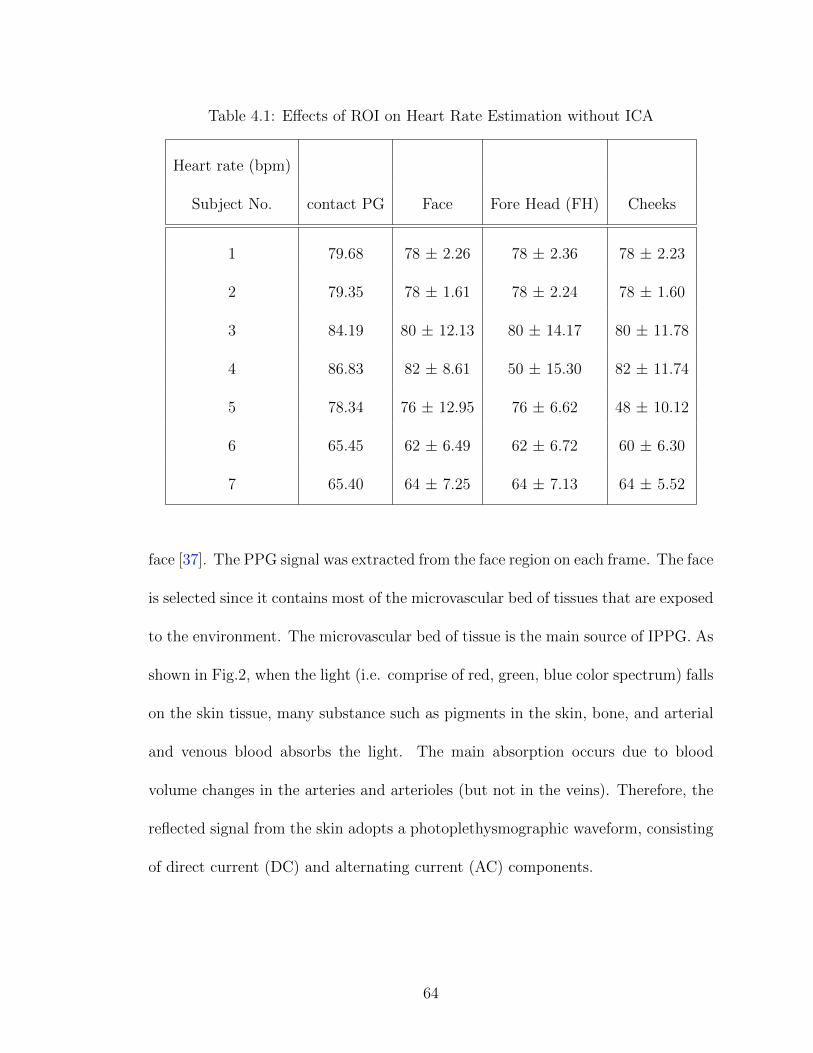
The second part of thesis refers to the study of image photoplethysmogra-

phy (IPPG), a cost-effective and flexible method for heart rate monitoring using

videos recorded in ambient light. We use low-cost commercial grade video record-

ing equipment (mobile camera/Digital camera) with an ambient light source. The

study includes information about signal processing algorithms for estimating heart

rate, relevant parameters, and comparison with standard techniques. Such low-cost,

multi-purpose solutions for quick screening of subjects provides us with sensible and

useful information on elevated body temperature and heart rate. Hence, these meth-

ods show promising results that enable mass fever screening as a possibility through

temperature and heart rate monitoring, where low cost of installation and flexibility

are important.

IR THERMOGRAPHY(IRTG) AND IMAGEPHOTOPLETHYSMOGRAPHY(IPPG) : NON-CONTACT

MEDICAL COUNTER MEASURES FOR INFECTIONSCREENING

by

Yedukondala Narendra Dwith Chenna

Thesis submitted to the Faculty of the Graduate School of theUniversity of Maryland, College Park in partial fulfillment

of the requirements for the degree ofMaster of Science

2017

Advisory Committee:Professor Dr. Rama Chellappa, Chair/AdvisorProfessor Dr. Behtash BabadiDr. Quanzeng Wang

c© Copyright byYedukondala Narendra Dwith Chenna

2017

Acknowledgments

I owe my gratitude to all the people who have made this thesis possible and

because of whom my graduate experience has been one that I will cherish forever.

First and foremost I’d like to thank my advisor, Professor Dr. Rama Chel-

lappa and my mentor Dr. Quanzeng Wang for giving me an invaluable opportunity

to work on challenging and extremely interesting projects. It has been a pleasure to

work with and learn from such extraordinary people. I would also like to thank my

co-advisor, Dr. Behtash Babadi for his support. My colleagues at the Optical Diag-

nostics laboratory at Food and Drug Administration (FDA) have enriched my grad-

uate life in many ways and deserve special mention. Phejhman Ghassemi helped me

throughout this study including assistance with setting up experiments/laboratory

protocols setup and analysis of measurements. My interactions in team meetings

with Joshua Pfefer and Jon Casamento have also been very fruitful.

I owe my deepest thanks to my family - my mother and father who have always

stood by me and guided me through my career, and have pulled me through against

impossible odds at times. Words cannot express the gratitude I owe them.

My friends here at University of Maryland have been a crucial factor, without

whom the thesis would have been complete one month earlier. A special thanks goes

to my friends here at College Park: Shankar, Koutilya, Goutham, Harsha, Harika,

Abhinay, Surya, Navaneeth, Dayal , Raghu and others for making my graduate study

enjoyable and memorable. Special thanks to Pallavi and Soumya for the reviews and

edits during the initial draft. A special mention to my archrival, Deepika, for the

ii

discussions on image registration, she was a great motivation and company.

I’d like to express my gratitude for their friendship and support. I would like to

acknowledge financial support for Research Fellowship from Oak Ridge Institute for

Science and Education (ORISE). It is impossible to remember all, and I apologize

to those I’ve inadvertently left out.

Lastly, thank you all and thank God!

iii

Table of Contents

List of Figures vi

List of Abbreviations viii

1 Introduction 11.1 Overview . . . . . . . . . . . . . . . . . . . . . . . . . . . . . . . . . . 11.2 Contributions of Thesis . . . . . . . . . . . . . . . . . . . . . . . . . . 31.3 Outline of Thesis . . . . . . . . . . . . . . . . . . . . . . . . . . . . . 4

2 Theory 62.1 Infrared Thermography (IRTG) . . . . . . . . . . . . . . . . . . . . . 62.2 Image Photoplethysmography (IPPG) . . . . . . . . . . . . . . . . . . 8

3 IR Thermography (IRTG) 123.1 Image Registration . . . . . . . . . . . . . . . . . . . . . . . . . . . . 12

3.1.1 Nature of Registration . . . . . . . . . . . . . . . . . . . . . . 133.1.2 Image Modality . . . . . . . . . . . . . . . . . . . . . . . . . . 143.1.3 Similarity Metric . . . . . . . . . . . . . . . . . . . . . . . . . 143.1.4 Transformation Model . . . . . . . . . . . . . . . . . . . . . . 18

3.1.4.1 Demons Registration . . . . . . . . . . . . . . . . . . 213.1.4.2 Spline Registration . . . . . . . . . . . . . . . . . . . 233.1.4.3 Interpolation . . . . . . . . . . . . . . . . . . . . . . 26

3.1.5 Optimization . . . . . . . . . . . . . . . . . . . . . . . . . . . 283.2 Implementation: Thermal and Visible Image Registration . . . . . . . 30

3.2.1 Coarse Registration . . . . . . . . . . . . . . . . . . . . . . . . 313.2.2 Fine Registration . . . . . . . . . . . . . . . . . . . . . . . . . 32

3.3 Results and Analysis . . . . . . . . . . . . . . . . . . . . . . . . . . . 363.3.1 Registration Accuracy . . . . . . . . . . . . . . . . . . . . . . 363.3.2 Canthi Temperature Measurement . . . . . . . . . . . . . . . 42

iv

4 Imaging Photoplethysmography (IPPG) 504.1 Overview . . . . . . . . . . . . . . . . . . . . . . . . . . . . . . . . . . 504.2 Implementation/Methods . . . . . . . . . . . . . . . . . . . . . . . . . 52

4.2.1 Experimental Setup . . . . . . . . . . . . . . . . . . . . . . . . 524.2.2 Signal Extraction . . . . . . . . . . . . . . . . . . . . . . . . . 534.2.3 Heart Rate Estimation Algorithm . . . . . . . . . . . . . . . . 53

4.2.3.1 Independent Component Analysis . . . . . . . . . . 564.2.4 Pulse Amplitude Mapping . . . . . . . . . . . . . . . . . . . . 58

4.3 Results and Analysis . . . . . . . . . . . . . . . . . . . . . . . . . . . 594.3.1 Heart Rate Measurement from Face Region . . . . . . . . . . 634.3.2 Heart Rate Measurement from Fore Head Region . . . . . . . 654.3.3 Heart Rate Measurement from Cheek Region . . . . . . . . . 65

5 Conclusion 725.1 IR Thermography . . . . . . . . . . . . . . . . . . . . . . . . . . . . 725.2 Image Plethysmography . . . . . . . . . . . . . . . . . . . . . . . . 73

A Results Analysis 75A.1 Bland-Altman Analysis . . . . . . . . . . . . . . . . . . . . . . . . . . 75A.2 Recall Graphs . . . . . . . . . . . . . . . . . . . . . . . . . . . . . . . 75

Bibliography 77

v

List of Figures

2.1 Thermal image : temperature drift after auto-adjustment . . . . . . . 72.2 Temperature accuracy based on various sources of uncertainty . . . . 72.3 Canthi regions for fever screening . . . . . . . . . . . . . . . . . . . . 92.4 The canthi regions for fever screening (a: an IR image; b: a white-

light image) . . . . . . . . . . . . . . . . . . . . . . . . . . . . . . . . 92.5 Absorption spectrum of Hemoglobin within 450 nm to 700 nm wave-

length range . . . . . . . . . . . . . . . . . . . . . . . . . . . . . . . . 11

3.1 Joint histograms for measuring registration accuracy using MutualInformation (a) Mis-aligned Images (b) Ideally Registered Images . . 17

3.2 B-spline mesh grid control points . . . . . . . . . . . . . . . . . . . . 243.3 B-spline basis function . . . . . . . . . . . . . . . . . . . . . . . . . . 263.4 Forward warping method for spatial transformation . . . . . . . . . . 283.5 Backward warping method for spatial transformation . . . . . . . . . 293.6 Block diagram of the two-step registration strategy . . . . . . . . . . 313.7 Block diagram of Image Registration . . . . . . . . . . . . . . . . . . 323.8 Input IR and visible Images after coarse registration and ROI Selection 333.9 Edge maps for IR and visible images after ROI Selection . . . . . . . 343.10 Image Registration using edge maps after: (a) Affine (b) Demons

registration . . . . . . . . . . . . . . . . . . . . . . . . . . . . . . . . 343.11 Registered images using checkered view (a: coarse registration; b:

fine registration) . . . . . . . . . . . . . . . . . . . . . . . . . . . . . 363.12 Images from three cameras (a: IRT1; b: IRT2; c: visible camera) . . . 373.13 Control point selection for registration evaluation (a: IR image; b:

visible image) . . . . . . . . . . . . . . . . . . . . . . . . . . . . . . . 383.14 Control point selection in eye region for registration evaluation (a: IR

image; b: visible image) . . . . . . . . . . . . . . . . . . . . . . . . . 383.15 Qualitative comparison of image registration using affine, Demons

and cubic BSpline model (Face Region) . . . . . . . . . . . . . . . . . 403.16 Qualitative comparison of image registration using affine, Demons

and cubic BSpline model (Face Region) . . . . . . . . . . . . . . . . . 40

vi

3.17 Qualitative comparison of image registration using affine, Demonsand cubic BSpline model (Face Region) . . . . . . . . . . . . . . . . . 41

3.18 Qualitative comparison of image registration using affine, Demonsand cubic BSpline model (Eye Region) . . . . . . . . . . . . . . . . . 41

3.19 Qualitative comparison of image registration using Affine, Demonsand cubic BSpline model (Eye Region) . . . . . . . . . . . . . . . . . 43

3.20 Qualitative comparison of image registration using affine, Demonsand cubic BSpline model (Eye Region) . . . . . . . . . . . . . . . . . 44

3.21 Temperature measurement (a) Fore Head (FH) (b) Left Canthi (LC)and (c) Right Canthi (RC) . . . . . . . . . . . . . . . . . . . . . . . . 44

3.22 Figure with caption indented . . . . . . . . . . . . . . . . . . . . . . . 453.23 FLIR Temperature measurement (a) Fore Head (FH) (b) Left Canthi

(LC) and (c) Right Canthi (RC) . . . . . . . . . . . . . . . . . . . . 453.24 Bland Altman - ICI Temperature measurement (a) Fore Head (FH)

(b) Left Canthi (LC) and (c) Right Canthi (RC) . . . . . . . . . . . . 463.25 Bland Altman - FLIR Temperature measurement (a) Fore Head (FH)

(b) Left Canthi (LC) and (c) Right Canthi (RC) . . . . . . . . . . . . 463.26 land Altman - ICI Temperature measurement in Fore Head (FH) . . . 473.27 Bland Altman - ICI Temperature measurement in Left Canthi (LC) . 473.28 Bland Altman - ICI Temperature measurement in Right Canthi (RC) 49

4.1 Red, Green and Blue Channel indicating Normalized pixel values usedto estimate heart rate . . . . . . . . . . . . . . . . . . . . . . . . . . . 54

4.2 Heart rate frequency Spectrum within (0.75,4) Hz frequency range . . 554.3 Heart rate frequency Spectrum within (0.75,4) Hz frequency range . . 564.4 Pulse Amplitude Map at Heart rate frequency with 50x50 grid size . 614.5 Pulse Amplitude Map at Heart rate frequency with 25x25 grid size . 614.6 Pulse Amplitude Map at Heart rate frequency with 10x10 grid size . 624.7 Heart rate estimation (a) ROI Selection (b) Time Series signal and

(c) Frequency Spectrum . . . . . . . . . . . . . . . . . . . . . . . . . 634.8 ROI Selection for IPPG - Face Region . . . . . . . . . . . . . . . . . 664.9 ROI Selection - Fore Head Region . . . . . . . . . . . . . . . . . . . 664.10 ROI Selection - Cheek Region (Lower Face) . . . . . . . . . . . . . . 70

vii

List of Abbreviations

MMIR Multi-Modal Image RegistrationMI Mutual InformationLC Left CanthiRC Right CanthiFH Fore HeadSD Standard DeviationFFD Free Form DeformationIRTG Infrared ThermographIPPG Image PhotoplethysmographyCC Correlation CoefficientSSD Sum of Squared DifferencePPG Photo PlethysmographyWHO Word Health OrganizationICA Independent Component AnalysisJADE Joint Approximation Diagonalization of Eigen matrices

viii

Chapter 1: Introduction

1.1 Overview

According to an estimate from World Health Organization (WHO), pandemic

from viruses like Ebola, H5N1 bird flu could kill upto 100 million people [2]. Mitigat-

ing threat of such infectious pandemics may be possible through mass fever screening

in public places such as airports, hospitals and border crossing points [7, 12]. Fever

is one of the common diagnostic symptoms, which can be used to contain the epi-

demic through isolation of patients and medical care. In case of infectious diseases

outbreak, a quick and efficient fever screening process is needed to identify infected

patients. Early symptoms of infections can be detected through abnormalities in

body temperature and heart rate. Conventional methods for measuring such human

vital signals is invasive, time consuming and labor intensive [34,44]. To enable mass

fever screening we need devices/methods that are non-invasive, cost-effective, easy

to install and be able to detect patients with fever [29]. Several studies [18] show that

IRTGs enable a viable and non-invasive mass screening approach through detection

of elevated temperatures. IRTGs have been used successfully as a tool for mass fever

screening of SARS-2003 outbreak [29,30]. Research in this area is necessary as epi-

demics like ebola, bird flu, zika are expected to hit 20 to 30 % of world’s population.

1

International Organization for Standardization (ISO) meeting in 2005 at IEC-DIN

Germany, discussed Standard Technical Reference [29, 40] to enable acceptance of

infrared imaging in medical applications. Fever screening through IRTGs for hu-

man body temperature measurement requires identification of effective site for such

measurement [30]. The regions medically adjacent to inner canthi are preferred sites

for such fever screening based on temperature measurement (IEC/ISO 2008) [30].

This thesis tries to automate the process of temperature measurement using ther-

mograms. Accurate localization of canthi regions is possible on visible light images,

which are rich in features. Multi-modal image registration (MMIR) of thermal and

visible images enables canthi localization in thermal images. Registration of multi-

modal images from visible and IR face images is well studied in the literature on

face recognition [21]. Accuracy of registration is studied in the context of canthi

detection and the feasibility of automatic canthi-based temperature measurement

as an alternative for manual measurement.

Similarly, recent techniques of IPPG investigate use of cost effective methods

of heart rate monitoring using recorded video of the subject. This enables contact-

free measurement of human vital signals at a distance from the subject, which is very

appealing for mass fever screening application. These passive imaging methods en-

able long term monitoring of vital signals without any inconvenience to the patients.

Studies include background information about signal processing algorithms for es-

timating heart rate, relevant parameters and comparison with standard techniques.

Such low-cost, multi-purpose solutions for quick screening of subjects provide us with

sensible and useful information about body temperature and heart rate. Abnormal-

2

ities in body temperature and heart rate are clear indicators of infection. These

measurements can be used for screening such infected subjects. These recent devel-

opments in research show promising results that enable us to use consumer grade

electronics as cost effective diagnostic tools for evaluation of body temperature or

heart pulse rate through thermograms and recorded videos respectively. This thesis

studies techniques of image registration to enable automatic IRTG-based tempera-

ture measurement and the feasibility of heart rate monitoring through commercial

video recording equipment. The study evaluates influence of different parameters

on performance of these methods along with experimental results.

1.2 Contributions of Thesis

This thesis explores different methods for registration of visible and IR face im-

ages to enable temperature measurement using inner canthi. Especially for a human

face, which is non-rigid, affine models are limited in accuracy for registration. We

implement a free form deformation (FFD)-based registration method to improve the

registration accuracy after affine transformation. The improvement in registration

accuracy using affine and deformable transformations is compared. We also evalu-

ate the feasibility of registration-based automatic temperature measurement as an

alternative to manual measurement. A complete implementation for registration

of visible and IR images through affine and deformable transformations in MAT-

LAB (The MathWorks. Inc.) is provided. In conclusion, we compare the manual

canthi-based temperature measurement against automated image registration based

3

method.

Moreover, the study investigates the use of low-cost (mobile camera/Digital

Camera) video recording equipment in ambient light for non-contact heart rate

estimation. The recorded video using RGB color space with webcam/mobile cam-

era shows heart rate pulsations in green channel which shows highest absorption.

Changes in ambient light and automatic brightness adjustment in such video record-

ing devices have significant influence on the underlining PPG signal. The study

relies on manual segmentation to analyze different ROIs for heart rate estimation.

We validate the performance characteristics through mean error, standard deviation

of error, root mean square error (RMSE) along with Bland-Altman and correlation

analysis. The thesis also studies the influence of different parameters like region of

interest (ROI), window size for spectrum analysis and frame rate. This enables us

to outline the requirements and their influence on heart rate estimation using IPPG.

1.3 Outline of Thesis

The thesis is organized as follows. Chapter 2 gives background information

on IR thermography (IRTG) and image photoplethysmography (IPPG). Chapter

3 gives an introduction to image registration and its application in the context of

IR Thermography. It discusses the implementation details of thermal to visible

image registration and canthi temperature measurement along with results for mea-

surement error analysis. Chapter 4 describes the experimental setup, input videos,

overview of IPPG algorithm and results for heart rate estimation. Chapter 5 gives

4

conclusions drawn from experimental results.

5

Chapter 2: Theory

2.1 Infrared Thermography (IRTG)

IR cameras produce images to indicate temperature information from a sur-

face. Thermography is a passive, non-contact imaging method that is cost-effective,

quick and does not inflict any pain on the patient. The object surface temperature

under observation governs the amount of IR radiation emitted from the surface. In

case of fever screening, IR imaging is a non-invasive physiological test where the

camera can be placed at a distance from the subject to be screened. Electrical sig-

nals generated by IR cameras are proportional to the IR radiations emitted from

human skin [29], which are used to display temperature profile graphically. The im-

age pattern indicates the inflammations (hot regions) and nerve dysfunction (cold

regions). The observed temperature reading on human skin are below the typical

body temperature of 37 ◦C due to heat evaporation, conduction and convection

principles. The measured skin temperature, is a function of internal organ, heat

properties of tissues and heat emissivity of skin. These features enable IR thermo-

grams to be used for early identification or screening of individuals with elevated

temperature as a first sign of infection [12]. In general, the setup for thermal imag-

ing requires a stable indoor environment with stable ambient temperature (20 to

6

Figure 2.1: Thermal imaging temperature drift after auto-adjustment [30]

Figure 2.2: Temperature accuracy based on various sources of uncertainty [30]

25 ◦C) and stability of +/- 1 ◦C, with a relative humidity ranging from 40 % to

75 %. Based on the type of IR imaging, they have different degrees of temperature

drift depending on self-correlation (Fig.2.1), uniformity within field of view, mini-

mum detectable temperature difference, error and stability of threshold temperature

(Fig.2.2), distance effect and detector sizes. An external black-body maintained at

given temperature is used as a reference to correct the thermograph for any drift in

temperature sensitivity. This enables satisfactory repeatability of the temperature

measurement. The temperature readings from the camera are calibrated based on

the measurement from the black body used as a temperature reference.

7

Many other factors that influence temperature measurement include : pa-

rameters of IR imaging system, variation in operating environment and screened

subjects. These variations might lead to false-negative readings which will strongly

undermine the effectiveness of the screening process. Hence, a reliable and scientific

method for accurately estimating the body temperature is essential for success-

ful implementation of such mass fever screening methods. A recent research [30],

studied different regions on IR face images that show good correlation with body

temperature. The IEC 80601-2-59:2008 international standard indicates that the

canthi regions (Fig.2.3) provide accurate estimates of core body temperature, since

the canthi regions are supplied by the internal carotid artery and are less suscepti-

ble to external environmental changes. Anatomically these regions are adjacent to

inner corner of the eye and vary in size from subject to subject. Therefore, rapid,

automated identification of the canthi regions (Fig.2.4) within facial IR images may

greatly facilitate fever screening. Automatic localization of canthi in thermal images

is achieved through MMIR of thermal and visible images, followed by fiducial point

detection [4] in visible face images to localize the canthi regions. The canthi regions

on thermal face images are used to measure temperature and compare its feasibility

with manually obtained temperature measurement.

2.2 Image Photoplethysmography (IPPG)

Plethysmography steams from Greek work plethysmos meaning variations in

size owing to blood circulation. Conventional plethysmography measures pulsativ-

8

Figure 2.3: Canthi regions for fever screening (IEC 80601-2-59:2008) [1]

Figure 2.4: The canthi regions for fever screening (a: an IR image; b:a white-light image) [9]

ity in tissue volume and blood profusion directly through strain gauge. The gold

standard currently for measurement of cardiac pulses is through electrocardiogram

(ECG). It requires patient to wear adhesive gel patches or chest straps, which can

cause skin irritation or discomfort. The commercially available pulse-oximetry,

which are generally attached to fingers or ear lobes are inconvenient for subjects

and can cause pain over long duration. Availability of a remote and non-contact

based monitoring or screening systems for cardiovascular activity is an interesting

prospect for primary health care and surveillance. Pavlidis et. al. [17] demonstrated

an approach for measuring of physiological parameters through face and thermal

videos. Photo Plethysmography (PPG) is a low-cost and non-invasive means of

sensing cardiovascular pulse by measuring the variation in transmitted or reflected

9

light through tissues [38]. Such methods may not provide the details of cardiac elec-

trical conduction as in ECG, but they give useful information on heart pulse rate by

acquiring short duration videos in an unobstructed and comfortable manner. Typi-

cally, conventional PPG has a dedicated light source, which can be broadly classified

into two types: Transmission mode PPG and Reflectance mode PPG. Transmission

mode PPG measures how light is obstructed and absorbed through tissues using an

LED light source on one side and a photodetector on the other. Reflectance mode

PPG has the LED and photodetector on the same side and studies the amount of

light reflected from a tissue surface. The underlying PPG signal in such plethysmo-

graphs is a complex function of physiological parameters, measurement methodology

and physical properties of sensor.

Non-contact image PPG (IPPG), is a type of reflectance mode PPG which

uses video recordings with ambient light sources. It is an active field of research, of-

fering insights into implementation of non-invasive human vital sign monitoring [42].

The basic principle of IPPG relies on interaction of ambient light with biological

tissues. Similar to conventional PPG signals, it is a complex function of physiologi-

cal parameters, acquisition system and the properties of light scattering. The light

interactions with biological tissues results in intensity modulation in the recorded

video which is synchronous with heart beat. There are many intrinsic components

that influence these fluctuation in intensities like blood volume, blood-vessel-wall

movement and the orientation of the red blood cells. One of the main contrib-

utors of such variations is blood flow and volumetric change in blood-vessel due

to movement of blood stream. The absorption spectrum within color spectrum for

10

Figure 2.5: Absorption spectrum of Hemoglobin within 450 nm to 700nm wavelength range [49]

wavelength span of 450-700 nm for (1) oxyhemoglobin (HbO2) and (2) deoxygenated

hemoglobin (Hb) as shown in Fig. 2.5. The green light shows peak absorption and

red shows the lowest absorption, which is validated based on observations from ex-

perimental results. Such non-invasive assessements of cardiovascular activity are

useful in surveillance to estimated abnormalities in heart pulse rate.

11

Chapter 3: IR Thermography (IRTG)

3.1 Image Registration

Image registration is fundamental to a wide range of applications in medical

imaging. Image registration can be modeled as a transformation that defines a

spatial correspondence between two images. It is the process of spatially aligning

two or more images captured using various modalities and at different viewing angles

and time instants. Registration methods can be broadly classified as follows [23]:

I. Nature of Registration : (i) Extrinsic and

: (ii) Intrinsic

II. Image Modality : (i) Uni-modal and

: (ii) Multi-modal

III. Similarity Metric : (i) Landmark based and

: (ii) Intensity based

IV. Transformation Model : (i) Rigid

: (ii) Affine and

: (iii) Deformable

12

3.1.1 Nature of Registration

Based on the nature of registration, registration methods can be classified into

extrinsic and intrinsic methods. Extrinsic methods use artificial objects, which are

either placed within the field of view or attached to the subject, while capturing the

image. These objects are designed to be easily detectable in two or more images

(which are) to be registered and are used for estimating the spatial transformation

for registration. Extrinsic object based registrations are relatively fast and enable

automation. However, these methods are limited due to constraints on the provision

of such objects under different conditions, additional cost and advanced planning

before image capture. This model does not use any information from the subject

and is mostly limited to rigid transformation.

Intrinsic methods use information from a subject image, the transformation is

based on identifiable features from the images to be registered. Intrinsic methods can

be broadly classified into (a) Landmark-based and (b) Intensity-based approaches.

Landmark-based registration uses features points identified in different images and

determines the transformation based on these feature points, which are easy to

locate by the user or automated algorithm. Landmark-based methods are generally

used to define rigid or affine transformations. If the number of feature points is

large enough more complex deformable transformations can be estimated. The

search for optimum transformation is simplified due to sparse landmark points,

which greatly speeds up the registration process. Nonetheless, it usually requires

user interaction for the landmark selection, which limits its applications. Intensity-

13

based methods use the intensity values of pixels. These methods enable flexibility

for applications with similar or different modality images and can be adapted to

most type of transformations. However, these methods are limited in application

due to computational complexity of registration.

3.1.2 Image Modality

The registration method can be classified into two types based on modality

of images involved : (a) mono-modal image registration and (b) Uni-modal image

registration (MMIR) [24]. In uni-modal registration, the images to be registered

have been acquired using similar sensors, but from different view points, or times

or scales. Uni-modal registration is quite widely used in growth monitoring, com-

parison, subtraction imaging, and many other applications. In case of MMIR, the

images to be registered are obtained using different sensors. MMIR of images pro-

vides complementary information, which uses comparison of spatial points for useful

information about infection or disease.

3.1.3 Similarity Metric

Similarity metric is used to define a qualitative metric for alignment of the

images to be registered. The registration algorithm tries to minimize/maximize

the similarity metric to achieve spatial alignment of images. Similarity Metric is

crucial in the image registration algorithm. It determines the accuracy, robustness

and flexibility of registration algorithms. These measures can be broadly classified

14

into: landmark-based and intensity-based measures. Landmark-based methods use

unique landmarks in both the reference and moving images, which can be used

to estimate the transformations. Landmarks can provide a basis for Rigid/affine

transformation. Alternative includes extraction of feature points in one image and

matching them in another image. Intensity-based methods work directly with pixel

intensity level. However, intensities obtained with different modalities do not show

a linear relation. Other methods that do not rely just on intensity value, but try to

model the correlation are better suited for MMIR. Intensity based metrics widely

used in MMIR for medical images, include Sum of Squared Difference (SSD) [24],

Normalized Cross Correlation (NCC) [24], Correlation Ratio (RC) [24] and Mutual

Information (MI) [24]. In this section we will briefly discuss SSD, NCC and MI

methods, which are quite widely used in medical image registration. Simplest mea-

sure for the similarity of images is based on the SSD between images Ireg and Imov

with transformation T (x, y) given by:

ISSD =∑

[Imov(T (x, y))− Ireg(x, y)]2 (3.1)

This measure is used for images with similar modality, which is optimal if

images with white Gaussian noise are aligned. A more general approach assumes

a linear relationship between image intensities. In such a case similarity between

images Ireg and Imov can be expressed using NCC

INCC =

∑(Ireg(x, y)− µref )(Imov(T (x, y)− µmov)√∑

(Ireg(x, y)− µreg)2∑

(Imov(T (x, y))− µmov)(3.2)

15

Where the images are corrected with µreg and µmov representing mean im-

age intensity. This metric is more flexible than SSD, nevertheless it is restricted to

mono-modal registration. Mutual Information as a metric for image registration was

first proposed by Woods et al . [48]. In case of MMIR, regions with certain intensity

level in an image would correspond to similar regions in another image that contain

a similar intensity level distribution (maybe of different value). Ideally, the corre-

spondence between these intensity level distribution might not change significantly

across different images. Hill et al. [13] proposed registration by constructing a joint

histogram, which is a two-dimensional plot showing combinations of grey values as

shown in Fig.3.1. Location (i, j) in the joint histogram corresponds to a count of the

values with intensity ’i’ in the first image and intensity ’j’ in the second image. The

joint histogram shows increased dispersion as the misalignment of images increases.

Shannon entropy (also referred to as entropy) [24] is used as a registration metric

to measure dispersion in the joint histogram. Entropy of a discrete random variable

Xi with probability distribution function pi is given by [24]:

H(X) = −∑

pi(log2(pi)) (3.3)

Entropy does not depend on the value of a random variable, but depends

on the distribution of the random variable. This definition of entropy can be ex-

tended to images, where the probability distribution function is constructed using

the histogram distribution of pixel values in the image. Entropy of a joint histogram

decreases with better alignment of the images as shown in Fig.3.1. Define MI as

16

Figure 3.1: Joint histograms for measuring registration accuracy us-ing Mutual Information (a) Mis-aligned Images (b) Ideally RegisteredImages

IMI based on the entropy of two input images A and B, which relates to the joint

histogram entropy as follows:

IMI = H(A) +H(B)−H(A,B) (3.4)

Where H(A), H(B) and H(A,B) are the entropy’s of image A, image B and

the joint histogram, respectively. The above equation relates the minimization of

the joint histogram to the maximization of MI. Hence, the problem of registration is

converted into an optimization problem that tries to maximize the MI using different

transformations.

17

3.1.4 Transformation Model

Transformation Model is one of the key problems in image registration. The

transformation model used in registration defines how the coordinates of two images

are related. These models can be broadly classified into global and local transfor-

mation models. Global transformation is applied to the whole image, whereas local

transformations are applied to each pixel or group of pixels in the image. Global

transformations are quite widely used because of their simplicity in estimating few

parameters. Simple translation and rotation motion of a planar object can be de-

fined as a rigid transform. Affine transformation allows scaling and shear in addi-

tion to the rigid transform. Local transformations are used to model registration of

non-planar surfaces, where the motion or registration cannot be modeled by global

parameters. A generic transformation can be defined as a combination of global and

local transformations:

T (x, y) = Tglobal(x, y) + Tlocal(x, y) (3.5)

Consider two images Iref and Imov, which represent reference and moving im-

ages, respectively. The transformation T is applied on the moving image and mea-

sures the similarity metric. The optimization process tries to minimize/maximize

the similarity metric over all possible parameters of the transformation. Let Ireg

denote the registered image. The goal is to find T (or equivalently its inverse) which

provides a mapping from Imov to Ireg.

18

The relation between Ireg and Imov can be defined as follows:

Ireg(T (x, y)) = Imov(x, y) (3.6)

Where T is a transformation defined by a global and a local transformation.

The goal is to estimate T , that maximizes/minimizes the similarity metric. Transfor-

mation (T ) is defined on the image coordinates of the moving image Imov transform-

ing it to Ireg, which try to match the Iref image coordinates. The global transforma-

tion (Tglobal) is the product of geometric transformations, which includes translation,

rotation, scaling and skew as shown below:

Tglobal =

1 0 tx

0 1 ty

0 0 1

α −β 0

β α 0

0 0 1

1 k 0

0 1 0

0 0 1

Sx 0 0

0 Sy 0

0 0 1

(3.7)

tx, ty = Translation of the image in the x and y direction

θ = angle measured in the counter clockwise direction from the x− axis, (α =

cos(θ), β = sin(θ))

k = shear factor along the x− axis

Sx, Sy = change in scale in the x and y direction

A Local transformation improves the registration accuracy for non-planar sur-

faces. However, the large number of parameters to be estimated and high compu-

tational complexity limits its application. Deformable registration is used to model

19

non-planar transformations locally displace a moving image Imov as shown in eq.3.8.

These registration models offer higher degrees of freedom to represent the transfor-

mation. This enables modelling of local deformation more accurately resulting in

high accuracy registration. Free Form Deformations (FFDs) are well studied non-

rigid models used to describe more general deformations for each pixel or a group of

pixels with high degrees of freedom and with smoothness constraints in the defor-

mation. FFDs can be broadly classified into parametric and non-parametric trans-

formations. The parametric transformations are defined on a coarse grid of control

points, where the transformation is parametrized by basis functions. In contrast,

non-parametric transformations have a dense set of displacement vectors associated

with every pixel in the image. Such algorithms are used to describe more general

deformations for each pixel with a high degrees of freedom, along with smoothness

constraints. In case of parametric transforms, where T is expressed as the displace-

ment field (u, v) on a coarse grid of control points, as in eq.3.8. The transformations

are required to be smooth and invertible. In case of non-parametric FFDs like

demons algorithm, it includes an additional smoothness constraint on transforma-

tion using the weighted Gaussian function. These transformations require a great

deal of computation time, which can be improved through numerical algorithms and

coarse-to-fine registration strategy. The parametrized and non-parametrized algo-

rithms can be defined as displacement vectors for moving image Imov(x, y) with a

transformation as follows.

20

T (x, y) = (x+ f(u), y + f(v)), (3.8)

where u and v are vertical and horizontal displacement fields, f is the basis

function used to define the transformation. Given a pair of images Iref and Imov

which are used to simultaneously recover u and v. A weighted blend of these dis-

placement field from neighborhood is used to determine the displacement of a pixel

in the image. The blending weights are determined by a weighted Gaussian function

and cubic B-splines for demons algorithm and Spline registration, respectively. The

displacement vectors in case of Cubic B-spline registration at each pixel is defined

as a combination of B-spline basis functions, which themselves provide smoothness

constraints on the transformation.

3.1.4.1 Demons Registration

Demons Algorithm [43] proposed deformable registration as a diffusion process,

which introduces entities called Demons that exerts forces according to the local

characteristics of the images. These forces were inspired from optical flow equations

[14]. It can be considered as a type of viscous fluid model-based registration. The

basic idea of the Demons algorithm for deformable registration is that the reference

image acts as a local displacement vectors that moves the pixels in the moving

image to match the reference image. During each iteration, the moving image is

transformed using the moving vector dV = (dx, dy) for each pixel as shown in eq.

3.8 [11]:

21

dV (n+1) =(I(n)mov − I

(0)ref )(∇I(0)ref )

(I(n)mov − I(0)ref ) + |∇I(0)ref |

(3.9)

Where I(n)ref and I(n)mov are the intensities of reference and moving images, re-

spectively, at the nth iteration. I(0)ref and I(0)mov represent the original reference and

moving images, respectively. A Gaussian filter is used to smooth the displacement

fields, which suppresses noise and preserves the geometric continuity of the deformed

image. This algorithm can be efficiently implemented using using convolution op-

eration, which enables its application to registration problems which require high

dimensions. The gradient of the reference image ∇I(0)ref is computed only once for all

the iterations. Moreover, the Demons algorithm assumes that the displacement vec-

tor is reasonably small or local. However, in real clinical cases, such an assumption

may be violated. To reduce the magnitude of displacement vectors, the multi-scale

approach is used, where both reference and moving images are down-sampled to

low resolution images using Gaussian pyramid scaling. The displacement fields at

each stage are up-sampled from a low resolution scale to a higher resolution scale.

This provides a significant computational advantage for large image sizes. However,

the conventional Demons algorithm is applicable only to uni-modal image registra-

tion [35,50]. In this study, the edge maps for IR and visible images generated using

a canny edge detector are used for estimating FFD registration using Demons al-

gorithm. These edge maps emphasize on the contour edges of face and eyes, which

show a good similarity between thermal IR and visible images [22]. The contours

in eye regions are used to predict the free-form transformation used for non-rigid

22

registration. Iterative optimization method uses an effective stopping criteria, a tol-

erance criterion that stops the iterations if the SSD in intensity value increases with

each iteration and also if the decrease in the similarity metric for each iteration is

within a convergence tolerance.

3.1.4.2 Spline Registration

Spline-based registration models are among the most common and important

transformation models used for deformable registration in medical imaging. Spline-

based registration algorithms use coarse grid of control points from the moving

image and a spline basis function that defines the transformation in the neighbor-

hood of these points. The spline based registration can be divided into two types

: (a) thin-plate splines and (b) B-spline. Thin-plate splines have a global influence

on the transformation. In contrast, B-splines are only defined in the neighborhood

of control points. Any perturbation in control points influences points within the

neighborhood of that point. This makes B-spline based registration a computation-

ally efficient tool for deformable registration. Cubic B-spline based FFDs deform

an object by manipulating the underlying mesh of control points. The vector fields

(ui,vi), represent the dense displacement fields estimated as two dimensional splines

controlled by a small number of control points (Uj,Vj) highlighted in red as shown in

Fig.3.2. The spline imposes an implicit smoothness on the motion fields, eliminat-

ing the need for additional smoothness constraints, in many instances. To define a

spline based FFD, defined on mesh of nx by ny control points with uniform spacing.

23

Figure 3.2: B-spline mesh grid control points

The ui and vi defines the displacement vectors at each pixel given by:

ui = u(xi, yi) =∑UjBj(xi, yi) =

∑Ujwij (3.10)

Where Bj(xi, yi) are called basis functions and are non-zero over a small in-

terval. wij = Bj(xi, yi) weights that are used to emphasize that (ui, vi) are known

linear combination of (Uj, Vj) control points.

Implementation of B-spline makes the spline control grid on a regular grid of

sampling points (Xj, Yj) = (mxi,myi), so that each set of mxm pixels corresponds to

a single spline patch. The basis functions are spatially shifted versions i.e. Bj(x, y) =

B( (x−Xj)

m, (y−Yj)

m). Fig.3.3 visualizes four different types of basis functions:

24

I. Block : B(x,y)=1 on [0,1][0,1]

II. Linear : (1-x-y) on [0,1][0,1]

: (x+1) on [-1,0][0,1]

: (y+1) on [0,1][-1,0]

III. Quadratic : B2(x)B2(y) on [-1,1][-1,1]

where B2(x), B2(y) are second order (quadratic) B-Spline

IV. Cubic : B3(x)B3(y) on [-1,1][-1,1]

where B3(x), B3(y) are third order (cubic) B-Spline

B-splines are locally controlled, which makes them computationally efficient.

The basis functions of cubic B-spline have a limited support, changing the control

point affects the transformation only in the local neighborhood of control point. The

control points’ resolution determines the number of degrees of freedom and conse-

quently the computational complexity. A large spacing between control points allows

modeling of global non-rigid deformations, while a small spacing between control

points allows modeling of highly local deformations. In the multi-scale approach,

the spacing between control points decreases from a lower resolution to higher res-

olution, which increases the resolution of control mesh. At each level of resolution,

the control mesh and associated spline-based FFD defines a local transformation.

To avoid the overhead of calculating several B-spline coefficients separately, the local

transformation defined by a single B-sline whose control point mesh is progressively

refined. The control point mesh at level L is refined by inserting new control points

to create the control point mesh at level L+1. The number of horizontal and ver-

tical control points double every step. The spline-based FFD transformation can

25

Figure 3.3: BSpline basis functions

be smoothed by introducing a penalty regularization term. The MIRT [3] tool used

for cubic B-spline registration uses curvature regularization based on discrete cosine

transformation (DCT) [10], to yield a stable and fast implementation.

3.1.4.3 Interpolation

At each iteration of registration, the optimizer determines the parameter of

the transformation (T ) that will be applied to the moving image, also called image

warping. Image warping is defined as the process of transforming the moving image

using the estimated transformation. Irrespective of the type of transformation, rigid

or deformable, interpolation is an important step in registration. The transformed

image is used to calculate the similarity metric for comparison between the moving

and fixed images.

26

The transformation gives information about the pixel movement through the

transformation matrix or displacement field vectors [26]. Once the transformation

(T ) is estimated, the transformed image Ireg defined as:

Ireg(T (x, y)) = Imov(x, y) (3.11)

This is referred to as ’forward warping’ i.e. the location of a pixel in the

new image is calculated from the previous image. When such transformations are

applied to a moving image, the pixel values in the moving image might not map to

grid points in the transformed image as shown in Fig 3.4. This might lead to some

pixels being assigned multiple values and some other pixels not assigned any value.

Backward warping is used to avoid such conditions, where for every pixel in the new

image an inverse transformation (T−1) maps it to the location in the original image

as shown Fig .3.5. In many cases it is acceptable to have a simple approximation of

the inverse transformation as:

T−1(x) = T (x, y)− (u(x, y), v(x, y)) (3.12)

In case of pixels transformed to non-grid locations from inverse transformation,

the pixel intensity value can be computed using traditional interpolation techniques

on the original image. The most commonly used interpolation methods include the

nearest neighbor, linear interpolation, bi-linear interpolation and B-spline interpo-

lation [19]. The simplest interpolation method is the nearest neighbor interpolation,

which finds a pixel nearest in neighbor grid position. Linear interpolation assumes

27

Figure 3.4: Forward warping method for spatial transformation

that the intensity variation is linear within grid positions. Higher order interpolation

methods, which are more accurate require more computations and consequently are

slower. Recent developments also include interpolation methods recommend the use

of use of higher order basis functions [19]. The interpolation methods need to be

applied at every iteration of the registration process which directly influences the

computational complexity of registration. It also influences the similarity metric

which affects the optimization process. Hence, the selection of the interpolation

scheme is a trade-off between computational complexity and its effectiveness in es-

timation of pixel values.

3.1.5 Optimization

An optimization method tries to optimize the specified similarity metric over

the search space of possible parameters for the transformation model. An effective

optimizer is one that reliably and quickly finds the best possible transformation.

28

Figure 3.5: Backward warping method for spatial transformation

Selection of an optimizer depends on the transformation model, the constraint that

would be applicable and the numerical analysis. Most of these optimization algo-

rithms for registration can be expressed as follows:

ak = argmin S(µk + adk) (3.13)

where S is the similarity metric/cost function for image registration, µk are

the parameters of registration, ak is the gain factor that decides the magnitude of

the step size and dk defines the search direction. Optimization methods for image

registration vary mainly on the basis of how the gain factor ak and the search

direction dk are calculated.

In deformable registration applications, the optimizer is more complicated, as

non-rigid transformation models have high degrees of freedom and thus has more

parameters. The selection of the optimization method depends on the application,

transformation model, time constraint and the required accuracy of registration.

29

Many of these registration algorithms are amenable to gradient descent-based op-

timization schemes [31] using existing numerical solvers [31], in that they seek to

choose a set of parameters to maximize (or minimize) a cost function based on

the gradient of cost function. The gradient descent method moves the solution to-

wards the negative (or positive) direction of gradient to minimize (or maximize) the

similarity metric.

µk+1 = µk + ak(g(µk)) (3.14)

g(µk) is the derivative of cost function evaluated at the current position µk.

The similarity metric must be differentiable to enable derivative based optimization

methods, which iteratively select parameters such that the similarity metric is min-

imized (or maximized). Good initial estimates are necessary to avoid convergence

on a local extrema. To guide the convergence towards the global minimum, the

implementation uses a multi-scale strategy using Gaussian image pyramid [20]. The

current implementation used gradient decent based optimizer in MATLAB [31] for

rigid and deformable registration.

3.2 Implementation: Thermal and Visible Image Registration

To implement automated temperature measurement using canthi regions, ac-

curate IR and visible image registration is essential for localization of the canthi

regions is essential. The two-step registration strategy with coarse and fine registra-

tions is illustrated in Fig. 3.6. Coarse registration is used for the initial alignment

30

Figure 3.6: Block diagram of the two-step registration strategy

of images and detecting the region of interest (ROI). Fine registration is used to

improve the registration accuracy to enable accurate detection of the canthi regions

within the ROI. The scheme for proposed algorithms is presented in Fig. 3.6.

3.2.1 Coarse Registration

Coarse registration based on MI is used to define the affine transformation fol-

lowed by face detection. The face detection algorithm is based on work by Viola and

Jones [46], a cascade boosted classifier uses Haar-like digital image features trained

with positive and negative examples. The pre-trained frontal face classifier available

with MATLAB computer vision library is used to obtain the face location [32] and

size of face region. Coarse registration is used for selecting the ROI around the face

after registration and is primarily based on MI. Coarse registration is defined on

affine transformation. The coarse registration algorithm is implemented in MAT-

LAB using Mattes MI algorithm [24]. In this algorithm, the marginal and joint

probability density functions (PDF) are evaluated at discrete position using sam-

ples of pixel intensities. The regular step gradient descent optimizer [31] is used for

implementation of this algorithm. Fig.3.7 shows the block level diagram for image

registration of IR and visible images.

31

Figure 3.7: Block Diagram of Image Registration

3.2.2 Fine Registration

Fine registration is used to improve the registration accuracy of IR and visible

images for better localization of the canthi regions. Unlike the affine transforma-

tion used for coarse registration, the fine registration uses FFDs with displacement

vectors for each pixel in the image. To model local deformations of the face which

are difficult to describe via affine transformations, an FFD model based on non-

parametrized (Demons) and parametrized models (Cubic B-spline) is used. The

FFDs based on deformable registration is widely used in medical imaging. The edge

maps generated with Canny edge detector [22], which contains the contours which

are consistent in both visible and IR images, are used to estimate FFD. This is

used to improve the accuracy of coarse transform. The results of registration on

pair of IR and visible images are studied to get an understanding of improvement

in registration. The input IR and visible images are shown in Fig. 3.8.

Fig.3.9. shows the respective edge maps extracted from the canny edge de-

tector. Fig.3.10. shows the registration results on the edge map pairs after Affine

32

Figure 3.8: Input IR and visible Images after coarse registration andROI Selection

and Affine + Demons algorithm. The results show that prominent edge features like

eyes, nose and mouth show better alignment in fine registration (Affine + Demons

Algorithms) compared to coarse registration (Affine Registration).

Fig.3.11. shows image registration results viewed through superimposed checker-

board pattern of visible (gray scale) and IR images. It can be observed that the

eyes and nose are not accurately aligned in case of affine transformation. In con-

trast, the registration after Demons algorithms has much better alignment. This

demonstrates that applying non-rigid registration improves accurate matching of

face images compared to using only affine transforms. Qualitative metric for mea-

suring the improvement in registration is discussed in the next section.

33

Figure 3.9: Edge maps for IR and visible Images after ROI Selection

Figure 3.10: Image Registration using edge maps after: (a) Affine (b)Demons registration

34

Algorithm 1 Demons Algorithm

1: Initialize the displacement vector with zeros

2: Scale the input images to current pyramid level

3: Interpolate the vector fields from earlier pyramid level and transform the Imov

moving image

4: Calculate gradient of reference image at current pyramid level ∇ I(0)ref

5: Calculate the Idiff difference image after transformation of moving image

Idiff = (Iref − Imov)

6: Update the displacement fields as:

dV(n+1) =(I

(n)mov−I

(0)ref

)(∇I(0)ref

)

(I(n)mov−I

(0)ref

)+||∇I(0)ref

7: Smooth the displacement fields using Gaussian Filter

T (x, y) = dV (n+1) ∗G(x, y)

8: Calculate SSD, repeat Step 2-7 until :

ISSD =∑

[Imov(T (x, y))− Iref (x, y)]2

(a) SSD increases over iteration

(b) SSD decreases less than a convergence threshold

(c) Maximum number of iterations reached

35

Figure 3.11: Registered images using checkered view (a: coarse regis-tration; b: fine registration)

3.3 Results and Analysis

3.3.1 Registration Accuracy

The images of volunteers were captured using three different cameras Fig.

3.12. shows i) an IR camera from FLIR Systems Inc. (IRT1), ii) an IR camera

from Infrared Cameras Inc. (IRT2), and iii) a visible camera from Logitech. These

images are used as input images for image registration. Circular aluminum foils with

diameter of 7 mm were attached to different locations around the canthi regions

of the volunteer as landmarks. The captures IR and visible images were used as

the input images for image registration. The landmarks and their correspondence

between image pairs were manually selected from the input images as control points

as shown in Fig. 3.13. After image registration, the Euclidean distance between

each pair of control points in IR and visible images was calculated as a qualitative

36

Figure 3.12: Images from three cameras (a: IRT1; b: IRT2; c: visible camera)

performance metric. The average matching error of the coarse registration is around

4.92, 2.75 and 2.59 pixels on three individuals. It improves significantly to average

error of about 2.01, 2.06 and 1.60 pixels respectively for fine registration as recorded

in Table 1. The scale factor of image is measured to be 1.2 mm/pixel. The absolute

mean error of registration in canthi region, after multiplication with scale factor of

1.2 mm/pixel, is ± 2.26 mm in localization of canthi region. This shows promising

results for automated and accurate localization of canthi region for temperature

measurement in fever screening. We evaluated the uncertainty in manual selection

by repeating the experiment on 30 manual selections for the same image. These give

us a statistical measure of uncertainty (standard deviation) in manual selection to

be ± 0.57 mm (SD).

This study tries to give a quantitative comparison of the implementation for

registration of IR and visible images. The recall parameter [21], computed on all

landmark pairs of a face, where recall/true positive is defined as the ratio of true

positive correspondences to the ground truth. The true positive correspondence is

37

Figure 3.13: Control point selection for registration evaluation (a: IRimage; b: visible image)

Figure 3.14: Control point selection in eye region for registration eval-uation (a: IR image; b: visible image)

38

Table 3.1: Registration Matching Error- Landmarks (in pixels)

Methods/Algorithm

(Similarity Metric) Sub. No. 1 Sub. No. 2 Sub. No. 3

Affine (MI) 4.92 2.75 2.59

Affine (MI) + Demons (SSD) 2.01 2.06 1.60

Affine (MI) + Cubic B-spline (SSD) 2.84 2.55 2.43


counted when the pair falls within a given accuracy threshold in terms of pairwise

distance i.e. Euclidean distance between a landmark in the warped model point

set and the corresponding landmark in the data point set. The landmark selection

and point correspondence between image pairs is manually constructed. The point

correspondence on contours around eye region like eyes corners, eye brows and pupil

as ground truth are identifiable in both IR and visible images as shown in Fig.3.13.

In addition to Affine, Demons algorithm, we use cubic-BSpline registration from

MIRT [3] for comparison. Fig.3.15-Fig.3.17, report the results of different regis-

tration using affine, demons and cubic-BSpline transformation using SSD on three

subjects. The algorithms using Affine + Demons consistently out performs the other

transformation models.

39

Figure 3.15: Qualitative comparison of image registration using affine,Demons and cubic BSpline model (Face Region)


40


Figure 3.18: Qualitative comparison of image registration using affine,Demons and cubic BSpline model (Eye Region)

41

Table 3.2: Registration Matching Error-Eye Region (in pixels)

Methods/Algorithm

(Similarity Metric) Sub. No. 1 Sub. No. 2 Sub. No. 3

Affine (MI) 2.84 3.46 2.89

Affine (MI) + Demons (SSD) 1.75 2.44 2.22



3.3.2 Canthi Temperature Measurement

A recent study [30] on IR thermal imaging for mass blind fever screening and

IEC 80601-2-59:2008 indicates inner canthi as the most stable temperature with

good co-relation for measuring body temperature. In this study, we compare the

automated registration-based approach for inner canthi temperature measurement

with manual measurement. This comparison validates the registration-based ap-

proach as a viable means of temperature measurement using inner canthi. We use

the DRMF-based model [4] for fiducial point detection as a tool for canthi detection.

These results can be used to study the correlation between canthi temperature and

febrile patients and decide on optimal temperature threshold. This is still an active

are of research and we will focus on automation of canthi temperature measurement.

We study temperature in three regions (i) Left Canthi (ii) Right Canthi and (iii)

Fore Head regions as shown in Fig.3.21.

42


We use Bland Altman plots [36] for combined graphical and statistical in-

terpretation of the two measurement techniques. We plot correlation and Bland

Altman plots to highlight the difference between the measurements against their

mean as shown in Fig.3.24 and Fig.3.25. The mean and standard deviation (SD)

of the differences, mean of absolute differences and the 95 (percent) limits of nor-

mal distribution (± 1.96SD) are calculated. The root mean square error (RMSE),

Pearsons correlation coefficients and the corresponding p-values were calculated for

estimation of inner canthi temperature from manual and registration based methods.

43


Figure 3.21: Temperature measurement (a) Fore Head (FH) (b) LeftCanthi (LC) and (c) Right Canthi (RC)

44

Figure 3.22: ICI Temperature measurement (a) Fore Head (FH) (b)Left Canthi (LC) and (c) Right Canthi (RC)

Figure 3.23: FLIR Temperature measurement (a) Fore Head (FH) (b)Left Canthi (LC) and (c) Right Canthi (RC)

45

Figure 3.24: Bland Altman - ICI Temperature measurement (a) ForeHead (FH) (b) Left Canthi (LC) and (c) Right Canthi (RC)

Figure 3.25: Bland Altman - FLIR Temperature measurement (a) ForeHead (FH) (b) Left Canthi (LC) and (c) Right Canthi (RC)

46

Figure 3.26: Bland Altman - ICI Temperature measurement in Fore Head (FH)

Figure 3.27: Bland Altman - ICI Temperature measurement in Left Canthi (LC)

47

Table 3.3: ICI Temperature Measurement using Inner Canthi

ICI Temperature (C)

Subject No. LC RC FH

1 35.6524 35.1175 33.4333

2 35.0344 35.0698 33.9702

3 35.7484 36.0187 35.0992

4 35.8611 35.4407 34.4643

5 35.9 35.7665 34.8306

6 35.4065 35.1227 34.4418

Table 3.4: FLIR Temperature Measurement using Canthi

FLIR Temperature (C)

Subject No. LC RC FH

1 35.3651 34.9885 33.7018

2 34.7355 34.7389 34.0689

3 35.4691 35.2094 34.4660

4 35.5427 35.2094 34.4660

5 35.5873 35.5339 34.9206

6 35.1689 35.0156 34.6022

48

Figure 3.28: Bland Altman - ICI Temperature measurement in RightCanthi (RC)

Table 3.5: Statistics of Temperature Measurement (Automatic vs Manual)

Thermal LC RC FH

Camera (C) (Mean ± 1.96SD) (Mean ± 1.96SD) (Mean ± 1.96SD)

ICI -0.740 ± 0.80 -0.773 ± 0.93 -0.278 ± 1.34

FLIR 0.304 ± 0.90 0.387 ± 1.04 0.701 ± 0.77

49

Chapter 4: Imaging Photoplethysmography (IPPG)

4.1 Overview

Non-contact IPPG has made advancement in the last few years towards mon-

itoring vital signals through consumer grade video recording. This represents a sig-

nificant advancement in clinical methods for monitoring vital signals. Traditional

methods include contact based methods preventing long term patient monitoring.

Non-contact IPPG is widely researched due to its feasibility and low cost applica-

tions. The earliest research on IPPG was reported in 2005, which discusses extrac-

tion of PPG signal from subjects wrist [47]. These were the first experiments towards

obtaining PPG signals from a video camera. Similar experiments were conducted

with LED illumination and CMOS cameras directed at subjects inner arm [15]. Later

in 2008, a paper demonstrated the extraction of PPG signals through video recording

in ambient light with commercial grade cameras using fast Fourier transform (FFT).

This is used to extract the heart rate frequency from mixed frequency content of

video, giving scope to potential usage in clinical setting [45]. Poh et al. [39] published

papers that examined using a standard webcam built into their laptop, to extract

PPG signal from subjects of different skin colors [39]. Many such studies studied

estimation of PPG signal with digital cameras, mobile phones [42] and webcams [5].

50

This is a clear trend in the potential application and many efforts are being made

to use these methods in clinical setup. Non-contact reflectance mode IPPG uses

ambient light and are showing promising insights into future of non-contact fever

screening and many other applications [45]. It provides non-invasive/remote mea-

surement of cardiac pulse, without the use of any electrodes. In non-contact PPG

signal is extract from conventional consumer grade video recording equipment. The

physiological parameters, like heart and respiratory rates, can be extracted using

video recording equipment to film the brightness variations in someones skin. The

underlying principle for the observed signal is a complex function of blood volume,

volumetric change in blood vessels and other physiological parameters, which is an

active area of research. However, the short duration of video sequence and linear

model assumption has shown to give reasonable results [45] for heart rate estima-

tion. Hence, a performance evaluation of feasibility and accuracy of these methods

across different parameters is an interesting study, which enables wide range of ap-

plications. All these methods involve video recordings for different subjects under

ambient light with a duration of 30 seconds to few minutes. In case of IPPG record-

ings using a RGB color space, green channel shows clear heart rate pulsations where

the absorption is highest [49]. The average of Red, Green and Blue channels within

ROI across frames gives a raw signal, which shows modulation with heart rate. The

modulation of reflected ambient light depends on the pigments in the skin, bone,

and blood flow through veins. A clear trend in the absorption when blood volume

changes in arteries and arterioles. This shows a PPG signal as AC signal modu-

lated over a DC component. These reflection intensities are highly sensitive motion

51

artifacts and show poor signal-to-noise ratio (SNR). Moreover, different image pro-

cessing algorithms used in the video acquisition system have significant influence on

the performance of heart rate estimation. This work studies the performs of IPPG

for different frame rates and different ROI.

4.2 Implementation/Methods

4.2.1 Experimental Setup

In the setup for video recording the subject was asked to sit on a chair in

front of camera to minimize any movement artifacts. The recorded video from two

image capture tools for this study, built-in camera in iPhone 7 (Apple inc, USA)

and DSLR Cannon iT3 digital camera. The camera was mounted on tri-pod and

recorded the regions around face of the subject with typical ambient day light as

source of illumination along with fluorescent light. These videos were recorded

with 24-bit RGB (3 channels and 8 bits each) at 60 frames per second (fps) with

a resolution of 1280x720. The videos were saved in .mov format. These videos

were taken with the subjects within 1 meter of skin surface. The experiments

were conducted indoors and outdoor with adequate sunlight as the only source of

illumination. The subjects were seated to minimize movement at a distance of 0.5

meters from the mobile camera used for recording. During the shoot the subjects

were asked to minimize movement and look directly into the recording camera. A

contact based measurement was used for validation of measurement using image

photo plethysmography (IPPG).

52

4.2.2 Signal Extraction

The recorded video was loaded into MATLAB (The MathWorks, Inc.) workspace,

and manual selection of ROI was done to localize the measurement region within

the face video. The red (R), green (G) and blue (B) channels of the ROI region

were separated and spatially averaged to yield time series signals R(t), G(t) and

B(t) respectively. Average values of pixels within ROI is used to improve the SNR

and apply Fourier analysis to estimate the frequency spectrum contents of the time-

varying signal. The normalized raw RGB signals are as follows:

G′(t) = (G(t)− µG

σG) (4.1)

Similarly normalized curves for red (R(t)) and blue (B(t)) channels, where µ

and σ are the mean and standard deviation of respective channels. These normalized

traces had zero-mean and unit variance as shown in Fig.4.1.

For pulse amplitude mapping each frame of the image was divided into coarse

grid of square boxes with a user defined block size. Spatial averaging in such coarse

grid improves the SNR of the signal. It displays the power spectrum values of each

block at heart rate frequency to visualize the ’power map’ and try to analyze the

effects of different block size.

4.2.3 Heart Rate Estimation Algorithm

The time series signal is divided into 30s moving window with 29s overlap.

The spectrum analysis of all the windows is used for the estimation of heart rate.

53

Figure 4.1: Red, Green and Blue Channel indicating Normalized pixelvalues used to estimate heart rate

The spectrum of the extracted green channel shows clear pike at the heart rate

frequency. As shown in Fig.4.2, one of the highest peaks also corresponds to likely

frequency range for cardiac cycle, where 1.2 Hz = 72 beats per minute (bpm). Heart

rate (HR) is defined as the number of beats per minute (bpm) and is normally in the

range of 40 to 240 bpm. HR is usually divided into two modes of operation, (i) first

when the body is at rest without a physical strain the heart rate is in the range of

60-100 bpm and (ii) other operating range is when the body is under pressure with

the heart rate in range of 60 bpm to maximum possible HR, which is dependent on

age, sex and physical fitness, which generally lies in the range of 180 +/- 20 bmp.

The videos were recorded with subjects under good lighting condition and

resting position to avoid any external artifacts. This simplifies the pre-processing

54

Figure 4.2: Heart rate frequency Spectrum within (0.75,4) Hz frequency range

needed for the video sequence. The ROI was selected manually and the average

values of Red, Green and Blue channels across frames. Observed modulation with

heart rate in the green channel significantly compared to the red or blue channel,

as explained by the absorption spectrum of haemoglobin. The spatial averaging

approach was effective and showed promising results. The heart rate was estimated

from spectrum of time-varying signal as shown Fig.4.3. The HR was obtained as

the most frequently occurring HR (mode) of the HR measurement from different

windows.

These methods are found to adequate, robust and efficient for processing of

recorded visible video. Research [36], suggests the use of Independent Component

Analysis (ICA) in extracting photoplethysmography(PPG) heart rate information

55

Figure 4.3: Heart rate frequency Spectrum within (0.75,4) Hz frequency range

and back this with experimental results. ICA, in this study is applied to signal ex-

tracted from a video segment using detection videos. The further study, influence of

applying ICA-JADE [8, 41] for different ROI with varying frame rates and window

size. This enables to estimate potential requirements for reliable heart-rate mea-

surement specifically the impact of video parameters and their influence on heart

rate estimation.

4.2.3.1 Independent Component Analysis

The PPG signal of interest is the cardiovascular pulse wave that propagates

through body. The changes in blood flow and volumetric changes in blood vessels

during such cardiac cycles modify the path of incident ambient light. The recorded

video contains a mixture of underlying PPG signal along with other sources of fluc-

tuation that include artifacts due to motion or change in ambient lighting conditions.

These observed signals record a mixture of original PPG signal with different con-

56

tributions to red, green and blue color sensors. Conventional ICA is a special case

of wider concept of blind source separation (BSS), which assumes a linear transfor-

mation of original source signals. ICA assumes that number of recoverable signals

cannot exceed the number of observations and can be expressed as :

x(t) = Ms(t) (4.2)

where the vectors x(t) = [ R(t) G(t) B(t) ]T , s(t) = [ s1(t) s2(t) s3(t) ] and

the square 3x3 matrix M contains mixture coefficients. The ICA tries to find the

W matrix that separates the signal, it is equivalent to inverse of mixing matrix M,

given x(t).

s(t) = Wx(t) (4.3)

[s(1), s(2), s(3)] = M−1.[x(1), x(2), x(3)] (4.4)

where x(t) is the vector of observed signals and s(t) is an estimate of the

underlying physical signals. W is found in ICA as the matrix maximizing some

measure of statistical independence of the components in s(t). The underlying prin-

ciple based on central limit theorem, which suggests a sum of independent random

variables is more gaussian than the original variable. Thus W tries to maximize the

non-gaussianity of each source signal. The most widely used measures include non

gaussianity of the variables, a property that (by central limit theorem) implies in-

dependence. This can be achieved through iterative solutions that try to maximize

57

or minimize cost functions that measure approximations of non-gaussianity through

kurtosis [41], negentropy [41] or mutual information [41].

As mentioned above, different iterative algorithms can be used for ICA de-

pending on the criteria for statistical independence. FastICA [16], InfoMax [6] and

Joint Approximation Diagonalization of Eigenmatrices (JADE) [41] are among the

few widely used algorithms for ICA. Depending on the data to be analyzed, different

algorithms are preferred publications [25, 27,28] give a comparison of different ICA

algorithms. All these methods try to approximate the demixing matrix (W) which

is the approximation of the inverse of mixing matrix (M). JADE algorithm imple-

mentation in MATLAB [41], based on its computational advantage of using matrix

computation involving matrix diagonalization similar to Principle Component Anal-

ysis [?]. JADE is most widely used for ICA and shows consistent and reliable results.

It uses fourth-order ”cumulants” array from the data and the details of the algo-

rithms can be reviewed in [41]. It works by giving the original signals as MATLAB

row vectors. It then analyzes the recordings and outputs the so called W matrix,

which is used to extract original sources from observations. To summarize the Heart

rate estimation algorithm is as follows:

4.2.4 Pulse Amplitude Mapping

The video recording was loaded into the MATLAB workspace. The MATLAB

maps the relative pulse amplitudes in the Green channel by diving the frames into

grids of required block size. The algorithms for pulse amplitude mapping is as fol-

58

Algorithm 2 Heart Rate Estimation

1: Construct video object with resolution 1280x720 pixels, color space 24-bit RGB

and frame rate 60 fps

2: Capture single frame and perform ROI selection using user selected rectangle

3: Record N seconds of this ROI and average contents of green channel for each

frame

4: (Optional) Apply ICA to estimate the source signals for R, G and B channels

5: Calculate PSD and detect its peak in the interval [0.75 4] Hz i.e. [40 240] bpm

6: Track the heart rate measurement within 10% variation of previous reading as

valid measurement

7: Calculate the mode of heart rate estimated from different windows

lows:

Pulse amplitude maps (Power maps) within region of interest are useful tools

to estimate regions with strong heart rate signal and identify motion artifacts [45].

The skin regions around forehead and cheeks show clear contrast in power maps for

heart rate estimation compared to the surroundings.

4.3 Results and Analysis

The video processing and analysis of measurement was done in MATLAB.

An overview of the heart rate estimation is shown in Fig.4.7. In case of face video

recording selected the face region as ROI manually, then the video was processed

as three separate channels red, green and blue. The pixels value within the ROI

59

Algorithm 3 Pulse Amplitude Mapping

1: Construct grid dividing the video frame into non-overlapping square regions.

The size of these blocks(blockSize) is a trade off between signal to noise ratio

and resolution

2: Average the pixel values in each box across frames to generate the time series

signal, which are later normalized to zero mean and unit standard deviation

3: Record N seconds of this ROI and average contents of green channel for each

frame

4: (Optional) Apply ICA to estimate the source signals for R, G and B channels

5: For each block calculate the FFT using the normalized/estimated (G/G’) green

channel (after ICA).

6: Calculate Power Spectrum Density (PSD) and detect its peak in the interval

[0.75 4] Hz (i.e. [45 240] bpm),

7: Track the heart rate measurement within 10% variation of previous reading as

valid measurement, heart rate is the mode of peaks detected in different boxes

8: Select the power spectrum values at the heart rate estimated from different grids

in ROI and updated the grid values to generate the power map as shown Fig.??

60

Figure 4.4: Pulse Amplitude Map at Heart rate frequency with 50x50 grid size


61


were averaged to give reading of the red, green and blue channels across frames.

These red, green and blue traces are normalized to extract the AC signal over the

DC. These normalized signals are used for FFT analysis. FFT Spectrum analysis

was done using normalized signals using normalized signals over a window width of

30 seconds and 29 seconds overlap, followed by peak detection for Pulse frequency

estimation. To remove outliers due to motion artifacts any change in heart rate of

more than 10% in either direction from one window to another was considered an

error and alternative peaks were used to detect heart rate. Peak detection was done

within windows of 0.75 Hz to 4 Hz corresponding to 45 to 240 bpm.

An example of estimating heart rate from video recording is shown in Fig.4.7.

The estimation of heart rate of a subject at rest with video recording for 2 minutes

duration. It also shows the 30s window of RGB traces after normalization. Fig.4.7

shows the 30s windows of the RGB traces obtained by averaging pixel values in ROI.

Observe PPG signal as an AC modulation over the DC signal. The power spectrum

62

Figure 4.7: Heart rate estimation (a) ROI Selection (b) Time Seriessignal and (c) Frequency Spectrum

of the green channel after ICA-JADE shows a clear peak at 1.13 Hz indicating heart

rate along with some harmonics. A clear peak in the power spectrum indicating

heart rate. To evaluate the effect of ICA on estimating heart rate directly from the

green channel and after applying ICA-JACE algorithm for heart rate estimation.

We use Bland-Altman analysis 4.7, the mean error varired from ± 1.18 bpm

to ± 9.07 bpm. The limits of agreement (95%) ± 1.96SD was ± 1.63 bpm to ±

11.67 bpm. The root mean square error(RMSE) was observed to vary from 2 bpm to

14.73 bpm. The comparative study was done on three different ROI with different

frame rates. We evaluate the improvement in estimation with raw green channel,

window size and frame rate.

4.3.1 Heart Rate Measurement from Face Region

In the video loaded into MATLAB, selection of face regions was done manually

as shown in Fig.4.8. The face regions used for selection is 60% width and height of the

63

Table 4.1: Effects of ROI on Heart Rate Estimation without ICA

Heart rate (bpm)

Subject No. contact PG Face Fore Head (FH) Cheeks

1 79.68 78 ± 2.26 78 ± 2.36 78 ± 2.23

2 79.35 78 ± 1.61 78 ± 2.24 78 ± 1.60

3 84.19 80 ± 12.13 80 ± 14.17 80 ± 11.78

4 86.83 82 ± 8.61 50 ± 15.30 82 ± 11.74

5 78.34 76 ± 12.95 76 ± 6.62 48 ± 10.12

6 65.45 62 ± 6.49 62 ± 6.72 60 ± 6.30

7 65.40 64 ± 7.25 64 ± 7.13 64 ± 5.52

face [37]. The PPG signal was extracted from the face region on each frame. The face

is selected since it contains most of the microvascular bed of tissues that are exposed

to the environment. The microvascular bed of tissue is the main source of IPPG. As

shown in Fig.2, when the light (i.e. comprise of red, green, blue color spectrum) falls

on the skin tissue, many substance such as pigments in the skin, bone, and arterial

and venous blood absorbs the light. The main absorption occurs due to blood

volume changes in the arteries and arterioles (but not in the veins). Therefore, the

reflected signal from the skin adopts a photoplethysmographic waveform, consisting

of direct current (DC) and alternating current (AC) components.

64

Table 4.2: Effects of ROI on Heart Rate Estimation with ICA

Heart rate (bpm)

Subject No. contact PG Face Fore Head (FH) Cheeks

1 79.68 78 ± 4.95 78 ± 6.07 78 ± 2.29

2 79.35 78 ± 3.41 80 ± 8.97 78 ± 4.85

3 84.19 80 ± 14.23 80 ± 15.10 80 ± 13.90

4 86.83 82 ± 15.85 50 ± 12.65 82 ± 17.15

5 78.34 50 ± 12.03 48 ± 11.60 48 ± 9.28

6 65.45 50 ± 12.03 48 ± 11.60 48 ± 9.28

7 65.40 48 ± 6.11 48 ± 6.72 50 ± 6.84

4.3.2 Heart Rate Measurement from Fore Head Region

The Fore head regions selections is based on [33] as shown in Fig.4.9, which

usese the upper portion of the face just above eyes.

4.3.3 Heart Rate Measurement from Cheek Region

The third ROI is face regions below eyes, which highlights the low part of the

face regions as shown in Fig.4.6, have strong heart rate signal.

65

Figure 4.8: ROI Selection for IPPG - Face Region

Figure 4.9: ROI Selection - Fore Head Region

66

Table 4.3: Performance measure of IPPG on Face Region

Heart Rate Estimation (bpm) Mean

Subject No. cPPG IPPG Error SD Error RMSE

1 79.68 78 -2.65 2.25 3.47

2 78.34 76 -9.07 11.67 14.73

3 65.45 62 -8.35 6.51 10.56

4 79.35 78 -1.18 1.633 2.00

Table 4.4: Effects of Frame rate on Heart Rate Estimation (Face Region)

Heart rate

Subject No. contact-PG 60 fps 30 fps 15 fps 10 fps

1 79.68 78 ± 2.12 76 ± 2.08 78 ± 2.10 78 ± 3.10

2 79.35 78 ± 1.61 76 ± 1.82 80 ± 3.63 80 ± 3.65

3 84.19 80 ± 12.08 78 ± 11.13 80 ± 14.55 54 ± 12.24

4 86.82 82 ± 15.73 82 ± 14.69 84 ± 15.76 50 ± 8.69

67

Table 4.5: Effects of Window Size on Heart Rate Estimation (Face Region)

Heart rate

Subject No. contact-PG 30 sec 15 sec 10 sec

1 79.68 78 ± 2.12 78 ± 2.12 78 ± 4.64

2 79.35 78 ± 1.61 78 ± 2.10 78 ± 4.33

3 84.19 80 ± 11.9 81 ± 8.88 78 ± 13.13

4 86.82 82 ± 15.56 84 ± 14.84 84 ± 14.59

Table 4.6: Performance measure of IPPG on Fore Head Region



1 79.68 78 -2.79 2.46 3.71

2 78.34 76 -4.55 6.3002 7.74

3 65.45 62 -10.48 5.41 11.78

4 79.35 78 -2.53 6.31 6.77

68

Table 4.7: Effects of Frame rate on Heart Rate Estimation (Fore Head Region)

Heart rate


1 79.68 78 ± 2.17 76 ± 2.03 78 ± 2.21 78 ± 5.11

2 79.35 78 ± 2.24 76 ± 4.20 80 ± 7.99 78 ± 14.34

3 84.19 80 ± 14.09 78 ± 13.68 82 ± 15.61 54 ± 12.24

4 86.82 48 ± 13.82 46 ± 15.87 48 ± 8.16 50 ± 4.20

Table 4.8: Effects of Window Size on Heart Rate Estimation (Fore Head Region)

Heart rate


1 79.68 78 ± 2.23 78 ± 3.32 78 ± 6.24

2 79.35 78 ± 2.24 78 ± 5.32 78 ± 8.12

3 84.19 80 ± 14.09 81 ± 13.35 78 ± 12.1

4 86.82 48 ± 13.82 57 ± 15.67 48 ± 14.12

69

Figure 4.10: ROI Selection - Cheek Region (Lower Face)

Table 4.9: Performance measure of IPPG on Cheek Region



1 79.68 78 -2.73 2.25 3.53

2 78.34 76 -13.07 13.01 18.39

3 65.45 62 -21.22 8.12 22.70

4 79.35 78 -1.16 1.61 1.98

70

Table 4.10: Effects of Frame rate on Heart Rate Estimation (Cheek Region)

Heart rate


1 79.68 78 ± 2.08 76 ± 2.02 78 ± 2.10 78 ± 3.53

2 79.35 78 ± 1.59 76 ± 1.82 80 ± 1.92 80 ± 3.45

3 84.19 80 ± 11.72 78 ± 12.07 48 ± 15.63 48 ± 12.49

4 86.82 82 ± 10.10 84 ± 9.18 84 ± 17.23 84 ± 16.74

Table 4.11: Effects of Window Size on Heart Rate Estimation (Cheek Region)

Heart rate


1 79.68 78 ± 2.07 78 ± 3.29 78 ± 4.45

2 79.35 78 ± 1.60 78 ± 2.12 78 ± 4.57

3 84.19 80 ± 11.47 81 ± 11.03 78 ± 11.77

4 86.82 82 ± 10.10 84 ± 11.34 84 ± 12.97

71

Chapter 5: Conclusion

5.1 IR Thermography

In this thesis, we focused on MMIR of IR and visible face images for fever

screening. Especially for accurate alignment of non-planar surfaces like face image,

we used free form deformation (FFD) models to improve registration accuracy after

affine transformation. We exploited the idea of matching IR and visible images using

edge maps, which gives us an effective criterion for estimating FFD transformation.

The quantitative measure of accuracy, obtained through selected control point corre-

spondence, is within ± 2.3 mm which enables accurate localization of canthi region.

The qualitative comparison on images show comparison of affine transformation

with FFD based on Demons algorithm and Cubic B-spline registration, which are

quite widely used in medical imaging. Based on the results, Demons algorithm out-

performs Cubic B-spline registration, which can be attributed to over-fitting on the

outliers, which degrades the matching accuracy of B-spline registration in canthi

region.

In this study we try to compare the automated registration based approach

for inner canthi temperature measurement with manual measurement. This com-

parison validates the registration based approach as a viable means of temperature

72

measurement using inner canthi. We use DRMF [4] based model used for fiducial

point detection as a tool for canthi detection. We study temperature in three re-

gions (i) Left Canthi (ii) Right Canthi and (iii) Fore Head regions. We use Bland

Altman plots [36] for combined graphical and statistical interpretation of the two

measurement techniques. These plots are used to plot the difference between the

measurements against their mean. The mean error of - 0.773 (C) temperature and

± 1.04 (C) temperature of 95% limits of normal distribution (+/- 1.96SD) are calcu-

lated. These results show promising results for automatic canthi based temperature

measurement for blind mass fever screening.

5.2 Image Plethysmography

In this thesis, we study the heart rate extraction using mobile camera video of

the subject using just ambient light. We try to validate the measurement method

using pulse amplitude mapping. We investigate the performance of the heart rate

estimation based on different video parameters like frame rate, resolution, time

windows and different grid sizes for pulse amplitude mapping. A clear signal was

extracted from manual segmentation of ROI. These methods can be automated

through simple face detection/tracking algorithms. The spectrum of video signal

shows several harmonics to base HR frequency. The ICA algorithm as studied in [45],

shows improvement in heart rate estimation especially for noisy signals by removing

lower-frequency disturbances. The observed performance of heart rate estimation

shows a mean error of 2.01 bpm and 5.31 bpm of 95 % limits for error measurement

73

(mean ± 1.96 SD), compared to contact based PPG. Pulsativity mapping, from a

video with minimum movement shows the cleanest signal. The pulsativity (pulse

amplitude mapping) shows good validation for the estimated heart rate by showing

strong signal in the face regions compared to surroundings especially for the forehead

and cheeks. It is useful for mapping regions with strong PPG signal or discarding

regions with less pulsatile signal.

Moreover, several parameters were seen to have influence on the quality of the

acquired pulsating signal. The quality of the PPG signal observed from video is

severely restricted by illumination changes, movement artifacts and noise. These

studies clearly show the possibility of estimating heart rate from commercial grade

video recording. The experiments with frame rate varying from 60 fps to 10 fps,

show good consistency, enabling accurate estimation of heart rate from low grade

video recording. After analysis with different ROI selection, the fore head regions

is found to be stable site for estimation of heart rate. Hence, the results show good

promise in implementation of IPPG for heart rate monitoring especially for mass

fever screening as a possibility, where low cost of installation and flexibility are

important.

74

Appendix A: Results Analysis

A.1 Bland-Altman Analysis

The Bland-Altman analysis/plot is used as graphical method to compare two

measurement techniques. This includes plots between difference of two measure-

ments agianst the mean of the two measurements. These plots are used to identify

the mean difference and 95% limits under the assumption of gaussian distribution

i.e. mean ± 1.96 SD of the difference. These plots can be used to measure any

systematic bias between the magnitude of the measurement and error. The under-

lying observation in such plots is the mean ± 1.96 SD, if the values of these limits

is clinically acceptable the two methods can be used interchangeably.

A.2 Recall Graphs

We evaluate recall graphs to have quantitative evaluation of registration accu-

racy. We measure the Euclidean distance between the landmark in the transformed

moving points and corresponding landmarks in reference image. We compute recall

on all the landmark pairs of regions as metric used in [21]. The true positive rate,

is defined as the fraction of true positive correspondences, which is defined as when

75

two corresponding pairs fall within a given accuracy threshold in terms of pairwise

distance.

76

Bibliography

[1] IEC 80601-2-59 : MEDICAL ELECTRICAL EQUIPMENT - PART 2-59:PARTICULAR REQUIREMENTS FOR THE BASIC SAFETY AND ESSEN-TIAL PERFORMANCE OF SCREENING THERMOGRAPHS FOR HUMANFEBRILE TEMPERATURE SCREENING.

[2] WHO — Assessment of risk associated with influenza A(H5N8) virus. WHO,2017.

[3] Andriy Myronenko. Medical Image Registration Toolbox - Andriy Myronenko.

[4] Akshay Asthana, Stefanos Zafeiriou, Shiyang Cheng, and Maja Pantic. RobustDiscriminative Response Map Fitting with Constrained Local Models.

[5] Frederic Bousefsaf, Choubeila Maaoui, and Alain Pruski. Remote detectionof mental workload changes using cardiac parameters assessed with a low-costwebcam. Computers in Biology and Medicine, 53(C):154–163, oct 2014.

[6] Coni˜nunicated By, John Platt, Simon Haykin, Anthony J Bell, and Terrence JSejnowski. An Information-Maximization Approach to Blind Separation andBlind Deconvolution.

[7] Lung-Sang Chan, Giselle T. Y. Cheung, Ian J. Lauder, and Cyrus R. Kumana.Screening for Fever by Remote-sensing Infrared Thermographic Camera. Jour-nal of Travel Medicine, 11(5):273–279, mar 2006.

[8] Ke-Lin Du and M. N. S. Swamy. Independent Component Analysis. In NeuralNetworks and Statistical Learning, pages 419–450. Springer London, London,2014.

[9] C. Y. N. Dwith, Pejhman Ghassemi, Joshua Pfefer, Jon Casamento, andQuanzeng Wang. Multi-modality image registration for effective thermographicfever screening. page 100570S. International Society for Optics and Photonics,feb 2017.

77

[10] Bernd Fischer and Jan Modersitzki. A unified approach to fast image registra-tion and a new curvature based registration technique. Linear Algebra and itsApplications, 380:107–124, mar 2004.

[11] Xuejun Gu, Hubert Pan, Yun Liang, Richard Castillo, Deshan Yang, DongjuChoi, Edward Castillo, Amitava Majumdar, Thomas Guerrero, and Steve BJiang. Implementation and evaluation of various demons deformable imageregistration algorithms on a GPU. Physics in Medicine and Biology, 55(1):207–219, jan 2010.

[12] Alastair D Hay, Tim J Peters, Andrew Wilson, and Tom Fahey. The use ofinfrared thermometry for the detection of fever. British Journal of GeneralPractice, 54(503), 2004.

[13] Derek L. G. Hill, David J. Hawkes, Neil A. Harrison, and Cliff F. Ruff. A strat-egy for automated multimodality image registration incorporating anatomicalknowledge and imager characteristics. In Information Processing in MedicalImaging, pages 182–196. Springer-Verlag, Berlin/Heidelberg, 1993.

[14] Berthold K P Horn and Brian G Schunck. Determining Optical Flow.

[15] Kenneth Humphreys, Tomas Ward, and Charles Markham. Noncontact si-multaneous dual wavelength photoplethysmography: A further step towardnoncontact pulse oximetry. 2007.

[16] Aapo Hyvarinen, Aapo Hyvarinen, and Erkki Oja. A Fast Fixed-Point Al-gorithm for Independent Component Analysis. NEURAL COMPUTATION,9:1483—-1492, 1997.

[17] Jin Jin Fei and I. Pavlidis. Thermistor at a Distance: Unobtrusive Measurementof Breathing. IEEE Transactions on Biomedical Engineering, 57(4):988–998,apr 2010.

[18] E Kee and E Ng. Fever Mass Screening Tool for Infectious Diseases Outbreak.In Medical Infrared Imaging, pages 16–1–16–19. CRC Press, jul 2007.

[19] Thomas M Lehmann, Claudia Gonner, and Klaus Spitzer. Survey: Interpo-lation Methods in Medical Image Processing. IEEE TRANSACTIONS ONMEDICAL IMAGING, 18(11), 1999.

[20] Hava Lester and Simon R. Arridge. A survey of hierarchical non-linear medicalimage registration. Pattern Recognition, 32(1):129–149, jan 1999.

[21] Jiayi Ma, Ji Zhao, Yong Ma, and Jinwen Tian. Non-rigid visible and infraredface registration via regularized Gaussian fields criterion. Pattern Recognition,48(3):772–784, 2015.

78

[22] Jiayi Ma, Ji Zhao, Yong Ma, and Jinwen Tian. Non-rigid visible and infraredface registration via regularized Gaussian fields criterion. Pattern Recognition,48(3):772–784, 2015.

[23] J B Antoine Maintz and Max A Viergever. A survey of medical image regis-tration. Medical Image Analysis, 2(1):1–36, 1998.

[24] David Mattes, David R. Haynor, Hubert Vesselle, Thomas K. Lewellyn, andWilliam Eubank. <title>Nonrigid multimodality image registration</title>.pages 1609–1620, jul 2001.

[25] Nadica Miljkovic, Vladimir Matic, Sabine Van Huffel, and Mirjana B. Popovic.Independent Component Analysis (ICA) methods for neonatal EEG artifactextraction: Sensitivity to variation of artifact properties. In 10th Symposiumon Neural Network Applications in Electrical Engineering, pages 19–21. IEEE,sep 2010.

[26] Jan Modersitzki. Numerical Methods for Image Registration. Oxford UniversityPress, dec 2003.

[27] Yu B Monakhova, S P Mushtakova, S S Kolesnikova, and S A Astakhov.Chemometrics-assisted spectrophotometric method for simultaneous determi-nation of vitamins in complex mixtures.

[28] Ganesh R. Naik. A comparison of ICA algorithms in surface EMG signalprocessing. International Journal of Biomedical Engineering and Technology,6(4):363, 2011.

[29] Eddie Y.-K. Ng and Eddie Y.-K. Is thermal scanner losing its bite in massscreening of fever due to SARS? Medical Physics, 32(1):93–97, dec 2004.

[30] Eddie Y.K Ng, G.J.L Kawb, and W.M Chang. Analysis of IR thermal imagerfor mass blind fever screening. Microvascular Research, 68(2):104–109, 2004.

[31] Jorge. Nocedal and Stephen J. Wright. Numerical optimization. Springer, 2006.

[32] A. K. Noulas and B. J. A. Krose. EM detection of common origin of multi-modal cues. In Proceedings of the 8th international conference on Multimodalinterfaces - ICMI ’06, page 201, New York, New York, USA, 2006. ACM Press.

[33] Nowak, Magdalena Lewandowska, Jacek Ruminski, Tomasz Kocejko, andJedrzej. Measuring pulse rate with a webcam; A non-contact method for eval-uating cardiac activity. 2011 Federated Conference on Computer Science andInformation Systems (FedCSIS), (ISBN 978-83-60810-22-4):405–410, 2011.

[34] M Pettersson and A Strandell. [Temperature measurements in health care–aquestion of quality assurance]. Lakartidningen, 97(37):4050, sep 2000.

79

[35] Josien P W Pluim, J B Antoine Maintz, and Max A Viergever. Mutual-Information-Based Registration of Medical Images: A Survey. IEEE TRANS-ACTIONS ON MEDICAL IMAGING, 22(8), 2003.

[36] Ming-Zher Poh, Daniel J. McDuff, and Rosalind W. Picard. Non-contact, au-tomated cardiac pulse measurements using video imaging and blind source sep-aration. Optics Express, 18(10):10762, may 2010.

[37] Ming-Zher Poh, Daniel J Mcduff, and Rosalind W Picard. Advancementsin Noncontact, Multiparameter Physiological Measurements Using a Webcam.IEEE TRANSACTIONS ON BIOMEDICAL ENGINEERING, 58(1), 2011.

[38] Ming-Zher Poh, Daniel J McDuff, Rosalind W Picard, S Cook, M Togni, M CSchaub, P Wenaweser, and O M Hess. Non-contact, automated cardiac pulsemeasurements using video imaging and blind source separation.

[39] Ming-Zher Poh, Nicholas C. Swenson, and Rosalind W. Picard. Motion-tolerantmagnetic earring sensor and wireless earpiece for wearable photoplethysmogra-phy. IEEE Transactions on Information Technology in Biomedicine, 14(3):786–794, may 2010.

[40] E F J Ring. New standards for fever screening with thermal imaging systems.In Infrared Imaging. IOP Publishing, 2014.

[41] D.N. Rutledge and D. Jouan-Rimbaud Bouveresse. Independent ComponentsAnalysis with the JADE algorithm. TrAC Trends in Analytical Chemistry,50:22–32, 2013.

[42] Christopher G Scully, Jinseok Lee, Joseph Meyer, Alexander M Gorbach,Domhnull Granquist-Fraser, Yitzhak Mendelson, and Ki H Chon. Physiologi-cal parameter monitoring from optical recordings with a mobile phone. IEEEtransactions on bio-medical engineering, 59(2):303–6, feb 2012.

[43] J.-P. Thirion. Image matching as a diffusion process: an analogy with Maxwell’sdemons. Medical Image Analysis, 2(3):243–260, sep 1998.

[44] Birgit K. van Staaij, Maroeska M. Rovers, Anne G. Schilder, and Arno W.Hoes. Accuracy and feasibility of daily infrared tympanic membrane temper-ature measurements in the identification of fever in children. InternationalJournal of Pediatric Otorhinolaryngology, 67(10):1091–1097, oct 2003.

[45] Wim Verkruysse, Lars O Svaasand, and J Stuart Nelson. Remote plethysmo-graphic imaging using ambient light. Optics Express, 16(26):21434, dec 2008.

[46] P. Viola and M. Jones. Rapid object detection using a boosted cascade ofsimple features. In Proceedings of the 2001 IEEE Computer Society Conferenceon Computer Vision and Pattern Recognition. CVPR 2001, volume 1, pagesI–511–I–518. IEEE Comput. Soc.

80

[47] F. P. Wieringa, F. Mastik, and A. F. W. van der Steen. Contactless Multi-ple Wavelength Photoplethysmographic Imaging: A First Step Toward SpO2Camera Technology. Annals of Biomedical Engineering, 33(8):1034–1041, aug2005.

[48] John C. Woods, Roger P.; Cherry, Simon R.; Mazziotta. Rapid Automated Al-gorithm for Aligning and Reslicing PET Ima... : Journal of Computer AssistedTomography. Journal of Computer Assisted Tomography, 1992.

[49] W G Zijlstra, A Buursma, and W P Meeuwsen-van der Roest. Absorptionspectra of human fetal and adult oxyhemoglobin, de-oxyhemoglobin, carboxy-hemoglobin, and methemoglobin. Clinical Chemistry, 37(9), 1991.

[50] Barbara Zitova and Jan Flusser. Image registration methods: a survey.

81

Date post:	16-Oct-2021
Category:	Documents
Upload:	others
View:	1 times
Download:	0 times

ABSTRACT IR THERMOGRAPHY AND IMAGE …

Documents