ABSTRACT Title of thesis: OPTIMIZATION OF EXPANDING TURNING VANES BY BEZIER CURVE PARAMETERIZATION Collin Schirf, Master of Science, 2019 Thesis directed by: Dr. Jewel Barlow A James Clark Clark School of Engineering Department of Aerospace Engineering The development of a new process for optimizing wind tunnel turning vanes for use in expanding corners is described. This process uses MATLAB tools to operate the infinite airfoil cascade solver MISES in order to take advantage of the powerful optimization tools already present in MATLAB. Airfoils are defined using four Bezier curves of fifth order to limit the number of design variables and take advantage of simple smoothness constraints. A parameter sweep is performed to verify the tool’s operation and gain insight into the impacts of airfoil thickness, airfoil camber, cascade solidity, and expansion ratio before several optimization cases using various MATLAB optimization functions were used to show the ability of the optimizer to reduce total pressure loss and flow separation in turning vane cascades. Optimizer outputs were shown to reduce total pressure losses by up to 18% and separation magnitude by up to 53% over initial designs. Comparison with STAR-CCM+ models verified applicability of MISES cases to more accurate wind tunnel flows.
Transcript
ABSTRACT
Title of thesis: OPTIMIZATION OF EXPANDING TURNINGVANES BY BEZIER CURVEPARAMETERIZATIONCollin Schirf, Master of Science, 2019
Thesis directed by: Dr. Jewel BarlowA James Clark Clark School of EngineeringDepartment of Aerospace Engineering
The development of a new process for optimizing wind tunnel turning vanes
for use in expanding corners is described. This process uses MATLAB tools to
operate the infinite airfoil cascade solver MISES in order to take advantage of the
powerful optimization tools already present in MATLAB. Airfoils are defined using
four Bezier curves of fifth order to limit the number of design variables and take
advantage of simple smoothness constraints. A parameter sweep is performed to
verify the tool’s operation and gain insight into the impacts of airfoil thickness,
airfoil camber, cascade solidity, and expansion ratio before several optimization
cases using various MATLAB optimization functions were used to show the ability
of the optimizer to reduce total pressure loss and flow separation in turning vane
cascades. Optimizer outputs were shown to reduce total pressure losses by up to
18% and separation magnitude by up to 53% over initial designs. Comparison with
STAR-CCM+ models verified applicability of MISES cases to more accurate wind
tunnel flows.
OPTIMIZATION OF EXPANDING TURNINGVANES BY BEZIER CURVE
PARAMETERIZATION
by
Collin J. Schirf
Thesis submitted to the Faculty of the Graduate School of theUniversity of Maryland, College Park in partial fulfillment
of the requirements for the degree ofMaster of Science
2019
Advisory Committee:Dr. Jewel Barlow, Chair/AdvisorDr. James BaederDr. Roberto Celi
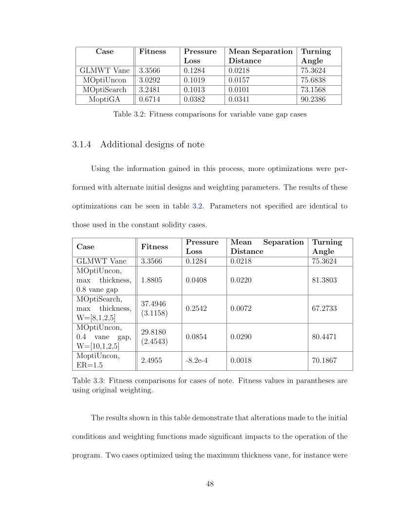
3.1 Fitness comparisons for constant vane gap cases . . . . . . . . . . . . 443.2 Fitness comparisons for variable vane gap cases . . . . . . . . . . . . 483.3 Fitness comparisons for cases of note. Fitness values in parantheses
are using original weighting. . . . . . . . . . . . . . . . . . . . . . . . 483.4 Comparison of MISES and STAR-CCM+ loss values . . . . . . . . . 54
v
List of Figures
1.1 Turning vanes in the Glenn L. Martin Wind Tunnel [1] . . . . . . . . 11.2 Turning vane designs and associated loss values [2] . . . . . . . . . . . 21.3 Blueprints of the GLMWT circuit . . . . . . . . . . . . . . . . . . . . 21.4 Dimensioned sketch illustrating possible test section expansion. . . . . 41.5 Original (solid line) and optimized (dashed line) vanes from Ref. [10] 7
2.1 Example bezier curve displaying control points and generated curve. . 102.2 Illustration of geometric analysis for expansion ratio . . . . . . . . . . 142.3 Vanes used in parameter sweeps . . . . . . . . . . . . . . . . . . . . . 272.4 Tunnel models used in STAR-CCM+. Top left is non-expanding, top
right is expanding, bottom center is detail view of the vanes. . . . . . 292.5 Mesh view of the non-expanding model . . . . . . . . . . . . . . . . . 302.6 Detail views of the mesh at the trailing edge to illustrate prism layers 30
3.1 Parameter sweep plots for camber. Alpha indicates distance alonginterpolation from current GLMWT vane to modified version. . . . . 34
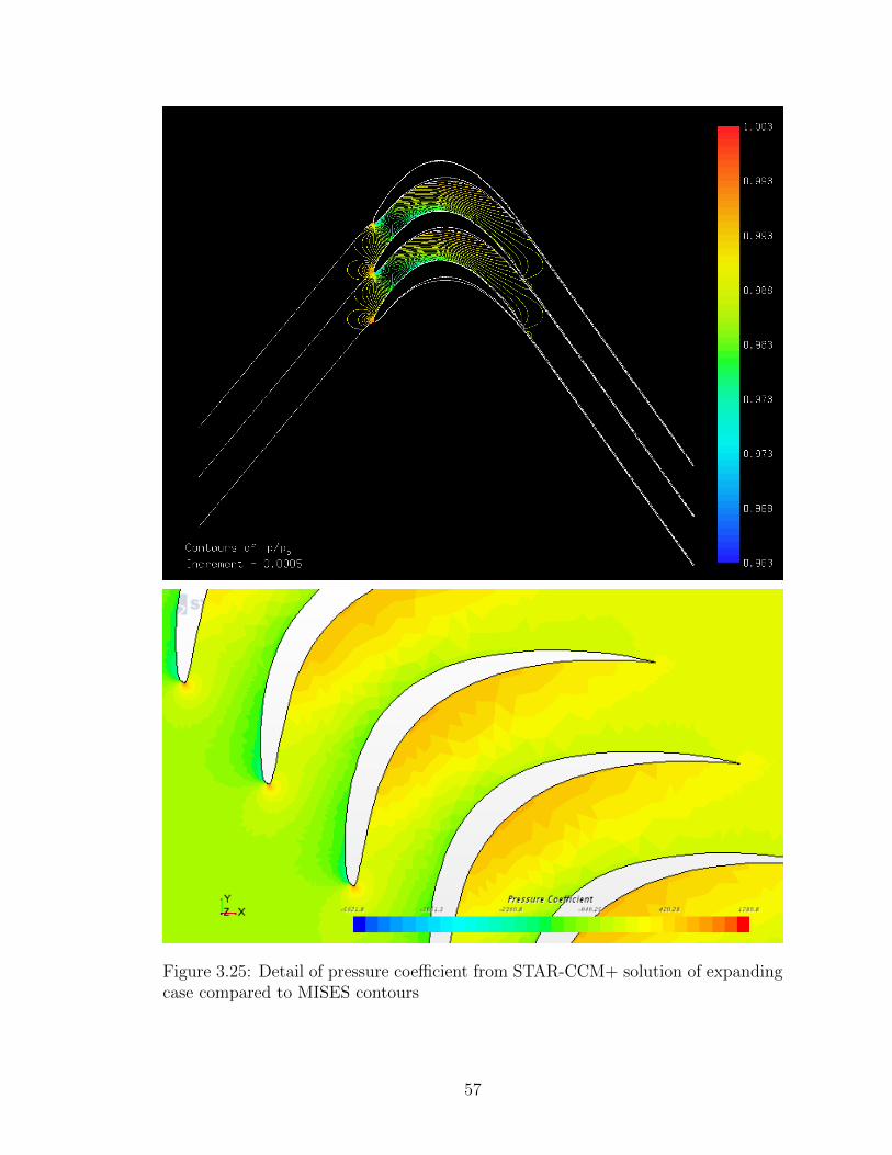
ing case compared to MISES contours . . . . . . . . . . . . . . . . . . 573.26 STAR-CCM+ solution of expanding case using optimized turning vane 583.27 Detail of pressure coefficient from STAR-CCM+ solution of optimized
CAD Computer Aided DesignCFD Computational Fluid DynamicsER Expansion RatioGA Genetic AlgorithmGLMWT Glenn L. Martin Wind TunnelM.I.T. Massachusets Institute of TechnologyNACA National Advisory Committee for AeronauticsPa PascalsLE Leading EdgeSTAR STAR-CCM+TE Trailing Edge
viii
Chapter 1: Introduction
Figure 1.1: Turning vanes in the Glenn L. Martin Wind Tunnel [1]
When designing a wind tunnel for aerodynamic research, there are a near
infinite number of decisions to be made. The choice of returning or non-returning
tunnel is one of the most important of these decisions. Closed return wind tunnels
have lower power requirements than non-returning tunnels as the flow must only be
kept moving by overcoming losses rather than accelerated from stationary. These
benefits, however, come at the cost of significantly increased complexity. Much of
this complexity is related to the need to maintain flow uniformity around corners.
In order to preserve uniform flow and prevent losses in corners, it is necessary to
create turning vanes for each corner. Turning vanes are cascades of airfoils designed
to turn the flow in sections and minimize energy losses. The design of these airfoils
1
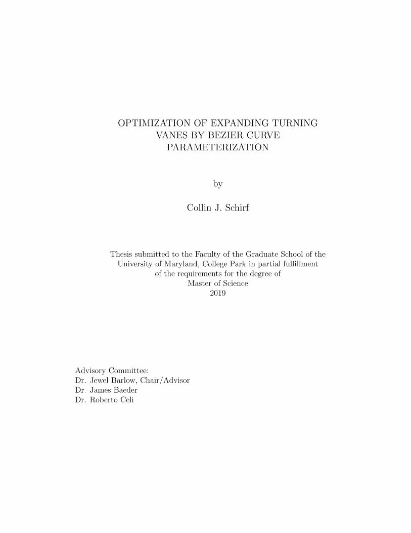
Figure 1.2: Turning vane designs andassociated loss values [2]
can vary from a simple circular arc to a
complex highly cambered airfoil. As with
most aerospace applications, a carefully
considered design can result in improved
performance. The book “Low-Speed Wind
Tunnel Testing” provides data for such an
example where a simple bent plate generates a loss nearly double that of a specially
designed high camber airfoil [2]. For a small amateur tunnel, the larger loss may be
an acceptable alternative to a lengthy design process, but for a dedicated research
tunnel, this loss represents significant increases to operating costs.
Thus, the development of tools for the design of turning vanes is useful to any
who desire to create their own tunnel or improve an existing tunnel. Furthermore,
creating tools which are simple to use could improve the ability of those with less
experience and resources to create effective and efficient closed-return tunnels.
Figure 1.3: Blueprints of the GLMWT circuit
2
1.1 Background and Motivation
The Glenn L. Martin Wind Tunnel (GLMWT) was constructed in 1949 as a
gift to the University of Maryland. The design of the GLMWT was tailored largely
to facilitate aircraft testing [1]. Since its completion, though, the facility has been
used for a variety of applications beyond aircraft. Notably, the GLMWT currently
does extensive automotive testing. To better characterize flows in the wake of these
automobiles and other bluff body type flows, the director of the wind tunnel desired
to extend the test section.
Given that the GLMWT stands on the campus of the University of Maryland,
College Park and is surrounded by other buildings, an extension of the building
to accommodate a longer test section would not be possible. Instead, it was de-
cided that replacing the first corner with an expanding corner could be investigated.
This alteration would allow the first diffuser to be shortened and the test section to
be lengthened without alterations to other portions of the tunnel. Even a modest
expansion ratio would allow significant lengthening of the test section. Basic calcu-
lations using the current diffuser’s area ratios show that an expansion ratio of 1.2
in the corner would allow about 17 feet to be added to the test section . Figure 1.4
demonstrates this alteration graphically.
Unfortunately, the design of turning vanes for use in expanding corners is not
an extensively studied or documented field. For this reason, the research presented
in this thesis was necessary to bridge the gap and assist in the investigation of a
potential redesign.
3
Figure 1.4: Dimensioned sketch illustrating possible test section expansion.
1.2 Prior Work
Though expanding cascades have not been extensively studied, a few papers
have been written on designs for use in non-expanded corners. This research has also
been supplemented by research in separate areas with results applicable to turning
vanes such as the design of turbomachinery and general flow simulation though
Computational Fluid Dynamics (CFD).
1.2.1 Theoretical treatment of flow about airfoil cascades
In 1944, the National Advisory Committee for Aeronautics (NACA) published
research describing the use of potential flow theory to predict the flow about a lattice
of airfoils with the aid of conformal mapping. This method allowed the pressure
distributions about the airfoils to be calculated for incompressible, irrotational flows
4
[3]. Originally intended for application to any infinite cascade of airfoils, this work is
cited in later works dealing with the optimization of vanes for use in turbomachinery
such as the paper “Analysis of Transonic Cascade Flow Using Conformal Mapping
and Relaxation Techniques” from 1977 [4]. A 1947 paper by Spurr extended the
capabilities of this type of analysis with the use of thin airfoil theory. In this
work, a method for calculating the cascade properties of an airfoil are related to
the properties of a lone airfoil [5]. Both the 1944 and 1947 works were primarily
concerned with the pressure distribution along the airfoil in these cascades rather
than the flow properties behind the cascade.
In the 1970’s, the increasing computational power and refinement of compu-
tational methods led to the development of CFD solvers tailored to airfoil cascades.
The development of one such solver is described in the paper “A New Approach in
Cascade Flow Analysis Using the Finite Element Method.” These methods eschewed
the explicit use of conformal mapping for the solution of the potential flow about
airfoil cascades. Instead the author used a finite element method more common
in modern CFD [6]. With this type of solver, a more accurate picture of the flow
properties ahead of and behind turning vane cascades could be generated.
In the late 2000’s, Dr. Mark Drela of M.I.T. developed the MISES flow solver
for use in turbomachinery applications. This flow solver utilizes a Newton method
to solve for the flow about a single airfoil and uses periodic boundary conditions
to extend this flow to an infinite cascade. Included in the solver are tools for grid
generation, flow property specifications, flow visualization, and optimization tools.
This suite has tremendous capabilities and the specialization in infinite cascades
5
allows the options to be tailored to suit the needs of those designing for a number
of applications [7].
1.2.2 General turning vane design
As previously discussed, there is some difficulty in finding research directly
related to turning vane design. Much of this design work was performed as a matter
of necessity based on the aerodynamic research available at the time and was not
documented publicly. Despite this, some design processes can be seen in the pa-
per “Wind Tunnel Turning Vanes of Modern Design” published by NASA in 1986.
In this paper, an inverse technique was used to generate an airfoil to create a de-
sired pressure distribution whose performance was verified with an inviscid CFD
code. Using this process, a modest improvement in corner loss was achieved over a
previously-used arc-shaped vane [8].
More modern design procedures can be found in a paper from the Polytechnic
University of Madrid. This paper is notable as it describes a somewhat simpler opti-
mization process using the tools provided by MISES. To facilitate easy construction,
the shape of the airfoil was assumed to be defined by a quarter circle on the lower
surface and a parabolic arc on the upper surface. Based on this assumption, pa-
rameter sweeps were performed on the maximum thickness and leading edge radius
to find the design with the lowest pressure loss across the corner. Following this,
MISES was used to manually optimize the vanes. Also described in the article is
the use of MATLAB to set up required files quickly and accurately [9].
6
1.2.3 Expanding turning vane design
Figure 1.5: Original (solid line) and optimized (dashed line) vanes from Ref. [10]
The lack of solid information about designing turning vanes for expanding
flows was breached somewhat by a paper from the Royal Institute of Technology in
Sweden. This paper by Bjorn Lindgren and Arne Johansson describes the redesign
of a small-scale subsonic tunnel to include an expanding corner. As a part of this
redesign, the turning vanes in the first corner of this tunnel were optimized for use
in the new corner. The inverse design features of MISES were utilized to alter the
previous vane design to work with a two dimensional expansion ratio of 4/3. The
resulting turning vanes had a pressure-loss coefficient of 0.041 which is only slightly
worse than the original vane [10].
1.2.4 Bezier curve parameterization
While there are many ways to define an airfoil, for the sake of optimization it
is beneficial to find a method which reduces the number of design variables required
to fully define the shape. Bezier curves present one such method which has been
described in a number of papers. The paper “A Survey of Shape Parameterization
7
Techniques”, for instance, describes the use of Bezier control points in airfoil opti-
mization as a way to reduce the number of design variables while still covering a
large amount of design space. The paper also notes the benefits of this method over
similar spline techniques due to the fairly close relation between the control points
and the position of the defined curves [11].
The usefulness and versatility of this form of parameterization are expanded
upon by “Optimum aerofoil parameterization for aerodynamic design”. This pa-
per demonstrated the ability of various configurations of multiple low order Bezier
curves with positions calculated by airfoil parameters to replicate existing NACA
airfoils. Though there was some discrepancy for all configurations, the close match-
ing indicated a good ability to represent a wide array of geometries with few control
points [12].
1.3 Scope of Present Research
The research discussed in this thesis will focus primarily on the development of
a tool for use in the process of optimizing turning vanes for expanding corners. For
this reason, simplifying assumptions will be made and the vane designs presented
will not be claimed to be the ideal vanes for use in the GLMWT. For instance,
the expansion will be assumed to occur only in the two-dimensional plane. This
ignores some features of the GLMWT, but is sufficient to demonstrate the efficacy
of the design process and simplifies the analysis to work with the primarily two
dimensional solver used by MISES. Possible amendments to this process which may
8
overcome this limitation will be discussed in the further work section.
In addition, due to time and resource constraints, results will be verified only
by comparing to the MISES model of the current vane design to a more robust
commercial CFD code. Though this will not entirely guarantee the accuracy of the
results gained with MISES, agreement between the two solvers should give some
proof that optimizations made using this design tool will reflect improvements in
real flows.
1.4 Contributions of Present Research
This work will generate a tool with which flow conditions incident at a corner
may be used to optimize a design for turning vanes to use in that corner. The
aim of this work is to simplify the optimization process by eliminating the need for
inverse designs and intimate knowledge of MISES so that less experienced designers
can achieve reasonable designs. The research additionally aims to allow optimized
designs to be less reliant on the initial design.
9
Chapter 2: Methodology
2.1 Airfoil Definition
The geometry for each airfoil design was defined using Bezier curves. The
usage of Bezier curves to define the airfoil provides three distinct advantages. First,
the relatively small number of control points used to describe the airfoil drastically
reduce the number of design variables in optimization problems and thus reduces
computational cost. This is especially pertinent to derivative based optimizers since
finite differencing requires at least one additional function evaluation per design
variable for each iteration.
Figure 2.1: Example bezier curve displaying control points and generated curve.
10
Second, the nature of these curves allows large changes over the entire length
of a curve to be made with the movement of a single control point. This gross
alteration helps to prevent some of the strange design features that can arise in
airfoil optimization.
Finally, the use of multiple Bezier curves allows fine optimization to be per-
formed in a number of different ways by pinning or relating certain control points.
Pinning the endpoints of a curve near the leading edge, for instance could allow
the leading edge curve to be more finely tuned by increasing the density of control
points in the area. This is of particular import in the design of turning vanes where
the leading edge can define the sensitivity to incoming flow alterations [2].
2.1.1 Bezier curve definition
As discussed previously, Bezier curves are a parameterization method for defin-
ing curved lines through the use of a small number of control points. The distance
from these control points is then interpolated to generate the necessary curves.
Mathematically, this interpolation can be described for a curve of (N − 1)th order
using the equation:
X(t) =
(N
1
)Cx1(1 − t)N +
(N
2
)Cx2(1 − t)N−1t+ ...
(N
N
)CxN ; 0 ≤ t ≤ 1 (2.1)
An equation of the same form may be used to describe an arbitrary number of addi-
tional coordinates in other dimensions, though for this research only two dimensions
will be used.
11
Helpfully, this operation may be converted to a matrix form by expanding the
polynomial terms. For N = 2, this formula becomes:
X(t) = ( 1 t t2 )
1 0 0
−1 2 0
1 −2 1
Cx1
Cx2
Cx3
(2.2)
The matrix needed to perform this operation can be defined by populating the
main diagonal with the correct row of Pascal’s triangle for the number of control
points then populating each Kth diagonal with the Kth value of the correct row
multiplied by the Kth row of the triangle and −1K . For clarity, a sample execution
of this procedure is shown in table 2.1.
11 1
1 2 11 3 3 1
First four rows of Pascal’striangle, final row repre-sents main diagonal.
1 ∗ [1 3 3 1]−3 ∗ [1 2 1]
3 ∗ [1 1]−1 ∗ [1]
Definition of each diagonalstarting with main diagonaland heading toward the cor-ner.
1 0 0 0−3 3 0 03 −6 3 0−1 3 −3 1
Final matrix.
Table 2.1: Demonstration of Bernstein matrix creation
More information on Bezier curves is available from Ref. [14].
12
2.1.2 Smoothness constraints
Another useful mathematical feature of Bezier curves is that the curve becomes
tangent to the slope between the endpoint and previous control point at the endpoint
of the curve. This makes enforcing smoothness between two curves simple. Noting
that the endpoint for one curve will be the first control point of the next, this
relationship may be written:
y2 − y1x2 − x1
=y3 − y2x3 − y2
(2.3)
Assumng that the point x3 will be altered, a value for y3 enforcing smoothness
can be found:
y3 = y2 +(x3 − x2)(y2 − y1)
x2 − x1(2.4)
Using these types of constraints, it is possible to generate smooth airfoils with
multiple curves of smaller orders. In practice, this was necessary because the matrix
needed to generate a curve with more than 35 control points creates large truncation
errors and does not generate the desired airfoil.
2.1.3 Additional constraints
For these optimizations, the airfoils were defined by four Bezier curves of
fifth order. The endpoints of each curve were shared to ensure continuity, and
the smoothness constraint discussed in the previous section was used to ensure
13
smoothness. In theory, it would be possible to generate an infinitely sharp leading
edge at a specified point by omitting this constraint, but due to the ability of a
blunt leading edge to mitigate sensitivity to variance in the incident flow conditions
this configuration was not investigated [2].
Additional constraints were placed to ensure that the vane was feasible. Most
important of these was the constraint on self-intersection. A MATLAB program
written by Antoni Canos was used to check each airfoil curve for self-intersection
[15]. Whenever a vane with intersecting upper and lower surfaces is created, an error
is thrown. Using try and catch functions allows this error to act as a sort of penalty
function by assigning a poor fitness value to any such cases. A similar process was
used to prevent situations where the upper surface of one vane would intersect the
lower surface of the next vane due to high thickness, high camber, or low vane gap
distance.
2.1.4 Expansion ratio representation
Figure 2.2: Illustration of geometricanalysis for expansion ratio
Once the airfoil has been defined, it
is necessary to have a parameter denoting
the expansion ratio being applied to the
cascade. The geometric analysis shown in
figure 2.2 demonstrates that the inlet and
outlet angles are sufficient to describe the
expansion ratio. This geometric analysis
14
takes the centerline of the cascade as the straight line between the inner and outer
corner of the wind tunnel walls and uses the expansion ratio to set a relation between
the width of the tunnel at the inlet of the turn and the width at the outlet. Using
trigonometric functions to solve for the flow angle incident on the turning vanes
gives the following definition:
β1 =π
2− β2 (2.5)
A2 =A1
sin(π2− β1)
(2.6)
A2 =A3
sin(π2− β2)
(2.7)
A1
sin(π2− β1)
=A3
sin(β1)(2.8)
A3
A1
= ER (2.9)
A3
A1
=sin(β1)
cos(β1)(2.10)
ER = tan(β1) (2.11)
This definition is expedient given that MISES defines its inlet angle in the same
tangent form. Thus, the specification of the expansion ratio can be accomplished
within the standard setup of the program.
15
2.1.5 Solidity definition
Solidity is an important parameter in any study of airfoil cascades as it defines
how close the airfoils are to one another, thus affecting their impact on one another.
This parameter has a number of definitions depending on the aerodynamic context,
but in general, a high solidity indicates a small distance between airfoils and a low
solidity indicates a large distance. For the purposes of this study, the solidity of the
cascades investigated will be defined by the vane gap. This is taken as the vertical
distance between one vane and the next.
2.2 MISES Operation
Analysis with the MISES software occurs in four steps, the first of which steps
is file setup. In order to run, MISES requires a file defining the airfoil geometry
and a file defining the flow constraints and initial values. These files are defined as
blade.xxx and ises.xxx where xxx is an arbitrary case name.
The second step is grid generation, which occurs within the subprogram ISET.
In a traditional case, ISET is used to define grid parameters and inspect the gener-
ated grid before writing to a file. Calling ISET loads the blade.xxx file and uses a
panel code to initialize stagnation streamlines which help to define the boundaries of
the grid. From here, user inputs initialize a grid between these boundaries and alter
any parameters that affect point distribution along the airfoil. Fortunately, much
of this process may be streamlined using a gridpar.xxx file containing parameter
values. Within the context of this optimizer, the ideal value of these grid parame-
16
ters should stay relatively constant, and the operation of ISET can be streamlined
in this manner. Elliptical grid smoothing is also provided to increase the quality of
the mesh. The generated grid with an initial condition defined by the panel code is
output to a file idat.xxx.
Variable Number Definition1 Inlet flow slope2 Exit flow slope5 LE stagnation point6 Grid exit static pressure15 Inlet Mach number
Constraint Number Definition1 Drive inlet slope to SINLin3 Set LE Kutta condition4 Set TE Kutta condition6 Drive inlet POa to 1
γ
15 Drive inlet mach to MINLin
Table 2.2: ISES variables and constraints for program operation
Following the creation of the grid, the subprogram ISES must be called to
complete the third step of the flow solution. ISES iterates the solution to satisfy the
user-specified constraints by altering the user-specified variables. The constraints
used for this paper may be seen in table 2.2. These constraints allow for the pressure
ratio behind the cascade to be found for a given set of upstream flow parameters.
The solver runs the first iteration as an inviscid case before including viscous effects.
This efficiency measure and the use of a Newton flow solver result in convergence
after relatively few iterations, usually less than 15 for the cases investigated. This
step may also be performed by the subprogram POLAR. This program is generally
used to sweep through flow parameters to investigate the operation of a cascade
beyond its design point. Use of this program was determined to be necessary for
17
the procurement of a value for total pressure loss.
The final step of the flow solution is performed by running the subprogram
IPLOT. In standard operation, this program is used to generate and format plots
of flow quantities. While this was used for debugging and testing, the primary use
of IPLOT within this thesis was the creation of field.xxx files. These files contain
data for a number of flow quantities along each streamline. This file simplified the
transfer of data from the idat.xxx file into MATLAB.
These operations are run from the command line and primarily operate through
user inputs to menu prompts. This makes the software difficult to use from within
MATLAB as the command line interactions allowed by the system() function do not
permit the software to input information during program operation. Additionally,
the complexity of the software largely precludes the creation of a MEX file which
would allow operation entirely from within MATLAB. Instead, the packages TCL
and Expect are used to automate the usage of MISES. These packages streamline
the piping process commonly used in batch files to simulate user input. Due to the
similarity of the cases presented during optimization, a single Expect file may be
used to run through each step of the MISES simulation with a single command from
MATLAB. For this research, a file MISExpect was written which sets up the grid,
iterates using POLAR, then outputs the data to a field.xxx file.
Samples of each of these file types can be found in the Appendix to this report,
and further information on MISES is available from Ref. [7].
18
2.3 Optimization Functions
The field of optimization is quite broad and contains a number of techniques
and methods. To find the best method for optimizing this particular problem,
a number of methods were explored. For the purposes of this investigation, un-
constrained optimization was deemed to be the most useful. This is due to the
fact that mathematically determining the existence of non-feasible designs, such as
those where the turning vane surfaces intersect themselves, would be unnecessar-
ily complex. Instead, a penalty function was added to unconstrained optimization
techniques to discourage non-feasible designs.
The fitness function used in this optimization was a weighted sum of three
parameters. These parameters are the total pressure loss, separation magnitude,
and the difference between the turning angle and a right angle. These parameters
were selected as the pressure loss and lack of separation are the primary needs of
turning vanes. The turning angle parameter is included as a turning angle too high
or too low would likely cause difficulties as the flow propagated through the rest of
the straight tunnel section behind the corner.
2.4 MATLAB Operation
As discussed in prior sections, a number of MATLAB functions were generated
to assist in the optimization presented. Though not all functions were ultimately
used, they will all be presented for the purposes of future work.
19
2.4.1 Bezier curve functions
Two functions were used to define the curves for use in the turning vanes. The
first of these functions was BernMat(). This function automatically generated the
necessary matrix for the calculation of a Bezier curve of order n− 1. This function
was called by a separate function Bez(). Bez() takes two vectors of control points,
the number of points to be plotted in the curve, a string signifying whether multiple
curves are to be used, and an optional vector containing the order of each curve.
Using these inputs, the program uses for loops to generate the specified curves and
outputs a vector of x values and a vector of y values.
2.4.2 File setup functions
As most MISES operations require the file they reference to be generated
before the program will operate, creating functions that allow automatic creation of
these files was one of the most important steps of this research.
The first of these functions is V aneBuild(). This function takes the control
points, normalized vane gap distance, and an input structure containing flow data
specified by the user. The function calls Bez() with the given inputs and writes the
results to a file blade.xxx. The file name and additional parameters are taken from
the input structure.
The second of these functions is InputSetup(). This function creates the file
ises.xxx for a given file name using both data specified in an input structure and
values coded into the function. Though hard-coding values is a less than ideal
20
manner of specifying them, the values handled in this way were determined to be
unlikely to change for any case handled by the program. If necessary, these values
could be added to the input structure and the function altered to accommodate the
new format.
DataRead() reads the field.xxx file for a specified file name and outputs an
average pressure loss, mean separation distance, and outlet flow angle. A similar
file DataReadFit() performs the same process, but uses user-specified weights to
calculate a fitness value from these three values. These files also call SepV al() which
reads the field.xxx and blade.xxx files to compare the locations of the blade surfaces
and stagnation streamlines. These distances are averaged over the vane to create an
approximate measure of the magnitude of separation present on the given airfoil.
2.4.3 Program operation functions
Of equal import to the functions which set up the files are the functions which
operate the MISES program. The most vital of these is MISESEval which uses the
system() function to run the Expect file MISExpect from the command line. If the
command is not carried out, an error is thrown.
To simplify other codes, the file MISES() was written. This file takes the
same inputs as V aneBuild() and runs V aneBuild(), InputSetup(), MISESEval(),
and DataRead(). As with DataRead(), a similar program MISESFit() is used to
output a fitness value directly rather than the three values output by DataRead().
21
2.4.4 Optimization functions
With the ability to run and gather results from MISES handled by the func-
tions described previously, functions for optimizing vanes within this environment
were simple to create. Similar to Lindgren and Johansson [10], the normalized drop
in total pressure across the vane was the main value being queried by the optimizer.
MISES outputs this value with the definition:
ω =piseno2 − po2po1 − p1
(2.12)
This definition, output by the POLAR function, compares the isentropic total
pressure to the mean total pressure and normalizes by the inlet conditions. This
provides a convenient value to minimize to ensure good vane operation. Addition-
ally, this value should be relatively simple to obtain from the StarCCM+ models.
During early testing of some of the optimization functions, it was found that the
method of calculating loss being used at the time only considered flow between the
stagnation streamlines. This allowed large separations to form as the losses due
to these separations were not impacting the fitness values. To counteract this, the
mean separation value was added to the fitness function and highly prioritized by
the weighting. Though the loss calculation was later altered to the one specified
above, this parameter remains useful to ensure as little separation occurs as pos-
sible. Additionally, adding minimal deviation from a specified turning angle as an
additional optimization goal could help to prevent designs which drastically over-
22
turned or under-turned the flow. With these goals and parameters set, the functions
could be created and tweaked.
The first of these functions is MOptiUncon. This function performs a Broyden-
Fletcher-Goldfarb-Shanno (BFGS) optimization aimed at minimizing the fitness
function calculated by MISESFit. This function takes an initial design configuration
and a few run parameters such as tolerance and finite differencing calculation step
size and outputs a new design and the final design’s fitness value. The smoothness
constraint discussed in section 2.1.2 was applied within this function as it effectively
reduces the number of design variables and the smooth transitions were deemed to
result in a better quality of vane.
Two more functions were created to perform the same task with different opti-
mization functions. One, MOptiSearch.m, used fminsearch() to optimize the turning
vane while the other, MOptiGA.m, used ga(). The fminsearch() function uses a form
of simplex algorithm to optimize a given function. Conversely, ga() operates a ge-
netic algorithm to optimize the problem. Due to the nature of the penalty function,
it is necessary to provide all three functions with a feasible initial design to achieve
a feasible result. In testing, non-feasible designs were unable to provide a reasonable
direction for the optimizers within the design space that pushed the altered designs
to become feasible. MOptiGA was particularly susceptible to this difficulty as stan-
dard operation allows the function to generate the initial population without regard
to feasibility. As such, an expression to generate the initial population by adding
bounded random values to each of the parameters was added to this function.
23
2.4.5 Miscellaneous functions
In addition to the functions described above, a few functions were written
for convenience or written and subsequently determined to be unnecessary. The
function InStructSet(), for instance, is a function that automatically creates the
necessary input structure for the file setup and MISES operation functions from a
set of hard-coded values. This function is useful to ensure that element names within
the structure are consistent with those used in the functions as well as to quickly
generate many structures with similar values to accommodate slightly varied cases.
The functions V aneCalc() and V aneF it() were used early in testing to find
values of the Bezier Parameters similar to those of the current turning vane. These
functions used fminsearch() and a distance calculation to optimize the parameters
such that the curve generated by Bez() passed through a given set of points along
the current GLMWT turning vane design. The generation of these parameters
was useful for creating an initial, feasible design for later optimizations as well as
providing good practice with the MATLAB optimization toolbox.
The function GridPar() was written to automatically generate a gridpar.xxx
file for use in ISET operation. It was quickly determined that adding a pause
function to the optimization programs and allowing a manual setup of the first
parameter set was more advantageous, and this program was not utilized.
24
2.5 Flow Similarity Parameters
To ensure the applicability of the flows found using MISES to those generated
in the real world, it was necessary to match flow parameters. For this flow, chord
Reynold’s matching and Mach number matching were used to achieve this. Using
standard sea level conditions taken from Ref. [16] for viscosity and density, the flow
speed and characteristic length were calculated by using the flow speed at the first
corner corresponding to the tunnel’s top speed and the chord length of the original
vane. Likewise, the flow speed at the first corner was used to calculate the Mach
number. Noting that the desired setup of the expansion ratio would result in a
decreased area at the corner, a relation between both similarity parameters and the
expansion ratio was generated. This process, largely predicated on the continuity
equation, can be seen below where the subscript c denotes a value at the corner
entrance, ts denotes a value at the test section, and the notation A′c denotes the
original area at the corner:
Re =ρvcl
µ(2.13)
vc = vtsAtsAc
(2.14)
Ac = A′c · ER (2.15)
AtsAc
= 0.3269 · ER (2.16)
Re =1.204kg/m3(103m/s(0.3269 · ER))(0.6515m)
1.789 · 10−5Pa · s(2.17)
25
Re = 1.476 · 106 · ER (2.18)
A similar process can be used for Mach number:
M =vca
(2.19)
a = 343m/s (2.20)
M = 0.0982 · ER (2.21)
Additionally, for simplicity, all design dimensions were scaled by the chord
length of the current GLMWT turning vane.
2.6 Data Acquisition
Once the functions were created, data for this research was gathered in a
few steps. The first of these steps was a simple parameter sweep similar to the one
performed by Lopez et al. in Ref. [9]. This process served a few purposes. First, the
sweep demonstrated the ability to operate MISES from within MATLAB on valid
vane geometries. Second, the results of the sweep gave some understanding of the
effects of these parameters on the pressure loss associated with these blunt turning
vanes. To this end, camber, thickness, and cascade solidity were all investigated for
a simply modified version of the current GLMWT first corner vane. The vanes can
be seen in figure 2.3. Finally, the sweep helps to bridge some gaps left by Lopez et
al.[9] in terms of camber and cascade solidity.
26
Figure 2.3: Vanes used in parameter sweeps
Following the parameter sweep, a number of optimization cases were per-
formed. First, each optimizer was run using the GLMWT vane as an initial con-
dition and constraining the vane gap to a constant value. This process used an
expansion ratio of 1.2, but cases with other expansion ratios were also performed to
test the functions. Second, the same optimization was performed using a variable
solidity to determine if the added design parameter would alter the vane design
significantly. During this process, alterations and fixes to each of the solvers were
made to ensure acceptable performance.
Finally, the lessons from the parameter sweep and the many optimization cases
were taken and used to experiment with new starting points and parameters. These
cases spanned a wide range of investigations and had a large number of outcomes,
so a select few with notable outputs were included in this report.
27
2.7 Verification
The results of this optimization were verified using the CFD software STAR-
CCM+. The vane design for both the current GLMWT first corner design and the
newly optimized design were modeled in the CAD package SolidWorks and imported
into STAR.
2.7.1 Model generation
The models for verification were generated using the tools provided in Solid-
works. First, the blade.xxx file is imported into Excel and the Cartesian coordinates
of the vane are prepared for import into SolidWorks. This preparation involves scal-
ing by the original vane chord to ensure flow similarity and placing the data in
the correct format. Next, the vane is loaded into SolidWorks and used to create
a 2-D curve. This curve is copied using the pattern tool to generate the correct
number of vanes for the present case with the correct cascade angle to generate the
necessary expansion ratio. Straight and parallel tunnel walls are then created to
allow for proper wake propagation. These walls were made to be roughly 5 chord
lengths ahead of the corner and 10 chord lengths behind the corner. Finally, a semi-
arbitrary curve was generated at the tunnel wall using a four point style spline. This
spline was constrained to be tangent to the inlet and outlet walls and dimensioned
to appear similar to the vane shape. Given that MISES has no way of handling wall
geometries, the primary point of interest in this verification will be away from the
wall and wall geometry is thus less influential. Figure 2.4 shows the models used.
28
Figure 2.4: Tunnel models used in STAR-CCM+. Top left is non-expanding, topright is expanding, bottom center is detail view of the vanes.
2.7.2 Meshing
To ensure proper handling of boundary layers, the mesh generated within
STAR-CCM+ was generated such that the maximum wall y+ was between 1 and
5 to fit within the bounds of the wall functions used. To achieve this, prism layers
with a controlled thickness at the wall and defined total thickness were added. For
simplicity, a triangular mesh was used in all other regions with wake refinement
controls added to the vane geometry. The mesh for the non-expanding case using
the GLMWT vane can be seen in figure 2.5 with detail views in figure 2.6. Major
meshing parameters can be seen in table 2.3.
29
Variable Number DefinitionParameter ValueMinimum Surface Size 1.0e-4Number of Prism Layers 15Prism Layer Near Wall Thickness 1.0e-5Prism Layer Total Thickness 0.01mVane Surface ControlsTarget Surface Size 0.05mIsotropic Wake Size 0.05mWake Growth Rate 1.25
Table 2.3: Non-default meshing parameters
Figure 2.5: Mesh view of the non-expanding model
Figure 2.6: Detail views of the mesh at the trailing edge to illustrate prism layers
30
2.7.3 Simulation setup
To properly model the conditions in the tunnel, the similarity parameters used
in the MISES file are related to the conditions of the tunnel modelled in STAR-
CCM+. To do this, it was necessary to alter the properties of air in the simulation
to have the same dynamic viscosity as the one used to calculate the Reynold’s
number in the simulation. By setting the inlet velocity to match the specified inlet
Mach number and ensuring static temperature and the chord length of the model
were correct, the correct Reynold’s number was achieved naturally.
In selecting the models, the problem was assumed to be steady and the air
was assumed to act as an ideal gas. Turbulence was modelled with a Realizable
K-Epsilon solver. All other models were selected as the STAR defaults for a two
dimensional steady problem.
2.7.4 Data collection
To assess the similarity in solutions between MISES and STAR, three monitors
were considered. First, a visual assessment of pressure and velocity contours was
used to verify that no apparent errors had occurred within the simulation. Second,
the pressure contours around the vane were examined and compared to the plot
generated for the identical case using MISES. Last, a line probe was generated
parallel to the cascade about one chord length away and not reaching the walls.
This probe was used to calculate the mean pressure loss and to compare with these
values from MISES.
31
Chapter 3: Results
3.1 MISES Results
On operating the MATLAB wrapper for MISES, there are a number of ob-
servations to be made. First, the speed of operation should be noted. As expected
from the typically quick convergence and relatively low computational requirements
of MISES, operation was relatively quick. For reference, the parameter sweep rou-
tine generates and solves 60 MISES cases and takes roughly ten minutes to complete
on a personal desktop with a 6-core i7 processor and 16 GB of RAM. Unfortunately,
the nature of optimizers prevents the same from being true for full optimization
cases. Dependent on the method used and tolerances specified, the optimizers took
between thirty minutes and multiple hours to output a converged value. Compared
to an optimizer using a different CFD solver, this is fairly quick. Additionally, the
quick convergence of each case indicates that methods with better convergence could
speed this total process in future iterations.
Second, the need for good engineering judgment in the operation of these
programs must be noted. Though the optimization process requires less knowl-
edge of the aerodynamics than an optimization within MISES, the ability of im-
proper weighting specifications, initial vane definitions, and other issues to cause
32
non-convergence or to generate vanes with poor performance indicates a need for
careful consideration of these parameters. Further, a basic understanding of MISES
operation and aerodynamics is needed to verify the results of any optimization.
Certain functions generated designs with non-viable streamlines or which did not
converge and had questionable pressure profiles warranting additional scrutiny.
3.1.1 Parameter sweep
The results of the parameter sweep confirmed some theories about the effects
of the parameters while also contributing some new insights. It should be noted that
a larger value for loss represents a worse vane as does a larger value for separation.
Additionally, the turning angle is defined as the angle of the outer corner of the wind
tunnel. As such, smaller values represent sharper turns and a value of 90 degrees
represents a perfectly right-angled turn. Values below 90 degrees will be referred to
as over-turning and values above as under-turning.
Sweeping from the current vane to a modified, high-camber version showed
that increasing this camber generated increased pressure losses and increased over-
turning. This is generally not surprising as the higher camber will result in an
effectively larger angle on the latter portion of the vane and flow tangency will
encourage a larger turning angle due to this. Despite the larger losses, the higher
turning angle could prove beneficial in cascades with a larger vane gap. Depending
on what flow features are generating the largest pressure losses, having fewer vanes
spaced further apart with a higher turning angle could help to turn the flow with
33
Figure 3.1: Parameter sweep plots for camber. Alpha indicates distance alonginterpolation from current GLMWT vane to modified version.
less overall pressure loss. Also notable is the gradual increase in mean separation
distance. This seems to stem from the fact that the larger camber induced a larger
Figure 3.2: MISES plot of maximum cambervane solution
adverse pressure gradient along the
leading edge of the lower surface and
trailing edge of the upper surface
which caused a larger separation to
form. This can be demonstrated in
figure 3.2 which shows the stagnation
streamlines generated by MISES for
the maximum camber vane.
34
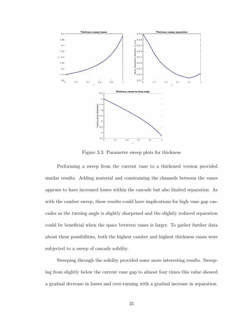
Figure 3.3: Parameter sweep plots for thickness
Performing a sweep from the current vane to a thickened version provided
similar results. Adding material and constraining the channels between the vanes
appears to have increased losses within the cascade but also limited separation. As
with the camber sweep, these results could have implications for high vane gap cas-
cades as the turning angle is slightly sharpened and the slightly reduced separation
could be beneficial when the space between vanes is larger. To gather further data
about these possibilities, both the highest camber and highest thickness vanes were
subjected to a sweep of cascade solidity.
Sweeping through the solidity provided some more interesting results. Sweep-
ing from slightly below the current vane gap to almost four times this value showed
a gradual decrease in losses and over-turning with a gradual increase in separation.
35
Figure 3.4: Parameter sweep plots for solidity
It seems that a vane gap that is too high induces larger separation as the larger
distance between vanes limits the propagation of the flow information imparted by
the vanes. Thus, a large vane gap limits the ability of the upper surface of one
Figure 3.5: MISES plot of 0.7 vane gap solution
vane to prevent separation on the
lower surface of the next vane by
imposing a flow direction and vice
versa. This effect can be seen
in the stagnation streamline shape
of figure 3.5. It is unclear what
causes the convergence failure at
0.9, but the most likely culprit is
36
instability in the separation causing an unsteady problem that MISES cannot con-
verge.
Figure 3.6: Solidity sweep for max camber vane
Repeating the solidity sweep with the high camber and high thickness vanes
shows similar results, but demonstrates the effects of the altered designs. Overall,
as the distance between the vanes increased, the losses incurred decreased, but the
separation caused increased. Many of the solidity values for camber did not converge,
likely for similar reasons to the non-convergence in the camber sweep. Due to this
lack of data, it is unclear what effect the solidity had on the high camber vane, but
the general trend and inability to solve the problem indicates that high camber,
intermediate vane gap designs are not the best to pursue. The maximum thickness
vane presents an enticing case around a normalized vane gap of 0.8 where the loss
37
Figure 3.7: MISES plot of maximum thick-ness vane at 0.8 vane gap
is lower than that of the standard
vane at a low vane gap and the turn-
ing is near 90, though the mean sep-
aration distance is higher. This case
can be seen in figure 3.7. As specu-
lated in the discussion of the thick-
ness sweep, the added material limits
the size of the separation. Based on the contours shown, an adjustment to fur-
ther thicken the vane and alter the angle of the trailing edge could overcome this
separation even at a high vane gap.
Figure 3.8: Solidity sweep for max thickness vane
38
Figure 3.9: Expansion ratio sweep
Finally, sweeping through a number of expansion ratios demonstrates some
unexpected phenomena. The decrease in both losses and separation seem to run
counter to what one could expect from increasing the expansion ratio for a vane
not optimized to that expansion. It is possible that this is the result of effectively
pitching the airfoil because of the definition of expansion ratio in the parameters.
Running two cases at ER=1.3 and ER=1.5 returns the plots in figure 3.10. These
plots are very similar, but the differences in the parameters may help to explain some
of the strange results seen in the sweep. The difference in inlet pressure ratio, for
instance, could be altering the loss calculation as the formula used may be converted
to the form seen in equation 3.1 by presuming that po1 = piseno2 .
39
ω = (1
1 − p1po1
)(1 − po2po1
) (3.1)
Because the ratio in the denominator decreases as expansion ratio increases, it
is possible that the actual loss in static pressure was greater for the larger expansion
case but inflated by the normalization for the other cases.
Figure 3.10: Comparison of ER=1.2 and ER=1.5 case MISES solutions
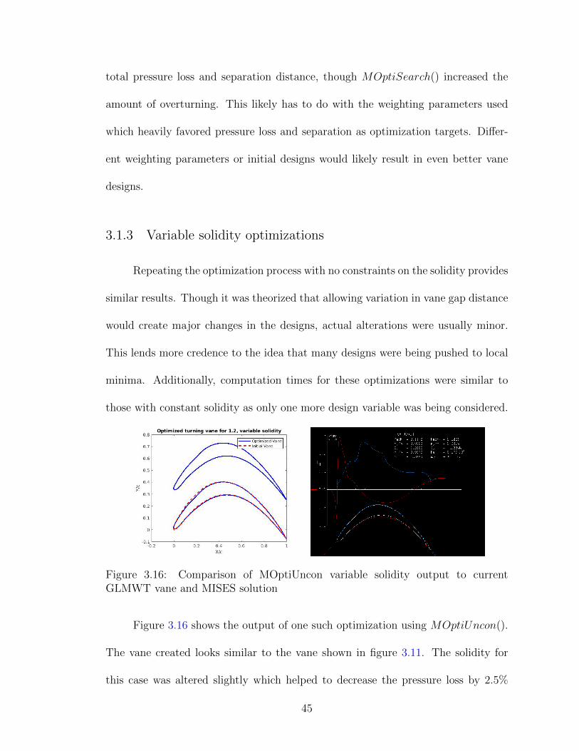
3.1.2 Constant solidity optimizations
Setting up the optimization functions was a difficult process, but ultimately
resulted in some decent optimization tools. The main difficulties in setting up these
functions were determining what file formats and function syntaxes would work with
the prebuilt optimization functions. Once this process was complete, finding proper
option values and fitness function weights took more experimentation. Despite this,
the speed of operation made experimentation less odious. The following vanes were
generated using the weighting vector [10, 5, 0.1, 0.4].
40
Figure 3.11: Comparison of MOptiUncon constant solidity output to currentGLMWT vane and MISES solution
Understandably, MOptiUncon() was the fastest of the optimizers. With rea-
sonably high tolerances, a single optimization case usually took around an hour to
complete. Additionally, the optimizations were generally pushed towards cases with
quick convergences indicating little to no separation or major viscous effects. One
such case can be seen in figure 3.11. This optimization was run with an expansion
ratio of 1.2 using the original turning vane as the initial design. The results in this
case illustrate some of the features common in MOptiUncon() cases. The slight
indent on the upper surface near the leading edge, for instance, is a feature that
appeared in many cases. This feature appears to counteract some of the adverse
pressure gradients that can appear and create separation. As such, very little sepa-
ration appears in this design. It must be noted that in the process of testing these
functions, the MOptiUncon() function had a tendency to fail to alter the design
if not given the correct tolerance parameters. Troubleshooting this optimizer was
also more difficult than the others due to the lack of visualization tools provided
to observe the current state of any optimization case. Additionally, final designs
were very similar to the initial designs, showing that the optimizer had difficulties
41
moving away from local minima.
Figure 3.12: Comparison of MOptiSearch constant solidity output to currentGLMWT vane and MISES solution
MOptiSearch() took longer to converge. With a similar tolerance, this opti-
mizer took roughly one to three hours to complete. A characteristic design generated
with this function can be seen in figure 3.12. This design illustrates the tendency
of this optimizer to grossly alter the trailing edge as well as the mid-airfoil fea-
tures. The features demonstrated in this design are also much different than those
gained with MOptiUncon(). The strange indent seems to interact with the pressure
gradients to help minimize separation on the lower surface. Plotting a contour of
Figure 3.13: Total pressure loss contours for optimized
vane. Blue areas indicate larger total pressure loss.
total pressure losses as
in figure 3.13 illustrates
the possible benefit of
this method as the most
prevalent losses were those
experienced at the lower
surface separation bound-
ary. An unfortunate fea-
42
ture of this optimizer is its tendency to query a large number of infeasible designs.
Because ISES is being run from within POLAR, it is not possible to directly con-
strain the allowed number of iterations. This combination is largely responsible for
the lengthy optimization. This length was helped by the in-built visualization as it
was more apparent when cases were not running correctly. If all initial values were
the penalty function value, for example, it was immediately clear that an error was
occuring and the optimization should be stopped.
Figure 3.14: Function value monitor from MOptiSearch
Figure 3.15: Comparison of MOptiGA constant solidity output to current GLMWTvane and MISES solution
43
As with most genetic algorithms, MOptiGA() took a long time to run. This
optimizer could take close to eight hours to complete a single case. Though it
sometimes reaches a value much sooner, these values were often due to the initial
population all being of poor fitness or luck to find a particularly good design early.
Regardless, this long convergence time may be worthwhile as genetic algorithms
help to avoid local minima. The relative similarity between the starting and ending
profiles of the other two optimizers indicate that there are numerous local minima to
be found and the overall design could suffer by using these solvers without accounting
for this fact. The output of a MOptiGA() case can be seen in figure 3.15. Though
this case was relatively similar in shape to the original design, the slightly extended
chord length was a feature not seen in any of the other optimizers. The chord length
was not constrained in any way, but it is likely that the many control points defining
each curve diminished the effects of any one point moving to alter this parameter.
The results of a single optimization case beginning from the GLMWT vane for
each solver can be seen in table 3.1. This table illustrates some of the differences in
[1] “Glenn L. Martin Wind Tunnel” Available: https://windtunnel.umd.edu [re-trieved 22 Feb. 2019].
[2] Barlow, J. B., Rae, W. H., Jr., and Pope, A., “Wind Tunnel Design,” LowSpeed Wind Tunnel Testing, 3rd ed., Wiley, New York, 1999, pp. 61-135.
[3] Garrick, I. E., “On the Plane Potential Flow Past a Lattice of Arbitrary Air-foils,” NACA TR-788, January 1944.
[4] Ives, D. C., and Liutermoza, J. F., “Analysis of Transonic Cascade Flow UsingConformal Mapping and Relaxation Techniques,” AIAA Journal, Vol. 15, No.5, 1977, pp. 647-652.
[5] Spurr, R.A., and Allen, H. J., “A Theory of Unstaggered Airfoil Cascades inCompressible Flow,” NACA RM-A7E29, January 1947.
[6] Baskharone, E., and Hamed, A., “A New Approach in Cascade Flow AnalysisUsing the Finite Element Method,” AIAA Journal, Vol.19, No. 1, 1981, pp.65-71.
[7] Drela, M., and Youngren, H., “A User’s Guide to MISES 2.63,” MIT AerospaceComputational Design Laboratory, Cambridge, MA, February 2008.
[8] Gelder, T. F., Moore, R. D., Sanz, J. M., and Mcfarland, E. R., “Wind TunnelTurning Vanes of Modern Design,” NASA TM-87146, January 1985.
[9] Lopez de Vega, L., Maldonado Fernandez, F. J., and Munoz Botas, P., “Optimi-sation of a Low-Speed Wind Tunnel. Analysis and Redesign of Corner Vanes.”Escuela Tecnica Superior de Ingenierıa Aeronautica y del Espacio, UniversidadPolitecnica de Madrid, Madrid, Spain, May 2014.
99
[10] Lindgren, B., Osterlund, J., and Johansson, A.V., “Measurement and Calcu-lation of Guide Vane Performance in Expanding Bends for Wind-Tunnels,”Springer-Verlag, Vol. 24, Issue 3, 1998, pp. 265-272.
[11] Samareh, J. A., “A Survey of Shape Parameterization Techniques,” NASA CP-1999-209136/PT1, June 1999.
[12] Derksen, R. W., Rogalsky, T., “Optimum Aerofoil Parameterization for Aero-dynamic Design,” Wessex Institute of Technology Transactions on The BuiltEnvironment, Vol. 106, 2009, pp. 197-206.
[13] Jaiswal, A. S., “Shape Parameterization of Airfoil Shapes Using Bezier Curves,”Innovative Design and Development Practices in Aerospace and AutomotiveEngineering, Springer Science, Singapore, 2016, pp. 79-85.
[14] Kamermans, M. “A Primer on Bezier Curves,” [online], [2018]. Available:https://pomax.github.io/bezierinfo/
[15] Canos, A. “Fast and Robust Self-Intersections,” [online], [13 De-cember 2006]. Available: https://www.mathworks.com/matlabcentral/
[16] Engineering ToolBox, “Air - Density, Specific Weight and ThermalExpansion Coefficient at Varying Temperature and Constant Pres-sures,” [online], [2003]. Available: https://www.engineeringtoolbox.com/