Abstract - MITweb.mit.edu/rigobon/www/Robertos_Web_Page/Research_files/resour… · Resource Curse...

Resource Curse or Debt Overhang?*

Osmel Manzano and Roberto Rigobon**

February 2001

Abstract

It has been widely believed that resource abundant economies grow less than other economies.In a very influential paper, Sachs and Warner (1997), point out that there is a negativerelationship between resource abundance and growth. Two important econometric problemsare present in the traditional empirical literature: First, the result might depend on factors thatare correlated with primary exports but that have been excluded from the regression. Second,total GDP includes the production in the resource sector that has been declining in the last 30years. We correct for those issues. Our results indicate that the so called “Natural ResourceCurse” might be related to a debt overhang. In the 70’s when commodities’ prices were high,natural resource abundant countries used them as collateral for debt. The 80’s witnessed animportant fall in the prices that drove these countries to debt crises. When we estimate themodel taking these into account, we found that the effect of resource abundance disappears.

* We would like to thank Daron Acemoglu, Bill Easterly, and Jim Poterba for very usefull discussions and comments.Financial support from the Center for Energy and Environmental Policy Research (CEEPR) is greatefullyacknowledge. All remaining errors are ours.** Unidad de Estudios Económicos. Corporación Andina de Fomento and Universidad Católica Andrés Bello. E-mail:[email protected] and Class of 1943 Career Development Assistant Professor of Applied Economics, Sloan Schoolof Management, Massachusetts Institute of Technology. E-mail: [email protected], respectively.

Introduction

This research is based on a widely held belief that resource-abundant economies grow less

than other economies. As seen in

Figure 1, this conviction is supported by a simple observation of the growth rate in these

countries. This effect was formally estimated in a recent paper by Sachs and Warner [8].

-0,06

-0,04

-0,02

0

0,02

0,04

0,06

0,08

0 0,1 0,2 0,3 0,4 0,5 0,6

Prim a ry Exports/GDP 1970

Gro

wth

70-

90

Figure 1: Natural Resource Abundance and Growth

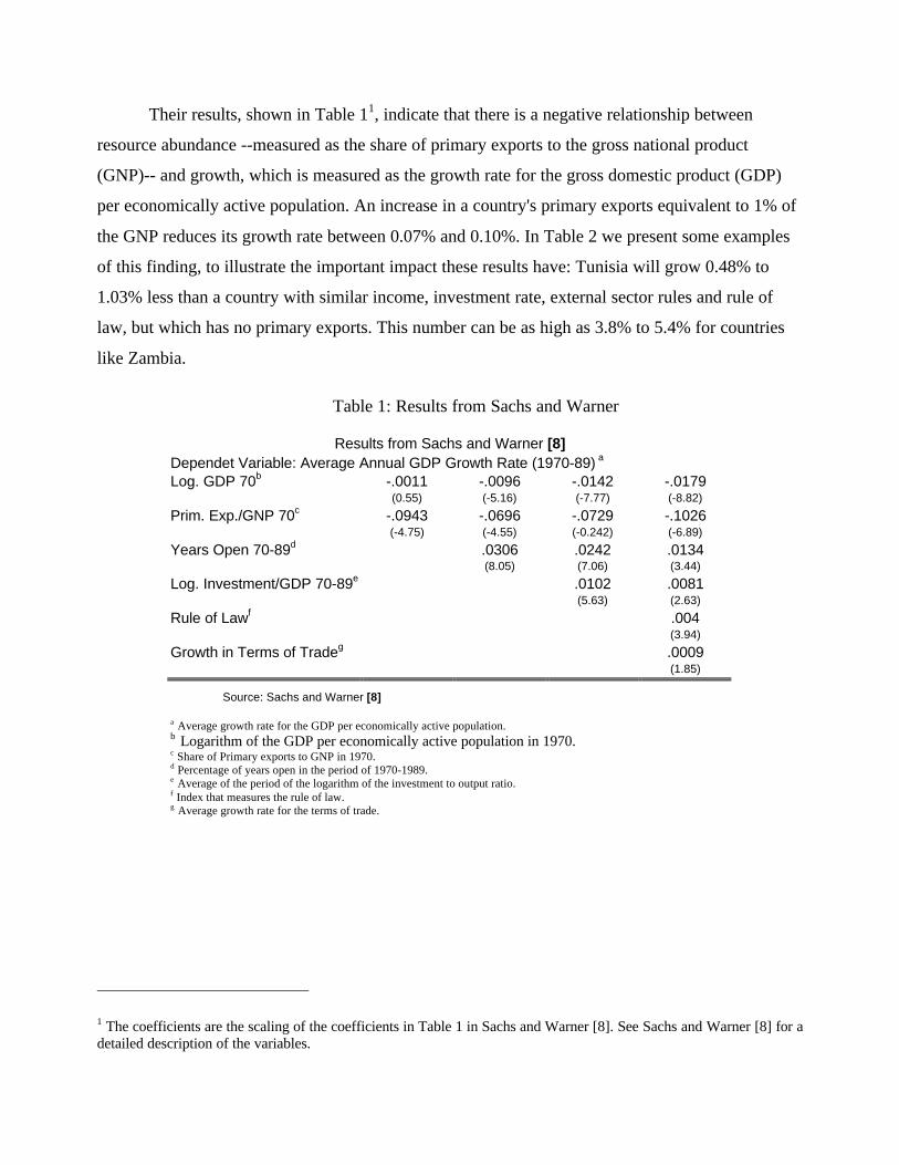
Their results, shown in Table 11, indicate that there is a negative relationship between

resource abundance --measured as the share of primary exports to the gross national product

(GNP)-- and growth, which is measured as the growth rate for the gross domestic product (GDP)

per economically active population. An increase in a country's primary exports equivalent to 1% of

the GNP reduces its growth rate between 0.07% and 0.10%. In Table 2 we present some examples

of this finding, to illustrate the important impact these results have: Tunisia will grow 0.48% to

1.03% less than a country with similar income, investment rate, external sector rules and rule of

law, but which has no primary exports. This number can be as high as 3.8% to 5.4% for countries

like Zambia.

Table 1: Results from Sachs and Warner

Results from Sachs and Warner [8]Dependet Variable: Average Annual GDP Growth Rate (1970-89) a

Log. GDP 70b -.0011 -.0096 -.0142 -.0179(0.55) (-5.16) (-7.77) (-8.82)

Prim. Exp./GNP 70c -.0943 -.0696 -.0729 -.1026(-4.75) (-4.55) (-0.242) (-6.89)

Years Open 70-89d .0306 .0242 .0134(8.05) (7.06) (3.44)

Log. Investment/GDP 70-89e .0102 .0081(5.63) (2.63)

Rule of Lawf .004(3.94)

Growth in Terms of Tradeg .0009(1.85)

Source: Sachs and Warner [8]

a Average growth rate for the GDP per economically active population.b Logarithm of the GDP per economically active population in 1970.c Share of Primary exports to GNP in 1970.d Percentage of years open in the period of 1970-1989.e Average of the period of the logarithm of the investment to output ratio.f Index that measures the rule of law.g Average growth rate for the terms of trade.

1 The coefficients are the scaling of the coefficients in Table 1 in Sachs and Warner [8]. See Sachs and Warner [8] for adetailed description of the variables.

Table 2: Sample Effects

Sample Position Country Effect1% India -0.11 to -0.16

U. S. -0.09 to -0.1350% Tunisia -0.72 to -1.03

Ecuador -0.48 to -0.8199% Malaysia -2.5 to -3.6

Guyana -3.5 to -5.0Zambia -3.8 to -5.4

Source: Authors’ calculations based on Table 1.

However, there has been recent literature suggesting evidence to the contrary. For example,

Davis [3] finds that natural-resource abundant countries have higher social indicators than other

countries, controlling by income. In addition, these countries have higher growth rates for those

indicators.

In this paper we further explore the “resource curse” using alternative approaches. We show

that the results from Sachs and Warner are not robust for small changes in the econometric

procedure. Nevertheless, the effect continues to exist in the cross-sectional, therefore, in the last

section of the paper we concentrate on explaining why it remains.

In particular, we argue that in the 70´s commodity prices were high, which led developing

countries to use them as collateral for debt2. The 80’s saw an important fall of those prices, leaving

developing countries with an important amount of debt and a low flow of foreign resources to pay

them. Thus, in the sample, the cruse (low growth) looks close to a debt-overhang problem.

The paper is organized as follows. In Section 1, we explain the problems associated we

growth regressions. Then in Section 2, we reestimate the findings of the literature, using alternative

approaches. Section 3 reviews different alternative explanations for the findings. Finally, Section 4

presents our conclusions.

2 We are not saying that there was an explicit use of them as collateral, but most creditors gave loans under theassumption that these countries will have funds to pay back based on their resource wealth.

1. The Problems of Estimating the “Resource Curse”

The empirical literature on growth starts from an estimation of the form:

tiititititi Xyyy ,,,,, lnlnln εηβα ττ +++=− −− Eq 1

where yi,t represents output for country i at period t, X represents a series of variables that explain

growth, ηi is a country specific effect, and εi,t represents the error term.

In Sachs and Warner [8], this estimation is done using the total GDP growth as an

independent variable for a cross-section of countries. These two issues --the use of total GDP and

the use of a cross-section data-- may have an impact on the coefficients estimated.

On one hand, cross-section estimators rely on the assumption that individual effects are

uncorrelated with other right-hand-side variables3. If there are some unobservable characteristics

that are correlated with the right-hand-side variables, the coefficients would be biased. As

explained in Caselli et al. [2], this assumption can be violated within the dynamic framework of a

growth regression. With a panel this problem can be solved.

On the other hand, total GDP includes the resource sector of the economy. This sector

affects total growth, especially when the share of primary exports is high. Therefore it is important

to know the behavior of the resource sector.

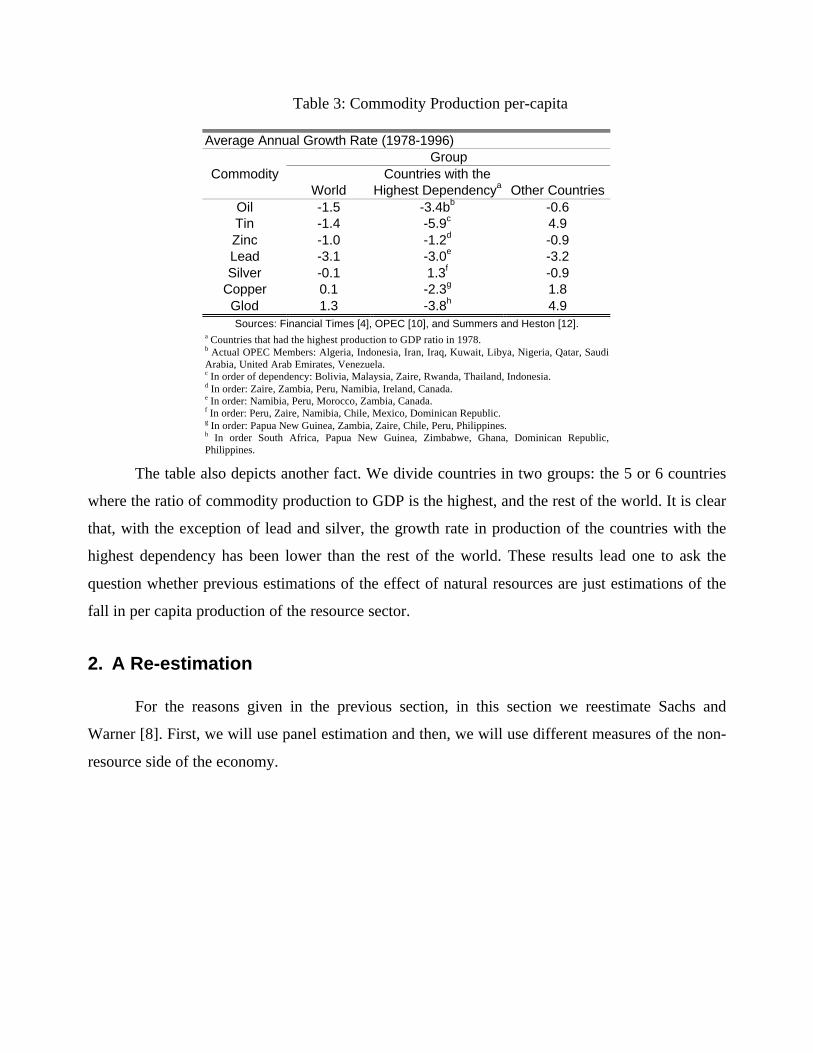
Table 3 shows the change over time of the per-capita production of 7 commodities. We use

per-capita production because this is what the left-hand side of equation (1) tries to capture. The

table indicates that the production of natural resources per capita has generally fallen. Only one

commodity (gold) has a growth rate in production greater than the average growth rate for the total

GDP (1.1%) in our sample of countries.

3 In a cross-section regression, there is only one t. Therefore, it is needed for ηi to be uncorrelated with Xi. Then, thetotal error term -ξi =ηi+εi- would be uncorrelated with Xi.

Table 3: Commodity Production per-capita

Average Annual Growth Rate (1978-1996)Group

Commodity Countries with theWorld Highest Dependencya Other Countries

Oil -1.5 -3.4bb -0.6Tin -1.4 -5.9c 4.9Zinc -1.0 -1.2d -0.9Lead -3.1 -3.0e -3.2Silver -0.1 1.3f -0.9

Copper 0.1 -2.3g 1.8Glod 1.3 -3.8h 4.9Sources: Financial Times [4], OPEC [10], and Summers and Heston [12].

a Countries that had the highest production to GDP ratio in 1978.b Actual OPEC Members: Algeria, Indonesia, Iran, Iraq, Kuwait, Libya, Nigeria, Qatar, SaudiArabia, United Arab Emirates, Venezuela.c In order of dependency: Bolivia, Malaysia, Zaire, Rwanda, Thailand, Indonesia.d In order: Zaire, Zambia, Peru, Namibia, Ireland, Canada.e In order: Namibia, Peru, Morocco, Zambia, Canada.f In order: Peru, Zaire, Namibia, Chile, Mexico, Dominican Republic.g In order: Papua New Guinea, Zambia, Zaire, Chile, Peru, Philippines.h In order South Africa, Papua New Guinea, Zimbabwe, Ghana, Dominican Republic,Philippines.

The table also depicts another fact. We divide countries in two groups: the 5 or 6 countries

where the ratio of commodity production to GDP is the highest, and the rest of the world. It is clear

that, with the exception of lead and silver, the growth rate in production of the countries with the

highest dependency has been lower than the rest of the world. These results lead one to ask the

question whether previous estimations of the effect of natural resources are just estimations of the

fall in per capita production of the resource sector.

2. A Re-estimation

For the reasons given in the previous section, in this section we reestimate Sachs and

Warner [8]. First, we will use panel estimation and then, we will use different measures of the non-

resource side of the economy.

2.1. A Panel Estimation

In order to estimate a panel, we need to obtain a different data set than Sachs and Warner

[8].4,5 Table 4 compares the result from Sachs and Warner [8]6 with the result of doing the same

cross-section analysis using our data set. It is clear the results are statistically the same.

Table 4: Sample Selection

Dependent Variable: Average Annual GDP Growth RateSachs and This

Warner SampleLog. GDP 70 -.0134 -.0135

(-7.77) (-6.698)

Prim. Exp./GNP -.0729 -.0700(-5.57) (-5.667)

Years Open 70-90 0.0242 0.0235(7.60) (6.028)

Log. Invest./GDP 70-89 0.0125 0.0140(5.63) (5.540)

N 87 79R2 0.67 0.65

t-statistics in parenthesis.

All coefficents are significant at any level

We estimate a panel using alternative data sets, one with at least 2 time elements and the

other with 4 time elements. The results are shown in Table 5. The first set of regressions, from (1.1)

to (1.3), indicates that the effect is statistically significant in the cross-section of this sub-sample

but insignificant in a panel with fixed effects. The same is done in columns (2.1) to (2.3) using the

sample with 4 time elements. This allows for the presence of more observations to calculate the

fixed effect, but there are less countries with information available to do this regression. Again, the

effect is statistically significant in the cross-section –though only at the 2.5% level-- and then

insignificant in a panel with fixed effects.

4 In Appendix A, we explain in detail some sample selection issues that drive this fact.5 In Appendix D we describe the data used for this chapter6 The reader will note that we chose regression number (1.3) of Table 1. The reason is that the Rule of Law is a “one-time” variable and therefore will not be useful for panel estimation, and that the Change in Terms of Trade was notsignificant in column (1.4).

Table 5: Effect of Natural Resources: Cross-Section vs. Panel

Dependent Variable: Average Annual GDP Growth RateUsing sample where a panel Using sample where a panelwith T=2 can be estimated with T=4 can be estimated

Panel PanelCross-Sctn Pooled Fx.Ef. Cross-Sctn Pooled Fx.Ef.

Prim. Exp./GNP -.0636* -.0565* -.0015 -.0454** -.01963 .0669***(-4.578) (-3.796) (-0.051) (-2.346) (-1.037) (1.786)

Log. GDP 70 -.0136* -.0153* -.0720* -.0154* -.0208* -.0811*(-6.687) (-5.679) (-7.995) (-6.726) (-6.776) (-7.672)

%Years Open 70-90 .0247* .0197* -.0124 .0252* .0255* .0246**(6.223) (3.954) (-1.043) (6.420) (5.597) (2.576)

Log. Invest./GDP 70-89 .0140* 0190* .0199** .0126* .0220* .0477*(5.514) (5.783) (2.003) (3.715) (5.335) (4.698)

Hausman Test 63,52 50,78F Test all ui=0 2,11 1,98

Obs 74 148 148 54 216 216N 74 74 74 54 54 54T 1 2 2 1 4 4


*,**,*** imply significant at the 1, 5 and 10% level.

0 ,00

0 ,02

0 ,04

0 ,06

0 ,08

0 ,10

0 ,12

0 ,14

0 ,00 0 ,05 0 ,10 0 ,15 0 ,20 0 ,25 0 ,30 0 ,35 0 ,40 0 ,45

Prim a ry Exports / G N P 1 9 7 0

Sta

nd

ard

Dev

iati

on

of

the

Sh

are

Figure 2: Shocks to Primary Exports

It is important to mention that the effects of the other variables do remain significant even

after the panel is done, with the expected signs and even with the expected relative size.7 The fact

that the impact of resource abundance disappears once fixed effects are introduced implies that this

variable is correlated with unobservable characteristics and therefore it disappears once fixed

effects are introduced.

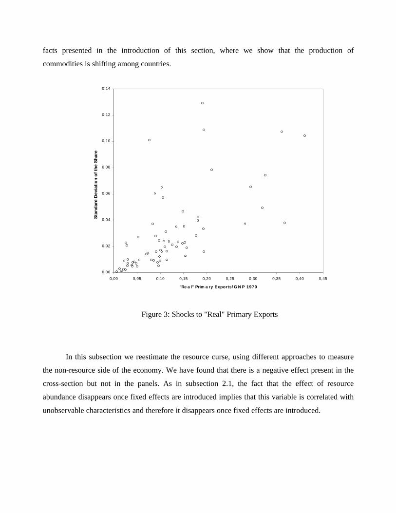
A natural concern is to ask whether we are just estimating the fixed effects of a country's

resource richness, a fact that is time invariant. In Figure 2, we show the shocks to the share

(measured through the standard deviation) compared to the share in 1970. We see that the biggest

shocks are not concentrated on the biggest producers. On the other hand, the cross-section measures

the ranking of the countries from low exporters to high exporters. In this sample it changes from

period to period.8

Summarizing, in the panel we see that there are no effects from primary exports change

through time, which cast some doubts on the validity of the conclusions derived from the cross-

sectional regressions.

2.2. Growth in the Non-Resource Sector

In this subsection we deal with the other issue related to the estimation of the effect of resource

abundance, namely the inclusion of the resource sector on the total GDP. For that purpose, we will

use alternative measures for the non-resource side of the economy. In general, the effect still

remains present for the cross-section but disappears with the fixed effects.

Throughout this section we will determine whether the effect found by Sachs and Warner

[8] on total GDP is still present in the sub-sample for which data is available for the non-resource

sector. Then, we estimate the effect on the non-resource measure of the economy. Finally, we

reestimate the effect on a panel. In this section we only present the results for the panels of 10-year

7 For example the coefficient on the lagged GDP is expected to be greater the shorter the period of time where growthis measured. For an explanation see Barro and Sala-i-Martin [1].8 See in Appendix B.

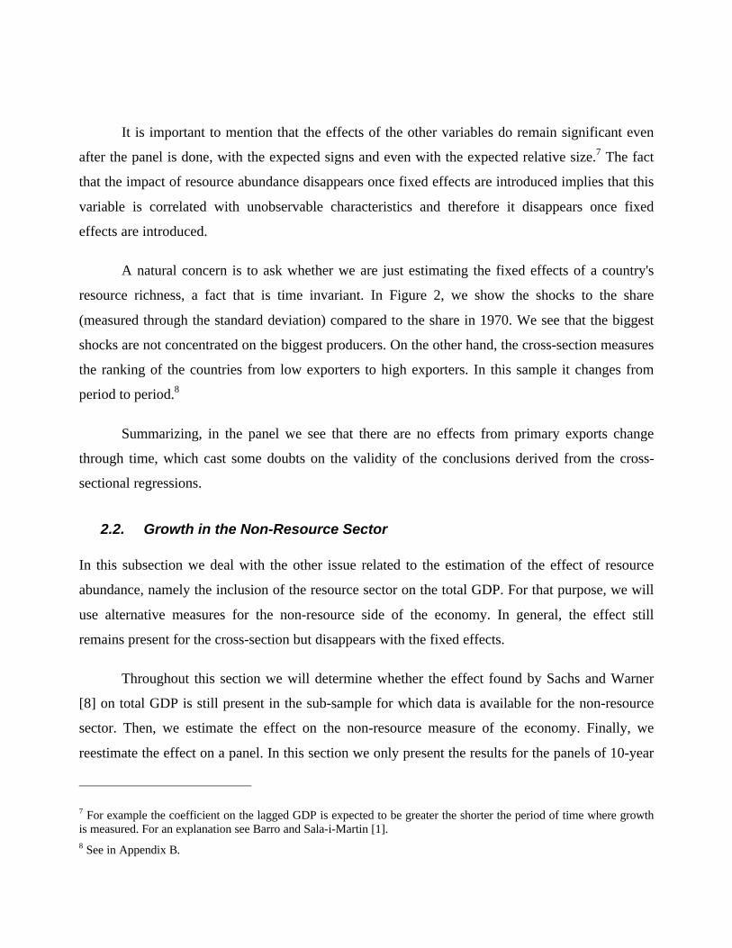
periods. The reason for this is that when a panel of 5-year periods is used the negative effect of

natural resources is lost even in the cross-sections.

For the non-resource sector of the economy we construct a measure represented by the GDP

net of resource exports. Arguably, this tends to eliminate the resource sector in those countries

where the sector is large relative to the rest of the economy.9

In Table 6, we show the cross-section results. It is clear that the effect measured by Sachs

and Warner is still present in this sub-sample. The coefficients in column (1) are actually not

significantly different from those in Table 4. Then we proceed to repeat the estimation with the

non-resource side of the economy. The results in column (2) seem to suggest that there is a negative

effect on growth in the non-resource side of the economy coming from resource abundance, similar

to the results presented in the previous subsection.

Table 6: Non-Resource Growth: Cross Section

Dependent Variable: Average Annual GDP Growth RateUsing Using

Total GDP Non-Resource GDPPrim. Exp./GNP -.0763 -.0643

(-5.677) (-4.409)

Log. GDP 70 -.0123 -.0130(-6.186) (-6.002)

Years Open 70-90 0.0233 0.0275-5.667 (6.157)

Log. Invest./GDP 70-89 0.0114 0.0090(4.583) (3.349)

N 66 66R2 0.61 0.56

t-statistics in parenthesis.All coefficients are significant at any level

In Table 7, the results from the estimation of the effect on a panel are given. As in previous

tables, we started with the cross-section to determine whether the effect is present or not. It is, but

9 See Appendix C for alternative measures of the non-resource sector. The results are qualitatively the same.

is only weakly significant.10 Again, as in the previous estimations, the effect disappears once a

panel with fixed effects is done.

Table 7: Non-Resource GDP: Cross-Section vs. Panel

Dependent Variable: Average Annual GDP Growth RatePanel

Cross-Sctn Pooled Fx.Ef.Prim. Exp./GNP -.0401** -.0351** .0061

(-2.44) (-2.061) (0.175)

Log. GDP 70 -.0126* -.0139* -.0785*(-5.796) (-4.879) (-6.468)

%Years Open 70-90 .0261* .0256* .0008(5.840) (4.607) (0.055)

Log. Invest./GDP 70-89 .0100* .'0117* .0007(3.815) (3.384) (0.046)

Hausman Test 34.58F Test all ui=0 1.27

Obs 58 116 116N 58 58T 2 2

t-statistics in parenthesis.*,**,*** imply significant at the 1, 5 and 10% level.

In the previous estimations we construct the “non-resource GDP” with the nominal share of

primary exports to GNP. If relative prices change considerably, this can affect the estimation.

Ideally, this should be corrected by using the respective deflators. However, there are no deflators

just for primary exports. For that reason, we repeat the construction of this “non-resource GDP”

taking into account changes in relative prices using the deflator for total exports compared to the

GDP deflator. It can be expected that the deflator for total exports captures the change in prices for

primary exports in countries where primary products are the main export. For purposes of

abbreviation, we will call this variable the “real” non-resource growth.11

The cross-section estimations are shown in Table 8. Column (1) shows that the effect is still

present in this sub-sample. Then, in column (2), we see that the negative effect persists on the

10 Both p-values are actually lower than 2.5%.11 This does not mean that the previous measure of “net-of-exports” GDP was nominal. It was also based on the realGDP, but without taking into account the change of relative prices inside a country.

“real” non-resource side of the economy, even with a bigger impact than in any other previous

estimation.

Table 8: "Real" Non-Resource Growth: Cross-Section



(-3.585) (-2.959)

Log. GDP 70 -.0114 -.0259(-5.617) (-5.036)

Years Open 70-90 0.0226 0.0569(-5.396) (5.377)

Log. Invest./GDP 70-89 0.0116 0.0164(4.794) (2.683)

N 61 61R2 0.61 0.51

t-statistics in parenthesis.All coefficents are significant at any level

The next step is to do the panel estimations. There are two different ways to do this

regression: one is to continue to use the nominal share of primary exports to GDP as an explanatory

variable, and the other is to use the real share. Both are used in Table 9. These alternative measures

have different interpretations: the former measures the “windfall” effect, while the latter measures

the presence and activity of a resource sector. In other words, a shock in the first one will measure a

price windfall, while a shock in the second one will measure the discovery of new reserves.

Table 9: "Real" Non-Resource GDP: Cross-Section vs. Panel


Using nominal shares Using "real" sharesCross-Sctn Pooled Fx.Ef. Pooled Fx.Ef.

Prim. Exp./GNP -.0894** -.0210 .0456 -.0378*** .0678***(-2.326) (-1.042) (1.396) (-1.705) (1.810)

Log. GDP 70 -.0249* -.0134* -.0884* -.0141* -.08271*(-4.748) (-3.956) (-8.763) (-4.190) (-8.105)

%Years Open 70-90 .0529* .0259* -.0032 .0260* -.0043(4.899) (3.809) (-0.220) (3.981) (0.295)

Log. Invest./GDP 70-89 .0172* 0100* .0101 .0107* .0061(2.870) (2.454) (0.694) (2.687) (0.4428)

Hausman Test 69,29 85.09F Test all ui=0 2.26 2.29

Obs 56 112 112 112 112N 56 56 56 56T 4 4 4 4


As in the previous regressions, we start with the cross-sections to check whether the effect is

present in the sample or not. In order to compute the real shares, a base year has to be chosen. We

chose 1970; for that reason we only need to do one cross-section. In Table 9 we see that the effect

is present in the respective cross-sections --although weak12 However, it disappears in both panels.

Moreover, the result from column (3.2) suggests a positive sign.13

As in subsection 2.1, there is the concern that once we control for changes in relative prices,

the only fixed effect is whether a country is resource rich or not, and that variable does not change

over time. For that reason, in Table 10 we show the shocks to the “real” primary exports. We see

that it is similar to Figure 2, in that the biggest shocks are not concentrated on the biggest

producers. On the other hand, there is also a shift in the ranking of the countries.14 This reflects the

12 The actual p-value is 2.4%.13 These results also appears in Appendix C.14 See Figure II in Appendix B.

facts presented in the introduction of this section, where we show that the production of

commodities is shifting among countries.

0,00

0,02

0,04

0,06

0,08

0,10

0,12

0,14

0,00 0,05 0,10 0,15 0,20 0,25 0,30 0,35 0,40 0,45

"Re a l" Prim a ry Exports/ G N P 1970

Sta

nd

ard

Dev

iati

on

of

the

Sh

are

Figure 3: Shocks to "Real" Primary Exports

In this subsection we reestimate the resource curse, using different approaches to measure

the non-resource side of the economy. We have found that there is a negative effect present in the

cross-section but not in the panels. As in subsection 2.1, the fact that the effect of resource

abundance disappears once fixed effects are introduced implies that this variable is correlated with

unobservable characteristics and therefore it disappears once fixed effects are introduced.

2.3. Dividing Resources by Origin

An important question to ask is whether the effect is the same for all kinds of primary

exports. Primary exports add agricultural, food, mineral and fuel exports together. Clearly, these are

very different products with different profitability, different behavior over time, etc. We divide

exports into account so in Table 10.

In column (2) we divide primary exports between agricultural15 and non-agricultural

exports. In column (3) we divide the non-agricultural exports into minerals and fuels. The table

shows that once exports are divided into categories, they have different effects. This reinforces the

idea that using non-resources GDP is the right approach to see the effects of resource abundance.

Table 10: Dividing Exports by Origin

Dependent Variable: Average Annual GDP Growth Rate(1) (2) (3)

Prim. Exp./GNP -.0643*(-4.409)

Agr. Exp./GNP -.0287 -.0271(-1.583) (-1.500)

Non-Agr. Exp./GNP -.1081*(-5.407)

Fuel Exp./GNP -.0669***(-1.825)

Min. Exp./GNP -.1227*(-5.414)

Log. GDP 70 -.0130* -.0121* -.0127*(-6.002) (-5.851) (-6.004)

Years Open 70-90 0.0275* 0.0247* 0.0265*(6.157) (5.717) (5.891)

Log. Invest./GDP 70-89 0.0090* 0.0113* 0.0110*(3.349) (4.273) (4.178)

N 66 66 66Hausman Espification Test 23.22 7.88

p-value 0.000 0.096

Adj. R2 0.56 0.61 0.61t-statistics in parenthesis.


15 Agricultural exports include raw materials and food.

However, this result has the same properties as all of the previous results in this research. In

Table 11, we show that, as in Section 2.1, once a panel with fixed effects is done, the effect

becomes insignificant.

Table 11: Effects of Different Resource Exports: Cross-Section vs. Panel

Dependent Variable: Average Annual GDP Growth Ratefor Non-Resource GDP

PanelCross-Sctn Pooled Fx.Ef.

(1) (2) (3)Non-Agr.Exp./GNP -.0899* -.0499* .0079

(-4.319) (0.722) (1.151)Agricultural Exp./GNP .0026 .0211 .1011

(-2.448) (-2.794) (0.227)Log.GDP -.0117* -.0128* -.0747*

(-5.814) (-4.502) (-5.965)%Years Open .0222* .0225* .0054

(5.231) (4.004) (0.339)Log.Inv./GDP .0127* .0134* .0010

(5.062) (3.874) (0.063)Hausman Test 10.23F Test all u=0 1.20Obs 58 116 116N 58 58T 2 2t-statistics in parenthesis.*,**,*** imply significant at the 1, 5 and 10% level.

3. New Dimensions of the “Curse”

The previous section makes clear that important econometric inconveniences are present in the

original formulation of the "curse". There are two striking facts that can be derived from the

previous exercises: First, in all specifications, when fixed effects are included, invariable the

natural resource curse disappears. Second, however, also in almost all specifications the curse

exists in the cross-sectional.

In this section, we tackle this second fact: why we have the effect in the cross-section. An

explanation could be that most of the source of variation is found in the cross-sectional and not on

the time series variation. A second one, already mentioned above, the coefficient in the cross-

section may be reflecting the fact that there is a correlation between omitted variables and resource

abundance. In this section we will attempt to find those omitted variables.

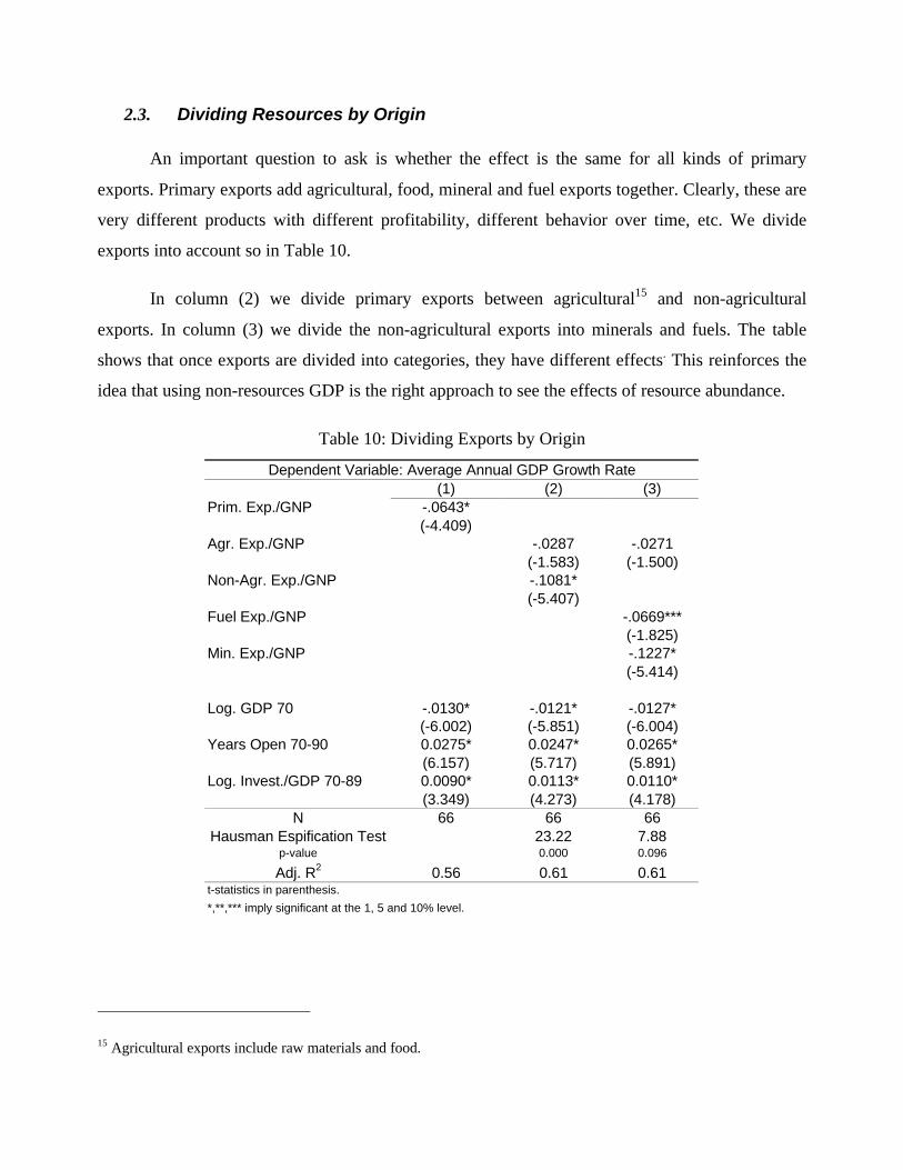
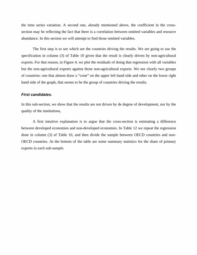
The first step is to see which are the countries driving the results. We are going to use the

specification in column (3) of Table 10 given that the result is clearly driven by non-agricultural

exports. For that reason, in Figure 4, we plot the residuals of doing that regression with all variables

but the non-agricultural exports against those non-agricultural exports. We see clearly two groups

of countries: one that almost draw a “cone” on the upper left hand side and other on the lower right

hand side of the graph, that seems to be the group of countries driving the results.

First candidates.

In this sub-section, we show that the results are not driven by de degree of development, nor by the

quality of the institutions,

A first intuitive explanation is to argue that the cross-section is estimating a difference

between developed economies and non-developed economies. In Table 12 we repeat the regression

done in column (3) of Table 10, and then divide the sample between OECD countries and non-

OECD countries. At the bottom of the table are some summary statistics for the share of primary

exports in each sub-sample.

xna70wbm0 .365397

-.043226

.023604

ALG

AUT

AUSBEL

BKF

BUR

CAN

CAR

CHL

COL

CON

CRC

DEN

DOM

ECU

EGP

SALFIN

FRA

GAB

GMB

GER

GHNGRC

GTM

GUY

HDR

HNK

IND

IDN

IRE

IVC

JAM

JAP

KNY

MDG

MLW

MLY

MLI

MTN

MAU

MEXMOR

HOL

NZL

NGA

NOR

PAKPARPHL

PORRWN

SEN

SRL

ESP

SRI

SWE

SUI

SYR

THL

TOG

TUN

TKY

UKUSA

VEN

Figure 4: Residuals and Non-Agr. Primary Exports

Non-OECD countries have a higher share of primary exports. On the other hand, this

variable does not seem to have an effect on growth in OECD countries. However, there is less

variance in the share of primary exports in OECD economies. Also we see that the variable is still

significant in non-OECD countries. Consequently, this variable is not just estimating a difference

between OECD and non-OECD economies.

An alternative is to check for variables that measure the institutional setting of a country.

We are going to focus on the variable that tries to measure the quality of bureaucracy.16 17 This

variable is measured between 0 and 6. A high value means low bureaucracy quality. Since it is

16 See Appendix F for a complete description of this variable.17 In Appendix D we repeat the regressions from this section with alternative institutional variables. These variables areintended to describe corruption, rule of law, risk of expropriation and risk of government repudiation. There is aproblem with these variables however: The methodology to construct them is the same for all. For that reason we donot introduce all of them in the same regression.

These other variables usually have the expected sign but their significance level is lower.

usually measured at a point in time, this variable can be used in panels only before the introduction

of fixed effects.

Table 12: Grouping Countries

Dependent Variable: Average Annual GDP Growth RateSample

Total OECD Non-OECD(1) (2) (3)

Non-Agr. Exp./GNP -.1081* -.0211 -.1089*(-5.407) (-0.390) (-4.116)

Agr. Exp./GNP -.0287 -.0234 -.0334(-1.583) (-1.212) (-1.352)

Log. GDP 1970 -.0121* -.0148* -.0114*(-5.851) (-4.203) (-4.898)

%Years Open 0.0247* .0161* .0284(5.717) (3.672) (4.501)

Log. Invest./GDP (Averge 79-90) 0.0113* .0132*** .0107*(4.273) (2.0271) (3.922)

N 66 21 45Adj. R2 0.61 0.73 0.62



Non Agr. Exp/GNP. Distribution in sub-sample

Sample Mean .0377 .0180 .0470

Std. Dev. .0688 .0195 .0810

Min. .0000 .0015 .0000

Max. .3654 .0590 .3654

In Table 13, we present the results from the cross-section and a panel before the fixed

effects. We also included in the table a variable that measures ethno-linguistic fractionalization.

This comes from La Porta et al. [5].18 The idea is to introduce a variable that represents an

“exogenous” institutional setting, since it is argue that rents coming from the resource sector might

have an impact on the institutional setting.

18 See Appendix D.

Table 13: Resource Abundance and Institutions

Dependent Variable: Average Annual GDP Growth Ratefor Non-Resource Growth

Cross-Section Panel (Pooled)(1.1) ´(1.2) (1.3) (2.1) ´(2.2) (2.3)

Non-Agr./GNP -.1222* -.1070* -.1040* -.0381** -.0329*** -.0220(-4.862) (-4.090) ´(-3.876) ´(-1.899) ´(-1.644) (-1.074)

Agricultural/GNP -.0470*** -.0519** -.0531** -.0461 -.0537 -.0509(-1.903) (-2.132) (-2.157) (-1.351) (-1.580) (-1.523)

Bureaucracy -.0023*** -.0025*** -.0032*** -.0035**´(-1.730) ´(-1.789) (-1.782) (-1.981)

Fractionalization -.0037 -.0173**(-0.576) (-1.994)

Bur.Non-Agr.Exp.

Bur.Agr.Exp.

Log.GDP -.0106* -.0130* -.0139* -.0141* -.0177* -.0219*(-4.449) (-4.795) (-4.363) (-4.519) (-4.809) (-5.235)

%Years .0213* .0172* .0175* .0247* .0197* .0210*(4.531) (3.337) (3.351) (4.471) (3.207) (3.459)

Log Inv./GDP .0085*** .0066 .0064 .0092*** .0070 .0069(1.952) (1.500) (1.430) (1.776) (1.334) (1.326)

Obs 53 53 53 94 94 94N 47 47 47T 2 2 2

t-statistics in parenthesis.*,**,*** imply significant at the 1, 5 and 10 % level.

In the table, we see that the effect of the primary exports disappears once institutional

variables are introduced in the panel, while it remains significant in the cross-section. The

difference between those regressions is that in the panel we allow for the fluctuations of the

primary exports over time, while in the cross-section primary exports are only going to divide the

sample into resource-rich and resource-poor countries. Therefore, the cross-section indicates that

there exists a difference between countries driven by their resource abundance.

Credit Contraints and Debt Overhang

The previous exercises indicate that neither the classification of countries into developed and

developing countries, nor the introduction of institutions change the basic result that the negative

effect is present on the cross-section. In this sub-section, we present evidence that the results on the

"curse" are mainly due to credit constraint considerations.

Giving a further look to Figure 4 indicates that the countries that are driving the result has

gone either trough an International Monetary Fund and/or a World Bank Program (including Debt

Relieves). This is confirmed by Figure 5.

xna70wbm0 .365397

-.078027

2.65553

ALG

BKFBUR

CAR

CHL

COL

CRC

DOM

ECUEGPSAL

GAB

GMB

GHNGTM

GUY

HDR

IND IDN

IVC

JAM

KNY

MDG

MLW MLY

MLI

MTN

MAU

MEX

MOR

NGA

PAK

PAR

PHLPOR

RWN

SEN

SRLSRI

SYR

THL

TOG

TUNTKY

VEN

Figure 5: Debt Growth and Resource Abundance

The previous regressions were done using the period 1970-1990. As seen in Figure 6, during

the 70´s, commodity prices were high and might have induced resource abundant countries to use

them as collateral. Then, the 80’s saw a fall in commodity prices leading to a debt crisis, which

most of these countries faced.

Figure 6 shows the evolution of commodity prices of Coal, Copper, Iron and Oil. The prices

are the nominal prices, where (for comparison reasons) they have been normalized to be equal to

100 in 1970. As can be seen, during the mid-70's the increases in commodity prices were quite

dramatic. However, all experienced drops as large as 30 percent during the 80's.

0

100

200

300

400

500

600

700

800

1970 1971 1972 1973 1974 1975 1976 1977 1978 1979 1980 1981 1982 1983 1984 1985 1986 1987 1988 1989 1990

Coal (Bitum.) Copper (elect.) Iron Ore Crude Oil

Figure 6: Commodity Prices

In Table 14, we present the change in the prices every five years. Note between 1970-1975

coal, natural gas, and iron experienced price increases that doubled their prices. Moreover, in 1975-

1980 oil and natural gas experienced their own “boom”. Coal is perhaps the most stable price in

this sample, but still its priced increase by 60 percent in the last five years of the decade of the 70's.

During the first 5 years of the 80's, coal, natural gas, iron and oil experienced an important

slowdown in their price increases to finish the decade with falls. Copper is the only exception who

suffered the fall in prices at the beginning and then a recovery.

Table 14: Price growth rate every 5 years.

Coal(Bitum.)

Nat. Gas Copper(elect.)

Iron Ore Crude Oil

1970-75 207.6% 163.2% 10.3% 98.2% 76.2%1975-80 27.3% 253.3% 57.8% 70.8% 185.6%1980-85 2.4% 57.9% -33.9% 13.2% 11.6%1985-90 -13.5% -31.9% 83.6% -26.2% -16.9%

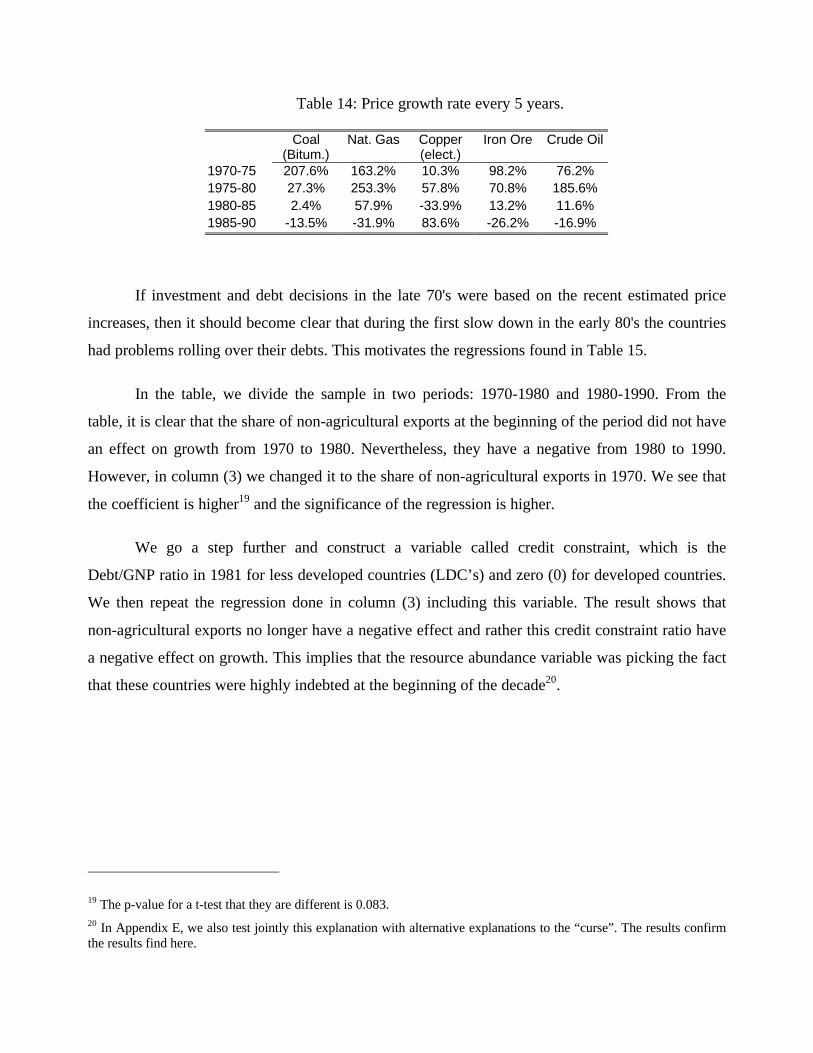
If investment and debt decisions in the late 70's were based on the recent estimated price

increases, then it should become clear that during the first slow down in the early 80's the countries

had problems rolling over their debts. This motivates the regressions found in Table 15.

In the table, we divide the sample in two periods: 1970-1980 and 1980-1990. From the

table, it is clear that the share of non-agricultural exports at the beginning of the period did not have

an effect on growth from 1970 to 1980. Nevertheless, they have a negative from 1980 to 1990.

However, in column (3) we changed it to the share of non-agricultural exports in 1970. We see that

the coefficient is higher19 and the significance of the regression is higher.

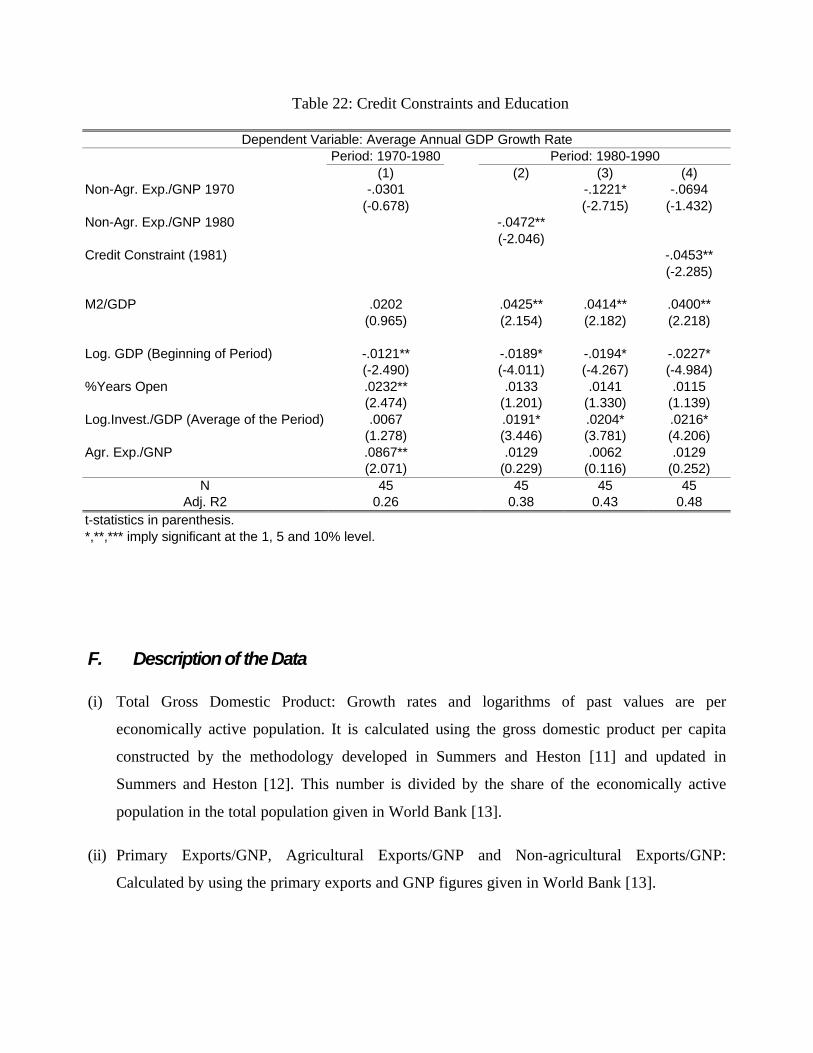
We go a step further and construct a variable called credit constraint, which is the

Debt/GNP ratio in 1981 for less developed countries (LDC’s) and zero (0) for developed countries.

We then repeat the regression done in column (3) including this variable. The result shows that

non-agricultural exports no longer have a negative effect and rather this credit constraint ratio have

a negative effect on growth. This implies that the resource abundance variable was picking the fact

that these countries were highly indebted at the beginning of the decade20.

19 The p-value for a t-test that they are different is 0.083.20 In Appendix E, we also test jointly this explanation with alternative explanations to the “curse”. The results confirmthe results find here.

Table 15: Natural Resources and Credit Constraints

Dependent Variable: Average Annual GDP Growth RatePeriod: 1970-1980 Period: 1980-1990

(1) (2) (3) (4)Non-Agr. Exp./GNP 1970 -.0525 -.1385* -.0314

(-1.256) (-3.385) (-1.452)Non-Agr. Exp./GNP 1980 -.0571*

(-2.683)Credit Constraint (1981) -.0524*

(-2.954)

Log. GDP (Beginning of Period) -.0091** -.0159* -.0171* -.0206*(-2.199) (-3.988) (-4.396) (-5.087)

%Years Open .0233* .0230** .0258* .0205**(3.166) (2.500) (2.988) (2.376)

Log.Invest./GDP (Average of the Period) .0077 .0189* .0199* .0205*(1.540) (3.700) (4.015) (4.279)

Agr. Exp./GNP .0674*** -.0366 -.0421 -.0303(1.746) (-0.790) (-0.943) (-0.701)

N 58 58 58 58Adj. R2 0.23 0.37 0.42 0.45

t-statistics in parenthesis.*,**,*** imply significant at the 1, 5 and 10 % level.

4. Conclusions

This paper considers several reasons behind the perceived poor performance of resource-

intensive economies. It reestimates the effect of natural resource abundance on growth using panel

data and improved measures of the non-resource side of the economy. We found that the effect is

always present in the cross-section data and not in the panel data. We argue that the empirical

finding in the cross sectional is due to omitted variable biases.

We thoroughly examine the possible candidates to explain the cross sectional results. We

found that degree of development and the quality of institutions were important determinants of the

growth, however, they were not the cause of the "curse"

On the other hand, we show that it is due to the fact that these countries decided to take

advantage of high commodity prices on the 70’s to use them as implicit collateral and found

themselves on a debt overhang when commodity prices fell in the 80’s.

Therefore, rather than a problem associated with the presence of natural resources, these

result seems to point out to credit market imperfections as reason for bad performance. If we think

of the commodity production of a country as part of their collateral, an increase in prices relaxes the

degree of credit constraint allowing those governments to increase their foreign debts. During the

slow down in prices and the subsequent fall, the countries were unable to continue to borrow and

had to repay part of their debts. In the end, devaluations and other contractionary measures had to

be taken to balance the current accounts, with their usual toll on growth.

Our reading of the evidence is that the curse of natural resources is not due to the particular

aspect of excessively depending on natural resources what slows down the growth rates. It is the

interaction between credit markets and a collateralizable good that is experiencing a bubble, what

causes the problems in the end. In this respect, a boom-bust cycle in a commodity price is no

different from a bubble in stock markets, as was the case of Japan, or a bubble in real estate prices,

as was in New England and Thailand.

Our interpretation is that the curse of natural resources, in this data, is another example of

the curse on asset prices bubbles. Future research should continue to explore the interaction of

credit market imperfections and the determinants of the growth. Finally, extending the present

analysis beyond the early 90's might help to unveil the relative importance of debt overhang issues

from other curses.

Appendix

A. Sample Selection

In their paper, Sachs and Warner change the base year for which the share of primary exports is

computed for 16 countries. The reasons behind those changes range from including more countries

in the sample, to including primary exports missing in National Accounts, to excluding “refinery

countries” (countries that export fuels because they import fuels to refine). As we argue in section

2, the problem that arises from those changes is that, the correct regression would be a panel.

Therefore, we will always need “beginning of period measures” of the share of primary exports.

In Table 16 we show the steps we take to solve this problem.

Table 16: Sample Selection

Dependent Variable: Average Annual GDP Growth RateThis Sample

With Modified Countries WithoutSachs and Full Prim. Exp/GDP Modified

Warner Sample can be calculated Countries(1) (2.1) (2.2) (2.3) (3.1) (3.2)

Log. GDP 70 -.0134 -.0127 -.0134 -.0121 -.0135 -.0135(-7.77) (-7.021) (-6.996) (-5.581) (-6.697) (-6.698)

Prim. Exp./GNP 70 -.0729 -.0584 -.0722 -.0700(Sachs and Warner) (-0.242) (-5.029) (-5.894) (-5.666)Prim. Exp./GNP 70 -.0344 -.0700(This Sample) (-2.970) (-5.667)Years Open 70-89 .0242 .0260 .0232 .0257 0.0235 0.0235

(7.06) (7.403) (6.234) (6.074) (6.028) (6.028)Log. Investment/GDP 70-89 .0102 .0133 .0144 .0131 0.0140 0.0140

(5.63) (6.018) (5.768) (4.616) (5.539) (5.540)N 87 95 82 82 78 79

Adj. R2 0.67 0.64 0.66 0.54 0.64 0.65t-statistics in parenthesis.


First, in column (1.1) we have the results reported by Sachs and Warner. Then, column (2.1) uses

my entire sample, but the share of primary exports, which is taken directly from Sachs and Warner

[8]. As can be seen the coefficients are not significantly different from (1.1). The same regression is

then repeated in column (2.2), but only for those countries for which we would be able to compute

the share of primary exports. Again, the coefficients are not significantly different to those in (1.1).

The next step is to do the same regression but now using my computed share of primary exports.

We see that the coefficient in the share of primary exports changes substantially. This may be due

to the presence of those countries for which Sachs and Warner changed the share of primary

exports. Therefore, in columns (3.1) and (3.2) we repeated regressions (2.2) and (2.3), respectively,

without the countries that Sachs and Warner modified. It is clear that the coefficients in (2.1) and

(3.2) are not significantly different nor are they significantly different from the original Sachs and

Warner results in (1.1). For that reason we are going to use this group of countries.

B. Change in Primary Exports

Figures I and II compare the share of primary exports and “real” primary exports to GNP in

1970 and 1980. They illustrate that there are important changes in the shares. They also illustrate,

that those changes are not only among the biggest primary exporters.

0,00

0,05

0,10

0,15

0,20

0,25

0,30

0,35

0,40

0,45

0,50

0,55

0,60

0,00 0,05 0,10 0,15 0,20 0,25 0,30 0,35 0,40 0,45 0,50 0,55 0,60

"Re a l" Prim a ry Exports/ G N P 1970

"Rea

l" P

rim

ary

Exp

ort

s/G

NP

198

0

Figure I:Change in "Real" Share of Exports

0,00

0,05

0,10

0,15

0,20

0,25

0,30

0,35

0,40

0,45

0,50

0,55

0,60

0,00 0,05 0,10 0,15 0,20 0,25 0,30 0,35 0,40 0,45 0,50 0,55 0,60

Primary Exports 1970

Pri

mar

y E

xpo

rts

1980

Figure II: Change in the Share of Exports

C. Alternative measure of Non-Resource GDP.

The World Bank provides data on some sectors of countries' economies, in particular

manufacturing and services. In this subsection we estimate the effect of resource exports on the

combined GDP --as a proxy for the non-resource sector.

In Table 17, we present the results from a cross-section of countries. From the result for the

total GDP, we see that the result from Sachs and Warner is present in this regression. In the

sectorial data, we find that we still get a negative effect from primary exports.21 This seems to

suggest that there is the predicted negative effect.

Table 17: Manufacturing and Services GDP



(-4.790) (-2.744)

Log. GDP 70 -.0157 -.0108(-7.061) (-2.418)

Years Open 70-90 .0302 .0316(6.781) (3.363)

Log. Invest./GDP 70-89 .0143 .0131(4.967) (2.239)

N 54 54R2 0.72 0.35



In Table 18, we proceed to reestimate the effect with a panel. It indicates that once a panel

with fixed effects is done, the negative effect of primary exports is lost. Consequently, it seems that

there is no evidence of a negative effect from resource abundance in the growth of non-resource

sectors.

21 This result is also found by Sachs and Warner [8] in their paper. See Table VIII, column (8.2). However, in Manzano[6], the sectors are divided looking for evidence of “Dutch Diesease” and it is found that the negative effect is found onthe service sector and not in the manufacturing sector, contrary to what it is expected from the “Dutch Disease”literature.

Table 18: Manufacturing and Service GDP: Cross-Section vs. Panel


Cross-Sctn Pooled Fx.Ef.Prim. Exp./GNP -.0780* -.0430** .0882***

(-2.860) (-1.958) (1.815)

Log. GDP 70 -.0080*** -.0152* -.0619*(-1.835) (-4.160) (-5.412)

%Years Open 70-90 .0309* .0290* -.0146(3.261) (3.819) (-0.886)

Log. Invest./GDP 70-89 .0001 .0101 -.0076(0.195) (1.439) (-0.483)

Hausman Test 50.02F Test all ui=0 2.27

Obs 48 96 96N 48 48T 2 2



D. Alternative Institutional Variables

In Table 19, we repeat the estimation done in the cross-sections of Table 13, with other

institutional variables. These variables represent a corruption index, a rule of law index, an index

that tries to capture the risk of government repudiation, and another the tries to capture the

expropriation risk.22 It is clear that these variables are not statistically significant, while the non-

agricultural resource abundance variable continues to be significant in the regression.

22 See Appendix E for a complete description of the variables.

Table 19: Alternative Institutional Variables

Dependent Variable: Average Annual GDP Growth Ratefor Non-Resource Growth.

Cross-Section(1.1) (1.2) (2.1) (2.2) (3.1) (3.2) (4.1) (4.2)

Non-Agr./GNP -.1129* -.1110* -.1079* -.1053* -.1242* -.1246* -.1275* -.1282*(-3.483) (-3.171) (-3.307) (-2.949) (-3.782) (-3.436) (-3.925) (-3.546)

Corruption .0011 .0012(0.7089) (0.7709)

Rule of Law .0025 .0026(-1.424) (1.417)

Gov. Repudiation 0.0015 .0015(0.903) (.8944)

Exp. Risk .0007 .0007(.4501) (.4340)

Fractionalization -.0027 -.0034 .0004 .0007(-0.362) (-0.471) (.0396) (.0710)

Log.GDP -.0118* -.0124* -.0135* -.0144* -.0089* -.0087*** -.0090* -.0087(-3.887) (-3.579) (-3.887) (-3.665) (-2.934) (-1.766) (-2.883) (-1.711)

%Years .0195* .0197* 0.0178* .0181* .0198* .0198* .0215* .0215(3.866) (3.838) (3.645) (3.622) (3.078) (3.039) (3.433) (3.384)

Log Inv./GDP .0074 .0072 .0058 .0056 .0075 .0075 .0074 .0075(1.602) (1.524) (-1.139) (1.059) 1.350 (1.2717) (1.319) (1.220)

Agricultural/GNP -.0555 -.0584 -.0491 -.0500 -.0485 -.0482 -.0513 -.0508(-1.670) (-1.671) (-1.546) (-1.517) (-1.195) (-1.092) (-1.275) (-1.146)

N 53 53 53 53 36 36 36 36Adj. R 0.57 0.57 0.59 0.58 0.55 0.53 0.54 0.53



E. Robustness Check.

In this appendix we test together our reading of the resource “curse” and alternative

explanations to it. In Table 20, we present the result of repeating the regressions found on Table 15,

but adding institutional performance. The degree of financial development should be correlated

with rule of law and the quality of the bureaucracy. In this regression, we test for the robustness in

our results regarding the credit constraint results.

Table 20: Credit Constraints and Institutions


(1) (2) (3) (4)Non-Agr. Exp./GNP 1970 -.1032** -.0848*** -.0537

(-1.827) (-1.842) (-1.144)Non-Agr. Exp./GNP 1980 -.0430**

(-2.090)Credit Constraint (1981) -.0405**

(-2.027)

Bureaucracy .0024 .0029 .0032c .0024(0.893) (1.272) (1.403) (1.097)

Log. GDP (Beginning of Period) -.0095*** -.0243* -.0233* -.0269*(-1.733) (-5.434) (-5.151) (-5.717)

%Years Open .0204** .0197** .0202** .0190**(2.198) (2.358) (2.398) (2.338)

Log.Invest./GDP (Average of the Period) .0022 .0144 .0127*** .0149**(0.262) (2.134) (1.916) (2.298)

Agr. Exp./GNP .0368 -.1161* -.1062** -.0958**(0.721) (-2.777) (-2.554) (-2.373)

N 47 47 47 47Adj. R2 0.25 0.44 0.43 0.47


As can be seen, the resource curse survives the inclusion of bureaucracy. The same

conclusion as before is found: The effect of primary exports disappears when credit constraint

variables are included in the regression.

A second robustness check is to find how sensitive the results are to other variables that

explain growth. In particular, resource abundance could be negatively correlated with many

different variables that are used to explain growth23. In table 21, we test for one of them, Education.

Which, indeed, it is negatively correlated with resource abundance. As seen in the Table the results

from Table 15 do not change with the introduction of it.

23 We thank Bill Easterly for pointing us this fact.

Table 21: Credit Constraints and Education


(1) (2) (3) (4)Non-Agr. Exp./GNP 1970 -.0300 -.1411* -.0720

(-0.697) (-3.145) (-1.420)Non-Agr. Exp./GNP 1980 -.0786*


(-2.512)

Sec. Enrollment (Beginning of Per.) .0040 .0057 -.0015 .00357(0.861) (1.076) (-0.287) (0.673)


%Years Open .0255* .0243* .0269* .0224**(3.356) (2.671) (3.013) (2.594)

Log.Invest./GDP (Average of the Period) .0059 .0147** .0184* .0171*(1.540) (2.474) (3.005) (2.924)

Agr. Exp./GNP .0645 -.0554 -.0365 -.0360(1.653) (-1.151) (-0.789) (-0.820)

N 55 55 55 55Adj. R2 0.35 0.36 0.36 0.43


In Table 22 we test for another variable used to explain growth, financial development,

measured as M2 to GDP Ratio. It is also negatively correlated with resource abundance. As seen in

the Table financial development is indeed significant, and has a positive effect on growth.

However, the results from Table 15 still do not change with the introduction of it. This exercise can

be repeated with several other variables standard in growth regressions and the results hold.

Table 22: Credit Constraints and Education


(1) (2) (3) (4)Non-Agr. Exp./GNP 1970 -.0301 -.1221* -.0694

(-0.678) (-2.715) (-1.432)Non-Agr. Exp./GNP 1980 -.0472**


(-2.285)

M2/GDP .0202 .0425** .0414** .0400**(0.965) (2.154) (2.182) (2.218)


%Years Open .0232** .0133 .0141 .0115(2.474) (1.201) (1.330) (1.139)

Log.Invest./GDP (Average of the Period) .0067 .0191* .0204* .0216*(1.278) (3.446) (3.781) (4.206)

Agr. Exp./GNP .0867** .0129 .0062 .0129(2.071) (0.229) (0.116) (0.252)

N 45 45 45 45Adj. R2 0.26 0.38 0.43 0.48


F. Description of the Data

(i) Total Gross Domestic Product: Growth rates and logarithms of past values are per

economically active population. It is calculated using the gross domestic product per capita

constructed by the methodology developed in Summers and Heston [11] and updated in

Summers and Heston [12]. This number is divided by the share of the economically active

population in the total population given in World Bank [13].

(ii) Primary Exports/GNP, Agricultural Exports/GNP and Non-agricultural Exports/GNP:

Calculated by using the primary exports and GNP figures given in World Bank [13].

(iii) Years Open: Percentage of years open in the period of reference. The number of years open is

based on the criteria used in Sachs and Warner [6] to determine whether a country is open or

not in a certain year.

(iv) Investment/GDP: Calculated using the values provided by Summers and Heston [12].

(v) Manufacturing and Services GDP: calculated using the figures of GDP described in (i) and the

shares of the sectors given in World Bank [13].

(vi) Non-Resource Sector: Calculated using the data described on (i) and (ii).

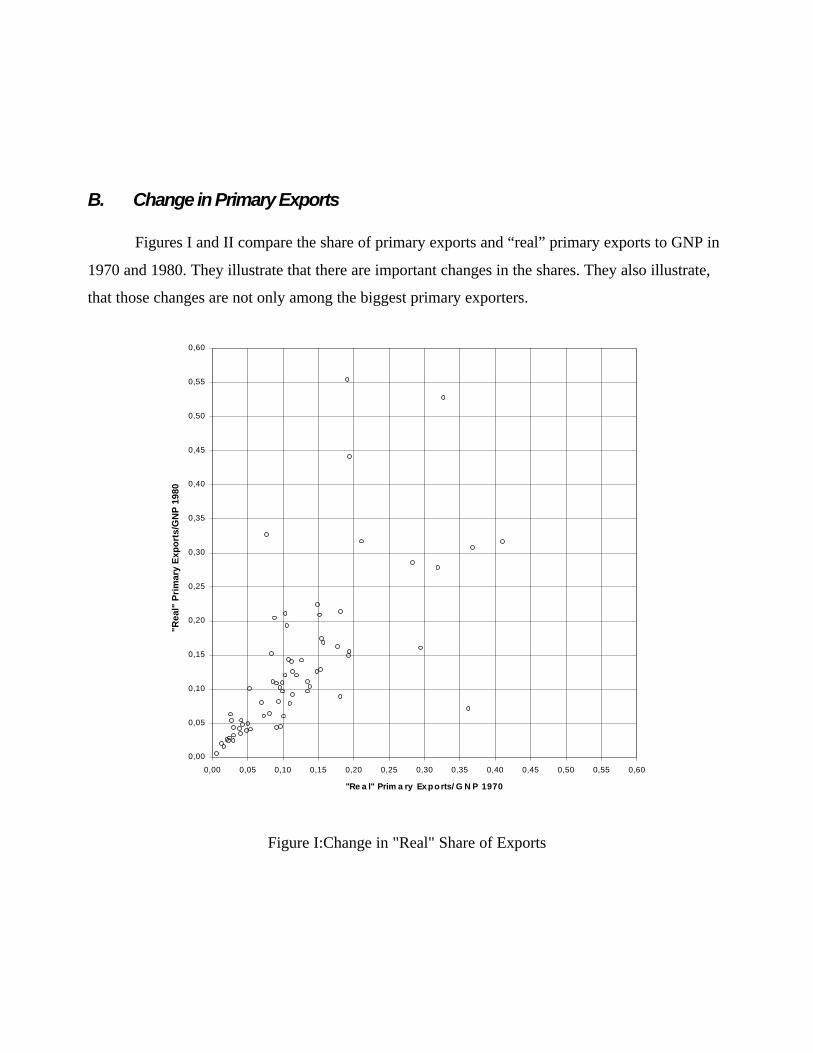
(vii) “Real” Non-Resource Sector and “Real” Primary Exports Share: calculated using the data

described in (i) and (ii) and the ratio of the deflators for merchandise exports and GDP given in

World Bank [13].

(viii) Bureaucracy: Calculated using the Index of Bureaucracy Quality from Keefer, Philip and

Stephen Knac (1995), ``Institutions and Economic Policy: Cross-Country Tests Using

Alternative Institutional Measures'', Economics and Politics, VII, 207-227 (cited by Sachs and

Warner [9]). The variable in this paper is equal to 6 (maximum possible value) minus the

actual value of the index. A lower value means a higher quality of bureaucracy.

(ix) Fractionalization: Ethno-linguistic fractionalization. Taken from La Porta et al. [5].

(x) Credit Rationing: Total External Debt divided by the GNP for the countries which this ratio is

available in World Bank [13]. These countries are all less developed countries. For OECD’s

countries this variable was set to zero (0).

(xi) Secondary Enrollment: Percentage of the age group attending secondary school. Taken from

World Bank [13].

References

[1] Barro, Robert and Xavier Sala-i-Martin (1995), Economic Growth, McGraw-Hill, NewYork.

[2] Caselli, Franceso, Gerardo Esquivel and Fernando Lefort (forthcoming), "Reopening theConvergence Debate: A New Look at the Cross-County Growth Empirics'', Journal ofEconomic Growth.

[3] Davis Davis, Graham (1995), "Learning to Love the Dutch Disease: Evidence fromMineral Economies'', World Development, 23, 1765-1779.

[4] Financial Times (various years), Financial Times International Yearbooks: Mining,Longmann, Essex.

[5] La Porta, Rafael, Florencio Lopez-de-Silanes, Andrei Shleifer and Robert Vishny(1998), "The Quality of Government'', Mimeo, Harvard University.

[6] Manzano, O., Natural Resources, Taxation and Public Policy, Dissertation submitted tothe Department of Economics at MIT as a part of the requirements to the fulfillment ofthe Ph.D. in Economics, MIT, Cambridge.

[7] Sachs, Jeffrey and Andrew Warner (1995a), "Economic Reform and the Process ofGlobal Integration'', Brookings Papers on Economic Activity, 25th anniversary issue, 1-118.

[8] Sachs, Jeffrey and Andrew Warner, (1997a), "Natural Resource Abundance andEconomic Growth'', mimeo, Center for International Development, Harvard University.

[9] Sachs, Jeffrey and Andrew Warner (1997b), Natural Resource Abundance andEconomic Growth, Data set available at http://www.cid.harvard.edu/data.htm

[10] OPEC (various years), Annual Statistical Bulletin, The Secretariat, Organization ofPetroleum Exporting Countries, Vienna.

[11] Summers, Robert and Alan Heston (1991), "The Penn World Table (Mark 5): AnExpanded Set of International Comparisons'', Quarterly Journal of Economics, 106,327-368.

[12] Summers, Robert and Alan Heston (1995), The Penn World Table (Mark 5.6), Dataset available at http://pwt.econ.upenn.edu/

[13] World Bank (1999), World Development Indicators, (CD-ROM Data), WashingtonD.C.

Date post:	14-Mar-2018
Category:	Documents
Upload:	vuongnhi
View:	217 times
Download:	1 times

Abstract - MITweb.mit.edu/rigobon/www/Robertos_Web_Page/Research_files/resour… · Resource Curse...

Documents