ABSTRACT SMITH, KARA ANN. The Role of the Dominant Modes of Climate Variability over Eastern Africa in Modulating the Hydrology of Lake Victoria. (Under the direction of Fredrick Semazzi). Previous water budget studies over the Lake Victoria basin have shown that there is near balance between rainfall and evaporation and that the variability of Lake Victoria levels is determined virtually entirely by changes in rainfall since evaporation is nearly constant. It is also well known that the variability of rainfall over East Africa is dominated by ENSO. However, the dipole mode is the second most dominant rainfall climate mode also accounts for significant variability across the region. The hydrologic adjustment time of the lake is also on a decadal scale. Based on this knowledge, we hypothesize that ENSO dominates the variability of Lake Victoria levels. We further hypothesize that the dipole mode and hydrologic adjustment also play significant roles but we are uncertain which of these two is more significant. The rela- tionship between the ENSO and dipole mode with Lake Victoria levels is nonlinear and a key objective in this study is to estimate the relative contributions of these modes in modulating Lake Victoria levels to test our hypothesis. We find that the sudden significant increase in lake levels from 1961-64 was mainly caused by consistent above average precipitation during those years, while the decline from 1965-2005 was due to the lake reaching a new equilibrium level. The first EOF mode of annual precip- itation variability (ENSO) accounts for the highest impact on the annual variability of Lake Victoria levels. While the second annual EOF mode accounts for approximately 10 percent of the variability, its affect on the variability of lake levels is nearly negligible because the loadings are very small over the lake.
Transcript
ABSTRACT
SMITH, KARA ANN. The Role of the Dominant Modes of Climate Variability over EasternAfrica in Modulating the Hydrology of Lake Victoria. (Under the direction of FredrickSemazzi).
Previous water budget studies over the Lake Victoria basin have shown that there is near
balance between rainfall and evaporation and that the variability of Lake Victoria levels is
determined virtually entirely by changes in rainfall since evaporation is nearly constant. It
is also well known that the variability of rainfall over East Africa is dominated by ENSO.
However, the dipole mode is the second most dominant rainfall climate mode also accounts for
significant variability across the region. The hydrologic adjustment time of the lake is also on
a decadal scale.
Based on this knowledge, we hypothesize that ENSO dominates the variability of Lake
Victoria levels. We further hypothesize that the dipole mode and hydrologic adjustment also
play significant roles but we are uncertain which of these two is more significant. The rela-
tionship between the ENSO and dipole mode with Lake Victoria levels is nonlinear and a key
objective in this study is to estimate the relative contributions of these modes in modulating
Lake Victoria levels to test our hypothesis.
We find that the sudden significant increase in lake levels from 1961-64 was mainly caused
by consistent above average precipitation during those years, while the decline from 1965-2005
was due to the lake reaching a new equilibrium level. The first EOF mode of annual precip-
itation variability (ENSO) accounts for the highest impact on the annual variability of Lake
Victoria levels. While the second annual EOF mode accounts for approximately 10 percent
of the variability, its affect on the variability of lake levels is nearly negligible because the
loadings are very small over the lake.
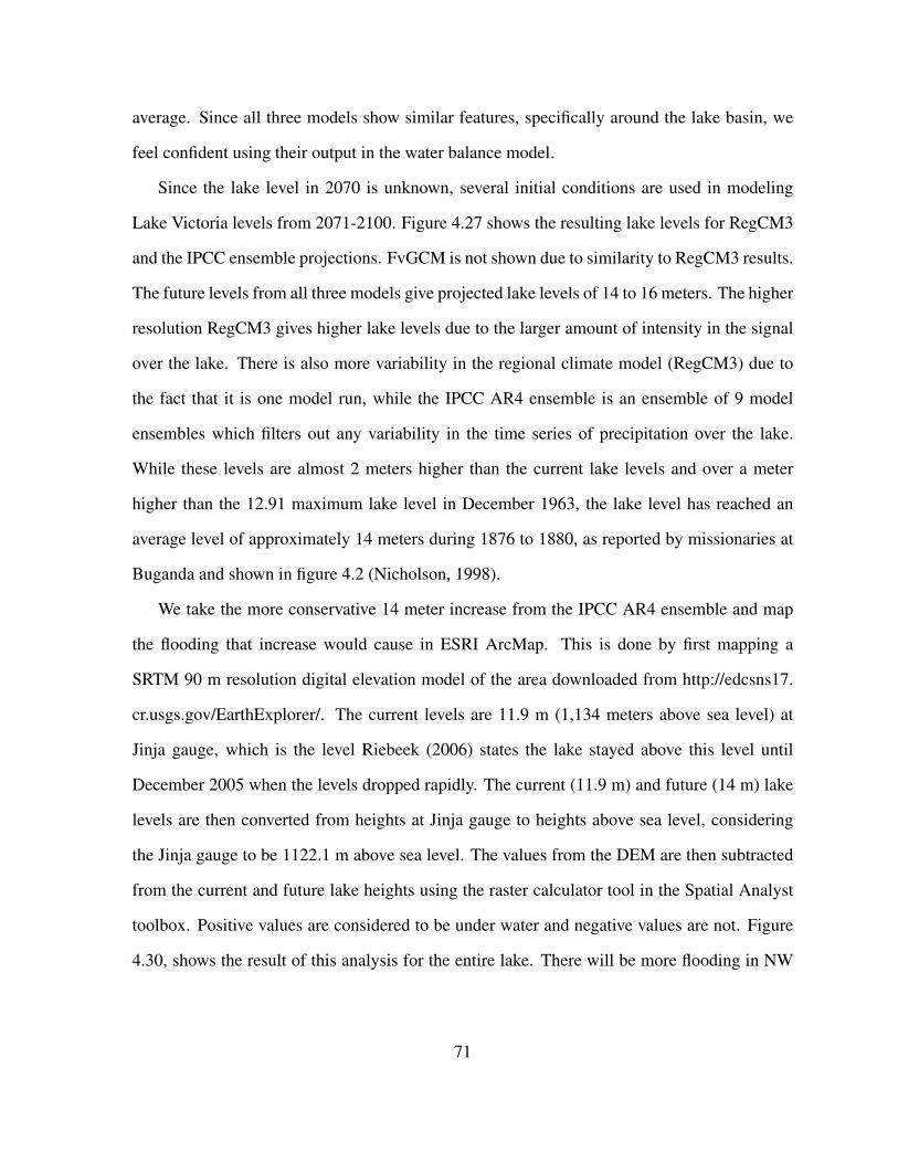
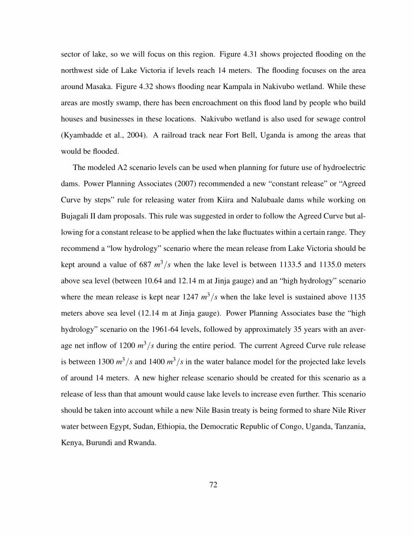
Lake Victoria levels could reach 14 meters under IPCC AR4 A2 scenario projections. We
map the potential flooding from these increased levels using GIS. This information is poten-
tially highly valuable in assessing future use of hydroelectric dams and other applications such
as land use and infrastructure planning over the Lake Victoria basin.
The annual variability in precipitation in terms of the seasonal variability from station
gauge precipitation over Uganda, Kenya and Tanzania is investigated by performing seasonal
EOF analysis on station gauge precipitation for the October-December (OND), March-May
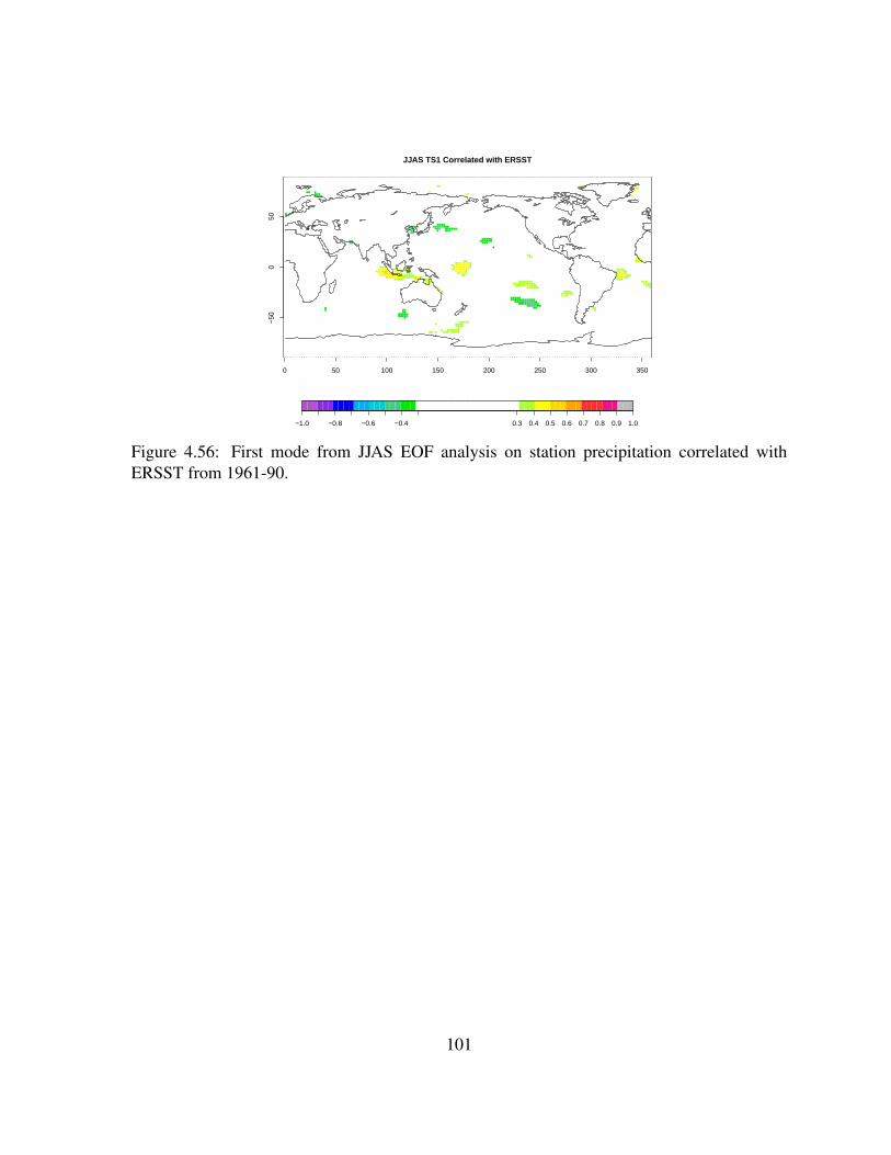
(MAM), January-February (JF) and June-September (JJAS) seasons. The EOF time series of
the dominant modes are correlated with SST anomalies for each season to help determine their
sources of variability. The first annual mode is correlated with the first modes of OND and
MAM seasons, while the second mode is correlated with the second modes of MAM and JJAS
seasons.
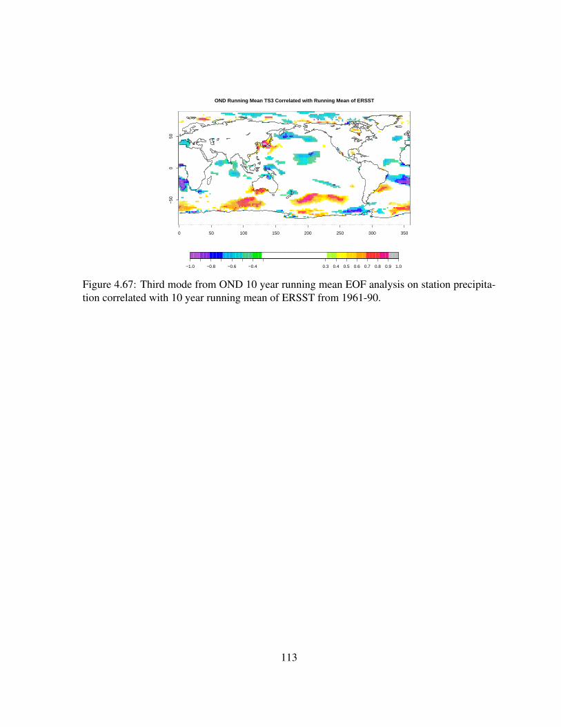
We then perform EOF analysis on a ten year running mean of 1961-90 OND season station
precipitation to investigate decadal variability. Correlation of the time series of the first EOF
mode with SST anomalies gives a ‘ENSO-like’ signal pattern consistent with recent studies.
We recommend that there is a definite need for sustained and improved monitoring of the
lake and its basin, to compile high quality monthly observations for all the factors in the water
balance model including information on water taken from the lake and its tributaries for human
use. We further recommend the use of a dynamical hydrological model for use in projections
of lake levels for climate change scenarios. Such a model would have more reliability outside
of the regimes under which the model used in this study was calibrated. Future studies would
benefit from an estimation of the cascade of uncertainty over the entire chain of steps involved
from data collected to impact modeling.
The Role of the Dominant Modes of Climate Variability over Eastern Africa in Modulating
ERSST: Extended Reconstruction Sea Surface Temperature
FFT: Fast Fourier Transform
FvGCM: NASA Finite Volume Global Climate Model
GIS: Geographic Information System
IOZM: Indian Ocean Zonal Mode
IPCC: International Panel on Climate Change
JF: January-February season
JJAS: June-September season
MAM: March-May season
NBS: Net Basin Supply
OND: October-November season
RegCM3: ICTP REGional Climate Model system version 3
SO: Southern Oscillation
SOI: Southern Oscillation Index
SSTs: Sea Surface Temperatures
TS: Time Series
WBM: Water Balance Model
xvi
Chapter 1
Introduction
Lake Victoria and Nile River Basins
Lake Victoria is one of the sources of Nile River which is the lifeblood of the ten African
nations of Egypt, Sudan, Rwanda, Uganda, Tanzania, Zaire, Ethiopia, Kenya, Eritrea, and Bu-
rundi. With a population of less than 10 million, the great ancient civilizations along the Nile
valley relied on the abundance of Niles’s water supply to thrive. Despite the low population
at that time, it is believed that failure of the Nile discharge to deliver sufficient water due to
climatic fluctuations may have resulted in the collapse of several ancient Egyptian dynasties
of the great Pharaohs. The Nile has annual flow in normal years of about 84 billion cubic
meters at Aswan in southern Egypt. Of this, about 85 percent is from the Blue Nile, the At-
bara and the Sobat rivers, originating in the Ethiopian highlands. The rest originates from
the Great Lakes region of which Lake Victoria is the most important source. Records show
that from 1870 to 1899, the average annual flow at Aswan was 110 bcm, and declined to 83
bcm from 1899 to 1954 and 81.5 bcm from 1954 to 1988. Consequently, the demand for ac-
curate projections of future fluctuations in the Nile flow and its sources has become a matter
of very high priority for the Nile basin countries. The Anglo-Italian Agreement of 1891 and
subsequent treaties are the basis for the sharing of the river’s water by the ten countries. The
main treaties include, the Anglo-Italian Protocol of April 15, 1891; the Treaty between Great
Britain and Ethiopia of May 15, 1902; the Tripartite (Britain-France-Italy) Treaty of Decem-
ber 13, 1906; the Agreement between Egypt and Anglo-Egyptian Sudan of 7th May 1929; &
the post-colonial agreements (the 1959 Nile Agreement between the Sudan and Egypt). These
agreements and the latest plans to redress the Nile water treaties do not adequately take into
account the projected impacts of climate change on water supplies. This is a serious shortcom-
ing since some estimates indicate that climate changes in the next few decades could reduce
run-off over the arid regions by up to 40-70%. Compounding the problem even further, current
estimates of climate change which are primarily based on global climate models do not have
sufficient geographical detail required for the application of hydrological models at catchments
spatial scales. There are significant socio-political issues associated with water resources over
the Lake Victoria Basin, yet currently there is limited science behind water policy within coun-
tries of the region. Its water sharing also presents significant trans-boundary environmental
challenges. Basic research addressing variability and predictability of river basin regimes, and
implications for major climatic phenomena such as climate change, El Nino and other complex
climatic phenomena on watersheds is needed. The science is still in its infancy as the transla-
tion even of such a major phenomenon as an El Nino into its implications for a watershed is
complex and for lesser climatic phenomena even more difficult. The science and data are both
clearly inadequate.
ENSO and Dipole Climate Modes
It is well known that El Niño-Southern Oscillation (ENSO) and the Indian Ocean Zonal
Mode (IOZM) dominate the interannual climate variability of Eastern Africa (Ogallo, 1979;
Ogallo et al., 1988; Nyenzi, 1992; Nicholson, 1996; Latif et al., 1998). More recently Schreck
2
and Semazzi (2004) unveiled a new mode represented by the second most important regional
precipitation EOF mode characterized by decadal variability and a dipole rainfall loading pat-
tern (Fig. 1.1). The spatial distribution of rainfall over Lake Victoria Basin (LVB) is com-
plex as shown in figure 1.2. It consists of a wave-like dry-wet-dry-wet climatological rainfall
pattern. During previous ten years significant progress has been made in understanding the
physical mechanisms which determine its characteristics (Anyah et al., 2009; Bowden and Se-
mazzi, 2007; Anyah and Semazzi, 2007; Anyah and Semazzi, 2006; Anyah et al., 2006; Anyah
and Semazzi, 2004; Song et al., 2004). Over the eastern sector of the lake rainfall is mini-
mum & less than 800mm per year (Asnani, 1993, 2005); over the western sector of the lake
rainfall is maximum and over 2000 mm per year; there is a well-marked rainfall maximum
(more than 1500mm) over land immediately to the east the lake; and a rainfall minimum (less
than 1000mm) immediately to the west of Lake Victoria. This climatic pattern, its variabil-
ity & associated atmospheric & marine conditions determine the performance of the primary
social-economic activities across the Lake Victoria basin including agriculture, fisheries, hy-
droelectric power generation. Global climate models with resolution of 100km and coarse
cannot resolve the important features of the distribution of rainfall in figure 1.2 and regional
climate models with resolution of 10s of km in resolution would be required. Equally impor-
tant, these models should adequately represent several critical mechanisms including basin-
scale orographic-dynamic forcing, interaction of large scale prevailing flow & lake-land breeze
mesoscale circulation, and the role of lake surface temperature gradient.
3
Figure 1.1: (left top) EOF1 based on CMAP rainfall data set (1979-1999); (left bottom) EOF1time series, red line corresponds to station gauge EOF 1, solid blue is East African regionalCMAP EOF1; (top right) EOF2 loading based on CMAP rainfall data set (1979-1999); (rightbottom) red line corresponds to eastern Africa CMAP EOF2, solid blue is CMAP global EOF3,and dotted is global average surface temperature time series based on HadCRUT data set, anindicator of global warming.
4
Figure 1.2: Observed annual rainfall (mm). Purple circles are locations for Bukoba and Mu-soma.
Hydroelectric Power Plants
Nalubaale Dam (originally called Owen Falls Dam), located at the Jinja Lake Victoria
coastal city in Uganda (at source of the Nile), was the first major hydroelectric plant to be
constructed in Uganda. It was opened in 1959 to provide hydroelectric power for the region.
Kiira Dam was commissioned in 2000 to generate more electricity from the excess water being
spilled by the sluices of Nalubaale (Kull, 2006(a). The Bujagali dam, 250 Megawatts (MW),
is expected to be commissioned in 2011. The Murchison Falls dam in Uganda and several
other plants in Sudan are in the planning phase. The flow of the White Nile, and hence the
productivity of these dams are primarily determined by the level of Lake Victoria (Fig. 1.3).
The temporal variability of the level of the lake is in turn primarily determined by the rainfall
5
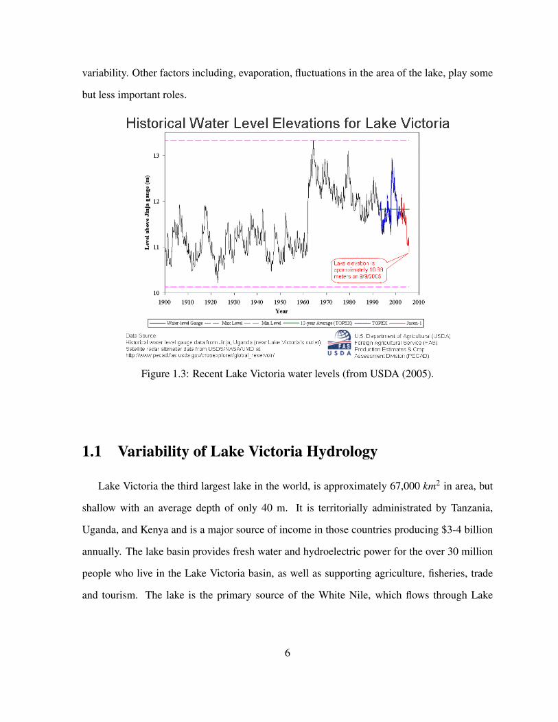
variability. Other factors including, evaporation, fluctuations in the area of the lake, play some
but less important roles.
Figure 1.3: Recent Lake Victoria water levels (from USDA (2005).
1.1 Variability of Lake Victoria Hydrology
Lake Victoria the third largest lake in the world, is approximately 67,000 km2 in area, but
shallow with an average depth of only 40 m. It is territorially administrated by Tanzania,
Uganda, and Kenya and is a major source of income in those countries producing $3-4 billion
annually. The lake basin provides fresh water and hydroelectric power for the over 30 million
people who live in the Lake Victoria basin, as well as supporting agriculture, fisheries, trade
and tourism. The lake is the primary source of the White Nile, which flows through Lake
6
Kyoga in Uganda and Lake Albert into Sudan where it joins with the Blue Nile at Khartoum
to form the Nile River, which supports the livelihood of over 300 million people. The climate
of the lake basin is dominated by the bimodal signature of the intertropical convergence zone
(ITCZ).
After a long period of near constant levels in the early part of this century, Lake Victoria
levels rose by almost 2.5 m between 1961 and 1964. This has been explained by a strong
Indian Ocean Dipole in 1961 and unusually high precipitation in East Africa in late 1961 and
1962 (Piper et al., 1986; Sene and Plinston, 1994; Kite, 1981). The lake levels remained above
the previous average, decreasing slightly over time until 2002 when the rate of decrease more
rapidly (Fig. 1.3). From late 2003 through 2005, Lake Victoria’s water level dropped over 1.1
m from it’s 10 year average (Fig. 1.3). As of December 2005, it was approximately 10.69 m,
reaching the lowest level since 1951 (USDA, 2005). Various studies have investigated this drop
(Kull, 2006(a,(; Sutcliffe and Petersen, 2007; Mangeni, 2006), attributing the drop to various
combinations of over-release from Nalubaale and Kiira dams and a drought which affected the
area for several years. While there is not enough data currently to study this drop in lake levels,
we plan to study the slow drop from 1965-2005 and the sudden increase in levels from 1961-
64 which preceded it. These abrupt changes in level and the resulting changes in lake outflow
have important impacts on the hydrology of the Nile River and hydropower generation at Jinja,
Uganda.
In order to understand the effect of climate on the level of the lake, especially the sharp rise
during the early 1960’s, several water balance models have been developed for the lake (Kite,
1981; Piper et al., 1986; Yin and Nicholson, 1998; Tate et al., 2004). These models have been
based on a simple hydrological balance model,
∆S = P−E +Qin−Qout
A(1.1)
7
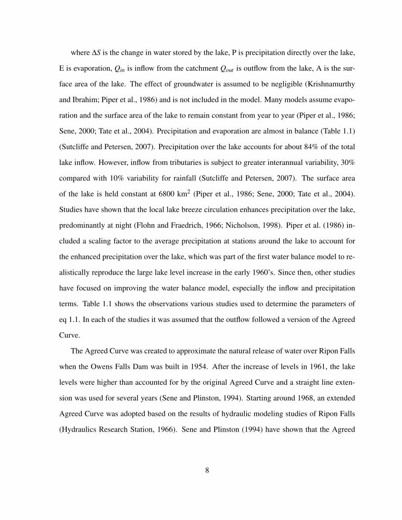
where ∆S is the change in water stored by the lake, P is precipitation directly over the lake,
E is evaporation, Qin is inflow from the catchment Qout is outflow from the lake, A is the sur-
face area of the lake. The effect of groundwater is assumed to be negligible (Krishnamurthy
and Ibrahim; Piper et al., 1986) and is not included in the model. Many models assume evapo-
ration and the surface area of the lake to remain constant from year to year (Piper et al., 1986;
Sene, 2000; Tate et al., 2004). Precipitation and evaporation are almost in balance (Table 1.1)
(Sutcliffe and Petersen, 2007). Precipitation over the lake accounts for about 84% of the total
lake inflow. However, inflow from tributaries is subject to greater interannual variability, 30%
compared with 10% variability for rainfall (Sutcliffe and Petersen, 2007). The surface area
of the lake is held constant at 6800 km2 (Piper et al., 1986; Sene, 2000; Tate et al., 2004).
Studies have shown that the local lake breeze circulation enhances precipitation over the lake,
predominantly at night (Flohn and Fraedrich, 1966; Nicholson, 1998). Piper et al. (1986) in-
cluded a scaling factor to the average precipitation at stations around the lake to account for
the enhanced precipitation over the lake, which was part of the first water balance model to re-
alistically reproduce the large lake level increase in the early 1960’s. Since then, other studies
have focused on improving the water balance model, especially the inflow and precipitation
terms. Table 1.1 shows the observations various studies used to determine the parameters of
eq 1.1. In each of the studies it was assumed that the outflow followed a version of the Agreed
Curve.
The Agreed Curve was created to approximate the natural release of water over Ripon Falls
when the Owens Falls Dam was built in 1954. After the increase of levels in 1961, the lake
levels were higher than accounted for by the original Agreed Curve and a straight line exten-
sion was used for several years (Sene and Plinston, 1994). Starting around 1968, an extended
Agreed Curve was adopted based on the results of hydraulic modeling studies of Ripon Falls
(Hydraulics Research Station, 1966). Sene and Plinston (1994) have shown that the Agreed
8
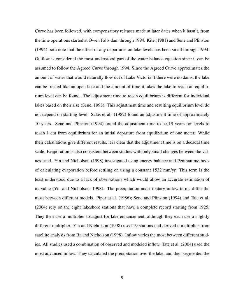
Curve has been followed, with compensatory releases made at later dates when it hasn’t, from
the time operations started at Owen Falls dam through 1994. Kite (1981) and Sene and Plinston
(1994) both note that the effect of any departures on lake levels has been small through 1994.
Outflow is considered the most understood part of the water balance equation since it can be
assumed to follow the Agreed Curve through 1994. Since the Agreed Curve approximates the
amount of water that would naturally flow out of Lake Victoria if there were no dams, the lake
can be treated like an open lake and the amount of time it takes the lake to reach an equilib-
rium level can be found. The adjustment time to reach equilibrium is different for individual
lakes based on their size (Sene, 1998). This adjustment time and resulting equilibrium level do
not depend on starting level. Salas et al. (1982) found an adjustment time of approximately
10 years. Sene and Plinston (1994) found the adjustment time to be 19 years for levels to
reach 1 cm from equilibrium for an initial departure from equilibrium of one meter. While
their calculations give different results, it is clear that the adjustment time is on a decadal time
scale. Evaporation is also consistent between studies with only small changes between the val-
ues used. Yin and Nicholson (1998) investigated using energy balance and Penman methods
of calculating evaporation before settling on using a constant 1532 mm/yr. This term is the
least understood due to a lack of observations which would allow an accurate estimation of
its value (Yin and Nicholson, 1998). The precipitation and tributary inflow terms differ the
most between different models. Piper et al. (1986); Sene and Plinston (1994) and Tate et al.
(2004) rely on the eight lakeshore stations that have a complete record starting from 1925.
They then use a multiplier to adjust for lake enhancement, although they each use a slightly
different multiplier. Yin and Nicholson (1998) used 19 stations and derived a multiplier from
satellite analysis from Ba and Nicholson (1998). Inflow varies the most between different stud-
ies. All studies used a combination of observed and modeled inflow. Tate et al. (2004) used the
most advanced inflow. They calculated the precipitation over the lake, and then segmented the
9
basin into five main sub-catchments. They then used a non-linear function, explained further
in section 3.5, to relate the inflow from each sub-catchment to the precipitation over the lake.
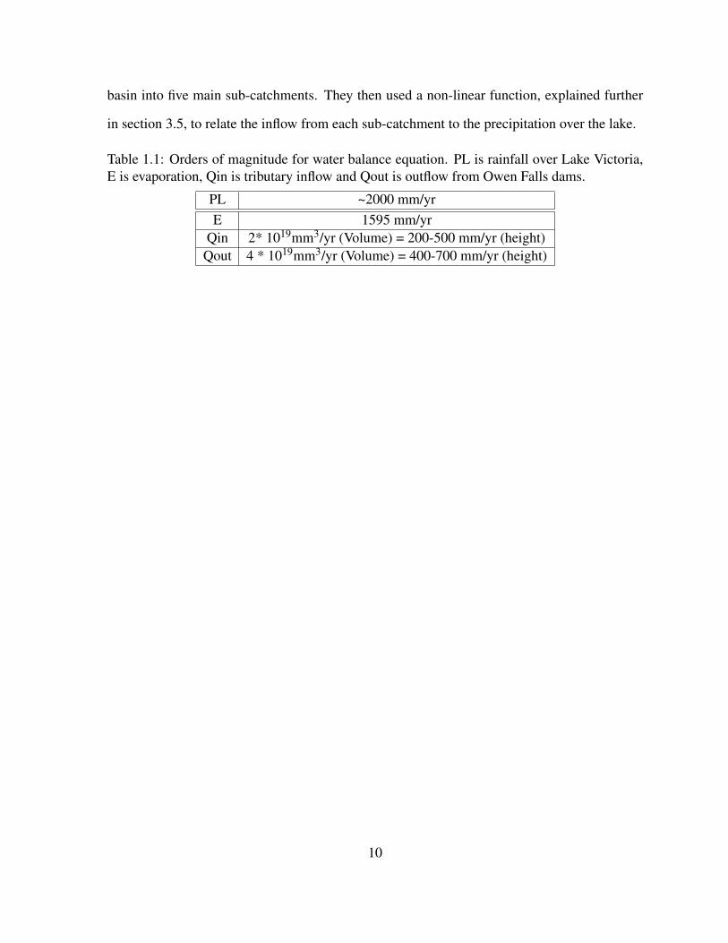
Table 1.1: Orders of magnitude for water balance equation. PL is rainfall over Lake Victoria,E is evaporation, Qin is tributary inflow and Qout is outflow from Owen Falls dams.
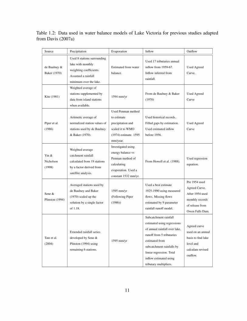
Table 1.2: Data used in water balance models of Lake Victoria for previous studies adaptedfrom Davis (2007a)
Source Precipitation Evaporation Inflow Outflow
de Baulney &
Baker (1970)
Used 8 stations surrounding
lake with monthly
weighting coefficients.
Assumed a rainfall
minimum over the lake.
Estimated from water
balance.
Used 17 tributaries annual
inflow from 1959-67.
Inflow inferred from
rainfall.
Used Agreed
Curve.
Kite (1981)
Weighted average of
stations supplemented by
data from island stations
when available.
1594 mm/yrFrom de Baulney & Baker
(1970)
Used Agreed
Curve
Piper et al.
(1986)
Aritmetic average of
normalized station values of
stations used by de Baulney
& Baker (1970).
Used Penman method
to estimate
precipitation and
scaled it to WMO
(1974) estimate. 1595
mm/year.
Used historical records.
Filled gaps by estimation.
Used estimated inflow
before 1956.
Used Agreed
Curve
Yin &
Nicholson
(1998)
Weighted average
catchment rainfall
calculated from 19 stations
by a factor derived from
satellite analysis.
Investigated using
energy balance vs
Penman method of
calculating
evaporation. Used a
constant 1532 mm/yr.
From Howell et al. (1988).Used regression
equation.
Sene &
Plinston (1994)
Averaged stations used by
de Baulney and Baker
(1970) scaled up the
solution by a single factor
of 1.18.
1595 mm/yr
(Following Piper
(1986))
Used a best estimate
1925-1990 using measured
flows. Missing flows
estimated by 9 parameter
rainfall runoff model.
Pre 1954 used
Agreed Curve.
After 1954 used
monthly records
of release from
Owen Falls Dam.
Tate et al.
(2004)
Extended rainfall series
developed by Sene &
Plinston (1994) using
remaining 6 stations.
1595 mm/yr
Subcatchment rainfall
estimated using regressions
of annual rainfall over lake,
runoff from 5 tributaries
estimated from
subcatchment rainfalls by
linear regression. Total
inflow estimated using
tributary multipliers.
Agreed curve
used on an annual
basis to find lake
level and
calculate revised
outflow.
11
1.2 History of Lake Victoria and Nile Basin
1.2.1 Egypt
Egypt, the most dependent nation on Nile waters, depends on the Nile for irrigation (Wa-
terbury, 2002). Egypt receives about 98 percent of its fresh water from the Nile, which satisfies
more than 95 percent of their water requirements (Tvedt, 2009). Egypt has entered many con-
tracts with other countries including the 1929 Agreement, the Owen Falls Dam agreements
with Britain on behalf of Uganda and the 1959 Agreement for full utilization of Nile Waters
with Sudan. The main goal of these agreements is to prevent any construction along the Nile
River which would modify the flow in any way which would be detrimental to Egypt. Water
from Lake Victoria minus evaporation losses in the Sudd region, contributes between 20% and
25% of the total Nile flow to Egypt (Howell and Allan, 1994; Garretson, 1967). While the
largest contribution comes from the Blue Nile, its contribution is less steady due to seasonal
and annual fluctuations in its tributaries.
1.2.2 Sudan
All major tributaries of the Nile, the White Nile, Blue Nile and Atbara join in Sudan to
form the main Nile. The economy of Sudan depends heavily on agriculture, most of which
is not farmed under irrigation from the Nile. The 1929 Nile River agreement did not define
water rights in quantitative terms, however the 1920 report of the Nile Projects Commission
suggested that Egypt should be guaranteed sufficient water to irrigate the maximum 5 million
feddans cultivated up to that time. Quantitative estimates were derived which gave Egypt
12
rights to 48 bcm and Sudan 4 bcm (Tvedt, 2003). The 1929 agreement stated that Sudan
could take water from the Nile and its tributaries from July 15 to December 31 each year
without limitations, enough to irrigate 38,500 feddans from January 1 to February 28, and
enough to irrigate 22,500 feddans from March 1 to July 15 (Tothill, 1948). When Sudan gained
independence in 1956, they declared that they did not have to take over the 1929 agreement
between Egypt and the British colonies and prepared to negotiate a new agreement (Howell
and Allan, 1994). The 1959 agreement with Egypt allowed Sudan 19.5 billion cubic meters
per year as measured at Aswan, or about 20.5 billion cubic meters in the area north of where
the White and Blue Niles merge in Khartoum (Waterbury, 2002).
1.2.3 Uganda
Uganda receives enough precipitation during the year that it does not depend on Lake Vic-
toria for irrigation. However, it does depend on the hydroelectric power plant at Owen’s Falls
for electricity. Owen’s Falls dam, renamed Nalubaale, and the newer Kiira dam control outflow
of Lake Victoria at Jinja, Uganda. A series of agreements between Egypt and Britain acting
on behalf of Uganda lead to the construction of Owen Falls dam. The agreement stated that
the Uganda Electricity Board could take any action in regard to the dam only after consultation
and agreement with the Egyptian government. The agreements dated between 1949 and 1954
are considered binding upon Uganda as long as Uganda uses the power supplied by the dam,
there are no new agreements and neither country renounces this agreement (Howell and Allan,
1994).
13
1.2.4 Tanzania
The government of Tanzania sent diplomatic letters to the governments of Britain, Egypt
and the Sudan on July 4th, 1962 outlining the policy of Tanzania on the use of Nile waters. In
these letters, the Tanzanian government stated that since the 1929 agreement applied to territo-
ries under British administration, the treaty lapsed when Tanzania became independent. This
became known as the Nyerere Doctrine (Howell and Allan, 1994). On November 21, 1963,
Egypt replied that “pending further agreement, the 1929 Nile Waters Agreement...remains valid
and applicable” (Seaton and Maliti, 1974).
1.2.5 Kenya
Even though six major tributaries of Lake Victoria flow through Kenya, two thirds of the
country is classified as semi-arid or arid (Howell and Allan, 1994). Kenya contributes 8.4 km3
per year of water to Lake Victoria (Tvedt, 2009). Kenya adopted a position similar to the
Nyerere Doctrine which indicates that the 1929 agreement ceased to apply to Kenya starting
December 12th, 1965.
1.3 Contribution of Lake Victoria to Upper Nile River
Since 1959, the Nalubaale Dam (originally called Owen Falls Dam) at Jinja, Uganda has
effectively turned Lake Victoria into a reservoir. The agreement since the dam was built is the
Agreed Curve that mimics the natural variability of the flow that went over Ripon Falls, the
natural rock weir submerged during the dam construction (Kull, 2006(a). This ranges between
300 and 1700 cubic meters per second depending on the level of the lake. While Nalubaale
dam was originally designed to provide 150 MW of energy when it was completed in 1954, it
14
has since been refurbished to provide 180 MW. Construction of Kiira dam was started in 1993
with plans for five hydroelectric turbine generators, which would each provide 40 megawatts.
The Bujagali dam, 250 MW is expected to be commissioned in 2011 further upstream, while
the Murchison Falls dam in Uganda and several other hydroelectric plants in Sudan are in the
planning phase. The flow of the White Nile, and hence the productivity of these dams are
primarily determined by the level of Lake Victoria.
1.4 Climatology & variability of the climate of Eastern Africa
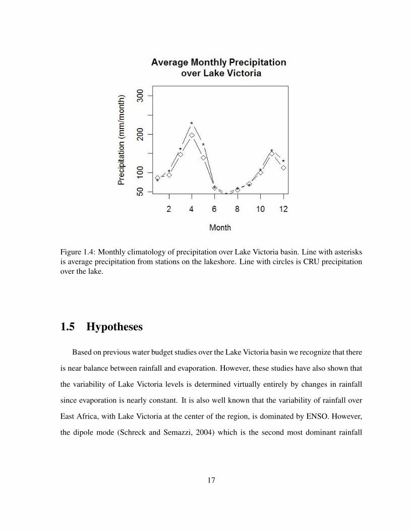
The general climate over Lake Victoria basin is characterized by a bimodal regime, the long
rains of March-May and the short rains of October-December. The October-December season
contributes disproportionately to the interannual variability of rainfall even though there is
more precipitation during the March-May season (Fig. 1.4). The seasonal cycle of rainfall is
mainly controlled by the north-south migration of the Intertropical Convergence Zone (ITCZ)
across the region, while the diurnal cycle is dominated by lake/land breeze circulations (Asnani,
2005). Earlier studies (Indeje et al., 2000; Asnani, 2005; Ogallo et al., 1988; Janowiak, 1988)
have established that the warm phase of ENSO causes greater precipitation over Eastern Africa.
Indeje et al. (2000) studied the evolution of ENSO modes in the seasonal rainfall patterns
over East Africa from 1961-1990 using empirical orthogonal function (EOF) and correlation
analysis to delineate a network of 136 stations over East Africa into eight homogeneous rainfall
regions to form rainfall indices. Other studies have noted that strong Indian Ocean zonal mode
events also cause an increase in precipitation in the area (Ummenhofer et al., 2009; Clark et al.,
2003).
Schreck and Semazzi (2004) performed an empirical orthogonal function (EOF) analysis
of gauge precipitation data and CPC Merged Analysis of Precipitation (CMAP) data which is
15
derived from rain gauge observations and satellite estimates. Their investigation covered the
October through November season from 1961-2001. Using Kendall’s (1980) criterion for dis-
tinctly separated EOFs, they determined that the first two EOF modes were significant. The
most dominant mode of variability based on CMAP data over eastern Africa corresponds to El
Niño-Southern Oscillation (ENSO) climate variability. The second eastern Africa EOF mode
was found to be a decadal trend with a loading characterized by a dipole pattern with positive
rainfall anomalies over the northern section of eastern Africa and negative rainfall anomalies
over the southern section which correlated significantly with a global warming index con-
structed by globally averaging surface temperature data from CRU archives. Their combined
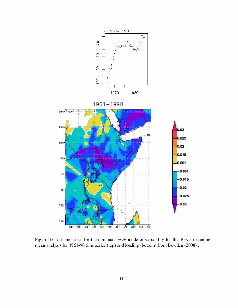
analysis of their time series and loading indicate that northern areas of eastern africa are getting
wetter, while southern areas are drying up during the time period 1961-2001.
16
Figure 1.4: Monthly climatology of precipitation over Lake Victoria basin. Line with asterisksis average precipitation from stations on the lakeshore. Line with circles is CRU precipitationover the lake.
1.5 Hypotheses
Based on previous water budget studies over the Lake Victoria basin we recognize that there
is near balance between rainfall and evaporation. However, these studies have also shown that
the variability of Lake Victoria levels is determined virtually entirely by changes in rainfall
since evaporation is nearly constant. It is also well known that the variability of rainfall over
East Africa, with Lake Victoria at the center of the region, is dominated by ENSO. However,
the dipole mode (Schreck and Semazzi, 2004) which is the second most dominant rainfall
17
climate mode also accounts for significant variability across the region with the Lake Victoria
Basin becoming more dry from 1961-1990. The hydrologic adjustment time described by Sene
(1998) and Sene and Plinston (1994) is also on a decadal scale.
Based on this knowledge, we hypothesize that ENSO dominates the variability of Lake
Victoria levels. We further hypothesize that the dipole mode and effects of the hydrologic
adjustment time of the lake also play significant roles but we are uncertain which of these two
is more significant. The relationship between the ENSO and dipole mode with Lake Victoria
levels is nonlinear and a key objective in this study is to estimate the relative contributions of
these modes in modulating Lake Victoria levels to test our hypothesis.
18
Chapter 2
Data
2.1 Lake Victoria Level Combined Data Set
The lake level data is based on a data set of lake level observations from January 1949 to
May 1998 at a gauge at the main river outlet in Jinja, Uganda obtained from an archive at the
Ministry of Water Resources in Uganda (Davis, 2007b). This data set was extended through
November 2007 using TOPEX/POSEIDON and Jason-1 altimetry satellite data (USDA, 2007).
Since the heights obtained by satellite altimetry are an average of all topography within the
instrument footprint further averaged in the direction of the satellite motion, these values differ
from traditional gauge measurements which are at specific points. Therefore, the TOPEX/
POSEIDON and Jason-1 altimetry data was supplied as a lake height variation with respect to
TOPEX/POSEIDON 10 year mean level. The climatological mean was found by subtracting
the satellite data from the observations for the time period the two data sets had in common
to determine the difference between the two. From this a mean was chosen and added to the
satellite anomalies. The mean was adjusted until bias and error were reduced to -4 * 10-4and
0.0585 respectively (Davis, 2007b). The remaining satellite altimetry time series was then
19
added to the resulting mean, creating a combined data set for January 1949 to November 2010.
The lake levels at the end of each year from this data set can be seen in figure 1.3.
2.2 Lake Victoria rain gauge precipitation
de Baulny and Baker (1970) originally used eight rain gauge stations (Jinja, Entebbe,
Kalangala, Bukoba, Kagondo, Mwanza, Musoma and Kisumu) around the shore of Lake Vic-
toria to determine precipitation over the lake for use in modeling the lake levels. The eight
stations were chosen since they were found to be the only lake shore stations to have good
quality records over long durations. Piper et al. (1986) and Sene and Plinston (1994) followed
de Baulny and Baker (1970) in using the eight stations while using a water balance model to
model Lake Victoria levels. All eight stations have records that date back to 1925, however we
were only able to obtain data from 1961-19990. Tate et al. (2004) extended the rainfall series of
Sene and Plinston (1994) omitting rainfall from Kalangala and Kagondo due to a lack of data
in recent years. In this study, we follow Tate et al. (2004) in using precipitation from Jinja,
Entebbe, Bukoba, Mwanza, Musoma and Kisumu to estimate precipitation over Lake Victoria.
The location of the six stations relative to Lake Victoria is shown in figure 2.1. For the EOF
analysis, we used a dataset of monthly precipitation for 136 stations unevenly distributed over
Uganda, Kenya and Tanzania from 1961-90. The six stations used to calculate precipitation
over the lake were included in this dataset.
20
Jinja
Mwanza
Musoma
Bukoba
Kisumu
Entebbe
Figure 2.1: Stations used in water balance model.
2.3 Climate Research Unit (CRU) TS 3.0 Precipitation
We used the Climate Research Unit’s CRU TS 3.0 to study the use of the water balance
model with data other than the stations mentioned in Section 3.5, since station data is not al-
ways easily available. CRU TS 3.0 is a monthly climatology of station data from 1901 through
2005. Station data is collected from several sources to form a global data set, which is checked
and corrected using an automated process. After the correction, a reference series is found for
a chosen baseline period (1961-1990). Anomalies are then found from the baseline climato-
logical normal and interpolated using angular distance-weighted (ADW) interpolation to a 0.5
degree grid (New et al., 2000). The gridded anomalies are then added back to the baseline
21
period climatological normal to create the grids (Mitchell and Jones, 2005). Unlike previ-
ous versions of CRU, no homogenization is performed in CRU TS 3.0. Homogenization is a
procedure used to correct any inhomogeneities in a station record caused by changes in instru-
mentation, station moves, or a change in observing practices (Peterson et al., 1998). For this
study we use data from 1950-2005 because Lake Victoria levels are available starting in 1949.
2.4 NASA Finite Volume Global Climate Model (FvGCM)
We used data from the NASA Finite Volume global climate model (FvGCM) used in the
PRUDENCE international model inter-comparison project, where two sets of FvGCM model
runs for present-day and A2 scenario runs were conducted. The model has a mass-conserving
finite-volume dynamical core (Lin et al., 2004). It was run at 1° latitude x 1.25° longitude reso-
lution with 18 vertical hybrid coordinate levels using the NCAR CCM3 physics package (Kiehl
et al., 1996). The model was forced by observed SSTs, sea ice distribution and greenhouse gas
concentrations for the reference run (1961-1990) and a spatially varying monthly SST per-
turbation calculated from corresponding experiments with the Hadley Center coupled model
HADCM3 was added to the reference run values to obtain SSTs for the A2 scenario experiment
(2071-2100)(Coppola and Giorgi, 2005). This is important because the model variability in the
coupled experiments does not have perfect SST boundary conditions and can be an additional
source of error.
2.5 RegCM3
We use model precipitation from the RegCM3 model runs performed by Bowden (2008).
He adopted the regional climate modeling approach to downscale present (RF, 1961-1990) and
22
a future (IPCC-A2, 2071-2100) climates generated by the NASA Finite Volume General Cir-
culation Model (FvGCM) using the ICTP REGional Climate Model version 3 (RegCM3). The
model is an updated version of the model previously customized for East Africa by Sun et al.
(1999) and Anyah and Semazzi (2007). The RegCM3 model is coupled to a one-dimensional
lake model which permits realistic vertical diffusion of heat energy. The domain has resolution
of 40km with lateral and boundary conditions for RF and A2 constructed from the correspond-
ing FvGCM runs. This domain is approximately 16.3° S to 20.7° N and 21.3° E to 55.1° E and
encompasses the countries of Burundi, Ethiopia, Kenya, Rwanda, Somalia, Sudan, Tanzania
and Uganda.
2.6 IPCC Ensemble
In order to examine the potential effect of climate change on Lake Victoria levels, we
used precipitation from an ensemble of IPCC AR4 models. The global climate model sim-
ulations were obtained from Coupled Model Inter-comparison Project (CMIP; http://www-
pcmdi.llnl.gov). The subset of models used had 20th century simulations and A2 simulations
run with comparable model physics with a resolution of 2.8 degrees or finer. This criteria pro-
vided us with 9 IPCC AR4 models out of the 23 models available, table 2.6 (Bowden, 2008).
Horizontal resolution for the IPCC AR4 models varies from 1.4 to 2.8 degrees. The finer
models were interpolated to the courser 2.8 degree resolution using a bi-linear interpolation to
create the IPCC ensemble. The ensemble has all of the 35 ensemble members for each GCM
included.
23
Table 2.1: Summary of selected IPCC AR4 models, their resolution and number of ensemblemembers used in the ensemble average for each model from Bowden (2008).
Short name CMIP3-ID Resolution # ensemble membersCanadian CGCM 2.8 x 2.8 5CCSM3 CCSM3 1.4 x 1.4 8ECHAM ECHAM/MPI-OM 1.9 x 1,9 4FRANCE CNRM-CGCM3 1.9 x 1.9 1
GFDL GFDL-CM2.0 2 x 2.5 4JAPAN MRI-CGCM.3.2 2.8 x 2.8 5PCM PCM 2.8 x 2.8 4
TOKYO MIROC3.2(medres) 2.8 x 2.8 3UK HADGEM1 1.3 x 1.9 2
2.7 Extended Reconstruction Sea Surface Temperature Ver-
sion 3 (ERSST.v3)
Sea surface temperature (SST) observations from the Advanced Very High Resolution Ra-
diometer (AVHRR) Pathfinder day and night satellite from 1985-2006 have been merged into
the ERSST.v3 dataset (Smith et al., 2008). Satellite data biases are normally associated with
aerosols and clouds, both of which cause a cold bias. The satellite SST bias is adjusted relative
to the merged ship and buoy SSTs before being incorporated into the dataset (Smith et al.,
2008).
24
Chapter 3
Method of Analysis
The primary method of investigation is a water balance model in combination with appli-
cation of EOF analysis of the regional Eastern Africa rain gauge rainfall. The water balance
model employs rainfall at six discrete locations around the lake to construct the Lake Vic-
toria levels. We adopt the EOF approach to isolate the contribution of individual significant
EOF mode and reconstruct the lake levels based on the water balance model. The results are
compared with the Lake Victoria levels constructed by using the total rainfall.
We compare the performance of the water balance model with observed Lake Victoria
levels and investigate the feasibility of the water balance model for the study. Since the water
balance model is based on stations, we first computed the dominant modes of variability based
on station data over Eastern Africa. Unfortunately the station data we obtained does not cover
precipitation more recent than 1990. We have used CRU data, after checking that it reproduces
salient features consistently, to model a longer time period.
25
3.1 Empirical Orthogonal Function (EOF) Analysis
Empirical orthogonal function analysis was performed on precipitation in Eastern Africa
in order to examine the effect of different modes of precipitation variability on rainfall over
eastern Africa and compare the modes derived from various data sets. Empirical Orthogonal
Function is a statistical tool used to explain the variance-covariance of geophysical data fields
through a few modes of variability. Two modes are spatially and temporally uncorrelated due
to the orthogonal nature of the EOF.
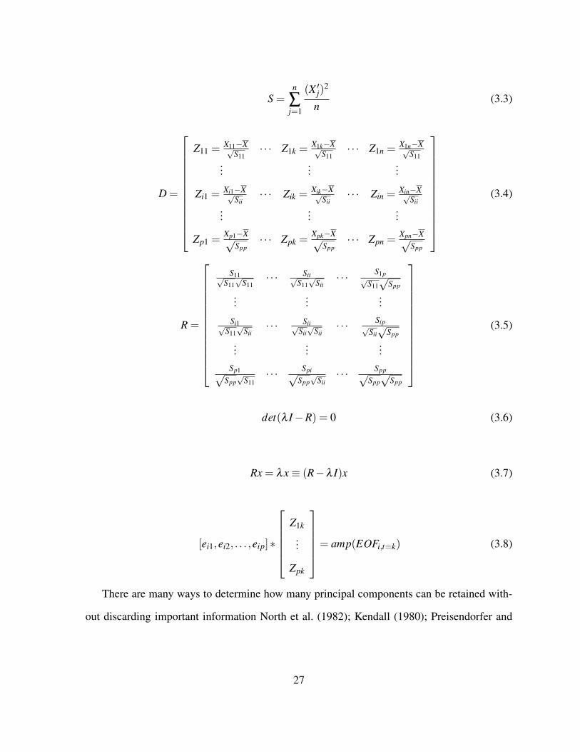
To calculate the EOFs the observational data is expressed in a n by p matrix where n is the
number of stations and p is the number of years, eqn. 3.1. Temporal anomalies, eq 3.2, are
found for the variable of interest for each station. The variance, eqn. 3.3, is also calculated to
standardize the data matrix, eqn. 3.4. The correlation matrix, eqn. 3.5, is then constructed in
order to form a non-dimensionalized version of the data such that the data has unit variance
(Wilks, 1995). We then generate eigenvalues by solving the characteristic equation determi-
nant, eqn. 3.6, for λ . The eigenvalues, λi correspond to the variance explained by each EOF
mode, EOFi. Once λ is known, the eigenvectors are found by solving eqn. 3.7 for x. The eigen-
vectors give the spatial pattern for each EOF mode. Finally, we construct the EOF time series
for each mode using eqn. 3.8, where ei is the eigenvector for EOFi and Zk is the standardized
data at time t.
X =
x11 x12 · · · x1p
x21 x22 · · · x2p
......
...
xn1 xn2 · · · xnp
(3.1)
X ′ = X−X (3.2)
26
S =n
∑j=1
(X ′j)2
n(3.3)
D =
Z11 =X11−X√
S11· · · Z1k =
X1k−X√S11
· · · Z1n =X1n−X√
S11...
......
Zi1 =Xi1−X√
Sii· · · Zik =
Xik−X√Sii
· · · Zin =Xin−X√
Sii...
......
Zp1 =Xp1−X√
Spp· · · Zpk =
Xpk−X√Spp
· · · Zpn =Xpn−X√
Spp
(3.4)
R =
S11√S11√
S11· · · Sii√
S11√
Sii· · · S1p√
S11√
Spp
......
...
Si1√S11√
Sii· · · Sii√
Sii√
Sii· · · Sip√
Sii√
Spp
......
...Sp1√
Spp√
S11· · · Spi√
Spp√
Sii· · · Spp√
Spp√
Spp
(3.5)
det(λ I−R) = 0 (3.6)
Rx = λx≡ (R−λ I)x (3.7)
[ei1,ei2, . . . ,eip]∗
Z1k
...
Zpk
= amp(EOFi,t=k) (3.8)
There are many ways to determine how many principal components can be retained with-
out discarding important information North et al. (1982); Kendall (1980); Preisendorfer and
27
Barnett (1977). We test for significance of the modes using Kendall’s criterion for distinctly
separated EOFs, for sample size N, that sampling error δλ = λ (2/N)1/2, associated with a
given eigenvalue λ , must be smaller than its spacing from the neighboring eigenvalue. We then
relate the spatial patterns to known physical properties, such as ENSO and IOZM.
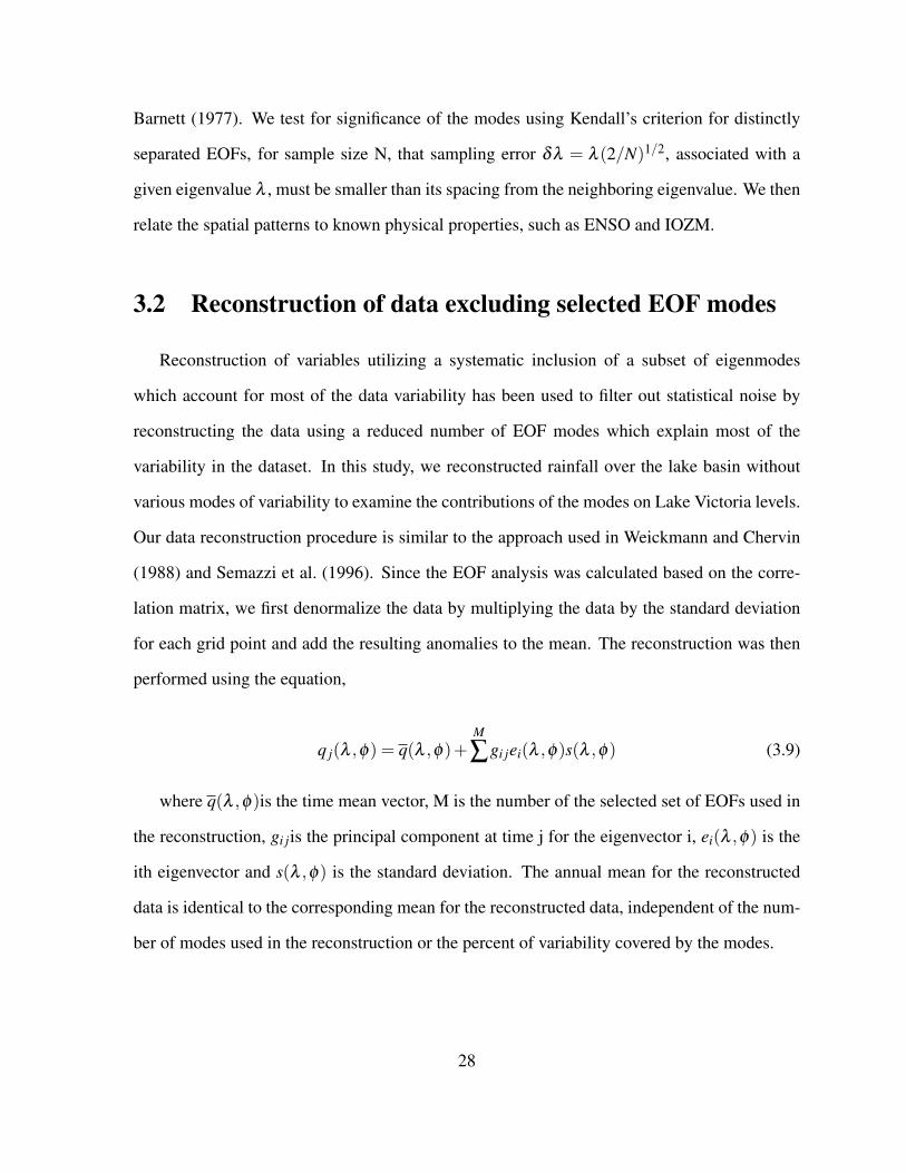
3.2 Reconstruction of data excluding selected EOF modes
Reconstruction of variables utilizing a systematic inclusion of a subset of eigenmodes
which account for most of the data variability has been used to filter out statistical noise by
reconstructing the data using a reduced number of EOF modes which explain most of the
variability in the dataset. In this study, we reconstructed rainfall over the lake basin without
various modes of variability to examine the contributions of the modes on Lake Victoria levels.
Our data reconstruction procedure is similar to the approach used in Weickmann and Chervin
(1988) and Semazzi et al. (1996). Since the EOF analysis was calculated based on the corre-
lation matrix, we first denormalize the data by multiplying the data by the standard deviation
for each grid point and add the resulting anomalies to the mean. The reconstruction was then
performed using the equation,
q j(λ ,φ) = q(λ ,φ)+M
∑gi jei(λ ,φ)s(λ ,φ) (3.9)
where q(λ ,φ)is the time mean vector, M is the number of the selected set of EOFs used in
the reconstruction, gi jis the principal component at time j for the eigenvector i, ei(λ ,φ) is the
ith eigenvector and s(λ ,φ) is the standard deviation. The annual mean for the reconstructed
data is identical to the corresponding mean for the reconstructed data, independent of the num-
ber of modes used in the reconstruction or the percent of variability covered by the modes.
28
3.3 Reconstructed data demonstration
We demonstrate how the method described in Section 3.2 works in practice using only 3
stations. The original standardized data can be reconstructed by multiplying the EOF time
series and the eigenvectors. We will use an example proof to demonstrate the EOF and its
reconstruction. The proof is based on standardized data for three stations for four years. There
can be p number of stations for t years.
Table 3.1: Standardized precipitation for three stations over four years.
Linear correlation is a well-known statistical tool within climatology. Our study uses linear
correlations to determine relationships between EOF mode time series from different seasons
and data sets. Grid point correlations between SST anomaly fields and EOF mode time series
were also calculated to help determine their sources of variability.
3.5 Water Balance Model
Tate et al. (2004) and others (Sene and Plinston, 1994; Sene, 2000), developed a water bal-
ance model to estimate the level of Lake Victoria at the end of a given year (Ln) by calculating
the change in lake level during the year (∆L) and adding it to the projected level for the previous
year (Ln−1(estimated)).
The change in lake level is calculated as:
∆Ln =
[P−E +
Qin−Qout
A
]n
(3.10)
Where P and E are precipitation and evaporation over the lake, respectively, Qinis inflow
to the lake from tributaries, Qout is outflow from the dams at Jinja, and A is the surface area
of Lake Victoria. Evaporation is assumed constant at 1595 mm/year. Precipitation over the
lake, the dominant source of water for Lake Victoria, is assumed to be a linear function of the
average annual rain gauge precipitation at eight stations (Jinja, Entebbe, Kisumu, Musoma,
Bukoba, Mwanza, Kalangala and Kagondo) along the perimeter of the lake. When gridded
precipitation datasets are used (CRU, FvGCM, RegCM3, IPCC ensemble), the precipitation is
first interpolated to the six station using WENO interpolation, and then the interpolated station
precipitation values are used in place of station gauge precipitation. The inflow, Qin, from five
31
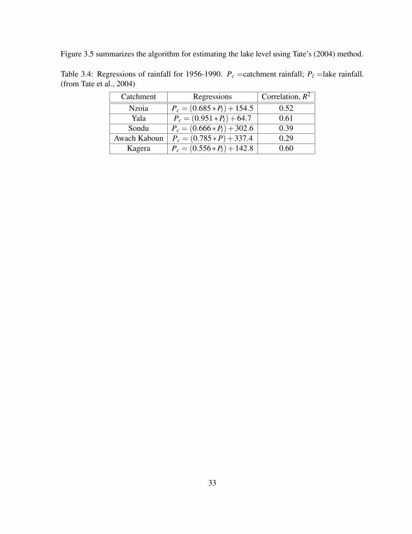
tributaries (Nzoia, Yala, Sondu, Awach Kaboun, and Kagera) is a non-linear function with P
as the input. Subcatchment rainfalls, Pc, for each of the five tributaries were estimated using
regressions of annual total data for the period 1965-1990 (table 3.4). The runoff coefficient for
each catchment is then estimated from the subcatchment rainfall by linear regression derived
by Sutcliffe and Parks (1999) as:
rc = 0.0002Pc−0.1386 (3.11)
The runoff from each subcatchment to Lake Victoria is then estimated by multiplying each
subcatchment’s rainfall by the runoff coefficient and the subcatchment area. The total inflow to
Lake Victoria is estimated as the runoff of Nzoia, Yala, Sondu and Awach Kaboun scaled up by
a factor of 2.7 on an annual basis, plus the flow of the Kagera increased by 10% to account for
the flow of the Ngono tributary, which joins it downstream of the gauging station (Tate et al.,
2004; Institute of Hydrology, 1985). The outflow, Qout , is calculated from the Agreed Curve
which has the form:
Qoutn = α(Ln−β )γ (3.12)
where α and γ are empirical coefficients, and β is a datum value, or reference point against
which measurements are made (Sene, 2000). Substituting (Eq. 3.12) into (Eqn 3.10) produces:
∆Ln =
[(P−E +
Qin
A
)n−(α(L(n−1)observed +∆Ln−β )γ
)/A]
(3.13)
where α= 70.332 (or 66.3); β= 8.058 (or 7.96); and γ= 2.00 (or 2.01) depending on the
equation used (Koren, 1995; Sene, 2000). Since ∆Ln appears as a term on the left hand side
and in the nonlinear term on the right hand side of (Eqn. 3.13), the equation must be solved
iteratively. This procedure is executed using two iterations setting ∆Ln= 0 on the first iteration.
32
Figure 3.5 summarizes the algorithm for estimating the lake level using Tate’s (2004) method.
Table 3.4: Regressions of rainfall for 1956-1990. Pc =catchment rainfall; Pl =lake rainfall.(from Tate et al., 2004)
Catchment Regressions Correlation, R2
Nzoia Pc = (0.685∗Pl)+154.5 0.52Yala Pc = (0.951∗Pl)+64.7 0.61
Sondu Pc = (0.666∗Pl)+302.6 0.39Awach Kaboun Pc = (0.785∗P)+337.4 0.29
Kagera Pc = (0.556∗Pl)+142.8 0.60
33
Figure 3.1: Water balance model algorithm for Lake Victoria used by Tate et al. (2004). Thedashed arrow is not followed in the modified algorithm used in this study.
34
3.5.1 Agreed Curve Outflow
There are four versions of the Agreed Curve. Koren (1995) created an agreed curve,
Qoutn = 70.332(Ln− 8.058)2 Sene (2000) developed a similar formula with slightly different
coefficients, Qoutn = 66.3(Ln− 7.96)2.01 by fitting a curve to observed levels and discharges
over a long period of time. According to Sutcliffe and Petersen (2007), the actual equation
used by the Directorate of Water Development is Qoutn = 132.9238(Ln− 8.486)1.686. These
three formulations produce similar results. Figure 3.2 shows the Agreed Curve for discharge
from the Owens Falls Dams based on Lake Victoria’s level. Power Planning Associates Ltd
(2007) have suggested a constant Agreed Curve, or Agreed Curve by steps, where the release
would be a constant 687 m3/s during low hydrology scenarios and 1247 m3/s during high
hydrology scenarios. The low hydrology scenario is defined as annual variations around an
average net basin supply (NBS) of 660 m3/s, which is consistent with the years 1900-1959.
The high hydrology scenario is defined as the NBS averaging more than 1000 m3/s, which is
consistent with the years 1960-1999. Annual NBS for 1900-2005 is shown in figure 3.3. They
then suggest that in an optimized operation situation, the lake would not fall to the minimum
acceptable value if the release had been reduced to a constant intermediate value, approxi-
mately 900 m3/s, as soon as the lake level decreases below approximately 1135 m above sea
level. The curve developed by Sene (2000) will be used in this study.
35
Figure 3.2: The Agreed Curve for outflow from Lake Victoria based on lake levels.
Figure 3.3: Yearly net basin supply (blue) and outflow (red) for Lake Victoria (1900-2005)from Power Planning Associates (2007).
36
3.6 Bias Removal
We used a simple normalization technique to adjust the model systematic bias for FvGCM,
RegCM3 and the IPCC ensemble. This is done using the equation:
(yi− yavg) =
√Six√Siy
+ xavg (3.14)
where y is the model precipitation; yavg is the mean model precipitation;√
Six is the ob-
served standard deviation;√
Siy is the model standard deviation; and xavg is the mean observed
precipitation. For observed values we use CRU precipitation. The bias correction average and
standard deviation values are calculated for each month for all grid points i. The normalization
technique preserved the variance but adjusts the values to the observed mean. We apply this
method to the A2 scenario runs by removing the model mean for the reference period (yavg)
and adding the observed reference mean (xavg). The difference between the observed mean
and the observed A2 precipitation values will still have the mean climate change signal while
preserving the variance of the A2 simulations.
37
Chapter 4
Results
4.1 Lake Victoria Levels
We use a water balance model developed by Tate et al. (2004) to investigate the role
of the following factors in modulating the Lake Victoria levels: climate variability factors:
the regional response to ENSO and IOZM and other interannual and decadal climate modes,
anthropogenic causes: distorted outflow from dams and non-linear feedbacks due to changes in
land cover, and non-climate geophysical changes: the time necessary for lake levels to adjust
to equilibrium and changes in level due to accumulation of bottom sedimentation.
We first show that we can reproduce Lake Victoria levels using precipitation from six of the
original eight stations in the water balance model. Unlike Tate et al. (2004) we start the model
in 1960 so that we can use precipitation from stations in the East African region to obtain and
analyze the significant modes of variability in Section 4.3 for the same years. We then show
that CRU TS 3.0 precipitation in the model gives similar levels for the same time period. This
is done in order to obtain confidence so we can use the longer and more current 1950-2005
CRU TS 3.1 data to investigate the role of climate factors on lake levels over the longer time
38
period.
Lake Victoria levels calculated using the water balance model are shown as a red line in
figure 4.1. Our modeled levels do not capture the sudden increase in levels from 1961-64 as
well as the levels modeled by Tate et al. (2004) (Fig. 4.2). This is most likely because the
water balance model run by Tate et al. (2004) was initialized earlier than ours. Their model
run predicts higher than actual levels, starting approximately twenty years before the jump in
lake levels. These higher modeled levels give their lake levels a “boost” when it gets to the
early 1960’s, where the model had already accumulated extra water in the lake that then was
included in the 1961-64 levels. Our model starts before the jump and does not over predict lake
levels before 1961; therefore it does not have this extra water to use towards the higher levels
in 1963-64.
After the jump in levels, our model run does a good job of capturing the lake level, while the
model run by Tate et al. (2004) under predicts lake levels by small amounts in the 1970’s and
1980’s followed by predicting higher than actual lake levels in the mid to late 1990’s. When
CRU precipitation is used in the model (Fig.4.3), the first two years of the 1961-64 jump are
captured, while the modeled lake levels are a little low for 1963 and 1964. The model does
well until the 1980’s when it under-predicts lake levels by up to 0.5 meters in 1983 and then
predicts higher than actual levels in the late 1990’s through 2005, over-predicting by as much
as 0.73 m in 2005 which is most likely related to the over-release from Nalubaale and Kiira
dams found by Kull (2006(a) and expanded upon in Kull (2006(b). For the subsections 4.1.1
through 4.1.8, we will use the 1949-2005 CRU modeled levels as the true levels for comparison
purposes only in order to focus on the influence of the potential sources of lake level variability
being investigated and not model error.
39
Year
Leve
l (m
)
10.5
11.5
12.5
60 63 66 69 72 75 78 81 84 87 90
Figure 4.1: Station precipitation in water balance model. Blue line is actual lake levels fromsatellite altimetry, red line is modeled level.
Figure 4.2: Modeled vs observed Lake Victoria levels and outflows, 1925-2000. Top two linesare observed and modeled levels, lower two lines are observed and modeled outflow. FromTate et al. (2004), their figure 4.
40
Year
Leve
l (m
)
10.5
11.0
11.5
12.0
12.5
13.0
49 53 57 61 65 69 73 77 81 85 89 93 97 01 05
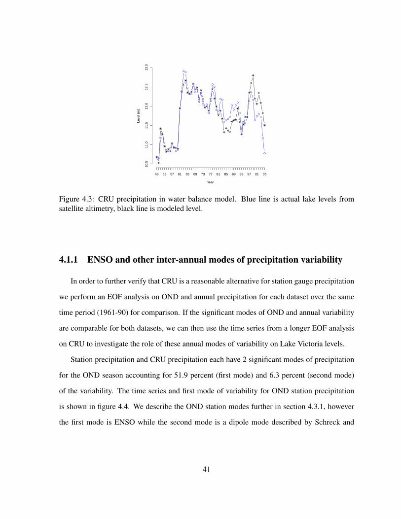
Figure 4.3: CRU precipitation in water balance model. Blue line is actual lake levels fromsatellite altimetry, black line is modeled level.
4.1.1 ENSO and other inter-annual modes of precipitation variability
In order to further verify that CRU is a reasonable alternative for station gauge precipitation
we perform an EOF analysis on OND and annual precipitation for each dataset over the same
time period (1961-90) for comparison. If the significant modes of OND and annual variability
are comparable for both datasets, we can then use the time series from a longer EOF analysis
on CRU to investigate the role of these annual modes of variability on Lake Victoria levels.
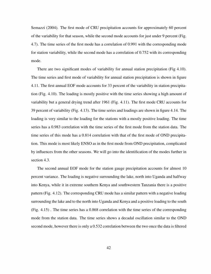
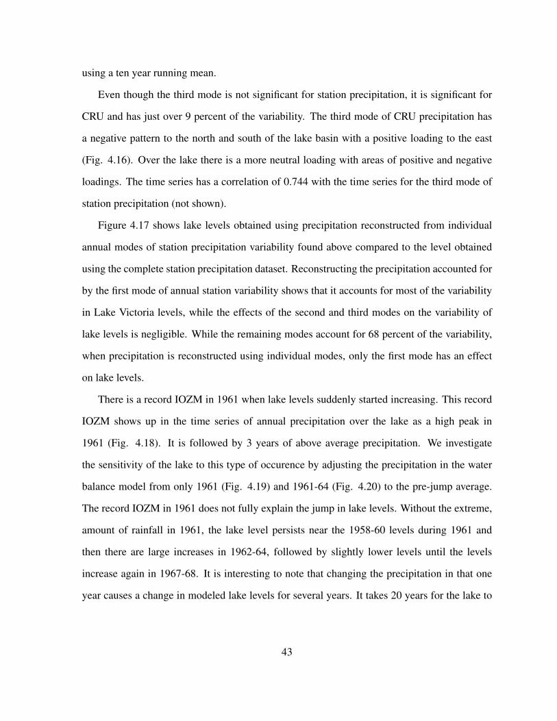
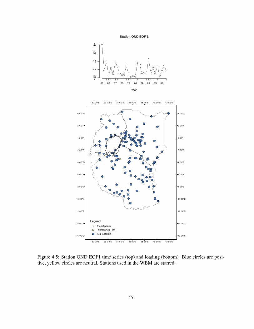
Station precipitation and CRU precipitation each have 2 significant modes of precipitation
for the OND season accounting for 51.9 percent (first mode) and 6.3 percent (second mode)
of the variability. The time series and first mode of variability for OND station precipitation
is shown in figure 4.4. We describe the OND station modes further in section 4.3.1, however
the first mode is ENSO while the second mode is a dipole mode described by Schreck and
41
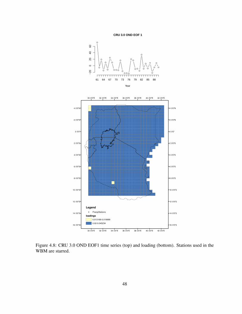
Semazzi (2004). The first mode of CRU precipitation accounts for approximately 60 percent
of the variability for that season, while the second mode accounts for just under 9 percent (Fig.
4.7). The time series of the first mode has a correlation of 0.991 with the corresponding mode
for station variability, while the second mode has a correlation of 0.752 with its corresponding
mode.
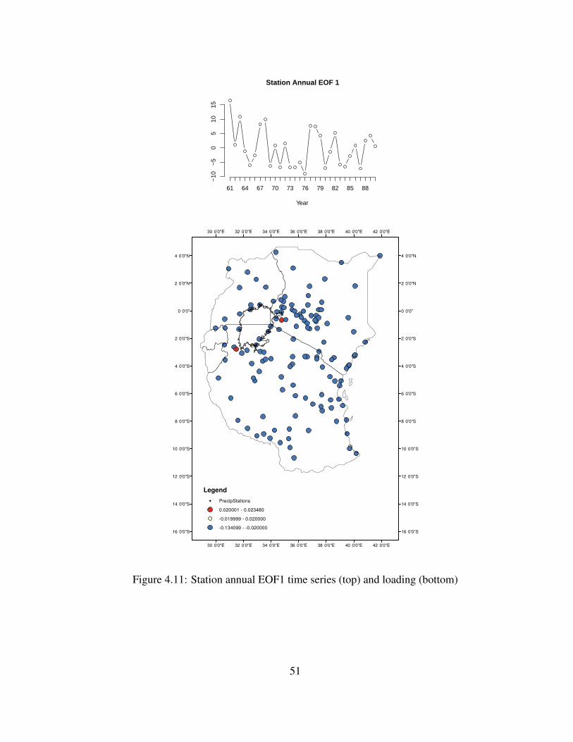
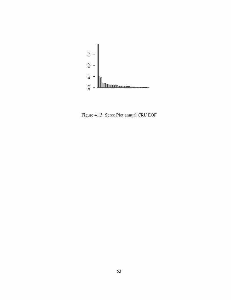
There are two significant modes of variability for annual station precipitation (Fig 4.10).
The time series and first mode of variability for annual station precipitation is shown in figure
4.11. The first annual EOF mode accounts for 33 percent of the variability in station precipita-
tion (Fig. 4.10). The loading is mostly positive with the time series showing a high amount of
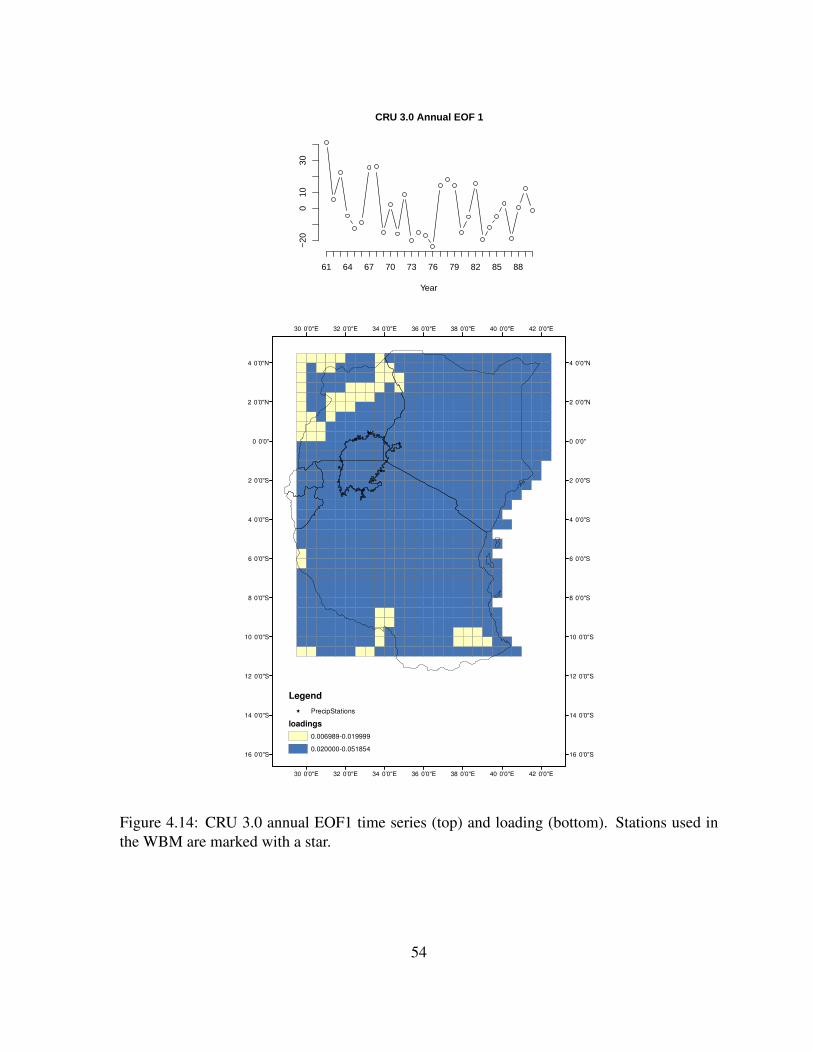
variability but a general drying trend after 1961 (Fig. 4.11). The first mode CRU accounts for
39 percent of variability (Fig. 4.13). The time series and loadings are shown in figure 4.14. The
loading is very similar to the loading for the stations with a mostly positive loading. The time
series has a 0.983 correlation with the time series of the first mode from the station data. The
time series of this mode has a 0.814 correlation with that of the first mode of OND precipita-
tion. This mode is most likely ENSO as in the first mode from OND precipitation, complicated
by influences from the other seasons. We will go into the identification of the modes further in
section 4.3.
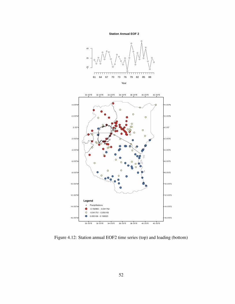
The second annual EOF mode for the station gauge precipitation accounts for almost 10
percent variance. The loading is negative surrounding the lake, north into Uganda and halfway
into Kenya, while it in extreme southern Kenya and southwestern Tanzania there is a positive
pattern (Fig. 4.12). The corresponding CRU mode has a similar pattern with a negative loading
surrounding the lake and to the north into Uganda and Kenya and a positive loading to the south
(Fig. 4.15) . The time series has a 0.868 correlation with the time series of the corresponding
mode from the station data. The time series shows a decadal oscillation similar to the OND
second mode, however there is only a 0.532 correlation between the two once the data is filtered
42
using a ten year running mean.
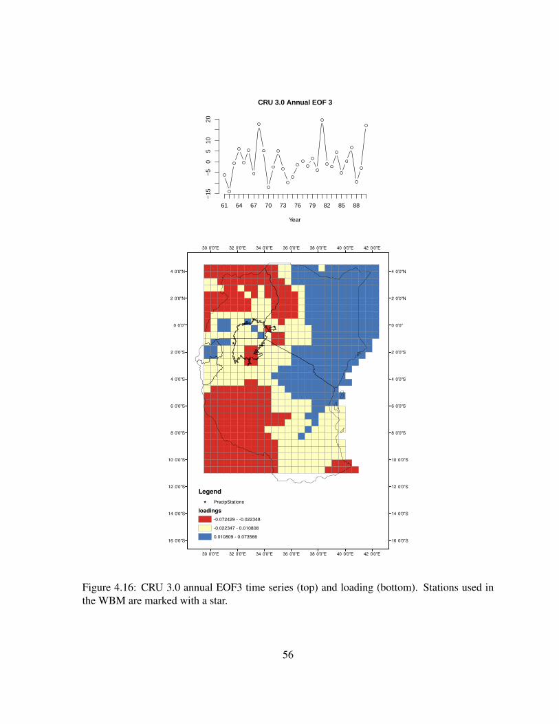
Even though the third mode is not significant for station precipitation, it is significant for
CRU and has just over 9 percent of the variability. The third mode of CRU precipitation has
a negative pattern to the north and south of the lake basin with a positive loading to the east
(Fig. 4.16). Over the lake there is a more neutral loading with areas of positive and negative
loadings. The time series has a correlation of 0.744 with the time series for the third mode of
station precipitation (not shown).
Figure 4.17 shows lake levels obtained using precipitation reconstructed from individual
annual modes of station precipitation variability found above compared to the level obtained
using the complete station precipitation dataset. Reconstructing the precipitation accounted for
by the first mode of annual station variability shows that it accounts for most of the variability
in Lake Victoria levels, while the effects of the second and third modes on the variability of
lake levels is negligible. While the remaining modes account for 68 percent of the variability,
when precipitation is reconstructed using individual modes, only the first mode has an effect
on lake levels.
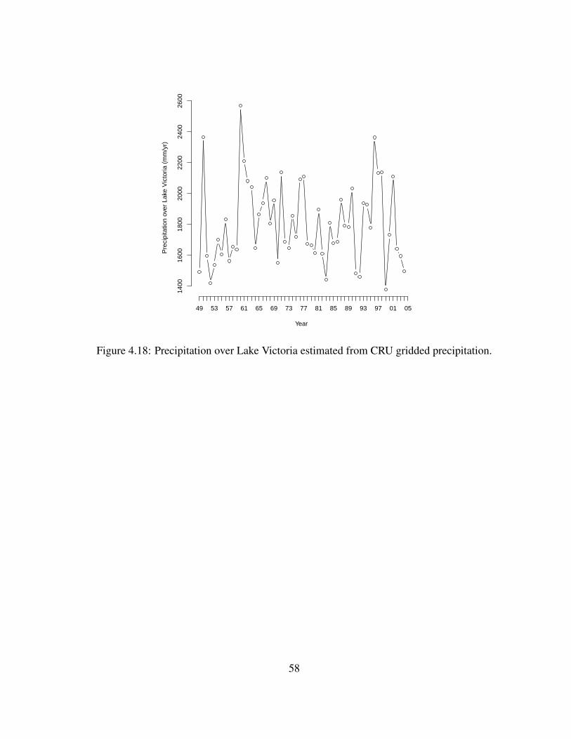
There is a record IOZM in 1961 when lake levels suddenly started increasing. This record
IOZM shows up in the time series of annual precipitation over the lake as a high peak in
1961 (Fig. 4.18). It is followed by 3 years of above average precipitation. We investigate
the sensitivity of the lake to this type of occurence by adjusting the precipitation in the water
balance model from only 1961 (Fig. 4.19) and 1961-64 (Fig. 4.20) to the pre-jump average.
The record IOZM in 1961 does not fully explain the jump in lake levels. Without the extreme,
amount of rainfall in 1961, the lake level persists near the 1958-60 levels during 1961 and
then there are large increases in 1962-64, followed by slightly lower levels until the levels
increase again in 1967-68. It is interesting to note that changing the precipitation in that one
year causes a change in modeled lake levels for several years. It takes 20 years for the lake to
43
return to within 0.01 meters of what the levels would have been without this change. This will
be explained further in section 4.1.3. When the extreme rainfall event in 1961-64 is removed in
the same manner, there is still a smaller, close to 1 meter, increase in levels from 1966-68. The
modeled lake levels for both scenarios do not reach the same height as the non-modified lake
for approximately 20 years in each scenario because the water balance model does not have
the higher levels from the years with modified precipitation to build upon. After the hydrologic
adjustment time, the precipitation from those years is not a factor in the lake levels.0.
00.
10.
20.
30.
40.
5
Station OND
Figure 4.4: Scree Plot OND Station EOF
44
Year
−10
010
2030
61 64 67 70 73 76 79 82 85 88
Station OND EOF 1
42°0’0"E
42°0’0"E
40°0’0"E
40°0’0"E
38°0’0"E
38°0’0"E
36°0’0"E
36°0’0"E
34°0’0"E
34°0’0"E
32°0’0"E
32°0’0"E
30°0’0"E
30°0’0"E
4°0’0"N 4°0’0"N
2°0’0"N 2°0’0"N
0°0’0" 0°0’0"
2°0’0"S 2°0’0"S
4°0’0"S 4°0’0"S
6°0’0"S 6°0’0"S
8°0’0"S 8°0’0"S
10°0’0"S 10°0’0"S
12°0’0"S 12°0’0"S
14°0’0"S 14°0’0"S
16°0’0"S 16°0’0"S
Legend
PrecipStations
-0.020332-0.01999
0.02-0.110032
Figure 4.5: Station OND EOF1 time series (top) and loading (bottom). Blue circles are posi-tive, yellow circles are neutral. Stations used in the WBM are starred.
45
Year
−4
02
46
861 64 67 70 73 76 79 82 85 88
Station OND EOF 2
42°0’0"E
42°0’0"E
40°0’0"E
40°0’0"E
38°0’0"E
38°0’0"E
36°0’0"E
36°0’0"E
34°0’0"E
34°0’0"E
32°0’0"E
32°0’0"E
30°0’0"E
30°0’0"E
4°0’0"N 4°0’0"N
2°0’0"N 2°0’0"N
0°0’0" 0°0’0"
2°0’0"S 2°0’0"S
4°0’0"S 4°0’0"S
6°0’0"S 6°0’0"S
8°0’0"S 8°0’0"S
10°0’0"S 10°0’0"S
12°0’0"S 12°0’0"S
14°0’0"S 14°0’0"S
16°0’0"S 16°0’0"S
Legend
PrecipStations
-0.163818 - -0.020000
-0.019999 - 0.020000
0.020001 - 0.202505
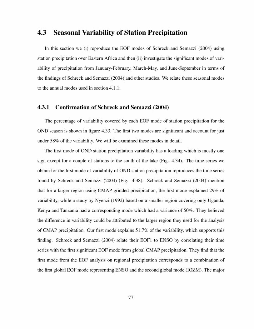
Figure 4.6: Station OND EOF2 time series (top) and loading (bottom). Blue circles are posi-tive, yellow circles are neutral, red circles are negative. Stations used in the WBM are starred.
46
0.0
0.2
0.4
0.6
Figure 4.7: Scree Plot OND CRU 3.0 EOF
47
Year
−20
020
4060
61 64 67 70 73 76 79 82 85 88
CRU 3.0 OND EOF 1
42°0’0"E
42°0’0"E
40°0’0"E
40°0’0"E
38°0’0"E
38°0’0"E
36°0’0"E
36°0’0"E
34°0’0"E
34°0’0"E
32°0’0"E
32°0’0"E
30°0’0"E
30°0’0"E
4°0’0"N 4°0’0"N
2°0’0"N 2°0’0"N
0°0’0" 0°0’0"
2°0’0"S 2°0’0"S
4°0’0"S 4°0’0"S
6°0’0"S 6°0’0"S
8°0’0"S 8°0’0"S
10°0’0"S 10°0’0"S
12°0’0"S 12°0’0"S
14°0’0"S 14°0’0"S
16°0’0"S 16°0’0"S
Legend
PrecipStations
loadings
0.013168-0.019999
0.02-0.045234
Figure 4.8: CRU 3.0 OND EOF1 time series (top) and loading (bottom). Stations used in theWBM are starred.
48
Year
−15
−5
05
1015
61 64 67 70 73 76 79 82 85 88
CRU 3.0 OND EOF 2
42°0’0"E
42°0’0"E
40°0’0"E
40°0’0"E
38°0’0"E
38°0’0"E
36°0’0"E
36°0’0"E
34°0’0"E
34°0’0"E
32°0’0"E
32°0’0"E
30°0’0"E
30°0’0"E
4°0’0"N 4°0’0"N
2°0’0"N 2°0’0"N
0°0’0" 0°0’0"
2°0’0"S 2°0’0"S
4°0’0"S 4°0’0"S
6°0’0"S 6°0’0"S
8°0’0"S 8°0’0"S
10°0’0"S 10°0’0"S
12°0’0"S 12°0’0"S
14°0’0"S 14°0’0"S
16°0’0"S 16°0’0"S
Legend
PrecipStations
loadings
-0.065254 - -0.021110
-0.021109 - 0.021943
0.021944 - 0.086587
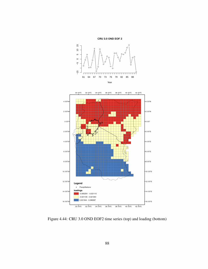
Figure 4.9: CRU 3.0 OND EOF2 time series (top) and loading (bottom)
49
0.00
0.10
0.20
0.30
Station Annual
Figure 4.10: Scree Plot annual Station EOF
50
Year
−10
−5
05
1015
61 64 67 70 73 76 79 82 85 88
Station Annual EOF 1
42°0’0"E
42°0’0"E
40°0’0"E
40°0’0"E
38°0’0"E
38°0’0"E
36°0’0"E
36°0’0"E
34°0’0"E
34°0’0"E
32°0’0"E
32°0’0"E
30°0’0"E
30°0’0"E
4°0’0"N 4°0’0"N
2°0’0"N 2°0’0"N
0°0’0" 0°0’0"
2°0’0"S 2°0’0"S
4°0’0"S 4°0’0"S
6°0’0"S 6°0’0"S
8°0’0"S 8°0’0"S
10°0’0"S 10°0’0"S
12°0’0"S 12°0’0"S
14°0’0"S 14°0’0"S
16°0’0"S 16°0’0"S
Legend
PrecipStations
0.020001 - 0.023480
-0.019999 - 0.020000
-0.134099 - -0.020000
Figure 4.11: Station annual EOF1 time series (top) and loading (bottom)
51
Year
−5
05
61 64 67 70 73 76 79 82 85 88
Station Annual EOF 2
42°0’0"E
42°0’0"E
40°0’0"E
40°0’0"E
38°0’0"E
38°0’0"E
36°0’0"E
36°0’0"E
34°0’0"E
34°0’0"E
32°0’0"E
32°0’0"E
30°0’0"E
30°0’0"E
4°0’0"N 4°0’0"N
2°0’0"N 2°0’0"N
0°0’0" 0°0’0"
2°0’0"S 2°0’0"S
4°0’0"S 4°0’0"S
6°0’0"S 6°0’0"S
8°0’0"S 8°0’0"S
10°0’0"S 10°0’0"S
12°0’0"S 12°0’0"S
14°0’0"S 14°0’0"S
16°0’0"S 16°0’0"S
Legend
PrecipStations
-0.192965 - -0.041752
-0.041751 - 0.055105
0.055106 - 0.156523
Figure 4.12: Station annual EOF2 time series (top) and loading (bottom)
52
0.0
0.1
0.2
0.3
Figure 4.13: Scree Plot annual CRU EOF
53
Year
−20
010
30
61 64 67 70 73 76 79 82 85 88
CRU 3.0 Annual EOF 1
42°0’0"E
42°0’0"E
40°0’0"E
40°0’0"E
38°0’0"E
38°0’0"E
36°0’0"E
36°0’0"E
34°0’0"E
34°0’0"E
32°0’0"E
32°0’0"E
30°0’0"E
30°0’0"E
4°0’0"N 4°0’0"N
2°0’0"N 2°0’0"N
0°0’0" 0°0’0"
2°0’0"S 2°0’0"S
4°0’0"S 4°0’0"S
6°0’0"S 6°0’0"S
8°0’0"S 8°0’0"S
10°0’0"S 10°0’0"S
12°0’0"S 12°0’0"S
14°0’0"S 14°0’0"S
16°0’0"S 16°0’0"S
Legend
PrecipStations
loadings
0.006989-0.019999
0.020000-0.051854
Figure 4.14: CRU 3.0 annual EOF1 time series (top) and loading (bottom). Stations used inthe WBM are marked with a star.
54
Year
−10
010
2061 64 67 70 73 76 79 82 85 88
CRU 3.0 Annual EOF 2
42°0’0"E
42°0’0"E
40°0’0"E
40°0’0"E
38°0’0"E
38°0’0"E
36°0’0"E
36°0’0"E
34°0’0"E
34°0’0"E
32°0’0"E
32°0’0"E
30°0’0"E
30°0’0"E
4°0’0"N 4°0’0"N
2°0’0"N 2°0’0"N
0°0’0" 0°0’0"
2°0’0"S 2°0’0"S
4°0’0"S 4°0’0"S
6°0’0"S 6°0’0"S
8°0’0"S 8°0’0"S
10°0’0"S 10°0’0"S
12°0’0"S 12°0’0"S
14°0’0"S 14°0’0"S
16°0’0"S 16°0’0"S
Legend
PrecipStations
loadings
-0.084113--0.020642
-0.020641-0.017649
0.017650-0.074993
Figure 4.15: CRU 3.0 annual EOF2 time series (top) and loading (bottom). Stations used inthe WBM are marked with a star.
55
Year
−15
−5
05
1020
61 64 67 70 73 76 79 82 85 88
CRU 3.0 Annual EOF 3
42°0’0"E
42°0’0"E
40°0’0"E
40°0’0"E
38°0’0"E
38°0’0"E
36°0’0"E
36°0’0"E
34°0’0"E
34°0’0"E
32°0’0"E
32°0’0"E
30°0’0"E
30°0’0"E
4°0’0"N 4°0’0"N
2°0’0"N 2°0’0"N
0°0’0" 0°0’0"
2°0’0"S 2°0’0"S
4°0’0"S 4°0’0"S
6°0’0"S 6°0’0"S
8°0’0"S 8°0’0"S
10°0’0"S 10°0’0"S
12°0’0"S 12°0’0"S
14°0’0"S 14°0’0"S
16°0’0"S 16°0’0"S
Legend
PrecipStations
loadings
-0.072429 - -0.022348
-0.022347 - 0.010808
0.010809 - 0.073566
Figure 4.16: CRU 3.0 annual EOF3 time series (top) and loading (bottom). Stations used inthe WBM are marked with a star.
56
Year
10.5
11.0
11.5
12.0
12.5
13.0
60 62 64 66 68 70 72 74 76 78 80 82 84 86 88 90
Modeled levels
All modesTS1TS2TS3
Figure 4.17: Lake Victoria levels modeled using significant modes of annual precipitation vari-ability for stations in Eastern Africa. Modeled using total station precipitation (black line withcircles), first EOF mode of annual precipitation variability (blue line with asterisks); secondEOF mode of annual precipitation variability (red line with triangles), and third EOF mode ofannual precipitation variability (green line with squares).
57
Year
Pre
cipi
tatio
n ov
er L
ake
Vic
toria
(m
m/y
r)
1400
1600
1800
2000
2200
2400
2600
49 53 57 61 65 69 73 77 81 85 89 93 97 01 05
Figure 4.18: Precipitation over Lake Victoria estimated from CRU gridded precipitation.
58
Year
Leve
l (m
)
10.5
11.0
11.5
12.0
12.5
13.0
49 53 57 61 65 69 73 77 81 85 89 93 97 01 05
Figure 4.19: Lake Victoria levels modeled setting 1961 to pre-jump climatology (black) com-pared to modeled with all years (blue).
59
Year
Leve
l (m
)
10.5
11.0
11.5
12.0
12.5
13.0
49 53 57 61 65 69 73 77 81 85 89 93 97 01 05
Figure 4.20: Lake Victoria levels modeled setting 1961 through 1964 to pre-jump climatology(black) compared to modeled with all years (blue).
4.1.2 Decadal precipitation variability
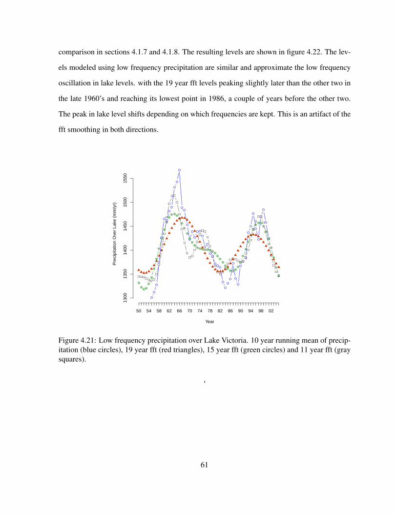
Examining the values for precipitation over the lake (Fig. 4.18 ), there is a decadal oscilla-
tion. We filtered the precipitation over Lake Victoria calculated from the interpolation of CRU
gridded precipitation, with no EOF filtering, to the six stations (section 3.5) using a 10 year
running mean and fft analysis, where we then reconstructed the precipitation using frequencies
below 11 years, 15 years and 19 years (Fig. 4.21). Since the 10 year running mean causes
data loss at both ends of the time series, only the reconstructed fft time series were used as
input to the water balance model in order to start the water balance model using 1949 levels for
60
comparison in sections 4.1.7 and 4.1.8. The resulting levels are shown in figure 4.22. The lev-
els modeled using low frequency precipitation are similar and approximate the low frequency
oscillation in lake levels. with the 19 year fft levels peaking slightly later than the other two in
the late 1960’s and reaching its lowest point in 1986, a couple of years before the other two.
The peak in lake level shifts depending on which frequencies are kept. This is an artifact of the
fft smoothing in both directions.
Year
Pre
cipi
tatio
n O
ver
Lake
(m
m/y
r)
1300
1350
1400
1450
1500
1550
50 54 58 62 66 70 74 78 82 86 90 94 98 02
Figure 4.21: Low frequency precipitation over Lake Victoria. 10 year running mean of precip-itation (blue circles), 19 year fft (red triangles), 15 year fft (green circles) and 11 year fft (graysquares).
,
61
Year
Lake
Lev
el (
m)
50 54 58 62 66 70 74 78 82 86 90 94 98 02
10.5
11.0
11.5
12.0
12.5
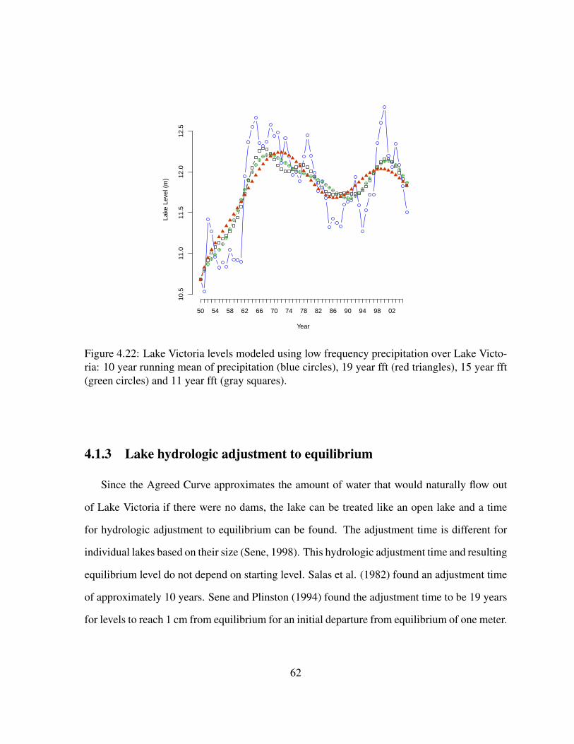
Figure 4.22: Lake Victoria levels modeled using low frequency precipitation over Lake Victo-ria: 10 year running mean of precipitation (blue circles), 19 year fft (red triangles), 15 year fft(green circles) and 11 year fft (gray squares).
4.1.3 Lake hydrologic adjustment to equilibrium
Since the Agreed Curve approximates the amount of water that would naturally flow out
of Lake Victoria if there were no dams, the lake can be treated like an open lake and a time
for hydrologic adjustment to equilibrium can be found. The adjustment time is different for
individual lakes based on their size (Sene, 1998). This hydrologic adjustment time and resulting
equilibrium level do not depend on starting level. Salas et al. (1982) found an adjustment time
of approximately 10 years. Sene and Plinston (1994) found the adjustment time to be 19 years
for levels to reach 1 cm from equilibrium for an initial departure from equilibrium of one meter.
62
While their calculations give different results, it is clear that the hydrologic adjustment time
is on a decadal time scale. The changes in equilibrium levels are considered in this study to
be a result of changes in the long term mean in precipitation over the lake basin and deviation
from the Agreed Curve. However, it should be taken into account when interpreting lake levels.
Comparing the water balance model run with the average precipitation over the lake before the
1961 jump, to the model run with average precipitation from 1965-2005, after the jump (Fig.
4.23) there is a new regime in precipitation with a higher average after 1965, even without
the four years of consistent, above average precipitation. Starting the water balance model in
1964 and using the mean 1964-1990 precipitation shows a decrease in levels about equal to the
average decrease in actual levels during this time as the lake levels reach a new equilibrium
consistent with the new mean precipitation after the peak in rainfall and level (Fig. 4.24).
Year
Lake
Lev
el (
m)
49 53 57 61 65 69 73 77 81 85 89 93 97 01 05
10.5
11.0
11.5
12.0
12.5
13.0
Figure 4.23: Lake Victoria levels modeled using pre-jump (1950-1960) (green) and post jump(1965-2005) (black) average precipitation over Lake Victoria compared to levels modeled usingCRU precipitation (blue).
63
Year
Lake
Lev
els
(m)
11.6
11.8
12.0
12.2
12.4
12.6
12.8
63 66 69 72 75 78 81 84 87 90
Figure 4.24: Lake Victoria levels modeled starting in 1963 using 1964-90 mean station gaugeprecipitation (black) and actual lake levels (blue).
4.1.4 Outflow from dams violating the Agreed Curve
While several studies have investigated the possibility of the violation of the agreed curve
by the outflow from Owen’s Falls Dam, as one of the explanations for the 1961-64 increase in
Lake Victoria Levels Kite (1981) showed using published excesses and shortages of released
water on an annual basis for 1957-1979, that dam usage has caused a cumulative rise in lake
level of just under 3 cm (Table 4.1). From 1961-1979, the table shows an excess release which
would decrease Lake Victoria levels during this time. Sene and Plinston (1994) examined
recorded releases from the Owen Falls dam site and compared those to expected releases from
the extended Agreed Curve (Fig. 4.25). They found that since operations started at the Owen
Falls dam, releases have followed the Agreed Curve for the most part and compensatory re-
leases have usually been made at a later date when departures have occurred. They found that
64
the effects of the departures from the Agreed Curve were small up to 1994. More recently, Kull
(2006(a) investigated the drop in Lake Victoria levels from 2002-2005, using a water balance
simulation for 2004 and 2005. He found that the severe drops in levels from 2004-2005 were
approximately 45% due to drought and 55% due to over-releases from Nalubaale and Kiira
dams. Kull (2006(a) extended these results by sampling technical reports and interviews from
2005 to compare reported dam releases to estimated lake levels from USDA (2005).
Table 4.1: Possible effect of Owen Falls Dam on Lake Victoria levels adapted from (Kite,1981), his Table 2.
Year Excess (+) or shortage (-) inRiver Nile flows (106m3)
Possible increase (+) ordecrease (-) in natural level of
Figure 4.25: Comparison of expected outflow based on the extended Agreed Curve (RecordA) and recorded releases from the Owen Falls dam (Record B) from Sene and Plinston (1994).
4.1.5 Modulation due to changes in land and water use
The water balance model estimates tributary inflow using a linear regression between the
runoff coefficient and subcatchment rainfall which are estimated from rainfall directly over the
lake. Changes in land and water use in the catchments could change these relationships in
the future. For example, more water could be used from the tributaries for irrigation before it
reaches the lake or deforestation could change the runoff coefficient and alter the climate of
the basin. In retrospect, based on our results, the contribution of this factor is relatively minor.
Moreover, further investigation of this factor is beyond the scope of this study.
4.1.6 Bottom sedimentation, thermal expansion, and changes in ground-
water
Several factors have not been studied fully in estimating Lake Victoria levels. Among these
are sedimentation accumulation at the bottom of the lake, changes in groundwater, and thermal
expansion from warming lake water.
66
Kayombo and Jorgensen (2007) found a rate of sediment accretion of 1 mm/yr. Swallow
et al. (2001) showed the sedimentation rate at the river inlets in the catchment area was 1 cm/yr,
suggesting that sediment accumulates at the lake shore. The effect of groundwater is assumed
to be negligible due to the absence of data (Krishnamurthy and Ibrahim; Piper et al., 1986).
In retrospect, based on our results, the contribution of these factors are relatively minor.
Moreover, further investigation of these factors is also beyond the scope of this study.
4.1.7 Relative contribution of different factors to Lake Victoria level jump
1960-64
The percentage of DL was calculated by dividing the change in level from 1960-64 using
the time series of the mode under investigation by the change in level for the same years in
the water balance model using CRU. All water balance model runs were started in 1949 and
run through 2005. Since the decadal harmonic was performed on the full precipitation data
set instead of individual EOF modes, the decadal harmonic is subtracted from the EOF mode
time series in order to separate the two factors before running the water balance model. The
change in levels for release, construction and sediment were estimated using the references in
table 1. We estimated the effect of over- and under-release by adding the possible increase or
decrease in the level of Lake Victoria from 1961 through 1964 found in table 2 of Kite (1981).
The possible changes in level found by Kite (1981) for each year equal are assumed to be small
enough that they do not affect Agreed Curve outflow.
Table 4.3 shows that the first mode of variability from the EOF analysis on CRU annual
precipitation accounts for between 28% and 43.7% of the jump from 1961-64 once the decadal
mode is removed, while the decadal mode accounts for between 18.4 and 34.2% of the jump.
These two modes account for 62% of the jump, no matter what wavelengths were kept in the
67
fft analysis. The remaining modes each account for less than 10% of the jump, with release
from the Nalubaale dam reducing the jump by half of a percent.
4.1.8 Relative contribution of factors to Lake Victoria level decline 1965-
2005
We focus on the drop in levels from 1965-2005 using the same technique described in
section 4.1.7. Using CRU in the water balance model, the level drops by 0.86 meters during
this time, while the satellite altimetry derived levels show a drop of 1.7 meters. There is a large
discrepancy between modeled levels and actual lake levels from 1997 to 2005, with the model
predicting higher than actual levels during these years. Without further information on releases
from Nalubaale and Kiira dams, we are unable to determine the cause of this discrepancy. The
main cause of the decrease in levels is the lake reaching a new equilibrium in response to mean
precipitation from 1965-2005 being lower than the four years of extreme precipitation which
caused the jump in levels investigated in section 4.1.7. This accounts for approximately 73% of
the decline in levels from 1965-2005 4.4. The remaining factors each account for less than 10%
of the decline. Even though ENSO/IOZM account for a majority of the interannual variability
in lake levels, the decadal oscillation accounts for more of the decline than ENSO/IOZM.
Table 4.2: Calculations to determine contribution of factors mentioned in section 4.1 to changesin Lake Victoria levels from 1949-64 and 1965-96.
Factor Data/Source Method output uncertainty
Decadal CRU (1950-2005) decadal filter (19 year fft filter) % of total ΔL changing window of filter (eg 10,15, 20 yr cycle)ENSO/IOZM CRU annual EOF 1 time series in WBM-decadal harmonic % of total ΔL subtraction of decadal modeAdjustment CRU result of previous lake level and precipitation over lake basin % of total ΔL
Trend CRU linear regression in R % of total ΔL (depends on time frame)Over/under release citation Kite (1981); Sene and Plinston (1994); Kull (2006(a,()
Construction citation Kite (1981); Sene and Plinston (1994)land/water cover area; deforestation believed to be smallΔL due to bottom sediment/soil erosion citation Kayombo and Jorgensen (2007) ~1 mm/yr
ΔV due to thermal expansion believed to be smallΔgroundwater citation Krishnamurthy and Ibrahim; Piper et al. (1986) believed to be small
68
Year
Leve
l (m
)
49 53 57 61 65 69 73 77 81 85 89 93 97 01 05
10.5
11.0
11.5
12.0
12.5
13.0
Figure 4.26: Effects of various modes of variability in Lake Victoria levels. Blue circles:CRU in the water balance model, Purple +’s: EOF first mode precipitation. minus decadalprecipitation. in water balance model, Red triangles: decadal, Black asterisks: trend from1950-2005 CRU in water balance model (similar to average over same time period), Greentriangles: 1950-1960 average precipitation. in water balance model.
Table 4.3: Estimation of amount of change in level, 1949-1964, covered by each factor men-tioned in section 4.1 and confidence.
mode % of total ΔL confidence
Decadal 18.4 between 18.4% and 34.2%ENSO/IOZM (EOF1) 43.5 (When 19 year fft is subtracted out) 58.1% w/ decadal included, between 28% and 43.7% w/ fft removed
Decadal + (EOF1 - Decadal) 62 +/- 0.3%Adjustment 7.8 (WBM reaching equilibrium using 1950-60 pre-jump mean) high
Trend 4.1 (1950-2005 trend) depends on when trend was takenOver/under release -0.5 very high
Construction included with Over/under release N/Aland/water cover area; deforestation considered small low, needs more studyΔL due to bottom sediment/soil erosion 0.2 high
ΔV due to thermal expansion 0 (very small) low, beyond scope of studyΔgroundwater 0 (very small) low, beyond scope of study
69
Table 4.4: Estimation of amount of change in level, 1965-2005, covered by each factor men-tioned in section 4.1 and confidence.
mode % of total ΔL confidence
Decadal 3.3% between -4 and 6.8%ENSO/IOZM (EOF1) 0 (When 19 year fft is subtracted out) 13.4 w/ decadal included, between -2% and 0% w/ fft removed
Decadal + (EOF1 - Decadal) 4 +/- 2.8%Adjustment 73.1 (WBM reaching equilibrium using 1965-2005 post-jump mean) high
Trend -3.6 (1950-2005 trend) depends on when trend was takenOver/under release unable to determine low
Construction included with Over/Under release N/Aland/water cover area; deforestation considered small low, needs more studyΔL due to bottom sediment/soil erosion 0.2 high
ΔV due to thermal expansion 0 (very small) low, beyond scope of studyΔgroundwater 0 (very small) low, beyond scope of study
4.2 21st Century projection of Lake Victoria Levels
To estimate the projected changes in the levels of Lake Victoria in response to climate
change, we used the projected rainfall from two primary sources. One source is the downscaled
FvGCM rainfall using the RegCM3 model (Bowden, 2008). As explained in section 3.5 for
CRU data, the gridded rainfall is interpolated to six stations to provide input to the Water
Balance Model. The second source are the IPCC ensemble projections described in section
2.6.
Figure 4.27 shows the preliminary results based on downscaling of the FvGCM global
model projection simulations using RegCM3. The regional model projections reveal details
which are not in the FvGCM and the average of 9 AR4 global model projections where all
the IPCC models exhibit wetter conditions throughout the region. Based on these preliminary
results, it is clear that the largest projected climate change signal in the interior of East Africa is
located over the Lake Victoria basin for all the three types of climate change projections. The
regional climate model (RegCM3), the FvGCM (1 degree resolution) and the coarser resolution
9 member IPCC GCM ensemble average agree on this outcome. However, the intensity of the
signal gets larger with increasing resolution and it is weakest with the IPCC AR4 ensemble
70
average. Since all three models show similar features, specifically around the lake basin, we
feel confident using their output in the water balance model.
Since the lake level in 2070 is unknown, several initial conditions are used in modeling
Lake Victoria levels from 2071-2100. Figure 4.27 shows the resulting lake levels for RegCM3
and the IPCC ensemble projections. FvGCM is not shown due to similarity to RegCM3 results.
The future levels from all three models give projected lake levels of 14 to 16 meters. The higher
resolution RegCM3 gives higher lake levels due to the larger amount of intensity in the signal
over the lake. There is also more variability in the regional climate model (RegCM3) due to
the fact that it is one model run, while the IPCC AR4 ensemble is an ensemble of 9 model
ensembles which filters out any variability in the time series of precipitation over the lake.
While these levels are almost 2 meters higher than the current lake levels and over a meter
higher than the 12.91 maximum lake level in December 1963, the lake level has reached an
average level of approximately 14 meters during 1876 to 1880, as reported by missionaries at
Buganda and shown in figure 4.2 (Nicholson, 1998).
We take the more conservative 14 meter increase from the IPCC AR4 ensemble and map
the flooding that increase would cause in ESRI ArcMap. This is done by first mapping a
SRTM 90 m resolution digital elevation model of the area downloaded from http://edcsns17.
cr.usgs.gov/EarthExplorer/. The current levels are 11.9 m (1,134 meters above sea level) at
Jinja gauge, which is the level Riebeek (2006) states the lake stayed above this level until
December 2005 when the levels dropped rapidly. The current (11.9 m) and future (14 m) lake
levels are then converted from heights at Jinja gauge to heights above sea level, considering
the Jinja gauge to be 1122.1 m above sea level. The values from the DEM are then subtracted
from the current and future lake heights using the raster calculator tool in the Spatial Analyst
toolbox. Positive values are considered to be under water and negative values are not. Figure
4.30, shows the result of this analysis for the entire lake. There will be more flooding in NW
sector of lake, so we will focus on this region. Figure 4.31 shows projected flooding on the
northwest side of Lake Victoria if levels reach 14 meters. The flooding focuses on the area
around Masaka. Figure 4.32 shows flooding near Kampala in Nakivubo wetland. While these
areas are mostly swamp, there has been encroachment on this flood land by people who build
houses and businesses in these locations. Nakivubo wetland is also used for sewage control
(Kyambadde et al., 2004). A railroad track near Fort Bell, Uganda is among the areas that
would be flooded.
The modeled A2 scenario levels can be used when planning for future use of hydroelectric
dams. Power Planning Associates (2007) recommended a new “constant release” or “Agreed
Curve by steps” rule for releasing water from Kiira and Nalubaale dams while working on
Bujagali II dam proposals. This rule was suggested in order to follow the Agreed Curve but al-
lowing for a constant release to be applied when the lake fluctuates within a certain range. They
recommend a “low hydrology” scenario where the mean release from Lake Victoria should be
kept around a value of 687 m3/s when the lake level is between 1133.5 and 1135.0 meters
above sea level (between 10.64 and 12.14 m at Jinja gauge) and an “high hydrology” scenario
where the mean release is kept near 1247 m3/s when the lake level is sustained above 1135
meters above sea level (12.14 m at Jinja gauge). Power Planning Associates base the “high
hydrology” scenario on the 1961-64 levels, followed by approximately 35 years with an aver-
age net inflow of 1200 m3/s during the entire period. The current Agreed Curve rule release
is between 1300 m3/s and 1400 m3/s in the water balance model for the projected lake levels
of around 14 meters. A new higher release scenario should be created for this scenario as a
release of less than that amount would cause lake levels to increase even further. This scenario
should be taken into account while a new Nile Basin treaty is being formed to share Nile River
water between Egypt, Sudan, Ethiopia, the Democratic Republic of Congo, Uganda, Tanzania,
Kenya, Burundi and Rwanda.
72
This information is potentially highly valuable over the River Nile basin in predicting future
outflow from Lake Victoria which could be used to assess future use of hydroelectric dams and
other applications such as land use and infrastructure planning over Lake Victoria basin.
Figure 4.27: Rainfall projections (A2: 2071-2100 average) minus (RF: 1961-1990 average) forthe Oct-Dec short rains: (left) RegCM3 (40 km grid); (center) 2-member FvGCM ensembleaverage); (right) IPCC GCM super ensemble average. Units (mm).
Figure 4.28: From Nicholson (1998). Fluctuations of Lake Victoria from 1780. Years withlevels determined from specific references have dots above them. Levels since 1896 are basedon modern measurements.
73
Figure 4.29: 2070-2099 Lake Victoria levels modeled using A2 scenario IPCC ensemble pre-cipitation.
56,000 0 56,00028,000 Meters
Potential Flooding Around Lake Victoria
Legend
Land
Potential Flooding
Current Lake
Figure 4.30: Projected flooding of Lake Victoria shores if lake level rises to 14 meters.
74
9,750 0 9,7504,875 Meters
Flooding around northwest side of Lake Victoria
Legend
road
Lake
Increase
Current Lake
Figure 4.31: Projected flooding on Northwest side of Lake Victoria if lake level rises to 14meters.
75
Entebbe
5,600 0 5,6002,800 Meters
Flooding near Kampala, Uganda
Legend
railroad
road
Lake
Increase
Current Lake
Figure 4.32: Projected flooding near Kampala, Uganda if lake level rises to 14 meters.
76
4.3 Seasonal Variability of Station Precipitation
In this section we (i) reproduce the EOF modes of Schreck and Semazzi (2004) using
station precipitation over Eastern Africa and then (ii) investigate the significant modes of vari-
ability of precipitation from January-February, March-May, and June-September in terms of
the findings of Schreck and Semazzi (2004) and other studies. We relate these seasonal modes
to the annual modes used in section 4.1.1.
4.3.1 Confirmation of Schreck and Semazzi (2004)
The percentage of variability covered by each EOF mode of station precipitation for the
OND season is shown in figure 4.33. The first two modes are significant and account for just
under 58% of the variability. We will be examined these modes in detail.
The first mode of OND station precipitation variability has a loading which is mostly one
sign except for a couple of stations to the south of the lake (Fig. 4.34). The time series we
obtain for the first mode of variability of OND station precipitation reproduces the time series
found by Schreck and Semazzi (2004) (Fig. 4.38). Schreck and Semazzi (2004) mention
that for a larger region using CMAP gridded precipitation, the first mode explained 29% of
variability, while a study by Nyenzi (1992) based on a smaller region covering only Uganda,
Kenya and Tanzania had a corresponding mode which had a variance of 50%. They believed
the difference in variability could be attributed to the larger region they used for the analysis
of CMAP precipitation. Our first mode explains 51.7% of the variability, which supports this
finding. Schreck and Semazzi (2004) relate their EOF1 to ENSO by correlating their time
series with the first significant EOF mode from global CMAP precipitation. They find that the
first mode from the EOF analysis on regional precipitation corresponds to a combination of
the first global EOF mode representing ENSO and the second global mode (IOZM). The major
77
warm ENSO events for the period covered by the station data correspond to the low valleys of
the time series. In particular the ENSO of 1982 is distinctly conspicuous. When the first mode
from OND precipitation is correlated with SSTs for 1961-1990, an Indian Ocean Dipole mode
pattern emerges (Fig 4.35). However, when they are correlated without 1961, an ENSO pattern
emerges (Fig. 4.36). This implies that the strong IOZM event that happened in 1961 was so
anomalous that it influenced the EOF analysis. This mode has a high correlation (0.82) with
the first annual mode from station precipitation from section 4.1.1. The first annual mode is
ENSO with some influence from IOZM, particularly in 1961.
Similar to Schreck and Semazzi (2004), the second mode of variability for station precip-
itation is significant. The second mode is a dipole mode with negative loading to the north
and positive loading to the south, which split the stations used in the water balance model in
section 4.1.1 with the stations to the east of the lake having negative loadings and those on the
western coast of the lake having positive loadings. The corresponding time series exhibits both
strong interannual variability and low-frequency background variability (Fig. 4.39). Overall,
there is an increasing trend during the entire time period. To explore possible associations with
global warming, Schreck and Semazzi (2004) plotted their Gauge EOF2 time series with the
global warming index (GWI). A 5 year running mean was applied to each of the time series
to filter out high frequencies and focus on low frequency variability (Fig. 4.40). Applying a
5 year running mean to our second mode time series gives the same time series (Fig. 4.41).
Combined interpretation of the distribution of loadings and the corresponding time series sug-
gests that the southern sector of eastern Africa has been getting wetter for the period 1961 to
1990 while the northern section has been drying up. This is opposite to the dipole described by
Schreck and Semazzi (2004) who claim that the nothern sector has been getting wetter while
the southern sector has been drying up. While our time series is the same as the time series
in Schreck and Semazzi (2004), our loadings are the inverse of theirs. To determine if there
78
is a problem with our EOF analysis we procede to do an EOF analysis of CRU precipitation
over Eastern Africa for the OND season 1979-2001 similar to that done for the Regional-EOF
analysis using CMAP in Schreck and Semazzi (2004). Examining the second EOF mode of
this analysis and comparing it to Regional-EOF2 in their paper (not shown), we obtain simi-
lar results to the Regional-EOF2 dipole with moistening to the north and drying to the south
(Fig. 4.42). This proves that there are no errors in our EOF calculations, at least for gridded
CRU precipitation. Comparing the second EOF modes for CRU precipitation data for the OND
season from 1961-90 (Fig. 4.44), to those from station gauge precipitation (Fig. 4.39) the load-
ings are similar, with negative loadings to the north and positive loadings to the south There is
a 0.75 correlation between the time series from the EOF analysis of CRU and the EOF analysis
of station gauge precipitation for the OND season 1961-90. We find that Schreck and Semazzi
(2004) must have inverted their Gauge-EOF2 loading. In order to determine source of vari-
ability associated with the second mode, we correlated it with SST anomalies (Fig. 4.45). The
areas of significant correlation focus towards the Bering Strait. We do not see any connection
between the SSTs in this area and East African rainfall. It could be a spurious correlation, but
should be investigated in the future. This mode has a 0.53 correlation with the second annual
mode from section 4.1.1 which suggests that it might be related to the second annual mode, but
other seasons might have more influence on this mode.
79
0.0
0.1
0.2
0.3
0.4
0.5
Station OND
Figure 4.33: Scree Plot OND Station EOF
80
Year
−10
010
2030
61 64 67 70 73 76 79 82 85 88
Station OND EOF 1
42°0’0"E
42°0’0"E
40°0’0"E
40°0’0"E
38°0’0"E
38°0’0"E
36°0’0"E
36°0’0"E
34°0’0"E
34°0’0"E
32°0’0"E
32°0’0"E
30°0’0"E
30°0’0"E
4°0’0"N 4°0’0"N
2°0’0"N 2°0’0"N
0°0’0" 0°0’0"
2°0’0"S 2°0’0"S
4°0’0"S 4°0’0"S
6°0’0"S 6°0’0"S
8°0’0"S 8°0’0"S
10°0’0"S 10°0’0"S
12°0’0"S 12°0’0"S
14°0’0"S 14°0’0"S
16°0’0"S 16°0’0"S
Legend
PrecipStations
-0.020332-0.01999
0.02-0.110032
Figure 4.34: Station OND EOF1 time series (top) and loading (bottom). Blue circles arepositive, yellow circles are neutral. Stations used in the WBM are marked with a star.
Figure 4.36: First mode from OND EOF analysis on station precipitation correlated withERSST from 1962-90.
82
Figure 4.37: Stations used in Schreck and Semazzi (2004).
Year
−10
010
2030
61 64 67 70 73 76 79 82 85 88
OND EOF 1
Figure 4.38: Station OND EOF1 time series (left) and Gauge OND EOF1 time series fromSchreck and Semazzi (2004)their figure 8 (right)
83
Year
−4
02
46
8
61 64 67 70 73 76 79 82 85 88
Station OND EOF 2
42°0’0"E
42°0’0"E
40°0’0"E
40°0’0"E
38°0’0"E
38°0’0"E
36°0’0"E
36°0’0"E
34°0’0"E
34°0’0"E
32°0’0"E
32°0’0"E
30°0’0"E
30°0’0"E
4°0’0"N 4°0’0"N
2°0’0"N 2°0’0"N
0°0’0" 0°0’0"
2°0’0"S 2°0’0"S
4°0’0"S 4°0’0"S
6°0’0"S 6°0’0"S
8°0’0"S 8°0’0"S
10°0’0"S 10°0’0"S
12°0’0"S 12°0’0"S
14°0’0"S 14°0’0"S
16°0’0"S 16°0’0"S
Legend
PrecipStations
-0.163818 - -0.020000
-0.019999 - 0.020000
0.020001 - 0.202505
Figure 4.39: Station OND EOF2 time series (top) and loading (bottom). Blue circles arepositive, yellow circles are neutral, red circles are negative. Stations used in the WBM aremarked with a star.
84
Figure 4.40: From Schreck and Semazzi (2004), Gauge-EOF 2 time series and loading. Theirfigures 12(b) and 13.
Figure 4.41: 5 year running mean of time series from OND EOF2.
85
Year
−10
010
20
1979 1982 1985 1988 1991 1994 1997 2000
42°0’0"E
42°0’0"E
40°0’0"E
40°0’0"E
38°0’0"E
38°0’0"E
36°0’0"E
36°0’0"E
34°0’0"E
34°0’0"E
32°0’0"E
32°0’0"E
30°0’0"E
30°0’0"E
4°0’0"N 4°0’0"N
2°0’0"N 2°0’0"N
0°0’0" 0°0’0"
2°0’0"S 2°0’0"S
4°0’0"S 4°0’0"S
6°0’0"S 6°0’0"S
8°0’0"S 8°0’0"S
10°0’0"S 10°0’0"S
12°0’0"S 12°0’0"S
14°0’0"S 14°0’0"S
16°0’0"S 16°0’0"S
Legend
PrecipStations
CRU 1979-2001 EOF 2
-0.063538 - -0.015000
-0.014999 - 0.015000
0.015001 - 0.072153
Figure 4.42: Second EOF mode from CRU OND 1979-2001 time series (top) and loading(bottom) .
86
Figure 4.43: Second EOF mode from CMAP OND 1979-2001 time series (top) and load-ing (bottom) from Schreck and Semazzi (2004). Their figure 5(b) and 6(b). For the loadingdark/light gray represents positive/negative values.
87
Year
−15
−5
05
1015
61 64 67 70 73 76 79 82 85 88
CRU 3.0 OND EOF 2
42°0’0"E
42°0’0"E
40°0’0"E
40°0’0"E
38°0’0"E
38°0’0"E
36°0’0"E
36°0’0"E
34°0’0"E
34°0’0"E
32°0’0"E
32°0’0"E
30°0’0"E
30°0’0"E
4°0’0"N 4°0’0"N
2°0’0"N 2°0’0"N
0°0’0" 0°0’0"
2°0’0"S 2°0’0"S
4°0’0"S 4°0’0"S
6°0’0"S 6°0’0"S
8°0’0"S 8°0’0"S
10°0’0"S 10°0’0"S
12°0’0"S 12°0’0"S
14°0’0"S 14°0’0"S
16°0’0"S 16°0’0"S
Legend
PrecipStations
loadings
-0.065254 - -0.021110
-0.021109 - 0.021943
0.021944 - 0.086587
Figure 4.44: CRU 3.0 OND EOF2 time series (top) and loading (bottom)
Figure 4.45: Second mode from OND EOF analysis on station precipitation correlated withERSST from 1961-90.
4.3.2 Extension of Schreck and Semazzi (2004) to other seasons
In order to examine the effects of each season on the annual EOF analysis performed in
section 4.1.1 and to Lake Victoria levels, we extend the analysis of Schreck and Semazzi (2004)
to the long rains of March through May and the dry seasons of January through February and
June through September.
4.3.2.1 March-May (MAM)
According to Indeje et al. (2000), about 42 percent of the total east African rainfall is
observed during the MAM season. The highest intensity is observed near the Indian Ocean,
Lake Victoria, and the East African Highlands. In MAM season, there are two significant
modes of variability for station precipitation (Fig. 4.46) the first mode accounts for 23.6% of
89
variability for station precipitation. The loading is negative in southern Tanzania and is split
across the lake with negative loadings on the western coast of Lake Victoria and positive on the
eastern coast of the lake and into the Kenya highlands (Fig. 4.47). The stations used in the water
balance model have mostly small near-zero to larger positive loadings. Combined analysis of
the time series and corresponding loadings for the stations used in the water balance model
indicate that this mode would contribute to the interannual variability of the lake, but there
is no definite trend. The time series has no correlation with the OND first mode time series
(0.056 correlation) or the second mode (0.205). However it does have a 0.526 correlation with
the first mode of annual station precipitation from section 4.1.1. We investigate the source of
variability for the mode by correlating it with SST over the globe and find that there are high
correlations in the area off the pacific coast of Central America and northern South America
(Columbia, Ecuador, Peru). There is a small horseshoe pattern in the Pacific Ocean similar to
an ENSO pattern (Fig. 4.48). The second mode for this season accounts for 10.9% variability.
It is positive to the north and east coasts of the lake, and in northern Uganda and western Kenya
with a negative loading in southern Kenya and eastern Tanzania (Fig. 4.49). The loading is
similar to the loading for the first mode, but with a shift in negative loadings northward. This
mode is not well correlated with either the first or second modes from OND precipitation (-0.10
and -0.37 correlations respectively). However it is highly correlated (-0.74) with the second
mode of variability of annual precipitation from section 4.1.1. Correlating the time series with
SST anomalies shows a negative correlation with temperatures in the Arabian Sea and off the
coast of Taiwan and the Philippines in the Pacific Ocean.
90
0.00
0.10
0.20
Station MAM
Figure 4.46: Scree Plot MAM Station EOF
91
Year
−10
−5
05
10
61 64 67 70 73 76 79 82 85 88
Station MAM EOF 1
42°0’0"E
42°0’0"E
40°0’0"E
40°0’0"E
38°0’0"E
38°0’0"E
36°0’0"E
36°0’0"E
34°0’0"E
34°0’0"E
32°0’0"E
32°0’0"E
30°0’0"E
30°0’0"E
4°0’0"N 4°0’0"N
2°0’0"N 2°0’0"N
0°0’0" 0°0’0"
2°0’0"S 2°0’0"S
4°0’0"S 4°0’0"S
6°0’0"S 6°0’0"S
8°0’0"S 8°0’0"S
10°0’0"S 10°0’0"S
12°0’0"S 12°0’0"S
14°0’0"S 14°0’0"S
16°0’0"S 16°0’0"S
Legend
PrecipStations
-0.051583 - 0.027675
0.027676 - 0.092422
0.092423 - 0.149697
Figure 4.47: Station MAM EOF1 time series (top) and loading (bottom). Blue circles arepositive, yellow circles are neutral, red circles are negative. Stations used in the WBM aremarked with a star.
Figure 4.48: First mode from MAM EOF analysis on station precipitation correlated withERSST from 1961-90.
93
Year
−5
05
61 64 67 70 73 76 79 82 85 88
Station MAM EOF 2
42°0’0"E
42°0’0"E
40°0’0"E
40°0’0"E
38°0’0"E
38°0’0"E
36°0’0"E
36°0’0"E
34°0’0"E
34°0’0"E
32°0’0"E
32°0’0"E
30°0’0"E
30°0’0"E
4°0’0"N 4°0’0"N
2°0’0"N 2°0’0"N
0°0’0" 0°0’0"
2°0’0"S 2°0’0"S
4°0’0"S 4°0’0"S
6°0’0"S 6°0’0"S
8°0’0"S 8°0’0"S
10°0’0"S 10°0’0"S
12°0’0"S 12°0’0"S
14°0’0"S 14°0’0"S
16°0’0"S 16°0’0"S
Legend
PrecipStations
-0.188331 - -0.030000
-0.029999 - 0.030000
0.030001 - 0.117095
Figure 4.49: Station MAM EOF2 time series (top) and loading (bottom). Blue circles arepositive, yellow circles are neutral, red circles are negative. Stations used in the WBM aremarked with a star.
Figure 4.50: Second mode from MAM EOF analysis on station precipitation correlated withERSST from 1961-90.
4.3.2.2 January-February (JF)
There is only one significant mode of variability during the January-February season which
accounts for 27% variability. The loading is positive over the entire East African region as seen
in figure 4.52. The time series has low frequency variability with a high amount of interannual
variability for the first half of the period, but less variability after 1980. Combined interpreta-
tion of the distribution of loadings and the corresponding time series suggests that during the
JF season, the entire area was wetter in the 1960’s and early 1970’s, with a dry period from
1973-76, a very wet period from 1977-79, and from 1980 has been recovering from a dry pe-
riod. Correlation with SST anomalies shows that this mode is related to SST anomalies in the
Indian Ocean, where warmer temperatures in the western Indian Ocean cause this season to
become wetter. This mode is not correlated with either of the OND modes of variability, and
only has a 0.30 correlation with the first mode of variability for annual precipitation discussed
95
in section 4.1.1.
0.00
0.10
0.20
0.30
Station JF
Figure 4.51: Scree Plot JF Station EOF
96
Year
−10
05
1015
61 64 67 70 73 76 79 82 85 88
Stations JF EOF 1
42°0’0"E
42°0’0"E
40°0’0"E
40°0’0"E
38°0’0"E
38°0’0"E
36°0’0"E
36°0’0"E
34°0’0"E
34°0’0"E
32°0’0"E
32°0’0"E
30°0’0"E
30°0’0"E
4°0’0"N 4°0’0"N
2°0’0"N 2°0’0"N
0°0’0" 0°0’0"
2°0’0"S 2°0’0"S
4°0’0"S 4°0’0"S
6°0’0"S 6°0’0"S
8°0’0"S 8°0’0"S
10°0’0"S 10°0’0"S
12°0’0"S 12°0’0"S
14°0’0"S 14°0’0"S
16°0’0"S 16°0’0"S
Legend
PrecipStations
0.009120 - 0.020000
0.020001 - 0.129911
Figure 4.52: Station JF EOF1 time series (top) and loading (bottom). Yellow circles are neutral,blue circles are positive. Stations used in the WBM are marked with a star.
Figure 4.53: First mode from JF EOF analysis on station precipitation correlated with ERSSTfrom 1961-90.
4.3.2.3 June-September (JJAS)
The JJAS rainfall season accounts for about 15% of the total regional annual rainfall (Indeje
et al., 2000). There are two significant modes of variability during this season. The first mode
accounts for 20 percent of the variability during this season (Fig. 4.54). The loading for
this mode is mostly negative, except for a few positive stations to the south of the lake (Fig.
4.55). The time series has very large negative peaks in 1961 and 1967, with otherwise smaller
interannual variability until the 1980’s. Correlation with SST anomalies does not give much
insight into the source of variability of this mode as shown in figure 4.56. The source of
variability of this mode is not related to SST. However, the correlation between the time series
of this mode and that of the first mode of the OND season is -0.433. This mode has a -0.40
correlation with the first mode of variability for annual precipitation mentioned in section 4.1.1.
The second mode accounts for 15.8 percent of the variability of precipitation during this
98
season. The loading for this mode is negative surrounding the lake and to the north into Uganda
and east halfway into Kenya while most of Tanzania and the southeastern portion of Kenya has
positive loadings (Fig. 4.57). The corresponding time series has large interannual variability
and a low frequency variability with a dip throughout the 1970’s reaching a minimum in 1975.
Combined analysis of the time series and corresponding loadings from the stations used in the
water balance model in section 4.1.1, show dry conditions over the lake in the 1960’s, followed
by moist conditions in the 1970’s and a return to drier conditions in the 1980’s. Correlation
with SST anomalies shows high correlation with a warm tongue in the pacific ocean and cooler
SSTs off the coast of Australia. This mode has a negative correlation with the first mode from
the OND season (0.407). While the time series of this mode has a negative correlation with
the time series from the first mode of annual precipitation from section 4.1.1 (0.30). It has a
higher, 0.64 correlation with the second mode of annual precipitation.
0.00
0.05
0.10
0.15
Station JJAS
Figure 4.54: Scree Plot JJAS Station EOF
99
Year
−15
−5
05
61 64 67 70 73 76 79 82 85 88
Stations JJAS EOF 1
42°0’0"E
42°0’0"E
40°0’0"E
40°0’0"E
38°0’0"E
38°0’0"E
36°0’0"E
36°0’0"E
34°0’0"E
34°0’0"E
32°0’0"E
32°0’0"E
30°0’0"E
30°0’0"E
4°0’0"N 4°0’0"N
2°0’0"N 2°0’0"N
0°0’0" 0°0’0"
2°0’0"S 2°0’0"S
4°0’0"S 4°0’0"S
6°0’0"S 6°0’0"S
8°0’0"S 8°0’0"S
10°0’0"S 10°0’0"S
12°0’0"S 12°0’0"S
14°0’0"S 14°0’0"S
16°0’0"S 16°0’0"S
Legend
PrecipStations
-0.162324 - -0.020000
-0.019999 - 0.020000
0.020001 - 0.063190
Figure 4.55: Station JJAS EOF1 time series (top) and loading (bottom). Blue circles are nega-tive, yellow circles are neutral, red circles are positive. Stations used in the WBM are markedwith a star.
Figure 4.56: First mode from JJAS EOF analysis on station precipitation correlated withERSST from 1961-90.
101
Year
−10
−5
05
61 64 67 70 73 76 79 82 85 88
Stations JJAS EOF 2
42°0’0"E
42°0’0"E
40°0’0"E
40°0’0"E
38°0’0"E
38°0’0"E
36°0’0"E
36°0’0"E
34°0’0"E
34°0’0"E
32°0’0"E
32°0’0"E
30°0’0"E
30°0’0"E
4°0’0"N 4°0’0"N
2°0’0"N 2°0’0"N
0°0’0" 0°0’0"
2°0’0"S 2°0’0"S
4°0’0"S 4°0’0"S
6°0’0"S 6°0’0"S
8°0’0"S 8°0’0"S
10°0’0"S 10°0’0"S
12°0’0"S 12°0’0"S
14°0’0"S 14°0’0"S
16°0’0"S 16°0’0"S
Legend
PrecipStations
-0.176186 - -0.020000
-0.019999 - 0.020000
0.020001 - 0.105264
Figure 4.57: Station JJAS EOF2 time series (top) and loading (bottom). Blue circles are nega-tive, yellow circles are neutral, red circles are positive. Stations used in the WBM are markedwith a star.
Figure 4.58: Second mode from JJAS EOF analysis on station precipitation correlated withERSST from 1961-90.
4.4 Decadal variability
In a new study by Clement et al. (Submitted), atmospheric models coupled to a mixed
layer ocean (with no coupled ocean dynamics) simulate what they refer to as an “Atmospheric
Walker Mode” which strongly resembles observed patterns associated with the SO. Their re-
sults suggest that there is power in the SO at decadal timescale, which can be thought of as the
combination of multiple processes: mixed-layer integration of trade wind variability, damping
by ocean dynamics, and a possible rectification of strong, non-linear interannual variability.
Clement et al. (Submitted) claim that Pacific climate anomalies that have an ’ENSO-like’ spa-
tial structure with warming in the eastern Pacific, eastward shift in convection, and a weaker
Walker circulation can develop on decadal timescales without dynamical coupling to the ocean.
In order to confirm the decadal Southern Oscillation recently found by Clement et al. (Submit-
103
ted) and investigate its impact on Eastern Africa, we perform an EOF analysis on OND season
1961-90 station gauge precipitation data filtered using a 10 year running mean analysis and
compared the results. We then examine the significant modes of variability for the filtered
precipitation as we did for the non-filtered precipitation.
There are three significant modes of variability for the low frequency OND season (Fig.
4.59) accounting for a total of 83.9 percent of the variability. The first mode of low frequency
OND precipitation accounts for 45.7 percent of the variability. The loading is mostly negative
except for two stations towards the northeast corner of the lake, one station near the border
of Uganda and Rwanda and two stations to the south of the lake with positive loadings (Fig.
4.60). The time series shows a very long term trend which increases from 1965-1972 and
then decreases until 1981. Combined interpretation of the distribution of the loadings and the
corresponding time series for this mode indicates that most of eastern Africa has gone from
being wet in the 10 years centered on 1965 followed by a drying trend which peaked in the
10 years centered on 1972, followed by increased wetness. Correlating the time series from
this mode with SST anomalies (Fig. 4.61) shows the ’ENSO-like’ signal described by Clement
et al. (Submitted) as seen in figure 4.62. In their analysis figure, three datasets are used here:
HadISST (Rayner et al. 2003), ERSSTv2, and ERSSTv3(Smith et al. 2008). They averaged
the three datasets in order to emphasize the patterns that are present in all datasets, but overall
the patterns do not change significantly from dataset to dataset. In parts c and d of the figure,
the stippling indicates areas that are not robust defined as where (1) the datasets do not agree in
sign and (2) where the regression values are not significant at the 1-sigma level (67%) based on
a t-test with reduced degrees of freedom to account for the auto-correlation in the filtered SO
index. All data are detrended and regressions computed for the 1880- 2004 period. This mode
shows a 0.79 correlation with a 10 year running mean taken of the Southern Oscillation Index
(SOI). This mode is the decadal Southern Oscillation found by Clement et al. (Submitted).
104
The second mode accounts for approximately 30 percent of the variability. The time series
for this loading is very linear, going from a low in 1965 to a peak in 1983 before decreasing
slightly (Fig. 4.63). While the stations used in the water balance model in section 4.1.1 all
have very small neutral to larger negative loadings, the pattern of the loadings splits the lake
with positive loadings on the western coast and negative loadings on the northern and eastern
coasts. Outside of the coast, there is a general pattern of negative loadings to the north and
more positive loadings to the south, similar to the loading for the second mode of annual
OND precipitation (Fig. 4.39). Combined interpretation of the distribution of the loadings
and the corresponding time series of this mode indicates that the areas on the north and east
sides of the lake are getting dryer while areas to the south of the lake are becoming moister.
Correlating the corresponding time series with SST anomalies in figure 4.64 shows very high
correlations with warm temperatures in the Indian Ocean and towards Antarctica and negative
correlations in the Pacific Ocean. There is an area of negative correlations between North
America and Europe which look like the gulf stream. The time series and correlation with SST
anomalies might be due to climate change, more research is needed to determine this. The
strong correlations are due to the EOF time series trend correlating highly with trends in SST
anomalies. Correlating two trends is risky and one has to be cautious that these two trends
could be physically unrelated.
The third mode, accounting for 8.3 percent of the variability, has low frequency variability
with a dip from 1965-1970, followed by a peak in the mid to late 1970’s and a decrease to 1983
(Fig. 4.66). The distribution of the loadings is noisier than the previous modes. There are both
positive and negative loadings around the coast of Lake Victoria. Overall the loading is very
noisy with positive and negative loadings scattered throughout the domain. The correlation of
the time series with SST anomalies does not give a distinctive pattern. Combined analysis of
the EOF loadings and the correlation of the time series with SST anomalies suggests that this
105
mode is not affected by SSTs and could be related to land use near the different stations in the
domain.
Bowden (2008) did a similar EOF analysis on a 10-year running mean of CRU for a larger
domain focusing on the Greater Horn of Africa (Fig. 4.65). He found that for the majority
of the Greater Horn of Africa, excluding portions of Tanzania and northern Sudan, the most
significant mode was a drying trend from the wetter 1960’s to near normal conditions during
the 1970’s, followed by a trend towards drier conditions in the early 1980’s. Since his domain
is much larger, it is hard to compare his mode to ours. However, his mode is similar to our
second mode which shows areas to the north of the lake becoming drier from 1960’s through
1980’s. It is possible that there was a different variability over the Greater Horn of Africa
than there was in the smaller Eastern Africa domain and the modes were ordered differently
between the two domains.
0.0
0.1
0.2
0.3
0.4
OND Running Mean
Figure 4.59: Scree Plot decadal OND Station EOF
106
Year
−15
−5
05
10
65 67 69 71 73 75 77 79 81 83 85
OND Running Mean EOF TS1
42°0’0"E
42°0’0"E
40°0’0"E
40°0’0"E
38°0’0"E
38°0’0"E
36°0’0"E
36°0’0"E
34°0’0"E
34°0’0"E
32°0’0"E
32°0’0"E
30°0’0"E
30°0’0"E
4°0’0"N 4°0’0"N
2°0’0"N 2°0’0"N
0°0’0" 0°0’0"
2°0’0"S 2°0’0"S
4°0’0"S 4°0’0"S
6°0’0"S 6°0’0"S
8°0’0"S 8°0’0"S
10°0’0"S 10°0’0"S
12°0’0"S 12°0’0"S
14°0’0"S 14°0’0"S
16°0’0"S 16°0’0"S
Legend
PrecipStations
-0.123359 - -0.010000
-0.009999 - 0.010000
0.010001 - 0.076508
Figure 4.60: Station OND 10 year running mean EOF1 time series (top) and loading (bottom).Blue circles are positive, yellow circles are neutral, red circles are negative. Stations used inthe WBM are marked with a star.
OND Running Mean TS1 Correlated with Running Mean of ERSST
Figure 4.61: First mode from OND 10 year running mean EOF analysis on station precipitationcorrelated with 10 year running mean of OND ERSST from 1961-90.
Figure 4.62: Regression of observed SLP on monthly observed (a) high and (b) low pass filtered(Butterworth filter, 10-yr cutoff) SO index using the HadSLP reconstruction version 2 (Allenand Ansell, 2006). Multidataset ensemble-mean regression on monthly observed (c) high and(d) low pass filtered SO index (Butterworth filter, 10-yr cutoff) index. All regressions wereperformed on the normalized SO, so units are hPa (for SLP) and K (for SST). From Clementet al. (Submitted) (their Figure 2)
108
Year
−10
−5
05
65 67 69 71 73 75 77 79 81 83 85
OND Running Mean EOF TS2
42°0’0"E
42°0’0"E
40°0’0"E
40°0’0"E
38°0’0"E
38°0’0"E
36°0’0"E
36°0’0"E
34°0’0"E
34°0’0"E
32°0’0"E
32°0’0"E
30°0’0"E
30°0’0"E
4°0’0"N 4°0’0"N
2°0’0"N 2°0’0"N
0°0’0" 0°0’0"
2°0’0"S 2°0’0"S
4°0’0"S 4°0’0"S
6°0’0"S 6°0’0"S
8°0’0"S 8°0’0"S
10°0’0"S 10°0’0"S
12°0’0"S 12°0’0"S
14°0’0"S 14°0’0"S
16°0’0"S 16°0’0"S
Legend
PrecipStations
-0.153125 - -0.030000
-0.029999 - 0.030000
0.030001 - 0.121764
Figure 4.63: Station OND 10 year running mean EOF2 time series (top) and loading (bottom).Blue circles are positive, yellow circles are neutral, red circles are negative. Stations used inthe WBM are marked with a star.
OND Running Mean TS2 Correlated with Running Mean of ERSST
Figure 4.64: Second mode from OND 10 year running mean EOF analysis on station precipi-tation correlated with 10 year running mean of ERSST from 1961-90.
110
Figure 4.65: Time series for the dominant EOF mode of variability for the 10-year runningmean analysis for 1961-90 time series (top) and loading (bottom) from Bowden (2008) .
111
Year
−4
−2
02
4
65 67 69 71 73 75 77 79 81 83 85
OND Running Mean EOF TS3
42°0’0"E
42°0’0"E
40°0’0"E
40°0’0"E
38°0’0"E
38°0’0"E
36°0’0"E
36°0’0"E
34°0’0"E
34°0’0"E
32°0’0"E
32°0’0"E
30°0’0"E
30°0’0"E
4°0’0"N 4°0’0"N
2°0’0"N 2°0’0"N
0°0’0" 0°0’0"
2°0’0"S 2°0’0"S
4°0’0"S 4°0’0"S
6°0’0"S 6°0’0"S
8°0’0"S 8°0’0"S
10°0’0"S 10°0’0"S
12°0’0"S 12°0’0"S
14°0’0"S 14°0’0"S
16°0’0"S 16°0’0"S
Legend
PrecipStations
-0.234218 - -0.030000
-0.029999 - 0.030000
0.030001 - 0.246326
Figure 4.66: Station OND 10 year running mean EOF3 time series (top) and loading (bottom).Blue circles are positive, yellow circles are neutral, red circles are negative. Stations used inthe WBM are marked with a star.
OND Running Mean TS3 Correlated with Running Mean of ERSST
Figure 4.67: Third mode from OND 10 year running mean EOF analysis on station precipita-tion correlated with 10 year running mean of ERSST from 1961-90.
113
Chapter 5
Conclusions and recommendations
5.1 Conclusions
We show that the jump in level from 1961-64 is due to 4 years of consistently above normal
precipitation associtated with the first mode of annual EOF variability, while the slow decline
from 1964-90 is primarily due to the adjustment of the lake levels to ’drier’ climatological
conditions contrary to conventional wisdom that climate change may have had a primary role
in determining this trend.
We find that the first EOF mode of annual precipitation variability (ENSO) has the highest
impact on the annual variability of Lake Victoria level. It has high correlation with the first
modes of variability during the OND and MAM seasons. While the second EOF mode of
annual variability accounts for approximately 10 percent of the variability, its effect on the
variability in lake levels is negligible. We further show that there was an error in the gauge-
2 EOF from Schreck and Semazzi (2004) and that contrary to their results for 1961-90, the
southern sector of eastern Africa was getting wetter for the period 1961 to 1990 while the
northern section was drying up. The corresponding time series for the dipole mode has a
114
0.532 correlation with the time series for the second EOF mode of annual precipitation for the
region. The annual dipole mode from CRU precipitation was contributing to a small overall
increase in Lake Victoria levels from 1961-90. This does not affect lake levels considerably
during that time period, as the lake is adjusting downwards toward a new equilibrium level
from the levels associated with the four years of consistantly high precipitation from 1961-
64 and the slight drying trend in the first mode of annual precipitation. The EOF analysis of
annual precipitation for 1961-90 has one sign of loading covering the lake for both CRU and
station gauge precipitation. The second EOF mode of annual precipitation variability has is
significantly correlated with the second EOF modes of variability from the OND, MAM, and
JJAS seasons. Based on the EOF analysis of OND season rainfall for the years 1961-1990 and
1979-2001 performed in section 4.3.1, the dipole is split with very small values over the lake
from 1961-1990 and 1979-2001. The dipole also splits with small values over the lake in the
MAM season, while in JJAS there are negative loadings surrounding the lake but the lake is
close to where the loadings switch to being positive, suggesting that they are smaller negative
loadings surrounding the lake. This suggests that another reason the dipole may have negligible
effect on Lake Victoria levels is that the loadings for the annual dipole are overall small since
in the OND and MAM seasons there are a combination of positive and negative loadings over
the lake that come close to cancelling out.
We reproduce the decadal SO studied by Clement et al. (Submitted) by correlating the first
mode of variance of the running mean of station gauge OND precipitation over Eastern Africa
to SST anomalies. The second mode has an increasing trend-like time series and negative
loadings around the lake. Combined analysis of the time series and loadings indicate a drying
trend around Lake Victoria.
115
5.2 Framework for use of climate change projections in ap-
plications
In section 4.2, we implement a framework for the use of climate change projections in the
application of hydrology. The framework is to first show that the water balance model gives
acceptable lake levels using observations. Next, climate model output is validated and then
used in the water balance model. Following this, the A2 scenario levels are converted to height
above sea level and ArcGIS software is used to map potential impacts of those levels. Our GIS-
based visualizations highlight the high threat of flooding of the wetlands in the coastal regions
of the lake which we believe would be a valuable tool for planners for climate adaptation and
mitigation.
5.3 Recommendations:
While the water balance model used in this study was designed to predict annual lake levels,
it would be useful for water resources and hydroelectric planning to have a corresponding
monthly analysis. This would require high quality monthly observations for all factors in
the water balance model including precipitation over the lake and in the lake basins, rates
of flow for all the tributaries into the lake, evaporation from the lake and the tributaries, and
groundwater flow. There is a definite need for sustained and improved monitoring of Lake
Victoria and its basin. While current lake levels can be estimated using satellite altimetry,
quality high resolution data for factors such as tributary inflow and groundwater is not available
for the Lake Victoria basin. There also needs to be an accounting of water taken from the lake
and it’s tributaries for human use in order to get a more accurate water balance.
It would be better to use dynamical water balance model which is could be run off of climate
116
model output for predicting lake levels under future climate change scenarios. The model used
by Tate et al. (2004) would be less reliable outside the regimes under which it was calibrated.
The regressions for runoff and tributary inflow into Lake Victoria could change with different
land use scenarios and climate regimes. These changes could be incorporated into a dynamical
model after it is calibrated using current conditions.
It would also be informative to calculate uncertainty over the entire chain of steps involved
in this study from uncertainty in the data used to uncertainty in the water balance model and
how this estimation of uncertainty cascades from data to impact. There is uncertainty from
choice of data sets used, the statistical analysis through the choices of spatial and temporal
domain for the EOF analysis and choice of filtering for the decadal analysis and the water
balance model itself. These uncertainties are filtered through into the predicted lake levels and
related impacts. This uncertainty could then be taken into account when planning for mitigation
of the potential impacts.
117
Bibliography
Allen, R. J. and T. J. Ansell, 2006: A new globally complete monthly historical mean sea levelpressure data set (HadSLP2): 1850-2004. Journal of Climate, 20, 667–680.
Anyah, R. O., S. F. H. M., and L. Xie, 2009: Hydrodynamic characteristics of Lake Victoriabased on idealized 3D lake model simulations. International Journal of Climatology, 29,971–981.
Anyah, R. O. and F. H. M. Semazzi, 2004: Simulation of the sensitivity of Lake Victoriabasin climate to lake surface temperatures. Theoretical and Applied Climatology, 79, 55–69,doi:10.1007/s00704-004-0057-4.
Anyah, R. O. and F. H. M. Semazzi, 2006: NCAR-AGCM ensemble simulations of the vari-ability of the Greater Horn of Africa climate. Special issue of Theoretical and Applied Cli-matology, 86, 39–62.
Anyah, R. O. and F. H. M. Semazzi, 2007: Variability of East African rainfall based on multi-year RegCM3 simulations. International Journal of Climatology, 27, 357–371.
Anyah, R. O., F. H. M. Semazzi, and L. Xie, 2006: Simulated physical mechanisms associatedwith climate variability over Lake Victoria Basin in East Africa. Monthly Weather Review,132 (12), 3588–3609.
Asnani, G. C., 1993: Tropical Meteorology. Prof. G. C. Asnani.
Asnani, G. C., 2005: Tropical Meteorology, (Revised Edition). Prof. G. C. Asnani.
Ba, M. B. and S. E. Nicholson, 1998: Analysis of convective activity and its relationship to therainfall over the Rift Valley Lakes of East Africa during 1983-90 using the Meteosat infraredchannel. Journal of Applied Meteorology, 37, 1250–1264.
Bowden, J. H., 2008: Multi-scale climate change modeling study over the Greater Horn ofAfrica. Ph.D. thesis, North Carolina State University.
Bowden, J. H. and F. H. M. Semazzi, 2007: Empirical analysis of intraseasonal climatevariability over the Greater Horn of Africa. Journal of Climate, 20 (23), 5715–5731, doi:10.1175/2007JCLI1587.1.
118
Clark, C. O., P. J. Webster, and J. E. Cole, 2003: Interdecadal variability of the relationshipbetween the indian ocean zonal mode and east african coastal rainfall anomalies. Journal ofClimate, 16 (3), 548–554.
Clement, A., P. DiNezio, and C. Deser, Submitted: Rethinking the ocean’s role in the southernoscillation. Journal of Climate.
Coppola, E. and F. Giorgi, 2005: Climate change in tropical regions from high-resolution time-slice AGCM experiments. Quarterly Journal of the Royal Meteorological Society, 131 (612),3123–3145, doi:10.1256/qj.04.166.
Davis, N. N., 2007a: Dynamic and stochastic modeling of various components of the hydro-logical cycle for East Africa. M.S. thesis, North Carolina State University.
Davis, N. N., 2007b: Dynamic and stochastic modeling of various components of the hydro-logical cyle for East Africa. M.S. thesis, North Carolina State University.
de Baulny, H. L. and D. Baker, 1970: The water balance of Lake Victoria. Tech. rep., UgandaMinistry of Water Development.
Flohn, H. and K. Fraedrich, 1966: Tagesperiodische zirkulation und niederschlagsverteilungam Victoria-See (Ostafrika) (the daily periodic circulation and distribution of rainfall overLake Victoria, in German). Meteorologische Rundschau, 19, 157–165.
Garretson, A., 1967: The Nile Basin, 256–258. Oceana Publications, Dobbs Ferry, NY.
Howell, P. P. and J. A. Allan, (Eds.) , 1994: The Nile: Sharing a Scarce Resource: A His-torical and Technical Review of Water Management and of Economical and Legal Issues.Cambridge University Press.
Howell, P. P., M. Lock, and S. Cobb, 1988: The Jonglei Canal : impact and opportunity. Cam-bridge studies in applied ecology and resource management, Cambridge University Press,URL http://www.worldcat.org/isbn/0521302862.
Indeje, M., F. H. M. Semazzi, and L. J. Ogallo, 2000: ENSO signals in East African rainfallseasons. International Journal of Climatology, 20 (1), 19–46.
Institute of Hydrology, 1985: Further review of the hydrology of Lake Victoria. report to theOverseas Development Administration. Wallingford, UK.
Janowiak, J. E., 1988: An investigation of interannual rainfall variability in Africa. Journal ofClimate, 1 (3), 240–255.
Kayombo, S. and S. E. Jorgensen, 2007: Lake Victoria: Experience and lessons learnedbrief. International Lake Environment Committee, Lake Basin Management Initiative., URLhttp://www.iwlearn.net/publications/ll/lakevictoria_2005.pdf, URL http://www.iwlearn.net/publications/ll/lakevictoria_2005.pdf.
Kendall, M., 1980: Multivariate Analysis. 2d ed., Hodder Arnold.
Kiehl, J. T., J. J. Hack, G. B. Bonan, B. A. Boville, and B. P. Briegleb, 1996: Description ofthe NCAR Community Climate Model (CCM3). Tech. rep., NASA.
Kite, G. W., 1981: Recent changes in level of Lake Victoria. Hydrological Sciences Bulletin,26 (3), 233–243.
Koren, V., 1995: Lake model. Nile Technical Notes no. 0154. Tech. rep., Nile Forecast Center,Ministry of Water Resources and Irrigation, Cairo, Egypt.
Krishnamurthy, K. V. and A. M. Ibrahim, ????: Washington, DC.
Kull, D., 2006(a): Connections between recent water level drops in Lake Victoria, dam opera-tions and drought. published online at http://www.irn.org/programs/nile/.
Kull, D., 2006(b): Addendum to: Connections between recent water leveldrops in Lake Victoria dam operations and drought. Published online athttp://www.irn.org/programs/nile/index.php?id=060614kull.html.
Kyambadde, J., F. Kansiime, L. Gumaelius, and G. Dalhammar, 2004: Hydraulic loading, sta-bility and water quality of Nakivubu wetland, Uganda. African Journal of Aquatic Science,29, 213–220.
Latif, M., et al., 1998: A review of the predictability and prediction of ENSO. Journal ofGeophysical Research, 103 (C7), 375–393, doi:10.1029/97JC03413.
Lin, S. J., R. Atlas, and K.-S. Yeh, 2004: Global weather prediction and high-end computingat NASA. Computing in Science & Engineering, 6 (1), 29–35, doi:10.1109/MCISE.2004.1255818.
Mangeni, B. T., 2006: The dwindling Lake Victoria water level. IASTED International Confer-ence Environmentally Sound Technology in Water Resources Management, O. Totolo, Ed.,ACTA Press, International Association of Science and Technology for Development, Vol.515-803, 85–90.
Mitchell, T. D. and P. D. Jones, 2005: An improved method of constructing a database ofmonthly climate observations and associated high-resolution grids. International Journal ofClimatology, 25, 693–712.
New, M., M. Hulme, and P. Jones, 2000: Representing twentieth-century space-time climatevariability. part ii: Development of 1901-96 monthly grids of terrestrial surface climate.Journal of Climate, 13, 2217–2238.
Nicholson, S. E., 1996: A review of climate dynamics and climate variability in eastern Africa.,25–56. Gordon and Breach, Amsterdam, The Netherlands.
Nicholson, S. E., 1998: Historical fluctuations of Lake Victoria and other lakes in the NorthernRift Valley of East Africa. Environmental Change and Response in East African Lakes, J. T.Lehman, Ed., Kluwer Academic Publishers, 79, 7–36.
North, G. R., T. L. Bell, R. F. Cahalan, and F. J. Moeng, 1982: Sampling errors in the estimationof empirical orthoginal functions. Monthly Weather Review, 110, 699–706.
Nyenzi, B. S., 1992: An analysis of interannual variability of rainfall over eastern Africa.Journal of the African Meteorological Society, 1, 57–79.
Ogallo, L. J., J. E. Janowiak, and M. Halpert, 1988: Teleconnection between seasonal rainfallover eastern Africa and global seas surface temperature anomalies. Journal of the Meteoro-logical Society of Japan, 66, 807–822.
Peterson, T. C., et al., 1998: Homogeneity adjustments of in situ atmospheric climate data: areview. International Journal of Climatology, 18, 1493–1517.
Piper, B. S., D. T. Plinston, and J. V. Sutcliffe, 1986: The water balance of Lake Victoria.Hydrological Sciences Journal, 31 (1), 25–37.
Power Planning Associates, 2007: Bujagali ii - economic and financial evaluation study: Finalreport. http://tinyurl.com/38hyk7.
Preisendorfer, R. W. and T. P. Barnett, 1977: Significance tests for empirical orthogonal func-tions. Fifth Conference on Probability and Statistics in Atmospheric Sciences : [preprints],American Meteorological Society, 169–172.
Salas, J. D., J. B. Obeysekera, and D. C. Boes, 1982: Statistical Analysis of Rainfall and Runoff,chap. Modelling of the equatorial lakes outflows. Water Resource Publications.
Schreck, C. and F. H. M. Semazzi, 2004: Variability of the recent climate of eastern Africa.International Journal of Climatology, 24 (6), 681–701, doi:10.1002/joc.1019.
Seaton, E. E. and S. T. Maliti, 1974: Tanzania Treaty Practice. Oxford University Press.
Semazzi, F. H., B. Burns, N.-H. Lin, and J.-K. Schemm, 1996: A GCM study of the tele-connections between the continental climate of Africa and global sea surface temperatureanomalies. Journal of Climate, 9 (10), 2480–2497.
Sene, K. J., 1998: Effect of variations in net basin supply on lake levels and outflows. Hydro-logical Processes, 12, 559–573.
Sene, K. J., 2000: Theoretical estimates for the influence of Lake Victoria on flows in the upperWhite Nile. Hydrological Sciences Journal, 45 (1), 125–145.
Sene, K. J. and D. T. Plinston, 1994: A review and update of the hydrology of Lake Victoria inEast Africa. Hydrological Sciences Journal, 39 (1), 47–64.
Smith, T. M., R. W. Reynolds, T. C. Peterson, and J. Lawrimore, 2008: Improvements toNOAA’s historical merged land-ocean surface temperature analysis (1880-2006). Journal ofClimate, 21 (10), 2283–2296, doi:http://dx.doi.org/10.1175/2007JCLI2100.1.
Song, Y., F. H. M. Semazzi, L. Xie, and L. J. Ogallo, 2004: A coupled regional climate modelfor the Lake Victoria basin of East Africa. International Journal of Climatology, 24 (1),57–75, doi:10.1002/joc.983.
Sun, L.-Q., S. F. H., F. Giorgi, and L. Ogallo, 1999: Application of the NCAR regional climatemodel to Eastern Africa, 2. Simulation of internannual variability of short rains. Journal ofGeophysical Research, 104, 6549–6562.
Sutcliffe, J. V. and Y. P. Parks, 1999: The Hydrology of the Nile. IAHS Special Publication 5.IAHS Press, Wallingford, UK.
Sutcliffe, J. V. and G. Petersen, 2007: Technical note: Lake Victoria: derivation of a correctednatural water level series. Hydrological Sciences Journal, 52 (6), 1316–1321.
Swallow, B. M., et al., 2001: Improved land management in the Lake Victoria basin: Annualtechnical report july 2000 to june 2001. Tech. rep., International Centre for Research inAgroforestry.
Tate, E., J. Sutcliffe, D. Conway, and F. Farquharson, 2004: Water balance of Lake Victo-ria: Update to 2000 and climate change modelling to 2100. Hydrological Sciences Journal,49 (4), 563–574.
Tothill, J. D., (Ed.) , 1948: Agriculture in the Sudan. Being a handbook of agriculture aspractised in the Anglo-Egyptian Sudan. Oxford University Press, London, URL http://www.cababstractsplus.org/abstracts/Abstract.aspx?AcNo=19510100433.
Tvedt, T., 2003: The River Nile in the Age of the British. I. B. Tauris.
Tvedt, T., 2009: The River Nile in the Post-Colonial Age: Conflict and Cooperation in the NileBasin Countries. I. B. Tauris.
Ummenhofer, C. C., Sen, M. H. England, and C. J. Reason, 2009: Contributions of IndianOcean sea surface temperatures to enhanced East African rainfall. Journal of Climate, 22 (4),993–1013, doi:10.1175/2008JCLI2493.1.
USDA, 2005: Low water levels observed on lake victoria. URL http://www.fas.usda.gov/pecad/highlights/2005/09/uganda_26sep2005/, URL http://www.fas.usda.gov/pecad/highlights/2005/09/uganda_26sep2005/.
USDA, 2007: Radar altimeter data from the NASA/CNES Topex/Poseidon and Jason-1 satel-lite missions. time series of altimetric lake level variations from the USDA ReservoirDatabase at http://www.pecad.fas.usda.gov/cropexplorer/global_reservoir/.
Waterbury, J., 2002: The Nile Basin: National Determinants of Collective Action. Yale Univer-sity Press.
Weickmann, K. M. and R. M. Chervin, 1988: The observed and simulated atmospheric sea-sonal cycle. part i: Global wind field modes. Journal of Climate, 1 (3), 265–289.
Wilks, D. S., 1995: Statistical Methods in the Atmospheric Sciences, Volume 59, First Edition:An Introduction (International Geophysics). Academic Press.
WMO, 1974: Hydrometeorological survey of the catchments of Lakes Victoria, Kyoga andAlbert. RAF 66-025,. Tech. rep., WMO, Geneva.
Yin, X. and S. E. Nicholson, 1998: The water balance of Lake Victoria. Hydrological SciencesJournal, 43 (5), 789–811.