ABSTRACT - Texas A&M University–Corpus Christisci.tamucc.edu/~cams/projects/293.pdfEVALUATION AND...

ABSTRACT

Two subsystems that could be utilized in the creation of a face recognition system

were investigated, a face detection subsystem, and a normalization subsystem. The

detection of a face in a digital image is not a simple process and numerous methods have

been proposed to accomplish this. Among these methods the face detection via color

segmentation method is investigated. This method involves detecting pixels of ‘skin’

color in the image, then grouping and filtering to determine which sets are likely to

contain a face. This method was found to be very susceptible to variations in lighting and

background colors. Grouping and filtering to determine like face candidates was also

very error prone. Overall, face detection via color segmentation was found to be

insufficient to accurately detect faces in images.

The normalization process is the process of removing variations in the facial

image and preparing the image for the recognition process. A method based on neural

networks performing a nonlinear PCA (Principle Component Analysis) of the face

images was investigated. No neural network was found that was able to perform this

transformation successfully. Although on some training image sets, some network

configurations were trained to produce rudimentary results similar to those expected from

the desired nonlinear PCA transformation. Recommendations are made as to how to

continue research in this area.

TABLE OF CONTENTS

ABSTRACT............................................................................................................. i

TABLE OF CONTENTS........................................................................................ ii

LIST OF FIGURES ................................................................................................ v

LIST OF TABLES................................................................................................ vii

1. INTRODUCTION AND BACKGROUND ...................................................... 1

1.1 Face Detection Algorithms ..................................................................... 2

1.1.1 Skin Color Filtering ............................................................................ 3

1.1.2 Principle Component Analysis / Eigenfaces....................................... 4

1.1.3 Fisher Linear Discriminant / Fisherfaces............................................ 6

1.1.4 Other Methods .................................................................................... 8

1.2 Normalization ......................................................................................... 9

1.2.1 Variations in Illumination ................................................................. 10

1.2.2 Variations in Pose ............................................................................. 11

1.3 Face Identification ................................................................................ 11

1.4 Neural Networks ................................................................................... 11

2. FACE RECOGNITION SUBSYSTEM .......................................................... 13

2.1 Face Detection via Color Segmentation ............................................... 14

2.2 Normalization ....................................................................................... 14

3. SYSTEM DESIGN .......................................................................................... 17

3. SYSTEM DESIGN .......................................................................................... 17

3.1 Language and Platform......................................................................... 17

ii

3.2 Data Set................................................................................................. 17


3.3.1 Color Segmentation .......................................................................... 19

3.3.2 Erosion and Dilation ......................................................................... 20

3.3.3 Component Detection ....................................................................... 22

3.4 Normalization Module .......................................................................... 25

3.4.1 Face Detection to Create Training Sets ............................................ 26

3.4.2 Image Selection for Training Sets..................................................... 27

3.4.3 Neural Network Design .................................................................... 28

3.4.4 Training Console............................................................................... 35

3.4.5 Viewing the Results .......................................................................... 36

3.4.6 Neural Network Training.................................................................. 37

4. EVALUATION AND RESULTS.................................................................... 38


4.2 Neural Network..................................................................................... 40

4.2.1 Concept Test – Single Individual Training....................................... 40

4.2.2 Epoch Training.................................................................................. 41

4.2.3 One Image of Each Individual .......................................................... 41

4.2.4 Multiple Images of Each Individual ................................................. 46

5. FUTURE WORK............................................................................................. 48

5.1 Face Detection ...................................................................................... 48

5.2 Neural Network Based PCA ................................................................. 48

5.3 Additional Possible Focus Areas .......................................................... 49

iii

6. CONCLUSIONS.............................................................................................. 50


6.2 Neural Network Based PCA ................................................................. 50

BIBLIOGRAPHY AND REFERENCES............................................................. 52

APPENDIX A – TERMS...................................................................................... 55

Facial Image Features [Yang 2004].............................................................. 55

Face Detection Algorithm Categories [Yang 2002] ..................................... 55

APPENDIX B – CORRECTNESS OF NEURAL NETWORK CODE............... 57

White Box Testing ........................................................................................ 57

Black Box Testing......................................................................................... 57

Black Box Testing Examples........................................................................ 58

PCA Configuration Verification................................................................... 60

iv

LIST OF FIGURES Figure 2.1 System Overview............................................................................................ 13

Figure 2.2 Normalization Module Block Diagram.......................................................... 15

Figure 2.3 Neural Network Training Overview............................................................... 16

Figure 3.1 Color Segmentation Application Main Screen............................................... 18

Figure 3.2 frImage Class and frComponent Structure ..................................................... 19

Figure 3.3 Color Segmentation Results ........................................................................... 20

Figure 3.4 Erode Example ............................................................................................... 21

Figure 3.5 ComponentDetect Flow Chart........................................................................ 24

Figure 3.6 Component Detection Scenarios .................................................................... 25

Figure 3.7 MS Access Table Structure ............................................................................ 27

Figure 3.8 Neural Net Training File Format.................................................................... 28

Figure 3.9 NeuralNet Class and Support Classes ............................................................ 30

Figure 3.10 Neural Network Configuration (.nnc) File ................................................... 35

Figure 4.1 Multiple Faces in a Single Component .......................................................... 39

Figure 4.2 Lighting Effect on Skin Detection.................................................................. 39

Figure 4.3 Multiple Components per Face ...................................................................... 39

Figure 4.4 Single Individual Train Set............................................................................. 41

Figure 4.5 Typical Trained Network Results................................................................... 43

Figure 4.6 Trained on 9 Individuals................................................................................. 44

Figure 4.7 Large Network Results ................................................................................... 45

Figure 4.8 Network Trained on Multiple Images of Each Individual.............................. 47

Figure B.1 NeuralNet Test - Sine .................................................................................... 59

v

Figure B.2 NeuralNet Test – Complex Sinusoidal Function ........................................... 60

Figure B.3 PCA Test with Simple Linear Functions ....................................................... 61

Figure B.4 PCA Test with Quadratic Functions .............................................................. 62

vi

LIST OF TABLES

No Tables Included.

vii

1. INTRODUCTION AND BACKGROUND

The ability to automatically locate and identify individuals in a digital photograph

has numerous applications. There are commercial systems that are beginning to be used

in various security areas. One of the most controversial examples is the installation of

face recognition software for surveillance in public places like airports [ACLU 2001].

Although face recognition systems for crowd surveillance have not performed

well [ACLU 2003], commercial face recognition systems are being used in other security

areas. For example, The Department of Motor Vehicles in the state of Illinois is one of a

number of states that has integrated it into its state drivers' license program to help deter

identity theft [Viisage 2004]. An important difference in these two applications is related

to the control of the image setting. In the drivers’ license office subjects can be

positioned, asked to remove headwear, and lighted in a consistence manner. This control

of pose and lighting is not viable in the crowd surveillance application.

The use of face recognition to categorize digital photographs for a digital photo

album has had some commercial success. Fuji film has recently demonstrated a

prototype device in which the user has the ability to sort their images by face. Enabling

the user to select a family member or friend from a menu and then view a folder of all

that person’s images, regardless of setting or other external factors

[Digitalcamerainfo 2005]. This technology would allow a user to quickly sort and

categorize their digital photos.

Although some commercial products are being produced, there is still a lot of

research being preformed to find better methods for face recognition. The general face

1

recognition problem can be broken down into three major steps. First the face detection

system must locate faces in images. Secondly, a normalization routine is often used to

compensate for variations in pose, lighting, scale factor, and expression. Finally an

identification algorithm is employed to make the identification. At this time, major

research efforts are underway in all three areas [Zhao 2003].

1.1 Face Detection Algorithms

Face detection attempts to locate all the faces in an image. As one might suspect,

this can be a very difficult process for an arbitrary image. Among the many factors that

complicate this process are pose, presence or absence of structural components, facial

expressions, occlusion, orientation, and imaging conditions [Yang 2004]. (See

Appendix A for an explanation of these terms).

Numerous methods have been examined as possible solutions to the face

detection problem. The choice of method depends directly on the original image source.

Video tracking applications have access to time sequential images. This additional

information makes detecting faces in video series an easier problem than detection in a

still image [Yang 2004]. Color images also carry additional information that can be used

in the detection algorithm. Face detection from a still grayscale image is the most

challenging [Frischholz 2005] because the detection algorithm has the least information

to work with. The bulk of the research in face detection has centered on detecting faces

in still grayscale images. Although there has been some significant work in both video

and color face detection.

Face detection algorithms for images can be categorized into four major

categories: knowledge-based methods, feature invariant approaches, template matching

2

methods, and appearance-based methods [Yang 2002]. A substantial portion of recent

research has focused on appearance-based methods. Some of the algorithms frequently

sited in the literature are summarized in this section.

1.1.1 Skin Color Filtering

Skin color filtering is possible because distributions of skin-colors of different

people of multiple races are clustered in chromatic color space. Although skin colors of

different people appear to vary over a wide range, they differ much less in color than in

brightness. In other words, skin-colors of different people are very close, but they differ

mainly in intensities [Yang 1996].

The segmentation of skin color is mostly used as a first approximation for the

localization of faces. This allows a reduction of the search area for other more precise

and computationally expensive facial feature detection methods. One of the main

advantages of using skin color is that it is orientation invariant. A second advantage is

the speed of processing. This is one of the faster facial feature detection methods

available [Storring 1999].

Skin detections methods range in complexity from simple bounding rules in a

given color space to Bayes skin probability map classifiers and Gaussian methods based

on an elliptical Gaussian joint probability density function. In addition to a multitude of

algorithms many of these algorithms can be applied in multiple color spaces

[Vezhnevets 2003].

3

1.1.2 Principle Component Analysis / Eigenfaces

The eigenfaces technique uses principal component analysis (PCA) in an attempt

to determine which features of the face are important for classification. This analysis

also reduces the dimensionality of the training set [Lawson 2005]. This is accomplished

by projecting “face images onto a feature space that spans the significant variations

among a set of known face images. The significant features are known as "eigenfaces,"

because they are the eigenvectors (principal components) of the set of faces. The

projection operation characterizes an individual face by a weighted sum of the eigenface

features. Each individual face can be represented exactly in terms of a linear

combination of the eigenfaces…Each face can also be approximated using only the "best"

eigenfaces--those that have the largest eigenvalues, and which therefore account for the

most variance within the set of face images. The best m eigenfaces span an m-

dimensional subspace - "face space" - of all possible images [Turk 1991].”

Using the notation and equations of Belhumeur, Hespanha, and Kriegman

[Belhumeur 1997], consider a set of N sample images { }Nxxx ,...,, 21 taking values in an

n-dimensional image space, where the pixel values of each image are written as the

column vectors . A linear transformation mapping the original n-dimensional image

space into an m-dimensional feature space, where m < n, can be defined by the

transformation

ix

(1.1) 1,2,...,Tk kW k= =y x N

where are feature vectors and is a matrix with orthonormal columns.

If the total scatter matrix is defined as

mk ∈y R xn mW ∈R

TS

4

1

( )(N

TT k k

k

S=

= − −∑ x )µ x µ (1.2)

where is the mean image of all samples, then it can be shown that the scatter of

the transformed feature vectors

n∈µ R

{ }1 2, ,..., Ny y y is [Belhumeur 1997]. “In PCA,

the projection is chosen to maximize the determinant of the total scatter matrix of

the projected samples, i.e.

TTW S W

optW

[ ]1 2arg max Topt T mW

W W S W= = w w wK (1.3)

where { }| 1, 2,...,i i =w m is the set of n-dimensional eigenvectors of corresponding to

the m largest eigenvalues. Since these eigenvectors have the same dimension as the

original image they are often referred to as Eigenpictures and Eigenfaces

[Belhumeur 1997].”

TS

The most important feature of PCA when applied to face images is its ability to

capture the features that are important to face recognition and detection in a dimensional

space that is much smaller than the original dimensions of the image. Thus, for face

detection a candidate image can be projected onto “face space”. The distance in “face

space” between the candidate image and the cluster of known facial images can be used

as an indication of the existence of a face in the candidate image [Jung 2002]. Given this,

an obvious approach to the face identification process is to simply use a nearest neighbor

classification scheme in the face space to classify an unknown image.

Unfortunately, the PCA approach has a major disadvantage for the face

identification process. Different lighting and poses among images of the same individual

generally account for a much larger variation in the image than image variation due to

different individuals [Moses 1994]. The PCA method maximizes the total scatter across

5

all images of all faces. By maximizing the total scatter, variations due to lighting and

pose are retained and may be the most significant features of the face space. Thus, while

PCA projections are optimal from a dimensional reductions basis, they are not optimal

from a discrimination standpoint [Belhumeur 1997]. The result is that the face space

created using the PCA method is useful for face detection. However, it leads to difficulty

if used for the identification process in images with variations in lighting and pose.

Another interesting feature of the PCA approach is that it can be implemented

using a neural network [Turk 1991]. During the training process a neural network is

trained to compress and reconstruct input images through a small number of hidden units.

The output of the hidden units is a compressed representation of the image. It has been

proven that when such a network reaches the global minimum of the reconstruction error,

the values formed on the output of the hidden nodes are exactly the same as the first

principle components, if a linear activation is used. If non-linear activation functions are

used the output from the hidden units resemble principal components and represent the

input image better than a linear network [Bryliuk 2001].

1.1.3 Fisher Linear Discriminant / Fisherfaces

The Fisher Linear Discriminate (FLD) method is a class specific linear projection

method. FLD seeks to overcome the limitations of PCA by using a linear projection to a

reduced dimensional space that maximizes the ratio of the between-class scatter and the

within-class scatter. If multiple images of the same person are considered the same class,

this method creates a face space in which individuals can be more readily identified

[Belhumeur 1997].

6

Continuing with the notation of Belhumeur, Hespanha, and Kriegman, assume

that each image belongs to one of c classes { }1 2, ,..., cX X X [Belhumeur 1997]. The FLD

“method selects W in [equation 1.1] in such a way that the ratio of the between-class

scatter and the within-class scatter is maximized. Let the between-class scatter matrix be

defined as

1

( )(c

TB i i i

i

S N=

= − −∑ )µ µ µ µ (1.4)

and the within-class scatter matrix be defined as

1

( )(k i

cT

W k i ki X

S= ∈

= − −∑ ∑x

x )iµ x µ (1.5)

where iµ is the mean image of class iX , and is the number of samples in class iN iX . If

is nonsingular, the optimal projection is chosen as the matrix with orthonormal

columns which maximizes the ratio of the determinant of the between-class scatter matrix

of the projected samples to the determinant of the within-class scatter matrix of the

projected samples, i.e.

WS optW

[ 1 2arg max ...T

Bopt mTW

W

W S WW

W S W= = w w w ] (1.6)

where { }| 1, 2,...,i i =w m is the set of generalized eigenvectors of and

corresponding to the m largest generalized eigenvalues

BS WS

{ }| 1, 2,...,i i mλ = , i.e.

1, 2,...,B i i W iS S i mλ= =w w (1.7)

Note that there are at most c-1 nonzero generalized eigenvalues, and so an upper bound

on m is c-1 where c is the number of classes [Belhumeur 1997].”

7

Unfortunately, in the face recognition problem, is generally singular because

the rank of is at most N – c, and generally the number of images in a learning set N is

much smaller than the number of pixels in each image n. Belhumeur, Hespanha, and

Kriegman proposed the following criterion for :

WS

WS

optW

(1.8) T T Topt FLD PCAW W W=

where

arg max

arg max

TPCA TW

T TPCA B PCA

FLD T TWPCA W PCA

W W S W

W W S W WW

W W S W W

=

= (1.9)

which overcomes this singularity issue. This is equivalent to using PCA to reduce the

dimension of the feature space to N – c and then, applying the standard FLD defined by

equation 1.6 to reduce the dimension to c - 1. They referred to this technique as

Fisherfaces.

The FLD method can be used in the same manner as the PCA method. An

unknown image can be projected into face space and the distance between the image and

each class be used to determine if the unknown image contains a face and to which class

the face belongs if it does.

1.1.4 Other Methods

Many other face detection methods have been studied. Among the techniques

frequently reported in the literature are naïve Bayes classifiers, support vector machines,

mixture of factor analyzers, and the hidden Markov model [Yang 2002].

8

1.2 Normalization

The normalization process is intended to facilitate the identification process. The

type of normalization performed depends on the methods of face detection and

identification used. For example, if PCA is used for the detection and identification, the

images are often normalized prior to projection into face space to reduce pose and

illumination effects.

The general form of the normalization process can be described as a mathematical

transform. Given fcI , an image of face f under some arbitrary unknown condition c, the

desire of the normalization process would be to find 0fI , the image of face f under some

known standard condition 0. Mathematically, this can be represented by:

0 ( )f fcI T I= (1.10)

This representation was proposed by [Shan 2003] as a representation for the

normalization of variations in illumination. However, it can be extended as a

representation for the normalization process for variations in any of the conditions

described in Appendix A. If a suitable transformation T( ) can be found such that

equation 1.10 is true for all conditions in a given set, that set of conditions can ideally be

eliminated as a source of error in the identification process. For example, if a transform

T( ) can be found such that, given a facial image lighted from any direction the same face

under ambient lighting can be constructed, then errors from variations in lighting

direction can be eliminated. Of course, in practice, finding such a transform for all

possible lighting conditions is impractical. However, by placing reasonable limits on the

domain over which T( ) is valid many facial image features can be compensated for.

Some of the normalization methods for different conditions are presented below.

9

1.2.1 Variations in Illumination

Histogram Normalization

The objective of histogram normalization is to enhance the image detail without

changing the structure. This is accomplished by altering the image so that its intensity

histogram has a desired shape [Fisher 1994]. This process is called histogram

equalization when the desired shape of the intensity histogram is a uniform distribution.

However, it has been suggested by Jebara that by using the histogram of a well

illuminated average human face as the desired shape of the intensity histogram an

aesthetically appealing illumination can be created. To adjust for unequal lighting on

different sides of the face, Jebara uses a gradated windowing histogram analysis. He

further extends this method by eliminating areas of the face that are likely to have facial

hair from the histogram generation process [Jebara 1996].

Other Methods

Numerous other methods have been utilized to compensate for variations in

illumination. Among these are the FLD method described previously [Belhumeur 1997],

illumination and pose manifold [Murase 1995], shape-from-shading [Zhao 2000],

photometric alignment [Shashua 1997], quotient image [Shashua 2001], illumination

cones [Georghiades 2001], and Lambertian reflectance and linear subspaces [Basri 2001].

10

1.2.2 Variations in Pose

Three Dimensional Modeling

Given a 2D facial image, an attempt is made to determine the location of specific

points on the face such as mouth and iris locations. This information is then used to

project the 2D facial image onto a previously constructed 3D model of the human face.

Texture mapping techniques are employed to create a realistic 3D model of the head of

the person in the 2D image. This 3D model can then be used to create a frontal 2D facial

image. Illumination affects can also be accounted for in this modeling technique. Jebara

shows some visually impressive results using this method [Jebara 1996].

1.3 Face Identification

The face identification problem is reduced to a classification problem if the

normalization process has accomplished the stated goals. A simple nearest neighbor

classification in face space is often used in conjunction with a PCA/FLD approach.

1.4 Neural Networks

The study and application of neural networks is a diverse topic. There are a

plethora of neural network topologies and learning algorithms. As such it is beyond the

scope of this discourse to cover them. The reader is referred to Dr. Genevieve Orr’s

website [Orr 1999] which has a straightforward introduction to neural networks including

using neural network based PCA for compression of image data. Also, a Google search

using the phrase “introduction to neural networks” will yield many basic tutorials on

neural networks.

11

Neural networks have been applied to the face recognition problem in a variety of

ways. As mentioned above, neural networks can be used to simulate PCA [Turk 1991].

Rowley, Baluja, and Kanade used a neural network in the detection process. A neural

network was trained to give a positive response if a face exists in the portion of the image

input to it. It was then scanned across the image in search of faces [Rowley 1998]. Since

neural networks can be constructed as classifiers, they have been used as the

classification method for the identification process. For example Er, Wu, Lu, and Toh

used FLD as a dimensionality reduction then a radial basis function neural network for

the identification classification [Er 2002]. Numerous other face detection and recognition

algorithms have utilized neural networks.

12

2. FACE RECOGNITION SUBSYSTEM

Two major components of a family photo album face recognition subsystem

where investigated, see Figure 2.1. Both the face detection module and the normalization

module proposed where found to be insufficient to be utilized for a family photo album.

The final identification module was never implemented, as the results from the previous

two modules where insufficient to warrant attempting the identification process.

Figure 2.1 System Overview

Rejection of Non-faces

Face Locations and Identifications

Encoded Normalized Individual Faces

Face Locations

Initial Image

Face Detection Module (Color Segmentation)

Normalization Module (Neural Network Based)

Face Identification Module

Known Faces

User Identification of Unknown Face

13

2.1 Face Detection via Color Segmentation

The proposed face detection algorithm consisted of two steps. The first step was

to utilize color information to determine which ined human skin.

The second step was to filter these areas based on shape and size to determine probable

face locations. Multiple segmentation criteria where utilize however

none was found to be very effective. If the segmentation criteria where broad enough to

get most of the skin regions in an image, large non-skin areas of si

included. Using narrower segmentation criter f skin areas to be

ignored. This resulted in single faces being split into multiple regions that where very

difficult to identify as faces. Furthermore, filtering detected skin hape

and size was not adequate to determine likely face candidates.

2.2 Normalization

The normalization process proposed training a neural network to perform a

nonlinear principle component analysis of an image of a face. Figure 2.2 and 2.3 show

the proposed configurations. The p d by this network could

. However, a network could not

be trained that performed the nonlinear principle component analysis. Many networks

were able to learn to produce the desired output image for individuals that where used in

the training process. However, no network was found that was able to reproduce images

of an individual that was not part of the network training. This was true even when only

frontal images with normal lighting where used. Interestingly, many networks learned

areas of the image conta

d in this process,

milar color where also

ia caused large portions o

regions based on s

rinciple components create

then have been used to simplify the identification process

14

very quickly to reproduce images of individuals in the training set. However, the results

show more of a memorization process than the desired nonlinear PCA. A few of the

largest networks trained showed indications of being able to reconstruct faces as would

be expected if the desired nonlinear PCA where being performed. However, the

reconstructed faces where not recognizable as the individual inp

ut to the network.

Although this was encouraging, no network was able to progress beyond this point.

Non-Normalized Face Images from Face Detection Module

NormalizationModule

Scale Images

Scaled Non-Normalized Face Images

Front Half of Trained

Bottleneck Layer)

Neural Network(Input Layer Through

Encoded NormalizedFace Representation

To Identification Module

Figure 2.2 Normalization Module Block Diagram

15

Non-Normalized Face Images from Face Detection Module

Scale Images

Scaled Non-Normalized Face Images

Neural Network with Bottleneck Layer

Neural NetworkOutput Images

-

+

Scale Images

Scaled NormalizedFace Images

Normalized Face Images from Face Detection

Module

Learning AlgorithmError Signal

Weight Update

Figure 2.3 Neural Network Training Overview

16

3. SYSTEM DESIGN

3.1 Language and Platform

Both the face detection module and the normalization modules where

implemented in Visual C++.Net using Microsoft Visual Studio .Net 2003. The entire

process was performed on machines running Microsoft Windows XP. Three additional

software packages where used. OpenCV, originally developed by Intel, is an open source

computer vision library [Wikipedia 2007] and was used to perform face detection when it

was determined that color segmentation was not sufficient. Microsoft Access and

Microsoft Excel where also used at various stages.

3.2 Data Set

The CMU PIE data set consist of over 40,000 facial images of 68 people in 13

different poses, under 43 different illumination conditions, and with 4 different facial

expressions [Sim 2002]. This image set was obtained directly from Carnegie Mellon

University and contained images in the PNG file format. Prior to using the images a

program was written to convert all the images to a bitmap format. This allowed the

images to be read directly into Visual C++.Net using the built in Bitmap class.


The face detection module investigated consists of a three step process. First

color segmentation was used to remove all pixels that are not skin. Secondly, erosion and

dilation were used to clean the image. Finally, a component detection algorithm was

used to identify each skin region. This module was implemented in a visual c++.net

17

forms application which allowed each step to be visualized. The main window of the

application displays three images. On the left hand side of the window the original image

is displayed. The middle image displays the effect of various operations on the original

image. The image on the right hand side of the window can be used to display the mask

that will be applied to the image or the detected components. The main window of this

application is shown in Figure 3.1. As this application was intended as a research tool to

investigate the feasibility of face detection via color segmentation and not as a final

application, the user interface is course and not particularly user friendly. This

application requires the user to have a good understanding of the desired process.

Figure 3.1 Color Segmentation Application Main Screen

A basic c++.net forms application was created using Microsoft Visual Studio.

The form design tools where used to add the various buttons and other controls. When

the Open button is pushed and an image file loaded, a new frImage object is created. All

18

the controls that perform manipulations on the images/mask do so by accessing member

functions of the frImage object. The structure of the frImage class is shown in

Figure 3.2.

frImage Class frComponent Struct Private Attributes id unsigned int

bmpOriginal Bitmap xmin int bmpFiltered Bitmap xmax int bmpComparison Bitmap ymin int mask[,] UInt32 ymax int compMap[,] UInt32 area unsigned int

Components SortedList of frComponents

height int width int

Public Member Functions MakeGray SkinDetect Dilate Erode eclean dclean ComponentDetect ShowComponent ComponentPrune Mask2Comparison Comp2Comparison Comp2Mask Comparison2Mask ApplyMask

Private Member Functions AddComponent MergeComponents AddPixel RemoveComponent

Figure 3.2 frImage Class and frComponent Structure

3.3.1 Color Segmentation

Color segmentation consists of comparing the color of each pixel in the original

image with a predefined range of colors that are considered skin. If the pixel falls in this

range of colors the pixel is considered to be skin. The mask is an integer array of the

same dimensions as the image. For every pixel in the original image designated as skin

19

the numeric value of the color white is entered in the corresponding mask location. If the

pixel in the original is not skin the numeric value of the color black is entered in the

corresponding mask location. Thus, the mask results in a skin map of the original image.

At this point a new image can be created using the mask and the original image. In the

new image a pixel has the same value as in the original if the corresponding mask value

is white. Otherwise, the pixel in the new image has a color value of black. Figure 3.3 is

representative of the results of this operation. The original image is shown on the left, the

mask used is shown on the right, and the new image with only skin showing is in the

center. Ideally, this new image would be black except where skin is present in the

original image.

Figure 3.3 Color Segmentation Results

3.3.2 Erosion and Dilation

Erosion

It was observed that color segmentation often resulted in a large number of very

small regions being labeled as skin. This was especially true if a surface in the picture

was close to skin color. Figure 3.4 shows the mask before and after the erosion process.

In this example, the erosion process removed a large number of small areas in the upper

right quadrant of the image. The erosion process removes a layer of pixels around the

20

edge of every region. This results in small regions being removed and can significantly

reduce the number of regions.

Figure 3.4 Erode Example

The erosion algorithm implemented was broken into two steps too clarify the

effect of the erosion process. The first step was to mark every pixel that would be eroded

with yellow. This process is performed when the user presses the Erode button. The

second step is to convert all the yellow pixels to black. This is performed when the user

presses the CleanErode button. The erosion algorithm steps through the mask looking for

a pixel that is on. That pixel is then changed to yellow if any pixel a distance of k/2 or

less in either of the horizontal or vertical directions is off. In this computation k

represents the size of the erosion and was set to five (5) in the application.

Dilation

The dilation process is the opposite of the erosion process and is intended to fill in

holes in detected skin regions. The dilation process adds a layer of pixels around the

edge of detected skin regions. The dilation algorithm implemented was also divided into

two steps so that the effects could be visualized. Every pixel that was to be added

21

through the dilation process was first marked in red on the mask. This was accomplished

by stepping through the mask until a pixel is found that is off. That pixel is changed to

red if any pixel a distance of k/2 or less in either of the horizontal or vertical directions is

on. In this computation k represents the size of the dilation and was set to seven (7) for

this application.

3.3.3 Component Detection

Component detection is the process of grouping detected skin pixels into regions

called components. These components are then labeled, stored in a sorted list and a

component map is created. The component map can then be used to visualize the

component detection process. Ideally, the sorted list of components could be further

processed to determine if faces where present or forwarded to the normalization module.

Figure 3.2 shows the frComponent structure used to implement component

detection within the frImage class. The member functions of the frImage class related to

component detection are ComponentDetect, ComponentPrune, AddComponent,

MergeComponents, AddPixel, and RemoveComponent. In addition, to the frComponent

structure show in Figure 3.2, frImage has two other data members related to component

detection. Components is a SortedList of components and would be passed to the

normalization module. The second data member is compMap and is a Uint32 array the

same size as the original image. For every pixel in the mask that is on, compMap will

contain an identifying number that indicates which detected component this pixel belongs

to.

The ComponentDetect member function creates both the Components SortedList

and the compMap component map. It starts by stepping through the mask array from left

22

to right and top to bottom until a pixel is found to be on. As shown in the flowchart in

Figure 3.5, when a pixel is found that is on, the neighboring locations shown in

Figure 3.6 are examined. The first possibility is that none of the neighboring locations

are on. In this case AddComponent is going to be called to add this pixel as a new

component. It will be given the next available ID number and the algorithm will proceed

to the next pixel in the mask array. The second possibility is that one or more of the

neighboring locations were already labeled as a component. In this case the location is

added to the first neighbor that was found using AddPixel. However, at this point it is

possible that another neighbor contained a different ID value. This would indicate that

these two components are connected via this pixel & thus should be merged into one

component. This is accomplished by calling MergeComponents for any neighbors that

do not have the same ID as the current pixel. This entire process is shown graphically in

Figure 3.6.

23

Next Pixel

Current Pixelon?

no

yes

no

no

Neighbor Pixelon?

AddComponentAdds new component

with current pixel

yes

AddPixelAdds current pixel

to existing component

Neighbor with different

ID?

MergeCompMerge the current pixel

component with neighbor component

yes

Figure 3.5 ComponentDetect Flow Chart

24

Neighborhood Add Component Neighbor Neighbor Neighbor

Neighbor Current

ID = 1

Add Pixel

ID = 1 ID = 1 ID = 1

ID = 1 ID = 1 ID = 1

ID = 1 ID = 1 ID = 1 ID = 1

Current

ID = 1

Merge Components

ID = 2

ID = 1

ID = 1 ID = 2 ID = 1 ID = 1

Current

ID = 1

Figure 3.6 Component Detection Scenarios

3.4 Normalization Module

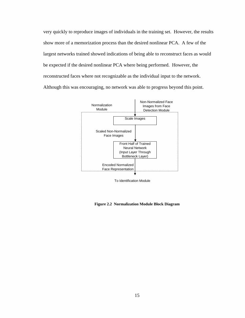
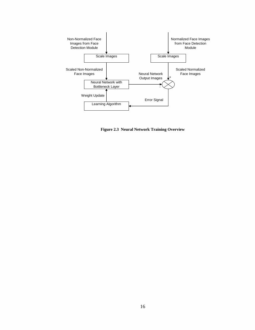
The normalization process is supposed to facilitate the recognition process by

eliminating factors in the image not related to the person’s identity. Ideally, the

normalization process would remove variations do to lighting, pose, expression etc. The

normalization algorithm investigated in this study was based on a neural network being

able to learn to perform a nonlinear PCA type dimensional reduction of face images. The

25

network was expected to create a dimensionally reduced representation of a normalized

face when given a non-normalized input face. For this to be successful a neural network

with a bottleneck layer must be trained to produce a normalized image of an individual

when given a non-normalized image of that same individual. Furthermore, such a

network must demonstrate the ability to combine features and create a new face when

presented with an individual not in the training set.

Training such a network required picking a normalized image for each individual

and using this as a target when the network was presented with any image of this

individual. Creating such training sets involved three steps. First the faces were detected

using a program called FaceDetect. Then the desired images for a given training set were

selected using a Microsoft Access database. Finally a program named DisplayFaces was

used to create training sets for the neural network.

3.4.1 Face Detection to Create Training Sets

A reliable face detection algorithm was required to create usable training sets for

the neural network. As the face detection via color segmentation algorithm did not

perform adequately, the OpenCV library was used to create a face detection application.

The OpenCV library is an open source C library for computer vision. It has a face

detection algorithm based on a cascade of boosted classifiers using Haar like features

[OpenCV 2007]. The application FaceDetect steps through a list of images utilizing the

OpenCV library to detect faces in each image. It then creates a CSV (comma separated

values) file containing the location of each face detected. From the original CMU PIE

database images, only images where the persons was facing within 45 degrees of forward

26

where passed to the FaceDetect program. This results in about 23000 locations being

labeled as faces.

3.4.2 Image Selection for Training Sets

The CSV file created by FaceDetect was imported as a table in Microsoft Access.

Figure 3.7 shows the structure of this table. The face detection process produced

numerous false detections. These had to be removed for the proposed neural network

training. Rather than sort through all these images by hand, it was decided to remove

face locations based on deviation from means. Since the CMU PIE database contains

multiple images of each individual from each camera and these images where taken very

rapidly with the subject sitting still, the location of the face for any given individual and

camera should be close across multiple images. A query was created in Microsoft

Access to calculate the standard deviation in the location and size of the detected faces

for a given individual and camera. A second query was then used to eliminate detected

regions that where outside a given number of standard deviations. This allowed many of

the false detections to be removed from the training set. The results of this query where

then exported to a csv file.

FacLoc PKID Autonumber Primary Key File Text Complete File Name ID Text Individiuals ID Type Text Image Type Cam Text Camera Face number Detected Face Number x number Upper Lefthand Corner x y number Upper Lefthand Corner y w number Width h number Height

Figure 3.7 MS Access Table Structure

27

The csv file exported from MS Access contained the image file name, the ID of

the individual, the image type, the face number, two integers specifying the x and y

location of the upper left hand corner of the face, and two integers specifying the width

and height for each face in the set. This file was then read by a program named

DisplayFaces. This program allowed each image listed in the csv file to be viewed with a

box around the detected face. The detected faces could then be manually removed from

the training set by clicking the remove button. After removing all false detections the

DisplayFaces application crops and scales the detected faces and combines them into a

neural network training (nnt) set file. The format of this binary file is shown in

Figure 3.8.

NNT File Header

Number Images int Width of Each Image int Height of Each Image int

For Each Image Full Path and File Name String Grayscale Bit Values unsigned char

Figure 3.8 Neural Net Training File Format

3.4.3 Neural Network Design

The design of the neural network was based on the standard back propagation of

errors algorithm and was implemented as a c++ class. Figure 3.9 shows the major

features of the class and the two support classes NNRnd and Sample. The private

member structure of the NeuralNet class, Layer, is also shown. The NNRnd class simply

encapsulates the random number generator in visual c++ and provides methods to return

various ranges of random numbers. The Sample class provides simplified input and

output options to the neural network. It stores arrays of input and output pairs and can be

28

passed directly to the training and execution routines in the NeuralNet class. Appendix B

describes the testing of these classes and some samples that indicate the correctness of the

implementation.

29

NeuralNet Class NNRnd Class Private Attributes Private Static Attributes

Nlayers int RndNum Random (Object) layer array of Layer objects Public Static Member Functions Err double Char unsigned char Desc String Double double TrainIter int PlusMinusOne double sfi - scale factor double array sfo - scale factor double array … Sample Class

Public Member Functions Public Attributes

Execute Inp unsigned char array

GetTrainIter Outp unsigned char array

Train Description String Scale ID String LearnRate InpWidth int LearnRateAdjust InpHeight int RandWeight OutpWidth int Save OutpHeight int Load Public Member Functions

Private Member Functions Sample FeedForward CreateSample BackProp GetSample WeightUpdate SetDescription MSE SetSize SaveScale Randomize LoadScale PrintSample SaveLayers PrintPairs LoadLayers SaveWeights LoadWeights Layer Struct LoadInputs ID int LoadTarget NNodes int ScaleOutput Out double array ResetDeltas Targ double array sigmoid Err double array W double array Wsaved double array dW double array pdW double array LR double MR double

Figure 3.9 NeuralNet Class and Support Classes

30

Layer Struct

The Layer struct is a private member of the NeuralNet class. This structure

contains the pertinent information about a layer of the network. Basic information such

as the number of nodes in the layer, the most recent output of each of those nodes and the

weights from each node in the previous layer to each node in the current layer is stored in

this structure. This structure also stores information related to the learning process such

as the error gradient associated with each node, the current and previous delta associated

with each weight, and the learning and momentum rates for the layer. The weights stored

in Layer are from nodes in the previous layer to nodes in the current layer. Thus, the

input layer does not have any weights. Layer also stores target outputs for the output

layer. These are not used in the other layers.

NeuralNet Class

The NeuralNet class encapsulates the functionality for setting up the neural

network, scaling the input and output, training and executing the network, and saving and

loading the network. As shown in Figure 3.9, the NeuralNet class contains an array of

Layer’s. It also contains integers to indicate the number of layers in the network and the

number of training iterations performed. The first step in creating a neural network using

the NeuralNet class would be to call the constructor. After creating the NeuralNet object,

scale factors could be set using the Scale member function. The network is then ready to

train using one of the Train member functions. After training, one of the Execute

member functions can be used to validate the training process. The network can also be

saved to and loaded from disk using the Save & Load member functions.

31

NeuralNet Constructor

The NeuralNet constructor creates a network with random weights, given an array

of int’s indicating the number of nodes per layer. Thus, if an array of ints containing the

values {5, 3, 2, 1} was passed to NeuralNet, a neural network with 4 layers, 5 inputs and

1 output would be created. This network would have two internal layers with 3 and 2

nodes respectively. Internally, this is accomplished by calling the Create function which

initializes all memory necessary and sets all initial values.

Scaling Input and Output

Scaling the input and output of a neural network helps prevent saturation and is a

widely used technique to improve network performance. The Scale member function

simplifies this process by determining the appropriate scaling for each input and output

and applying this scaling as needed. To enable scaling, the user needs to call the Scale

member function. This function takes 4 arrays of double precision numbers. The first

two arrays are the same length as the number of input nodes and indicate the minimum

and maximum possible values of these inputs respectively. The second two arrays are the

same length as the number of output nodes and likewise indicate the expected minimum

and maximum range of each output. The Scale member function uses these arrays to

calculate a set of linear scaling factors for each input and output. A flag is then set

indicating scaling is in effect. Once this flag is set any inputs sent to the network are

scaled prior to applying them to the network. Also, any network outputs are scaled back

to the original range prior to returning them to the user.

32

Training

There are two overloaded member functions called Train which can be used to

train the neural network. The only difference in the two functions is the format of the

training and testing samples. One function requires an array of Sample objects for each

of the training and testing samples. The other requires an ArrayList object which contain

Sample objects for each of the training and testing samples. Both functions also require

an integer indicating the maximum number of training iterations to process. The Train

function starts by passing each Sample from the test set to the network and determining

the cumulative error on the test set. This error will later be used to determine if training

has improved the network and to save the weights that performed the best on the test set.

The training iterations proceed as follows:

For each Sample in the train set: Pass the Sample through the network. Back propagate the errors from the target output.

Update the network Weights if non-epoch training. Update the network Weights if epoch training. For each Sample in the test set:

Pass the Sample through the network. Cumulate the test error.

If the test error is less than the previous test error, then store the weights

After completing the prescribed number of training iterations, the weights that performed

the best on the test set are re-loaded and the network is saved to disk.

Execute Member Functions

There are 5 overloaded member functions named Execute. They each pass a

given input Sample or set of input Samples’ through the neural network to produce an

output. The first two overloads receive a set of inputs via an array and produce an array

33

containing the network output. These two do not require a target output and thus do not

return the error of the network. They also only work with one set of inputs and outputs

per call. The next 3 overloads of Execute do return the error of the network based on a

given target. These 3 overloads receive either an array of Sample objects or an ArrayList

containing Sample objects. They execute each sample in turn and return the cumulative

error over the entire sample set. For the error returned to have meaning, each Sample

object must contain the target output corresponding to its input array. The other

variations in the overloads pertains to where the network output is stored and if it

overwrites the target output with the actual network output.

Save and Load Member Functions

Finally, the Save and Load member functions can be used to save and load the

neural network to and from disk. These functions accept an open FileStream object. The

Save member function writes the number of training iterations, the number of layers, and

the number of nodes in each layer to the FileStream. It then writes all the scale factors

for the network and all the weights for each layer to the FileStream. The Load member

function reads this exact same information. The current NeuralNet object is then re-

created using this information. If the number of nodes in each layer or the number of

layers read from the FileStream differs from the original NeuralNet object, Load returns

False otherwise it returns True. However, in either case the current NeuralNet object is

adjusted to match what was read from the FileStream.

34

3.4.4 Training Console

A c++.net application named TrainingConsole was created to train various neural

network configurations on the previously created training sets. This application is a

console application rather than a windows forms application. The name of a

configuration file is passed to this application from the command line. The format of this

text file is shown in Figure 3.10. The splits file referenced is a comma separated values

(csv) file with each line containing an individuals ID and an integer representing which

set (train = 1, test = 2, or validation = 3) this individual belongs to. The TrainingConsole

uses the information in the configuration file to train the specified neural network on the

specified training images.

NNC Text File Line # Description

1 Training Set File Name (.nnt file) 2 Target Set File Name (.nnt file) 3 Splits File Name (.csv file) 4 Number Training Iterations per call

5 Network Configuration (1024_10_1024)

6 Input Image Width 7 Input Image Height 8 Output Image Width 9 Output Image Height

Figure 3.10 Neural Network Configuration (.nnc) File

The TrainingConsole application uses the splits file to divide the images in the

training file into three sets. The train set is used to update the weights of the neural

network via the back propagation algorithm. The test set is used as a stopping condition

for the training. The validation set is used to verify the success of the networks learning.

The splits file is used to associate each individual with one of these three sets. Each

individual in the training file has an entry associated with their ID in the splits file. This

35

entry specifies which set their images belong to. The three sets are stored in ArrayLists

of Sample objects.

After the images in the training file are divided into sets, TrainingConsole begins

the training process. The ArrayLists containing the train set and the test set are passed to

the Train member function of NeuralNet and the network is trained for the specified

number of iterations. Recall, this member function saves and reloads the weights that

performed the best on the test set during the training process. After the prescribed

number of training iterations, each of the train, test, and validation sets are passed to the

trained neural network. For each of these sets, the input images, target output images,

and neural network output images are written to files to be read by the application

ResultsViewer. A flag file is then read from the default output directory. This file is the

users’ only interaction with TrainingConsole while it is running. If the first character of

the flag file is anything other than a ‘d’ for ‘decrease’ or a ‘s’ for ‘stop’ the training

continues for another set of iterations. If the first character of the flag file is a ‘d’ for

‘decrease’ then the learning and momentum rates are decreased and the training

continued for the specified number of iterations. If the files first character is a ‘s’ for

‘stop’ then the training stops and the program saves the best network found so far.

3.4.5 Viewing the Results

The output from the TrainingConsole program was read into a Windows forms

application called ResultsViewer. This application displays the input, target output, and

neural network output images side by side so that comparisons can be made. This

program also converts the resulting comparison images into a bitmap that can be saved to

file.

36

3.4.6 Neural Network Training

Multiple feed forward neural networks where trained using the back propagation

of errors algorithm with a momentum factor in an auto-associative configuration. The

networks included a hidden layer with a small (less than the number of individuals in the

training set) number of nodes. This configuration is known to be capable of performing

the desired PCA [Turk 1991]. A training set was created that only included one face for

each individual. The face included was forward facing, normally illuminated, and with a

neutral expression. The 68 individuals in the CMU PIE database where divided into the

train set, the test set, and the validation set. The train set was used with the back

propagation algorithm to update weights. The test set was used as the early stopping

criteria to prevent overtraining. The validation set was used in the final comparison of

multiple networks. Multiple network configurations where then trained using epoch

learning. When this failed to produce the desired results, the learning algorithm was

changed so that weight update took place after each sample presentation. As the trained

networks where never able to learn the desired behavior on this simple training set, more

difficult training sets where never presented. However, many modifications as to the

individuals in each of the train, test, and validation set where attempted. Also, for

validation of the process, networks where trained using only a single individual.

37

4. EVALUATION AND RESULTS


Color segmentation was found to be insufficient to detect human faces in realistic

photographs. The method was deficient in three main areas. First, if the images had

background areas that where close to skin colors, large areas of the photo would be

selected as ‘skin’. In some cases the areas where so large that multiple faces would be

considered a single skin region. This is demonstrated in Figure 4.1. The image on the

left is the original image. The image on the right is the component map showing the

detected components. The middle image shows the effect of applying the component

map as a mask to the original image. The second obstacle to using color segmentation

for face detection was its susceptibility to variations in lighting color. In the case of the

CMU PIE database apparently the blue content of the flashbulbs used resulted in very

little skin being detected. Figure 4.2 shows an image from the CMU PIE database with

both natural lighting and a flash. In fact, in almost all of the CMU PIE images where a

flash was used very little skin was detected. The final issue with using color

segmentation to detect faces involves selecting discontinuity in the detected region.

Because of the inability of the color segmentation to detect skin pixels and only skin

pixels, the actual face region is often segmented into multiple regions as shown in

Figure 4.3. There is no reliable way to know when to combine these regions and when

these regions represent separate faces.

38

Figure 4.1 Multiple Faces in a Single Component

Figure 4.2 Lighting Effect on Skin Detection

Figure 4.3 Multiple Components per Face

39

4.2 Neural Network

4.2.1 Concept Test – Single Individual Training

A simple training set was used to verify the NeuralNet class and algorithms and to

show the plausibility of the method. In this case a neural network was trained to

reproduce a single individual. Figure 4.4 shows the train and test sets for this case. The

three columns of images represent the input image, the target image and the neural

network output image respectively. It is interesting that the simplest possible network

with the required number of inputs and outputs was capable of learning this mapping.

For a 32 x 32 bit input image, a network with 1024 input nodes, 1 hidden node, and 1024

output nodes (here after abbreviated 1024 x 1 x 1024) was capable of recreating the input

image at the output. It took less than 10,000 training iterations to learn this mapping.

This indicates that the algorithm developed is capable of learning to produce a face

image. It is also indicative of the correctness of the developed applications.

40

1024 x 1 x 1024 Train Set Test Set

Figure 4.4 Single Individual Train Set

4.2.2 Epoch Training

When epoch training was used networks quickly learned to create an ‘average’

face. This ‘average’ face was then the output for any input given. When a face from any

of the three sets (train, test, or validation) where input to the networks trained this way,

this same ‘average’ face was output from the network. After this discovery all further

training was without epoch weight update.

4.2.3 One Image of Each Individual

The next training set investigated involved one image of each individual. The

neutral image (forward facing, natural lighting, neutral expression) of each individual

41

was used as both input and target output. This set consists of 68 images and was divided

into train, test, and validation sets. After eliminating epoch training, multiple networks

where found that where capable of learning the individuals in the train set. Figure 4.5

shows portions of the train set and the non-train sets. Restrictions on the publication of

images in the CMU PIE database prevent the entire sets from being presented. The

results shown are typical of such a network. As is shown in Figure 4.5, these networks

did not perform very well on the test and validation (non-train) sets. On these sets the

network typically output an image of one of the individuals from the train set. To be

considered successfully performing the desired PCA type combining of faces a network

would have to demonstrate the ability to output a face recognizable as that of the person

input to the network when presented with a face not present in the training set.

Interestingly, it was observed that the number of individuals the network could learn was

roughly the same as the number of hidden nodes for networks with a single hidden layer.

Figure 4.6 shows the results of a 1024 x 5 x 1024 network trained on 9 individuals.

Notice there are only about 5 distinct faces output by the network. This indicates the

network was performing more of a memorization than a PCA type computation.

42

1024 x 25 x 1024 Train Set Non-Train Sets

Figure 4.5 Typical Trained Network Results

43

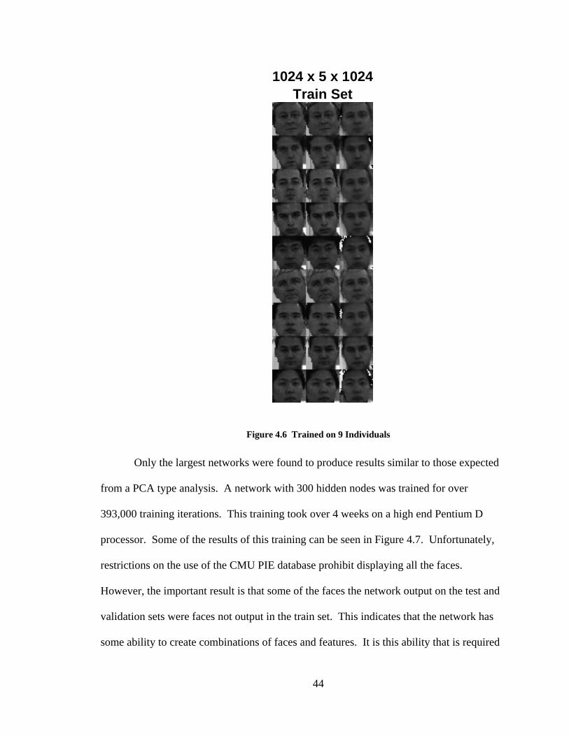
1024 x 5 x 1024 Train Set

Figure 4.6 Trained on 9 Individuals

Only the largest networks were found to produce results similar to those expected

from a PCA type analysis. A network with 300 hidden nodes was trained for over

393,000 training iterations. This training took over 4 weeks on a high end Pentium D

processor. Some of the results of this training can be seen in Figure 4.7. Unfortunately,

restrictions on the use of the CMU PIE database prohibit displaying all the faces.

However, the important result is that some of the faces the network output on the test and

validation sets were faces not output in the train set. This indicates that the network has

some ability to create combinations of faces and features. It is this ability that is required

44

for the network to be useful in the face recognition subsystem. However, the success of

this network was very limited. Although not apparent from Figure 4.7, the vast majority

of the faces output where unrecognizable. Even the faces that where indicative of the

ability to combine where not recognizable as the person input to the network.

1024 x 300 x 1024 Train Set Test Set Validation Set

Figure 4.7 Large Network Results

Three additional large networks where trained in the same manner as the 1024 x

300 x 1024. These networks included two additional hidden layers around the

bottleneck layer. According to [Bryliuk 2001] these additional layers should allow the

network to represent the nonlinear data with fewer “Principle Components”. Thus, the

bottleneck layer should not need to be as large. The three networks trained had 25 nodes

in the bottleneck layer. The additional hidden layers consisted of 100, 125, and 300

nodes. The resulting networks performed similar to the 1024 x 300 x 1024 shown in

Figure 4.7. Interestingly, the 1024 x 300 x 25 x 300 x 1024 network took less time to

train then the smaller 1024 x 300 x1024 network. This larger network converged in

about 30,000 training iterations.

45

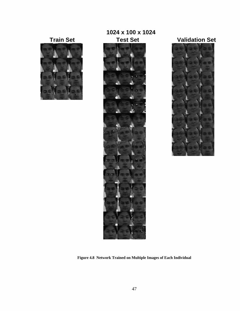
4.2.4 Multiple Images of Each Individual

The final training set used consisted of multiple images of each individual. The

forward facing, neutrally lit, talking, images from the CMU PIE dataset where used as

inputs. The target image for each individual was their neutral image. Networks trained

on this training set performed better than the large network trained above. Indications of

the ability to combine facial features where visible in the network output as shown in

Figure 4.8. However, the network output was still not recognizable as the person input.

In fact only a few of the output images demonstrated the desired combining of features.

Most of the images output on the test and validation sets where clearly the same image

output for an individual in the training set. For example, in the test set in Figure 4.8

consider the images of the two gentlemen with glasses in the eight and ninth row. The

network output the same face for each of these gentlemen and the same face was present

in the network output on the full training set.

46

1024 x 100 x 1024 Train Set Test Set Validation Set

Figure 4.8 Network Trained on Multiple Images of Each Individual

47

5. FUTURE WORK

5.1 Face Detection

Face detection via color segmentation seems to hold very little promise when

compared with the cascade of boosted classifiers using Haar like features method used in

OpenCV. The pitfalls of the color segmentation concept seem unlikely to be overcome

and thus do not warrant further investigation. However, the OpenCV method is far from

perfect and research into new face detection methods will need to continue if automated

face detection is to be reliable.

5.2 Neural Network Based PCA

Although the CMU PIE database had many images of each individual taken in

very well controlled conditions, the database only contains 68 individuals. Training on

similar images with more individuals may move the networks from a ‘memorization’

mode to a PCA type combination of facial features.

Future work should concentrate on larger neural networks, since the larger

network showed some promise in being able to perform a PCA type combination of

faces. However, the computational intensity of performing a thorough investigation

using large networks with a sufficiently large training set is daunting. Although Turk and

Pentland indicate a three layer network with a bottleneck layer is capable of performing

the desired PCA functions [Turk 1991] others suggest a five layer structure is better

suited for nonlinear data. Specifically, DeMers and Cottrell indicate that adding an

additional hidden layer on either side of the bottleneck hidden layer allows the network to

48

better represent nonlinear data with fewer “Principle Components”. They refer to the

additional layers as encoding and decoding layers [DeMers 1993]. Although a few

networks with five layers where trained, a more extensive search with a fuller dataset

may be productive. Likewise, improved training methods such as the variable learning

rates presented by Bryliuk and Starovoitov should be explored with a large face

dataset [Bryliuk 2001].

5.3 Additional Possible Focus Areas

In addition to the direct continuation of this work, several interesting concepts

were briefly explored which could be productive in this area. Many of these relate to the

discovery that neural networks in the proposed configuration where very good at

memorizing individuals. Although this ability did not directly fit with the proposed

system design, a system designed around this ability may prove productive. For example

a system could be designed were the end user actually trained a network on their

individual family. This network should be capable of identifying individuals it has been

trained on. Likewise, if a network is trained to reproduce a group of individuals and is

feed an individual not in the group, would the network output the person who looks the

most like the one input?

49

6. CONCLUSIONS

Despite the numerous applications for face detection and recognition, the current

methods are far from perfect. Thus, research will need to continue in this area if these

applications are to become commonplace. At this time a functioning face detection and

recognition subsystem suitable for a family photo album was not attainable using the

proposed system.


The color segmentation schemes investigated involved determining if each pixel

in a picture was ‘skin’ based on its color. Manipulations where then performed to group

these pixels for face detection. This method was very susceptible to color variations

caused by lighting, background, and skin color. It was found that other methods that

don’t rely on color where more capable of detecting faces in varying conditions.

6.2 Neural Network Based PCA

To be considered successfully performing the desired PCA type combining of

faces a network would have to demonstrate the ability to output a face recognizable as

that of the person input to the network when presented with a face not present in the

training set. If a neural network can be found which performs such a nonlinear PCA style

combining of faces and facial features it would be a very effective method of identifying

faces. The dimensionality reduction associated with this method would allow a

recognition module to work with a vector considerably smaller than the original image

size. This would considerably reduce the complexity of the recognition process. After

50

training multiple networks configurations on numerous images sets, no network was

found that adequately performed such a PCA combining of faces. However, there where

some networks that showed some indications of being able to perform such a combining.

These networks where not, however, able to recreate faces reliably enough to use as the

bases of a recognition module. Further study in this area should begin by using richer

training sets in an attempt to force the network to learn multiple individuals.

51

BIBLIOGRAPHY AND REFERENCES

[ACLU 2001] American Civil Liberties Union. ACLU Opposes Use of Face Recognition Software in Airports, Citing Ineffectiveness and Privacy Concerns (Oct. 2001). Available from http://www.aclu.org/Privacy/Privacy.cfm?ID=10263&c=130&Type=s (visited Feb. 26, 2005).

[ACLU 2003] American Civil Liberties Union. Three Cities Offer Latest Proof That Face Recognition Doesn’t Work, ACLU Says (Sept. 2003). Available from http://www.aclu.org/Privacy/Privacy.cfm?ID=13430&c=130 (visited Feb. 26, 2005).

[Basri 2001] Basri, R. and Jacobs, D. W. Lambertian Reflectance and Linear Subspaces. International Conference on Computer Vision, 2 (2001), 383-390.

[Belhumeur 1997] Belhumeur, P.N., Hespanha, J.P., and Kriegman, D.J. Eigenfaces vs. Fisherfaces: Recognition Using Class Specific Linear Projection. IEEE Trans. Pattern Anal. Mach. Intell. 19, 7 (1997), 711-720.

[Bryliuk 2001] Bryliuk, D. and Starovoitov, V. Application of Recirculation Neural Network and Principal Component Analysis for Face Recognition. The 2nd International Conference on Neural Networks and Artificial Intelligence, (October 2001), 136-142.

[DeMers 1993] DeMers, G. and Cottrell, G. Nonlinear Dimensionality Reduction. Advances in Neural Information Processing Systems 5, (1993), 580-587.

[Digitalcamerainfo 2005] Fujifilm Displays Face Recognition and Detection Ability; Available in new Electronic Photo Album. Available from http://www.digitalcamerainfo.com/content/Fujifilm-Displays-Face-Recognition-and-Detection-Ability-Available-in-new-Electronic-Photo-Book.htm (visited Feb. 24, 2005).

[Er 2002] Er, M.J., Wu, S., Lu, J., and Toh, H.L Face Recognition with Radial Basis Function (RBF) Neural networks. IEEE Transactions on Neural Networks, 13, 3 (May 2002), 697-710.

[Fisher 1994] Fisher, B., Perkins, S., Walker, A., and Wolfart, E. Department of Artificial Intelligence University of Edinburgh UK. Hypermedia Image Processing Reference (1994). Available from http://www.cee.hw.ac.uk/hipr/html/histeq.html (visited Mar. 30, 2005).

[Frischholz 2005] Frischholz, R.W. Face Detection Home Page. Techniques. Available from http://home.t-

52

online.de/home/Robert.Frischholz/facedetection/techniques.htm (visited Mar. 1, 2005).

[Georghiades 2001] Georghiades, A., Belhumeur,P., and Kriegman, D. From Few to Many: Illumination Cone Models for Face Recognition under Variable Lighting and Pose. IEEE Trans. Pattern Anal. Mach. Intelligence, 3, 21 (June 2001), 643-660.

[Jebara 1996] Jebara. T.S. 3D Pose Estimation and Normalization for Face Recognition. Undergraduate Thesis, Center for Intelligent Machines, McGill University (May 1996). Avaible from http://www1.cs.columbia.edu/~jebara/papers.html (visited Mar. 30, 2005).

[Jung 2002] Jung, D.J., Lee, C.W., Lee, Y.C., Bak, S.Y., Kim, J.B., Kang, H., and Kim, H.J., Proceedings International Technical Conference on Circuits/Systems, Computers and Communications (Jul. 2002), 615-618.

[Lawson 2005] Lawson, E. Summary: ”Eigenfaces for Recognition” (M. Turk, A. Pentland). Available from http://cs.gmu.edu/~kosecka/cs803/Eigenfaces.pdf (visited Mar 06, 2005).

[Moses 1994] Moses, Y., Adini, Y., and Ullman, S. Face recognition: The problem of compensating for changes in illumination direction. European Conference on Computer Vision, (1994), 286-296.

[Murase 1995] Murase, H., and Nayar, S. Visual Learning and Recongintion of 3D object from appearance. International Journal of Computer Vision, 14, 1 (1995), 5-24.

[OpenCV 2007] OpenCV Library Wiki. Face detection using OpenCV page. Available from http://opencvlibrary.sourceforge.net/FaceDetection (Visited Mar. 8, 2007).

[Orr 1999] Orr, G., Schraudolph, N., and Cummins, F. Willamette University Professor Genevieve Orr Home page. CS-449: Neural Networks (Fall 1999). Available from http://www.willamette.edu/~gorr/classes/cs449/intro.html (visitied April 19, 2005).

[Rowley 1998] Rowley, H.A., Baluja, S., and Kanade, T. Neural Network-Based Face Detection. IEEE Transactions on Pattern Analysis and Machine Intelligence, 20, 1 (Jan 1998), 23-38.

[Seshadrinathan 2003] Seshadrinathan, M., and Ben-Arie, J. Face Detection by Integration of Evidence. IASTED International Conference on Circuits, Signals and Systems, (May 2003), 241 -246.

[Shan 2003] Shan, S., Gao, W., Cao, B., and Zhao, D. Illumination Normalization for Robust Face Recognition Against Varying Lighting Conditions. IEEE International Workshop on Analysis and Modeling of Faces and Gestures, (2003), 157-164.

53

[Shashua 1997] Shashua, A., On Photometric Issues in 3D Visual Recognition from a Single 2D Image. International Journal of Computer Vision (IJCV), (1997), 99-122.

[Shashua 2001] Shashua, A., and Riklin-Raviv, T., The Quotient Image: Class-Based Re-Rendering And Recognition With Varying Illuminations, IEEE Trans. On PAMI, 23, 2 (2001), 129-139.

[Sim 2002] Sim, T., Baker, S., and Bsat, M., The CMU Pose, Illumination, and Expression (PIE) Database. Proceedings of the 5th International Conference on Automatic Face and Gesture Recognition, (2002), 53-58.

[Storring 1999] Storring, M., Andersen, H.J., and Gramum, E. Skin colour detection under changing lighting condititions. 7th Symposium on Intelligent Robotics Systems, (July 1999), 20-23.

[Turk 1991] Turk, M., and Pentland, A. Eigenfaces for Recognition. Journal of Cognitive Neuroscience, 3, 1 (1991), 71-86.

[Vezhnevets 2003] Vezhnevets V., Sazonov V., and Andreeva A. A Survey on Pixel-Based Skin Color Detection Techniques. Proc. Graphicon, (Sept. 2003), 85-92.

[Viisage 2004] Viisage in the Media. Face recognition finds its identity (July 2004). Available from http://www.viisage.com/en/data/pdf/en_2004-07_id-world_face-recognition.pdf (visitied Feb. 26, 2005).

[Wikipedia 2007] Wikipedia, the Free Encyclopedia. OpenCV - Wikipedia page. Available from http://en.wikipedia.org/wiki/Opencv (Visitied Feb. 27, 2007).

[Yang 1996] Yang, J., and Waibel, A. A Real-Time Face Tracker. Third IEEE Workshop on Applications of Computer Vision, (1996), 142-147.

[Yang 2002] Yang, M.H., Kriegman, D.J., and Ahuja, N. Detecting Faces in Images: A Survey. IEEE Transactions on Pattern Analysis and Machine Intelligence, 24, 1 (Jan 2002), 34-58.

[Yang 2004] Yang, M.H. Recent Advances in Face Detection, IEEE International Conference on Pattern Recognition 2004 Tutorial, (2004).

[Zhao 2000] Zhao W.Y., and Chellappa, R. SFS Based View Synthesis for Robust Face Recognition. Proc. 4th Conference on Automatic Face and Gesture Recognition, (2000), 285-292.

[Zhao 2003] Zhao, W., Chellappa, R., Phillips, P.J., and Rosenfeld, A. Face Recognition: A Literature Survey. ACM Computing Surveys, 35, 4 (Dec. 2003), 399-458.

54

APPENDIX A – TERMS

Facial Image Features [Yang 2004]

Pose (Out-of-Plane Rotation): frontal, 45 degree, profile, upside down.

Structural components: beards, mustaches, and glasses.

Facial expression: face appearance is directly affected by a person's facial expression.

Occlusion: faces may be partially occluded by other objects.

Orientation (In-Plane Rotation): face appearance directly vary for different rotations

about the camera's optical axis.

Imaging conditions: lighting (spectra, source distribution and intensity) and camera

characteristics (sensor response, gain control, lenses), and resolution.

Face Detection Algorithm Categories [Yang 2002]

Knowledge-based methods: These rule-based methods encode human knowledge of what

constitutes a typical face. Usually, the rules capture the relationships between

facial features. These methods are designed mainly for face localization.

Feature invariant approaches: These algorithms aim to find structural features that exist

even when the pose, viewpoint, or lighting conditions vary, and then use the these

to locate faces. These methods are designed mainly for face localization.

Template matching methods: Several standard patterns of a face are stored to describe the

face as a whole or the facial features separately. The correlations between an input

image and the stored patterns are computed for detection. These methods have

been used for both face localization and detection.

55

Appearance-based methods: In contrast to template matching, the models (or templates)

are learned from a set of training images which should capture the representative

variability of facial appearance. These learned models are then used for detection.

These methods are designed mainly for face detection.

56

APPENDIX B – CORRECTNESS OF NEURAL NETWORK CODE

The correctness of the neural network code was tested using both black box and

white box testing methods. In addition, all subroutines and member functions where

tested individually prior to being included in the complete algorithm. After verification

of the implementation of the algorithms, numerous feasibility test where performed to

verify the use of the neural network in a PCA configuration.

White Box Testing

White box testing focused mainly on the neural network computations. Since

these computations are extensive, it was felt necessary to perform the computations by

hand and verify the correctness of the algorithm. In order to accomplish this, a few very

small networks where given inputs, target outputs, and set weights. Both the feed

forward computations and the back propagation of errors computations where performed

by hand and compared to the network. The various values associated with each node in

the network where compared with those computed by hand. It was determined that the

network computations where correct.

Black Box Testing

Black box testing consisted of training the neural network on numerous test cases

to verify its ability to learn. The objective of this testing was to verify the functionality of

the entire neural network class (NeuralNet) and its associated classes. These test where

designed specifically to demonstrate errors that could not easily be demonstrated by hand

calculations. These test where also used to verify the member functions such as input,

57

output, scaling, saving, loading, and initialization functions that are not directly related to

the numeric computations.

Black Box Testing Examples

A few of the numerous test cases used to verify the neural network code are

presented here. The first case is a simple sinusoidal function. The input and output

where scaled and converted to single byte char values. This test verifies the NeuralNet

classes i/o routines when presented with single byte char data. As can be seen in

Figure B.1 the small 1-3-1 network does a reasonable job of learning the sine function. A

larger network (1-5-1) is trained on a more complex sinusoidal function in Figure B.2.

This test demonstrates the networks ability to learn.

58

Sine Test 1-3-1 Network

0

50

100

150

200

250

300

0 50 100 150 200 250 300

X as Single Byte Char

Y as

Sin

gle

Byt

e C

har

Sine FunctionNeural Network

e

Figure B.1 NeuralNet Test - Sin

59

Complex Sinusoidal Function 1-5-1 Network

0

50

100

150

200

250

300

0 50 100 150 200 250 300

X as Single Byte Char

Y as

Sin

gle

Byt

e C

har

Sinusoidal FunctionNeural Network

PCA Configur

The nex

configuration l

same and the n

hidden layer w

successfully us

successfully re

described below

The firs

Random x valu

Figure B.2 NeuralNet Test – Complex Sinusoidal Function

ation Verification

t set of test performed sought to verify the use of the neural network in a

ike that used for PCA. Namely, the inputs and the target outputs are the

etwork is structured with a bottleneck layer. A bottleneck layer is a

ith fewer nodes that the number of inputs. For the network to be

ed to perform a PCA like dimensional reduction, the network must

produce the inputs at the outputs. Some of the testing examples used are

.

t PCA test involved two simple linear functions, y0 = x and y1 = -x.

es between -1 and 1 where used to calculate these two inputs. A 2-1-2

60

network was trained to reproduce the input at the output. Figure B.3 shows the results of

this test. This case is somewhat trivial because one of the inputs is the principle

component the network is expected to utilize.

Simple Linear PCA with 2-1-2 Neural Network

0

50

100

150

200

250

300

0 50 100 150 200 250 300

x as Single Byte Char

y as

Sin

gle

Byt

e C

har

y0 = x NN - y0

y1 = -x NN - y1

s

Figure B.3 PCA Test with Simple Linear Function

61

The second PCA test was designed such that the principle component the

functions where based on was not included in the input set. In this test y0 = x*x and

y1 = 1.5*x*x – x + 0.5. Again, this test is very similar to the first test, however, the

principle component x is not passed as an input to the network. The smallest network

found to be capable of learning this mapping was a 2-2-1-2-2 network. Figure B.4 shows

the output of this network.

Quadratic with 2-2-1-2-2 Neural Network

-50

0

50

100

150

200

250

300

-0.2 0 0.2 0.4 0.6 0.8 1 1.2

x

y as

Sin

gle

Byt

e C

har

y0 = x*x NN - y0

y1 = 1.5*x*x - x + 0.5 NN - y1

Figure B.4 PCA Test with Quadratic Functions

62

Date post:	29-Apr-2018
Category:	Documents
Upload:	dangphuc
View:	214 times
Download:	1 times

ABSTRACT - Texas A&M University–Corpus Christisci.tamucc.edu/~cams/projects/293.pdfEVALUATION AND...

Documents