ABSTRACT Title of Thesis: THE INFLUENCE OF LAND-USE, ENVIRONMENT, AND SOCIOECONOMIC FACTORS ON TREE SPECIES DISTRIBUTION IN BALTIMORE, MARYLAND. Degree Candidate: Kimberley Ellen Mead Master of Science, 2009 Directed By: Associate Professor Joseph H. Sullivan Department of Plant Science and Landscape Architecture With the exponential growth in human population and rapid increase in global urbanization, understanding changes in community dynamics and structure in human dominated landscapes is essential, yet, rarely studied. To determine what factors account for tree species composition and distribution in an urban setting, data from the 1999 UFORE Model vegetation survey of Baltimore, Maryland was analyzed. There was a diverse arboreal population found, comprised primarily of species native to the area. Detrended correspondence analysis did not show a clear pattern of species assemblages based on land-use, possibly indicating a homogenization of conditions across the urban environment. In canonical correspondence analyses,
Transcript
ABSTRACT
Title of Thesis: THE INFLUENCE OF LAND-USE,
ENVIRONMENT, AND SOCIOECONOMIC FACTORS ON TREE SPECIES DISTRIBUTION IN BALTIMORE, MARYLAND.
Degree Candidate: Kimberley Ellen Mead
Master of Science, 2009 Directed By: Associate Professor Joseph H. Sullivan
Department of Plant Science and Landscape Architecture
With the exponential growth in human population and rapid increase in global
urbanization, understanding changes in community dynamics and structure in human
dominated landscapes is essential, yet, rarely studied. To determine what factors
account for tree species composition and distribution in an urban setting, data from
the 1999 UFORE Model vegetation survey of Baltimore, Maryland was analyzed.
There was a diverse arboreal population found, comprised primarily of species native
to the area. Detrended correspondence analysis did not show a clear pattern of
species assemblages based on land-use, possibly indicating a homogenization of
conditions across the urban environment. In canonical correspondence analyses,
species distribution could not be explained by socioeconomic factors, however, there
was a significant relationship of tree species assemblages and the physical
environment, specifically with percent impervious surface cover. The amount of
variance accounted for was small indicating that other factors may be involved in
determining plant species assemblages.
THE INFLUENCE OF LAND-USE, ENVIRONMENT, AND SOCIOECONOMIC FACTORS ON TREE SPECIES DISTRIBUTION IN BALTIMORE, MARYLAND.
By
Kimberley Ellen Mead
Thesis submitted to the Faculty of the Graduate School of the University of Maryland, College Park, in partial fulfillment
of the requirements for the degree of Master of Science
2009
Advisory Committee: Associate Professor Joseph H. Sullivan, Chair Research Forester, United States Forest Service, Richard V. Pouyat Associate Professor David Meyers
I would like to thank my advisor, Dr. Joseph H. Sullivan, and my thesis committee member, Richard Pouyat, for not only their helpful comments and time, but more
importantly, for their steadfast support and endless patience. Thank you to Dr. Maile Neel for setting a remarkable standard for what a woman can accomplish in the
scientific world. And to Dr. David Myers for stepping in at the last minute without hesitation.
I would like to thank my family for all of their encouragement. I have been blessed
with eternally loving and supportive parents who never lost faith and, who, no matter the outcome, I could never disappoint. Thank you to my roommate and soul sister, Elisabeth, for all of her cheerleading and wine reserves. To my brother, Shawn, for skeeball, bad movies, and homemade pizza. And to Nathan, who captured my heart,
and continues to challenge me to discover new things about myself.
I would like to express my appreciation to all of my friends for always seeking new adventures and keeping me young at heart. And to my fellow graduate students, for their fellowship, their positive criticisms, and for inspiring me with their brilliance.
iii
Table of Contents Acknowledgements....................................................................................................... ii List of Tables ............................................................................................................... iv List of Figures............................................................................................................... v Chapter 1: Introduction................................................................................................. 1
The challenges for urban vegetation ......................................................................... 2 Socioeconomic factors versus abiotic and biotic factors in determining plant composition and diversity ......................................................................................... 5 Questions and hypotheses ......................................................................................... 7
Chapter 2: Methods....................................................................................................... 9 Site description – Baltimore, MD ............................................................................. 9 Description of the Urban Forest Effects Model (UFORE) ..................................... 11 Survey design and plot selection............................................................................. 12 Vegetation data collection....................................................................................... 14 Data analysis: Importance values and species diversity ......................................... 16 Data analysis: Detrended correspondence analysis ................................................ 17 Data analysis: Canonical correspondence analysis relating census information .... 19
Chapter 3: Results....................................................................................................... 22 The genera and species composition of trees found in the Baltimore City survey. 22 Tree species prevalence .......................................................................................... 24 Tree species origins................................................................................................. 29 Tree species frequency............................................................................................ 31 Land-use classifications of the plots ....................................................................... 34 Tree species diversity within land-use classifications ............................................ 35 Detrended correspondence analysis of tree species across land-uses..................... 41 The relationship between socioeconomic variables and tree species composition. 45 The relationship between anthropogenic environmental variables and tree species composition............................................................................................................. 51 The impact of soil properties on tree species compositions ................................... 56
Chapter 4: Discussion ................................................................................................. 58 The history of dominant trees in Baltimore ............................................................ 58 Trees in Baltimore today......................................................................................... 59 Invasive species in Baltimore ................................................................................. 66 Tree species and groundcover by land-use ............................................................. 70 Detrended correspondence analysis of species distribution related to land-use ..... 78 The analysis of socioeconomic and environmental variables through canonical correspondence analysis.......................................................................................... 83 Conclusion .............................................................................................................. 91
Appendix 1: Species Codes ........................................................................................ 94 Appendix 2: Species by land-use................................................................................ 96 Bibliography ............................................................................................................. 100
iv
List of Tables
1. Tree species found, diversity indices, and importance values…………25-26.
2. Widely distributed tree species.…………………………..…….……..….33.
3. UFORE land-use classes and the number of plots in each………………34.
4. Most common tree species by land-use…………………………………..36.
5. Diversity indices by land-use……………………………………………..40.
6. Census information used in canonical correspondence analysis……….…45.
7. Canonical coefficients and correlations of socioeconomic factors…….…48.
8. Average percent impervious surface for each land-use…………………...52.
9. Axis summary statistics for CCA of environmental factors...………...….54.
10. Canonical coefficients and correlations of environmental factors…….….55.
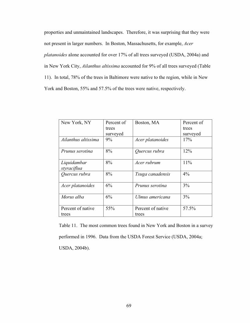
11. Comparative data: Most common trees found in New York and Boston…69.
v
List of Figures
1. Relative proportions of genera surveyed………………………………….23.
2. Proportions of native, exotic and invasive trees…………………………..30.
3. Proportion of tree species considered invasive……………………………31.
4. Detrended correspondence analysis of tree species by land-use………….42.
5. Map of Baltimore City’s census tracts……………………………………44.
6. Canonical correspondence analysis biplot of socioeconomic data…….…47.
7. Canonical correspondence analysis biplot of socioeconomic data with
only residential plots……………………………………………………...50.
8. Canonical correspondence analysis biplot of median age of structure
and plot percent impervious cover……..…………………………………53.
9. Canonical correspondence analysis biplot of USDA Forest Service
soil data for select Forest plots……………………………………………57.
vi
List of Illustrations
1. Map of Baltimore City UFORE plots…………………………………….10.
1
Chapter 1: Introduction
Few ecosystems are untouched by the direct and subtle effects caused by the
development and expansion of human civilization (McDonnell and Pickett, 1993). In
the United States, approximately 80% of the population lives in or near cities
(USCB, 2005), while the surface area of urban areas is projected to almost double in
the next 25 years to 9.2% (Alig et al., 2004). Worldwide, an estimated five billion
people will be living in urban areas by the year 2030 (UN, 2005). Despite the
increase in urban population, little research in North America has focused on
understanding the community dynamics of city-dwelling plant species or ecosystem
functioning within urban environments (Collins et al., 2000). In large part, this lack
of attention stems from the fact that forests dominated by humans and urban
infrastructure are rarely seen as functioning ecosystems by citizens and scientists
alike as vegetation is forced to exist within disconnected forest remnants, street tree
pits, and highly variable residential and commercial landscapes. In order for planners
and both public and private land stewards to make informed decisions that will
protect and improve environmental and, ultimately, human health and well-being,
there must be a greater understanding of how human dominated systems function
(Meiners et al., 2001).
2
The challenges for urban vegetation
Urban environments differ in many respects from more researched and
understood rural and wilderness settings. Urban areas are defined here as areas
containing more than 620 people per km2 with an overall population greater than
50,000 (USCB, 1980). Typically, population density, the proportion of land
apportioned to buildings, and road density are all highest near the urban core and
decrease with distance outwards as the forest matrix becomes more dominant
(Medley et al., 1995). Cities are often characterized by a low percentage of forested
area (Medley et. al, 1995) with an average of 33% tree cover for cities in the northeast
United States (Nowak and Crane, 2002) compared with surrounding rural areas
characterized by about 80% tree cover, on average (Freedman et al., 1996). Land that
is available for tree growth is broken into more numerous and smaller isolated
fragments (Medley et al., 1995; Porter et al., 2001), reducing available space for the
establishment and persistence of species adapted to the protection provided for by the
forest interior.
In more natural forested areas, disturbance events include fire outbreaks and
tree falls (Pickett et al., 1989). While in an urban environment, disturbance is
commonly a result of land-use change and new construction. Practices in land
management, such as lawn mowing, can provide for more frequent, smaller scale
disturbances. However, while the actual pathways may be markedly different, urban
forests and rural forests are similar in the mechanisms of vegetation community
dynamics. As in forest species assemblages found in more rural settings, trees in
urban forests are distributed based on generalized mechanisms of species
3
replacement: 1) sites become available, 2) species are differentially available based
on seed source or vegetative propagation, and 3) species are able to persist through
adaptation and competition (Pickett et al., 1987).
Once space is available for tree growth, the species available to regenerate
naturally are determined by the available seed source and by adjacent species able to
vegetatively propagate and colonize the area. In cases where trees are being planted,
species composition is in large part due to the availability of plant material, trends in
landscaping, and personal preference. Only those native trees able to adapt to the
transition from undisturbed forest to developed city will persist and regenerate in
natural areas as well as spread into neglected and abandoned private land spaces.
Species composition and distribution in the urban environment can also differ
when compared with surrounding areas due to the introduction of non-native species.
Non-native species are defined as those species that were not found in the Baltimore
area pre-European settlement and have since then been imported from areas of similar
climatic characteristics, mainly portions of Asia and Europe, for landscaping,
medicinal purposes and soil erosion control. Some of these non-native species may
naturalize through environmental adaption and freely reproduce while others do not
escape into the environment. Invasive species are those non-native species that
aggressively spread and are found to cause economic and environmental harm or
harm to human health (Swearingen, 2002).
There is often a larger stem densities of non-native plant species around
developed areas that increases overall species richness (Burton and Samuelson, 2008;
Lowenstein and Lowenstein, 2005; Sax and Gaines, 2003) and leads to biotic
4
homogenization at small, large, and global spatial scales as cities are built to serve a
single species, man (McKinney, 2006). Forests along an urban-rural gradient in New
York were found to have lower stem densities and an increased proportion of invasive
seedlings and saplings, as well as seed bank stores, at the urban end of the gradient
(Cadenasso et al., 2007, McDonnell et al, 1997). Previous studies have shown that
native plant communities in urban areas typically have decreased stem densities,
lower species diversity, and decreasing overstory tree regeneration (Burton and
Samuelson, 2008, Moffatt et al., 2004). Species composition in cities can be
dominated by few species accounting for more than half of the tree population
(Nowak, 1994d).
Finally, after a tree seed germinates, it has to be able to persist in that
location. With the intensive construction and constant modification needed to support
a large human population, urban areas are characterized by conditions challenging to
some species of trees such as altered hydrology (Groffman et al., 2003) and a higher
percentage of impervious groundcover affecting water flow and plant root growth
(Medley et al., 1995). Soils are typically compacted and degraded with altered
nutrient cycling (Groffman et al., 1995; Pickett et al., 1997), higher concentrations of
heavy metals and organic matter, and reduced fungi and microinvertebrates
(McDonnell et al., 1997; Pouyat et al., 1995). Urban areas are prone to the “heat
island effect” where anthropogenic changes to land cover and pollution have resulted
in temperatures higher than surrounding rural areas (Karl et al., 1988; Oke, 1995),
possibly leading to longer growing seasons and altered flowering times for resident
plant species (Luo et al., 2007). These factors, along with many others, including the
5
unique history and development of each patch of land, may influence the plant
species assemblages found within the urban environment.
Socioeconomic factors versus abiotic and biotic factors in determining plant composition and diversity
Urbanization has resulted in new definitions for plant community ecology and
new parameters for species composition and spatial relationships. In natural systems,
site characteristics such as climate, resource availability, hydrology, seed source
proximity and dispersal, and topography are typically the dominant factors in
determining species composition and spatial distribution (Brush, 1980; Chesson,
2000; Grimes, 1979; Lavorel, 2002). However, in an environment modified by and
dominated by humans, abiotic and biotic factors become integrated, or sometimes
replaced, with site history, socioeconomic status, cultural influences, and personal
preferences.
Hope et al. (2003) found in planted landscapes that perennial plant diversity in
urban gardens was affected by the “luxury effect”, the relationship of wealth and
plant diversity, in addition to elevation and land-use (Hope et al, 2003). Martin et al.
(2004) investigated the sources of variation in perennial vegetation composition
planted across the landscape of Phoenix, Arizona. Median family income accounted
for most of the variation in plant richness in neighborhoods. Plant abundance in
surrounding park land was best predicted by the time since last disturbance
represented by the median age of the neighborhood.
6
Grove et al. (2006) investigated the importance of multidimensional social
theories on vegetation cover in Baltimore, Maryland by extracting land cover from
satellite imagery in terms of grass cover versus tree cover on residential areas located
on private lands, public rights-of-way, and riparian areas. They found that tree
canopy cover, on private lands and on public rights-of-way, was best predicted by the
land management decisions aimed towards upholding prestige within the community,
particularly when modeled with housing age.
While there have been some gains in the understanding of the interaction of
humans and vegetation in urban environments, little has been investigated within
urban areas on arboreal vegetation at the species level. Whitney and Adams (1980)
found that age of housing on the property and the proximity to the center of Akron,
Ohio greatly influenced the tree species present. They suggested that this may have
been due to the changing recommendations by the nursery industry as plants go in
and out of fashion over time. Plants in more developed areas closer to the city’s
central complex were more likely to be undesirable species, such as Morus alba and
Ailanthus altissima, due to differential property upkeep, if any at all, as land
management can be absent with vacant property in comparison to suburban areas.
They also found correlates in income and occupation of the homeowner. Vallet et al.
(2008) found that buildings and pavement areas were significant predictors of species
composition.
In an effort to further research the drivers for tree species assemblages in an
urban environment, tree survey data was collected and used in a series of multivariate
7
analyses in order to evaluate chosen social and environmental factors found in
previous studies to influence vegetation distribution.
Questions and hypotheses
Using data collected from a vegetation survey from the UFORE Model
collected in Baltimore, Maryland in 1999 by the USDA Forest Service, the following
analyses will attempt to describe the tree populations found, as well as the possible
drivers for tree species composition, and their positioning in the urban landscape.
UFORE, or the Urban Forest Effects Model, is a computer model developed in the
1990’s by the USDA Forest Service Northeastern Research Station to quantify an
urban forest’s structure and function (Nowak and Crane, 2000).
Survey plots were grouped by land-use type as this can be an indicator of site
history, degree of disturbance, and of land management practices. In this study, three
questions will be addressed. What is the current tree population of Baltimore, MD
and does land-use influence the spatial distribution of tree species? And finally, as
the natural environment is heavily modified, do anthropogenic processes act as
drivers for tree species composition and distribution? The following hypotheses will
be tested with the purpose of answering these questions:
(H1) Differences in species assemblages among the survey plots will be
related to land-use classification.
8
(H2) Socioeconomic data, specifically income, population density, and percent
vacant housing, will be correlated with tree species distribution.
(H3) Physical environmental data, represented by impervious surface cover
and time since last major disturbance, will be significant to tree species
distribution.
9
Chapter 2: Methods
Site description – Baltimore, MD
All plots surveyed were within the city limits of Baltimore, Maryland, located
in the Mid-Atlantic region of the United States (Illustration 1). Baltimore City (lower
left 39˚11’37” N, 76˚42’38” W and upper right 39˚22’30” N, 76˚31’42” W) is located
on the Patapsco River, which empties into the Chesapeake Bay. The city is protected
to the west by the Appalachian Mountain range, blocking northern winds and lake
effect snows from the Great Lakes region. To the east, the Atlantic Ocean buffers the
area from extreme freezing conditions. The average annual rainfall is 100-115
centimeters and is generally distributed evenly throughout the year with around 10
centimeters per month with the exception of late spring and early summer where there
is a slight increase in precipitation (NOAA, 2004). The highest daily temperatures
typically occur in July at an average of 32.8˚ C and lowest temperatures take place in
January with an average low of 6.7˚ C. The record high was 42˚ C in 1985 and the
record low was set in 1934 at -21.7˚ C (TWC, 2007). Primarily located within Plant
Hardiness Zone 8, a small portion of zone 7 occupies the north-western part of the
city according to the USDA Hardiness Zone map (USDA, 1990). The fall line,
designating the meeting of two physiographic regions, the Atlantic Coastal Plain and
the Piedmont, cuts through the city, nearly dividing Baltimore into half. The city’s
elevation ranges from sea level to 400 feet above sea level with the center of the city
about 33 feet above sea level (USGS, 2008).
10
Illustration 1. A map of Baltimore City with the 1999
UFORE plots marked and land-use categories indicated
(Courtesy of the USDA Forest Service; Pouyat et al., 2007).
11
Baltimore’s population peaked in the 1950’s as the sixth largest city in the
United States and then began to decline as people moved into the surrounding
suburbs. The population in 2000 was estimated to be 651,154 people by the United
States Census Bureau, down 14.7% from 1990’s estimate of 763,014. Although still
falling, the population decline has slowed in recent years to 631,366 in 2006. City
revitalization projects including the renovation of the Inner Harbor, a popular tourist
attraction, and increased residential building may have contributed to the reduced rate
of population decline. Even with the recent renewal, a large percentage of the
population lives below the poverty line with an unemployment rate of 22.9% and
much of the city’s landscape is abandoned and unattended with a vacant housing
estimate of 42,000 homes (Chapelle et al., 1986; US Census, 2008).
Description of the Urban Forest Effects Model (UFORE)
Data for this analysis have been provided by the USDA Forest Service from a
vegetation survey in the summer of 1999 (UFORE, 2004c). The UFORE computer
model was developed in the 1990’s by the United States Department of Agriculture
Forest Service, Northern Research Station to allow researchers and land managers to
quantify the structure, functions, and values of forests using vegetation data collected
in the field and corresponding meteorological and pollution data (Nowak and Crane,
2000). The program began with a handful of large cities within the United States,
such as New York, NY, Atlanta, GA and Baltimore, MD and has since been utilized
in approximately 50 cities throughout the world. The UFORE model can provide
information as to the current state of a city’s forest and management opportunities
12
through species diversity, forest health, and age class distribution. In addition, the
model has been used to predict the future health of the city’s forest and to provide
political ammunition and perhaps a will to enact policies that will preserve and
improve a forest’s current state. The model calculates a monetary valuation of an
urban forest, the potential losses due to invasive trees, pests, and pathogens, and the
environmental services provided by the city’s forest including building temperature
moderation and air pollution uptake (Nowak and Crane, 2002).
Survey design and plot selection
Urban landscapes are collections of patches of the landscape that differ
physically, biologically, and socially. Research has suggested that, in urban
landscapes, topography and climatic variables are overcome by anthropogenic factors
and spatial connectivity when determining species presence (Guirado et al., 2008). In
a city, land-use has an overall impact on the amount of tree cover (Nowak et al.,
2002). Industrial sites, for example, can be predicted to have a smaller percentage of
tree cover, a higher percentage of impervious groundcover, and to have greater
degrees of environmental disturbance than other types of land-uses. In contrast,
canopied forested sites can be expected to have little, if any, impervious groundcover,
less disturbance, and higher tree stem density and species diversity than industrial
sites and other highly developed land-uses. Therefore, these patches, if grouped by
current overall land-use of the surveyed area, are more easily defined and studied, as
well as potentially better managed for optimum tree health and survivability. With
13
this in mind, experimental design of the UFORE vegetation analysis uses a land-use
typology to stratify plot locations.
As part of the UFORE data collection process, 202 circular 1/10 acre stratified
random plots were selected in 1999 within the city limits of Baltimore, Maryland. A
map representing a modified Anderson Level II classification was entered into a
UFORE random plot selection program developed by the US Forest Service as a tool
in ArcGIS (ESRI, 2006). The number of plots in each land-use category was based
on the relative proportions of the land-use classifications that existed within the city.
These plot locations were then placed onto satellite maps detailing building and street
locations in order to most accurately locate the plot centers from the ground. The
land-use designation of the plot was affirmed or ratified on site the day of data
collection.
The categories for land-use were as follows: Forested, Bare Ground, Open
Urban, Institutional, Medium and High Density Residential, Commercial, and
Industrial. There were two land-use categories, Low Density Residential and
Wetland, with one plot each, that were omitted from the original data set for the
purposes of this data analysis due to lack of replication, bringing the total to 200
plots. Forested plots were areas that were unmanaged and tree canopied. Open
Urban areas included those plots managed for recreational purposes such as parks,
golf courses, and sports fields, as well as vacant lots that were undergoing vegetation
regeneration. Bare Ground plots were disturbed areas dominated by exposed soil and
included sites such as landfills and constructions plots. Institutional plots were
located on school grounds, cemeteries, hospitals, and nursing home facilities.
14
Medium Density Residential plots were located on the properties of single family
homes and High Density Residential plots were multifamily plots of land located on
the grounds of apartment complexes and row houses. Commercial plots were on
properties of retail stores, strip malls, and buildings dedicated to the service industry,
including parking lots for such purposes. While Industrial plots were located in areas
dedicated to refining, building, or other types of industry.
If a plot fell on an area that was split between two or more land-uses, then the
plot was classified as the dominate land-use. If plots were inaccessible due to
impassable physical barriers or to the survey crew being denied right-of-way by the
landowner, data were estimated when possible. If estimation was not possible, then
plots were relocated randomly to the nearest accessible similar land-use property
using a randomly-generated number table in conjunction with a gridded satellite map.
Vegetation data collection
Vegetation data were collected in 1999 from June through October according
to the UFORE protocol (Nowak et al., 2008; Nowak et al., 2005). Plot center was
established based on the satellite imagery and related to two reference points and a
street address, when possible. If reliable reference points were not available, as with
interior forested plots, GPS coordinates of the plot center were noted for plot
relocation. In order to be within the 1/10 acre plot, any part of the tree’s trunk had to
be within the delineated plot boundary. Trees were differentiated as any woody
vegetation above 1 foot in height and greater than 1 inch at dbh (diameter at breast
height or 4.5 feet). Species meeting this definition but known to more
15
characteristically to have a shrub-like habit, such as Berberis thunbergii, Lindera
benzoin, and Syringa and Forsythia cultivars (Dirr, 1998), were omitted from the data
set used in this analysis.
Tree measurements began with the tree at the northern-most compass
direction and followed with all individuals in a clockwise direction. For each tree
included, individuals were identified to the species level if possible for all trees
except for the Ulmus, Carya, and Fraxinus genera, which were challenging to
correctly discriminate from closely related taxa, particularly when foliage and twigs
were unreachable, and were therefore grouped within their respective genera. The
diameter at breast height (dbh) was measured with dbh tape at 4.5 feet.
Ground point measurements were taken for each plot in order to determine
impervious surface areas. Beginning at plot center and then progressing toward north
on a transect in the zero degree compass direction, ground cover at 9 feet, 18 feet and
27 feet from plot center was noted. This was repeated for seven other transects within
the plot at 45 compass degree increments and at direct plot center resulting in 24 total
ground points per plot. Pervious ground cover categories included maintained and
wild grass, herbaceous plants, bare soil, duff, and gravel. Impervious ground cover
categories included tar, cement, brick, rock and categories of roofing materials.
Percent impervious and percent pervious surfaces were calculated by extrapolating
the entire plot surface cover by the sampling point percent totals.
16
Data analysis: Importance values and species diversity
Calculations for species importance values were performed through a
compilation of data from identified species from all of the plots. Six genera were also
included in these calculations: Ulmus, Fraxinus, Prunus, Malus, Magnolia, and
Malus. Importance values were calculated as:
Importance value = Relative frequency + Relative density + Relative Dominance
Derived from the following equations:
Relative frequency = Frequency of a species* 100 _ Sum of all species frequencies
Relative density = Density of a species * 100_ Sum of all species densities Relative dominance = Dominance of a species * 100_ Sum of all species dominances
The frequency for each species was calculated as the number of plots that the
species was found over the total number of plots (200). Density was calculated as the
number of trees in the species or genus divided by the total plot acreage of the survey
or 20 acres. The dominance for each species was calculated as the sum of the basal
areas for all individuals of that species divided by the total area of the survey (20
acres). Basal area for each species was determined by the sum of the basal areas for
17
all of the individual trees within that species as π*diameter at breast height/4. If an
individual tree had more than one trunk stem, then the basal areas of all of the stems
were summed and assigned to that tree. The maximum value each for relative
frequency, relative density, and relative dominance is 100, therefore, the maximum
value for the importance value for each species is 300 (Kent, 1992; Kuers, 2005).
Raw data from the UFORE plots data collection was organized into a table of
plot number by tree species matrix containing the number of stems. There were 200
plots entered for the purposes of this analysis. Of those, 87 plots did not have tree
species. Species diversity indices, richness, and evenness were determined through
plot row summary analysis of PCORD (McCune and Mefford, 1999) for all of the
plots separately, by land-use, and for all plots total.
Data analysis: Detrended correspondence analysis
As the environmental gradient is complex and nonlinear on the landscape,
particularly an urban patchwork landscape with integrated anthropogenic and natural
factors (McDonnell and Pickett, 1993; Porter et al., 2001), multivariate analysis was
utilized to quantify tree species distribution. Detrended correspondence analysis
(DCA) is an indirect gradient analysis technique that allows for environmental
gradients to be inferred from species composition data by positioning sample units
based on covariation and association of the species. DCA is a modification of
Correspondence analysis (CA), created for ecological data sets that calculates site and
species scores iteratively one based on the other in order to reduce redundant
information within the dataset (Hill and Gauch,1980; McCune and Grace, 2002).
18
In DCA, numbers called site scores are arbitrarily assigned to all of the plots.
Species scores are then assigned to each species based on the weighted averaging of
the site scores weighted by the abundances of the species within each plot. Species
scores are re-standardized and then new site scores are calculated based on the
weighted averages of the scores of the species found within those sites. Reciprocal
averaging continues with site and species scores until there is no noticeable difference
in the numbers through the iterations. In addition to the steps of correspondence
analysis described above, DCA removes the “arch effect” found in CA by a
detrending step that divides the first segment into segments and resetting the averages
of the scores on the second axis to zero. A subsequent rescaling step corrects the
compressed axis ends found in CA. DCA then ordinates plots and species
simultaneously, allowing the plot and species scores to be used to possibly infer the
gradient of vegetation change (Hill, 1979; Hill and Gauch, 1980).
DCA was applied to the plot by species matrix as the main matrix using a
debugged version of DECORANA (Hill, 1979; Hill and Gauch, 1980) in PCORD
version 4.41. DCA was applied with detrending by segments and non-linear
rescaling. A plot by land-use matrix was added as a second matrix in order to
evaluate the influence that land-use may have on tree species distribution.
As multivariate analyses used were sensitive to outliers such as rare species
and low stem densities, species that occurred in less than 5 plots and plots with less
than 5 species were removed. Finally, Bare Ground (3 plots) and Industrial plots (4
plots) were left out of data analysis as only 1 and 2 plots remained within those
19
categories, respectively, after the previously mentioned eliminations. The option to
downweight rare species during analysis was applied.
Data analysis: Canonical correspondence analysis relating census information
Along with environmental gradients, social theories and demographics may
influence the distribution of tree species. Species-environment relationships can be
inferred using community composition data and measured habitat variables through
canonical correspondence analysis (CCA), a multivariate analysis technique that can
relate species composition to known environmental variation (Ter Braak, 1986; Ter
Braak, 1988).
Canonical correspondence analysis is a direct gradient analysis technique.
Like DCA, CCA is also a modification of CA. In CCA, species composition is
directly related to measured environmental variables in such a way that the former is
explained by a linear combination of the latter. Essentially, CCA constrains the
ordination of a main matrix, here a matrix of species abundances, by a multiple linear
regression on variables in a second matrix.
In CCA, species scores are calculated from weighted averages of arbitrarily
assigned initial site scores. Then, new site scores are assigned as weighted averages
of the species scores. Site scores are used as dependent variables and environmental
variables as independent variables in a multiple linear least-squares regression. New
site scores are then assigned from the regression equation and then centered and
standardized. These steps are repeated until the scores reach steady values (McCune
and Grace, 2002; Ter Braak, 1986).
20
Species scores and site scores can then be simultaneously plotted in a biplot
graph where the chosen environmental variables can be viewed as arrows overlaid
onto the ordination plot. The scatterplot shows surveyed plots nearly central to the
species that it contains. The length and direction of an environmental variable arrow
indicate the importance of the environmental variable and the correlation with species
composition axes, respectively. Environmental characteristics can be inferred from
the position of the sites in relation to the arrows and locations of species could be
used to infer environmental preferences of each species. The angle between arrows
indicates correlation of the environmental variables.
A CCA was used to analyze the species abundances in relation to sets of
chosen environmental variables using PCORD Version 4.41 (McCune and Mefford,
1999). The rows and columns were standardized through centering and normalizing
and the scores for graphing were linear combinations of attributes. The analysis was
done with 1000 runs.
In order to determine if there was any correlation of tree species with
demographic data, the plot by tree species matrix containing species abundances was
analyzed along with the 2000 108th Congressional District 2000 Baltimore City
census in a CCA. Demographic information used in the CCA for each plot was
attained via calculations using census data from the census tract that housed that plot.
Plot locations were projected onto a Baltimore City map of census tracts supplied by
the US Census Bureau as a TIGER (Topographically Geographic Encoding and
Referencing Database) geographic layer (U.S. Census Bureau, 2007) within ArcGIS.
A database was created with Census data gathered in 2000 (U.S. Census Bureau,
21
2000) matched with each plot through its associated census tract. Census information
that was gathered for each tract included total population, median household income,
median age of structure on site, and percent vacant housing. With the original plot by
species matrix, this database was used as a second matrix in a CCA.
22
Chapter 3: Results
The genera and species composition of trees found in the Baltimore City survey
The urban tree population found in Baltimore, MD can be classified as an oak-
beech-maple-ash forest as these genera dominated, collectively accounting for 41% of
the 1503 trees used in this analysis from the Baltimore City 1999 survey (Figure 1).
Quercus, represented by 10 species, was the most common genus encountered
with 13% of the trees measured. Fagus was the second largest genus represented,
accounting for 10% of all trees counted, and, unlike the previous diverse genus,
consisted of a single species, Fagus grandifolia. Six species of Acer were found and
two species of Fraxinus were observed representing 10% and 8% of the total number
of trees in the plots, respectively. Prunus species, encompassing substantial numbers
of individuals of Prunus serotina as well as several species of unidentified flowering
cherries, were a large portion of the trees, accounting for 8% of the total tree
population. Ulmus, consisting of 3 species of elm, was also present and represented
8% of the survey tree population.
Trees of moderate presence levels were genera comprised of a single species
each: Sassafras albidum (6%), Cornus florida (6%), and Liriodendron tulipifera
(4%). Present in lower numbers than those genera stated previously, but still present
in sufficient numbers to be mentioned, was a grouping of genera representing a single
species each that are invasive to the Baltimore region: Ailanthus altissima (6%),
23
Carya2%
Morus3% Robinia
4%Liriodendron
4%
Cornus6%
Ailanthus6%
Sassafras6%
Ulmus 8%
Prunus8%Fraxinus
8%
Acer10%
Fagus 10%
Quercus13%
Other12%
Figure 1. Relative proportions of genera surveyed in Baltimore,
Maryland in 1999 as part of the UFORE survey.
Robinia pseudoacaia (4%), and Morus alba (3%). Finally, genera that were present
in amounts less than 3% of the total tree sampling were compiled into the category
labeled as “Other”, with the exception of the genus Carya, representing 2% of the
surveyed tree population and enumerated because it included several notable native
species of hickory. The genera “Other” category, together accounting for 12% of the
trees surveyed, included a wide range of exotic trees as well as less frequently
encountered native trees such as Asimina triloba and Cercis canadensis.
24
A total of 48 tree species were identified in the survey (Table 1). In addition,
there were 7 genera that could not be correctly identified to species level at the time
of the survey or were in doubt at the time of data analysis.
Tree species prevalence
Of the 1503 individuals determined to be trees, 48 species were identified
(Table 1). There were 123 trees that were labeled as unknown species and were not
included in the analysis leaving 1355 trees.
Populations of Fraxinus pennsylvanica and Fraxinus americana were
combined under the genus name, Fraxinus, as correct separation of the two species
during the survey became suspect in analysis. Subsequent personal observations in
the Baltimore region suggest that the large majority of this group were likely to have
been Fraxinus pennsylvanica, therefore, Fraxinus has been included here with the
individual species. Fraxinus accounted for 7.7% of the surveyed population, with
116 trees and an importance value of 23.6.
Fagus grandifolia, found less frequently than Fraxinus, was the most common
individual species encountered with 144 trees, or 9.6% of all trees measured, resulting
in an importance value of 22.7. Quercus rubra had notably fewer trees than the
previously mentioned species with only 64 individuals. However, with a large
Table 1. The 48 identified species along with 7 genera found in the 1999 Baltimore UFORE survey along with the total number of trees found within each species and the number of plots where the species was found out of 200 plots. The Density for each species was calculated as the total number of trees within that species divided by the total survey area of 20 acres. The total basal area represents the sum of all trunks of all trees within that species calculated as (∏*dbh2/4). The average basal area per species was calculated as the total basal area divided by the total number of trees for each individual species in order to represent the average diameter of the species. The Dominance for each species was calculated as the total basal area divided by the total area of the plots (20 acres). The formula for the Importance Value is detailed in the Methods as the (Relative Frequency + Relative Density + Relative Dominance) and has a max value for each species of 300.
27
number of more mature trees, Q. rubra had a high combined basal area and a
relatively high importance value of 16.6. Liriodendron tulipifera, commonly found
as a dominant tree in Baltimore’s canopy, also had a relatively large number of
mature trees. L. tulipifera was found 51 times, only 3.4% of the surveyed trees, but
with a combined basal area of 88.9 ft2, the species had an importance value of 16.2.
Prunus serotina, considered a “weedy”, or undesirable native species, was also
heavily present in the Baltimore area as 6.4% of the surveyed trees with 96 counts.
The importance value of P. serotina was 15.3. Ulmus, consisting of Ulmus rubra and
Ulmus americana, as was the case was Fraxinus, was left at the genus level as correct
identification between the two species was in doubt after the survey was completed.
Together, they represented with 83 individuals. Acer saccharinum had a relatively
large importance value of 14.3 with only 29 individual trees, or 1.9% of the survey,
indicating that there were a small number of large trees present. As further evidence,
A. saccharinum had one of the largest average basal areas for a species with 2.7
square feet per tree on average compared with the average size of trees in the survey,
which was only 0.8 square feet in basal area.
The few non-native species that accounted for large numbers of trees were
Ailanthus altissima and Morus alba at 79 trees (5.3) and an importance value of 11.9
and 36 trees (2.4%) with an importance value of 12.3, respectively. Robinia
pseudoacacia trees were found 49 times in the survey with an importance value of
9.94. Robinia pseudoacacia, while native to the western part of Maryland, is a non-
native invasive species to the Baltimore region (Little, 1971).
28
Cornus florida, found both naturally and in the landscape, was found 74 times
with a relatively lower importance value for the number of trees at 10.93, as these
trees are normally smaller, with an average basal area of 0.2 square feet in this
survey. Sassafras albidum, more commonly found in forested areas, had a large
number of trees with 87 individuals, but was less frequent and more clustered, with
only 9 plots containing the species.
Maples in the survey were found with similar statistics even if they generally
have different niches in the urban forest. Acer rubrum, an adaptable species found in
many conditions and used frequently as a street and landscape tree, was found 40
times resulting in an importance value of 9.47. While Acer negundo, a species more
confined to wet and disturbed areas outside of the landscape, was found 34 times with
an importance value 8.17.
Other notable species found in the survey were oaks and, with importance
values in parentheses, these included Quercus alba (11.78), Quercus phellos (5.68),
Quercus velutina (5.59), Quercus palustris (1.80), and Quercus prinus (1.53). Maple
species, besides the ones already mentioned, included Acer platanoides (4.72), Acer
palmatum (3.65), and Acer saccharum (2.43).
Evergreen species were not common and were represented by Picea abies
Morus alba (16 plots), and Quercus alba (13 plots).
Species found less frequently included a mix of trees with different origins.
Several native species that can also be found sold in the landscape industry, but are
generally uncommon in both instances, were Cercis canadensis, Populus deltoides,
Quercus falcata, Celtis occidentalis, and Hamamelis virginiana, all found in a single
plot each. Other rare native species that are generally only found naturally, and are
rarely seen sold commercially, were Ostrya virginiana and Asimina triloba which
were also found in single plots. Less prevalent trees that are found in the landscape
trade were Gleditsia triacanthos (2 plots), Hibiscus syriacus (2 plots), and Ulmus
parvifolia (1 plot).
Tree species prevalence across Baltimore City was also evaluated across land-
uses. Only 6 of the 48 species were found to occur in 5 or more of the 9 designated
land- uses. Ailanthus altissima, an aggressive invasive species, was found in 6 of the
9 land-uses (Table 2). The other 5 species, all found in 5 land-use categories were
species native to Baltimore. These tree species included Quercus saccharinum and
Prunus serotina, both more likely to be volunteer, or naturally regenerating, trees.
33
Table 2. A summary of the species found in 5 or more land-use classes and
the land-use classes in which they were found as part of the UFORE analysis
of Baltimore, Maryland.
Also included were Acer rubrum and Quercus rubra, two species that are
found throughout the region naturally, in the landscape, and as street trees. Trees
found within only one land-use are not shown as there was an extensive list of
nineteen tree species mostly localized within either the forested or medium density
residential sites. Included with these were generally those trees typically found only
within forested interiors and are not commonly found in the nursery or landscape
industries, such as Asimina triloba and Nyssa sylvatica.
Conversely, many of the trees only found within one land-use, the medium
density residential class, were generally those trees that are not native to the
SPECIES NUMBER AND TYPE OF LAND-USES THAT SPECIES WAS ENCOUNTERED
Ailanthus altissima 6 Forested, High Density Residential, Industrial, Medium Density Residential, Open Urban, and Transportation
Acer rubrum 5 Forested, High Density Residential, Medium Density Residential, Open Urban, and Transportation
Acer saccharinum 5 Forested, High Density Residential, Medium Density Residential, Open Urban, and Transportation
Fraxinus species (generally Fraxinus pennsylvanica)
5 Forested, High Density Residential, Medium Density Residential, Open Urban, and Transportation
Prunus serotina 5 Bare Ground, Forested, High Density Residential, Medium Density Residential, Open Urban
Quercus rubra 5 Commercial, Forested, High Density Residential, Medium Density Residential, Open Urban
34
Baltimore area and are found here through nursery distribution. Species within this
group included Picea abies, Ulmus parvifolia, and Acer palmatum, a species
mentioned earlier as one of the species with a high number of individuals represented
in the survey.
Land-use classifications of the plots
The largest proportion of plots was dedicated to residential areas. High
Density Residential plots had the greatest number of plots surveyed with 49 plots and
had a relatively low 14 trees per acre on the average (Table 3). Medium Density
Table 3. Summary of land-use classes and the number of plots and
trees within each of those classes from 200 plots surveyed as part of the
UFORE analysis in Baltimore, Maryland. Number of trees per acre
was calculated as the total number of trees in the land-use divided by
the land area of that land-use (number of plots * 1/10 acre).
Land-use class Number of plots total
Number of plots with
trees
Total number of trees
Number of trees per acre
Bare Ground 12 1 5 4 Commercial 15 4 4 3 Forested 28 28 871 311 High Density Residential 49 26 69 14 Institutional 11 2 4 4 Industrial 9 2 6 7 Medium Density Residential 43 37 135 31 Open Urban 23 13 230 100 Transportation 10 4 31 31
35
Residential plots, in comparison, with a similar number of plots of 43, had more than
double the tree density with 31 trees per acre. The 28 Forested plots had a
substantially higher tree density, as would be expected, with 311 trees per acre, over
three times the next highest density of 100 for the 23 Open Urban plots. The
Transportation plots had 4 of the 10 plots with trees and a combined tree density of 31
trees, rivaling that of the Medium Density Residential plots. Only 2 of the 9
Industrial plots had trees with 4 trees per acre, while the 4 of 15 Commercial plots
that had trees averaged out to 3 trees per acre. The remaining land-uses, Institutional
and Bare Ground, were similar in number of plots and in tree density with 4 trees per
acre.
Tree species diversity within land-use classifications
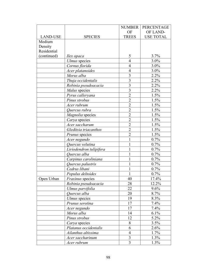
A full recording of species by land-use classification can be found in
Appendix 2. An annotated version of this table has been included in Table 4 for
convenience that lists the 5 most common species of the residential, Forested, Open
Urban, and Transportation plots.
The 37 Medium Density Residential plots with trees included trees originating
from nurseries as well generally undesirable species to use in the landscape. Some of
the most frequently encountered trees within this land-use were popular evergreen
landscape trees, such as Picea abies with 11.9% and Tsuga canadensis with 5.9% of
the trees within these Medium Density Residential plots. Deciduous trees popular in
the landscape were Acer palmatum (5.2%), Cornus florida (3.0%), and ornamental
Prunus species, found in respectable numbers with 1.5%. Also found were most
36
Table 4. A listing of the 5 most prevalent tree species found within 5 of the
most populated land-use classes in the 1999 Baltimore UFORE survey. A
complete listing of species found within land-uses can be found in Appendix
2.
LAND-USE SPECIES NUMBER OF TREES
PERCENTAGE OF LAND-USE
TOTAL High Density Residential Ailanthus altissima 14 20.3% Acer saccharinum 8 11.6% Morus alba 7 10.1% Acer rubrum 6 8.7% Quercus prinus 4 5.8% Medium Density Residential Picea abies 16
in a Shannon’s diversity index of 0.95. Simpson’s Diversity Index, interpreted as a
probability of encountering a species again in an area, is included in the data set as it
is more intuitive. The index and the relative rankings are not discussed as results
were similar to the Shannon’s Diversity Index.
Detrended correspondence analysis of tree species across land-uses
A DCA ordination (Figure 4) was used to examine possible environmental
gradients influencing tree species distribution based on land-use classification. The
total variance accounted for in the species data, or the inertia, was 9.196. There are
no significance tests associated with DCA to report.
In a DCA scatterplot, Axis 1 explains the principal sources of compositional
variation while higher order axes explain progressively less of the variation. As a
modified reciprocal averaging ordination, environmental gradients affecting the
species compositional response, or other factors, may be indicated by positioning
along Axis 1. In essence, species that are found in similar habitats should be found
within close proximity along Axis 1, while plots that are similar in tree composition
should be grouped in a similar fashion. If Hypothesis 1 is correct and plots of the
same land-use contained similar species, then there should be a clear pattern of plots
being arranged by land-use, clustered horizontally along Axis 1.
In this analysis, however, the distribution of plot scores across the first axis
yielded no obvious visual pattern of plots clustering based on land-use classification.
The large amount of overlap of land-uses along Axis 1 (Figure 4A) indicated that
either contrasting environmental or management conditions that would be assumed to
42
ACNE
ACPA
ACPL
ACRU
ACSA1ACSA2
AIAL
CA1
CACA
COFLFAGR
FR
LITU MOALNYSY
PIABPR
PRSE1
PYCA
QUAL
QUPH
QURU
QUVE
ROPS
SAAL
THOC
TSCA
ULS
0
100
200
300
400
500
600
0 100 200 300 400 500 600 700
Axis
2
Axis 1
FIG. 4a and 4b. A Detrended Correspondence Analysis ordination graph of the vegetation data from the UFORE survey of Baltimore, MD in 1999. The first two axes DCA ordination axes from PCORD Version 4.41. Axes are scaled in 100 3 SD beta diversity units (Hill and Gauch, 1980). (A) Sample scores for 100 plots within 6 land-use types. (B) Species scores for 28 tree species (see App. 1).
0
100
200
300
400
500
600
0 100 200 300 400 500 600 700
Axis 1
Axi
s 2
C om merc ial
F ores ted
H igh dens ityre si denti alM edium dens it yre si denti alO pen urban
T ransport ation
43
characterize the different land-uses does not appear to explain tree species
distribution or that the cityscape is too homogenized across land-uses to produce
discrete compositional groups.
Perhaps the only exception was Medium Density Residential plots, which
appear to cluster slightly at the right hand side of Axis 1 around the score of 500
standard deviation units. This may be due to the presence of a number of unique
exotic species that were planted by homeowners that could not be found elsewhere in
other land-uses as they do not naturalize in the area.
Tree species scores within this ordination (Figure 4B) may, however, present
a slight pattern indicating that there a possibility that land-use classification may
partly explain tree species distribution. There was a general grouping of tree species
towards the left side of Axis 1 that are usually almost exclusively found in forested
areas including Fagus grandifolia, Liriodendron tulipifera, Carpinus caroliniana, and
Nyssa sylvatica. There was also a second clustering of species found generally only
within planted landscapes in the Baltimore region that can be found to the far right
section of axis 1 including Acer palmatum, Thuja occidentalis, and Picea abies. A
third clustering of species generally confined to the edges of forests, disturbed areas,
roadsides, and fenced yards can be found in between the two mentioned previously
groups. These disturbed and edge-site dwelling species consisted of Robinia
pseudoacacia, Morus alba, and Ailanthus altissima. Two outlying species were
Sassafras albidum and Tsuga Canadensis.
44
Figure 5. A map of Baltimore City’s census tracts used in the 2000 US
Census and the corresponding locations of the 200 plots from the 1999
UFORE vegetation survey.
45
The relationship between socioeconomic variables and tree species composition
Canonical correspondence analysis was utilized in order to evaluate the
correlation of social economic factors and non-natural environmental factors with the
distribution of tree species. Data was taken from the 2000 United States
Census based on data for census tracts to represent plot socioeconomic data with the
assumption that census tracts are relatively small, homogenous areas that are
comparable for statistical purposes (Figure 5).
Table 6. Variables used in canonical correspondence analysis
taken in the 2000 United States Census of Baltimore City, MD
The first canonical correspondence analysis was run using socio-economic
variables from the 2000 Census (Table 6). Variables in this analysis related to the
2000 Census Bureau Data Variable
Range Present in Baltimore City
Population Density 1.6 - 41.4 people per acre
Median Household Income
$11,840 - $71,771 per year
Percent Vacant Housing
0 - 30%
Median Age of Structure on Property
27 - 68 years
Percent Impervious Surface on Plot
0 - 100%
46
tree species abundance matrix included: population density, median annual household
income, and percent vacant housing (Table 6). The locations of the plots, represented
by triangles on a CCA scatterpoint graph, indicate the environmental characteristics
of the plot and the positions of the species on the plot, represented by both plus signs
and the species codes, indicate the relationship of the variables and the tree species.
Plot locations spatially reflect similarities in species composition and in
environmental variable values (Jongman, 1987).
In the ordination biplot, variables are represented by vectors shown as arrows
on the plot. The magnitudes of the arrows indicate importance of the environmental
variables in accounting for the variation in species composition within the plots.
Visually, the CCA graph of the census information of the plots (Figure 6) shows short
arrow lengths that encompass only a fraction of the plots in the ordination and do not
appear to be important in explaining tree species distribution. The direction of the
arrow indicates the correlation of the variable with the axes and with other variables,
with smaller angles between vectors and axes indicating closer association. By
direction, Population Density and Median Household Income were not correlated.
Percent Vacant Housing did not appear on the biplot as it was not important in the
first two axes.
The total variance or inertia, or the total amount of variability in the
community matrix that could potentially be explained, was 12.5359 with 3 canonical
axes interpreted. Eigenvalues represent the variance in the community matrix
accounted for by each axis as well as the correlation of the species scores and the site
scores with a value near 1 indicating a strong relationship. As expected, the
47
eigenvalue was greatest for the first axis at 0.321, and then decreased for the second
and third axes at 0.252 and 0.160, respectively.
Figure 6. Canonical correspondence analysis biplot of 2000 Baltimore
City Census Data figures for Population Density, Median Household
Income, and Percent Vacant Housing. The symbols are as follows: ∆
represent plots, + represent tree species.
48
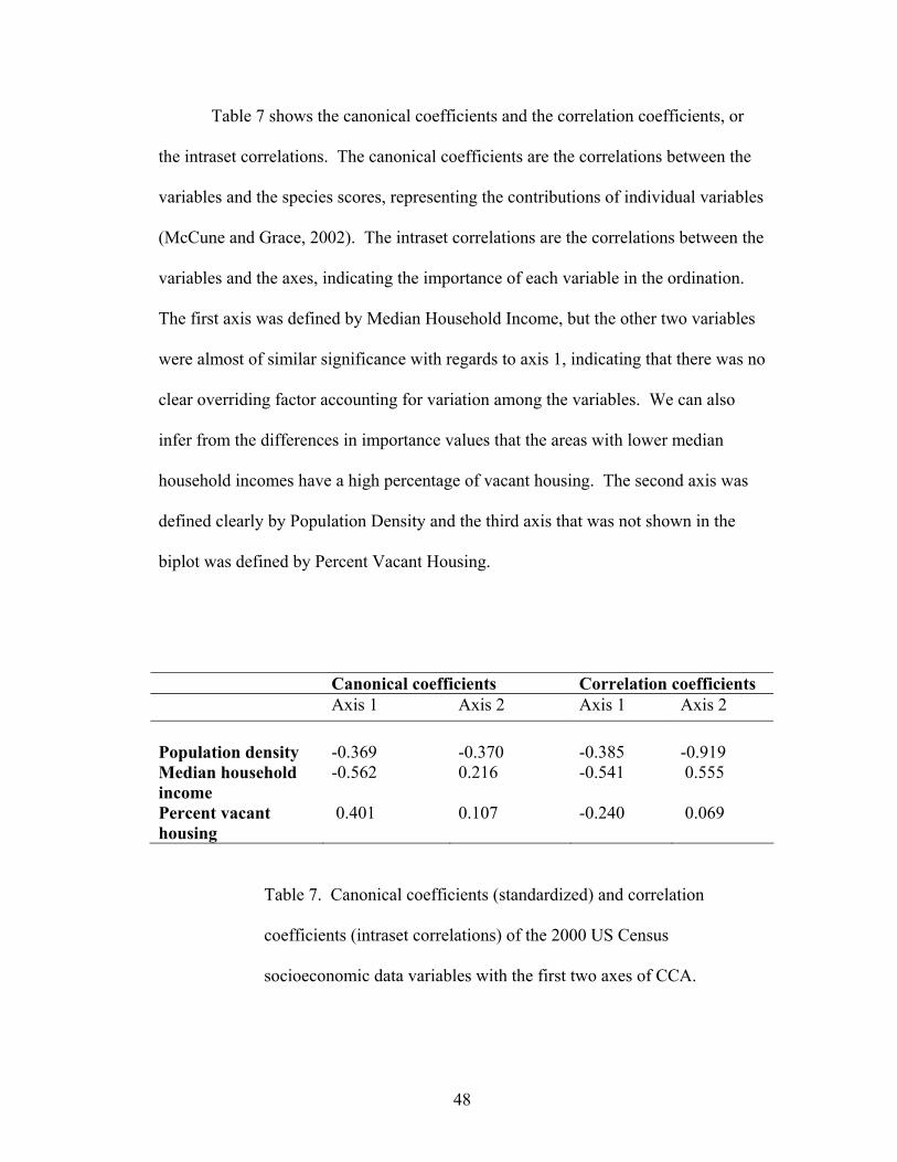
Table 7 shows the canonical coefficients and the correlation coefficients, or
the intraset correlations. The canonical coefficients are the correlations between the
variables and the species scores, representing the contributions of individual variables
(McCune and Grace, 2002). The intraset correlations are the correlations between the
variables and the axes, indicating the importance of each variable in the ordination.
The first axis was defined by Median Household Income, but the other two variables
were almost of similar significance with regards to axis 1, indicating that there was no
clear overriding factor accounting for variation among the variables. We can also
infer from the differences in importance values that the areas with lower median
household incomes have a high percentage of vacant housing. The second axis was
defined clearly by Population Density and the third axis that was not shown in the
biplot was defined by Percent Vacant Housing.
Canonical coefficients Correlation coefficients Axis 1 Axis 2 Axis 1 Axis 2 Population density -0.369 -0.370 -0.385 -0.919 Median household income
-0.562 0.216 -0.541 0.555
Percent vacant housing
0.401 0.107 -0.240 0.069
Table 7. Canonical coefficients (standardized) and correlation
coefficients (intraset correlations) of the 2000 US Census
socioeconomic data variables with the first two axes of CCA.
49
The relationships between environmental factors and species composition can
be tested using Monte Carlo permutation with 999 runs employed at the 5%
significance level (Ter Braak and Smilauer, 2002). The Monte Carlo permutation test
will test the significance of the first axis eigenvalue (ter Braak, 1990). The first
hypothesis will test the null hypothesis that there is no linear relationship between
matrices, or in other words, that the community composition is unrelated to the
environmental variables. The Monte Carlo tests for this analysis had a p-value of
0.1790, indicating that the variance is not explained by these variables. Also, the
Species-Environment Correlation had a non-significant p-value of 0.2770, therefore,
the matrices are not correlated and sites with the same social economic factors do not
have the same species. Correlates are not discussed as there was no relationship
found.
As some of the land-uses may not be sensitive to socioeconomic impacts on
tree species composition and may confound the results of those that are, a secondary
CCA was utilized with data solely from the residential plots. Medium Density and
High Density Residential vegetation data was entered separately as the main matrix
along with the same census information as above. For this analysis, trees that
occurred in more than 3 plots and with more than 4 total individuals, totaling 21
species within 56 plots, were included.
The joint biplot again shows arrows that are short of encompassing all of the
sites (Figure 7). Unlike the previous analysis, the variable percent vacant housing
appears on the biplot. The total variance in the species data was 10.7017 with 3
canonical axes. The eigenvalue of the first axis was 0.472 and accounted for 4.4% of
50
Figure 7. Reduced canonical correspondence analysis biplot using
High Density and Medium Density Residential plots with the 2000
Baltimore City Census Data figures for Population Density, Median
Household Income, and Percent Vacant Housing. The symbols are as
follows: ∆ represent plots, + represent tree species.
ACPA
ACPL
ACRU
ACSA1AIAL
COFL
FRSP
ILOP
JUVI
MA2
MAGSP
MOAL
PIABPIST
PRSE1
PRSPPYCA
QURU
THOC
TSCA
ULSPPopulation Density
Median Household IncomePercent Vacant Housing
00
20 40 60 80
40
80
Axis 1
Axi
s 2
51
the variance explained by this analysis. The first axis was explained by Median
Household Income, while the second axis, unlike the previous analysis with all land-
uses, was explained by Percent Vacant Housing.
The first hypothesis test of the Monte Carlo results had a significance of
0.0420 and the variance summarized by the first axis could be meaningfully
interpreted. The second test showed that there was not a significant relationship
between the species compositions and the socioeconomic data with a p value of
0.1910. Therefore, socioeconomic factors alone could not account for the variance in
data in the residential plots.
The relationship between anthropogenic environmental variables and tree species composition
A canonical correspondence analysis was performed with the species matrix
using the non-natural environmental factors median age of structure and percent
impervious surface cover. Median age of structure on property, taken from data from
the 2000 US Census, is used here as an indication of the last time that a construction
disturbance occurred on the plot. For example, newer residential developments on
the edges of the city could be expected to have had recent major land-clearing
projects, whereas residential developments constructed earlier in the century or prior
may have less disturbed landscape areas. Percent impervious surface of the
individual plots was taken directly from the survey data and indicates the amount of
concrete, paved roadways and driveways, and building. The average percent of
impervious surface by land-use is shown in Table 8.
52
Table 8. The average percent surface impervious cover
calculated from groundpoints for each land-use of the 200 plots
counted in the Baltimore, MD UFORE vegetation survey.
The biplot indicated that there was no correlation between the two variables as
their directions were nearly perpendicular and the correlation among the variables
was very low (Figure 8); the weighted correlation being -0.027 (data not shown). The
environmental variables are related to the first axis fairly well (Table 9), and are
poorly related to the second axis. The first axis is defined by percent impervious
surface cover (Table 10) and the second axis is defined by median structure age on
Land-use Avg % imp.
surface Commercial 76% Industrial 64% High Density Residential 61% Institutional 50% Transportation 44% Medium Density Res. 44% Open Urban 22% Forested 10% Bare Ground 0%
53
Figure 8. Canonical correspondence analysis of 2000 Baltimore City
Census Data figures for Median Age of Structure and Percent
Impervious Surface of the pot. The symbols are as follows: ∆
represent plots, + represent tree species.
54
Table 9. Eigenvalues and Pearson Species-Environment correlation
coefficients for the first two axes of the CCA analysis of tree species
abundances with anthropogenic environmental coefficients.
property. The total variance, or inertia, of the species data was 12.536, and the
percent variance explained for the first axis was 3.2%.
A Monte Carlo Test did indicate a significant result with the Eigenvalue
having a p-value of 0.0100 and the Species-Environment Correlation with a p-value
of 0.0300. The hypothesis of no relationship between the species data and the
environmental data is rejected as the eigenvalue for the first axis, representing the
variance in the community matrix accounted for by the first axis, is much higher than
expected by chance. Percent Impervious Surface Cover was apparently more of a
factor in this significant result as the canonical coefficients for this variable was
-0.983 with Axis 1 and Median Age of Structure was only 0.209 for Axis 1 (Table
10). This indicates that some of the variance can be explained by the amount of
Axis 1 Axis 2
Eigenvalue 0.401 0.128
Variance in species data % explained
3.2 1.0
Pearson Correlation, species-environment
0.33 0.506
55
Table 10. Canonical coefficients and intraset correlations of anthropogenic
environmental variables with the first two axes of CCA.
impervious surface cover on the plots, essentially describing the degree of
urbanization, and that plots with similar amounts of impervious surface cover had
similar species.
This can be seen with the species denoted on the biplot (Figure 8). Species at
the opposite end of the arrowhead of percent impervious cover are those that would
likely be found in plots with little impervious surface. These species include a variety
of species generally confined to forested environments, such as Fagus grandifolia,
Nyssa sylvatica, and Carya species. While species at the opposite end, such as
Ailanthus altissima, Pyrus calleryana, and Acer saccharinum, are species typically
found near areas of high percentages of impervious groundcover.
MA2 Malus species crabapple Exotic MA1 Magnolia species magnolia Exotic MOAL Morus alba white mulberry Invasive
95
* The category of Native/Exotic/Invasive was determined through personal knowledge and with the aid of Burns and Honkala (1990).
CODE SCIENTIFIC NAME COMMON NAME
Native/ Invasive/ or Exotic to Baltimore
NYSY Nyssa sylvatica blackgum Native
OSVI Ostrya virginiana American hophornbeam Perhaps native to western portions
PIAB Picea abies Norway spruce Exotic PIST Pinus strobus eastern white pine Native
PLOC Platanus occidentalis American sycamore Native
PODE Populus deltoides eastern poplar Uncertain PR Prunus species flowering cherry Exotic PRSE1 Prunus serotina black cherry Native
PYCA Pyrus calleryana Callery pear Invasive QUAC Quercus acutissima sawtooth oak Invasive QUAL Quercus alba white oak Native QUCO Quercus coccinea scarlet oak Native QUFA Quercus falcata southern red oak Native QUPA Quercus palustris pin oak Native QUPH Quercus phellos willow oak Native QUPR Quercus prinus chestnut oak Native QURU Quercus rubra red oak Native QUVE Quercus velutina black oak Native ROPS Robinia pseudoacacia black locust Exotic SAAL Sassafras albidum sassafras Native THOC Thuja occidentalis American arborvitae Exotic TIAM Tilia americana basswood Exotic
TICO Tilia cordata littleleaf linden Exotic
TSCA Tsuga canadensis eastern hemlock Exotic ULPA Ulmus parvifolia chinese elm Invasive ULSP Ulmus species elm Native
Abrams, M.D. 1992. Fire and the development of oak forests. BioScience 42:346–353. Alban, D.H. 1982. Effects of nutrient accumulation by aspen, spruce, and pine on soil properties. Soil Science Society of America Journal 46:853-861. Barnes, B.V. 1991. Deciduous Forests of North America. In E. Röhrig and B. Ulrich (eds.), Ecosystems of the World, Temperate Deciduous Forests. Volume 7. Elsevier, New York. Alig, R.J., Kline, J.D., and Lichtenstein, M. 2004. Urbanization on the US landscape: looking ahead in the 21st century. Landscape and Urban Planning 69(2-3):219-234. Augusto, L., Ranger, J., Binkley, D., and Rothe, A. 2002. Impact of several common tree species of European temperate forests on soil fertility. Annals of Forest Science 59(3):233-253. Beckett, K.P., Freer-Smith, P.H., and Taylor, G. 1997. Urban woodlands: their role in reducing the effects of particulate pollution. Environmental Pollution 99(3):347-360. Binkley D., Giardina C. 1998. Why do tree species affect soils? The warp and woof of tree-soil interactions. Biogeochemistry 42:89–106. Boring, L.R., Monk, C.D., and Swank, W.T. 1981. Early regeneration of a clear-cut Southern Appalachian forest. Ecology 62: 1244-1253. Bory, G. and Clair-Maczulajtys, D. 1980. Production, dissemination and polymorphism of seeds in Ailanthus altissima. Revue Generale de Botanique 88:297-311. Borin, M., Vianello, M., Morari, F., and Zanin, G. 2004. Effectiveness of buffer strips in removing pollutants in runoff from a cultivated field in North-East Italy. Agriculture, Ecosystems and Environment 105(1-2):101-114. Brothers, T.S., and Spingarn, A. 1992. Forest fragmentation and alien plant invasion of Central Indiana old-growth forests. Conservation Biology 6:91-100. Brush, G.S., Lenk, C., Smith, J. 1980. The Natural Forests of Maryland: An Explanation of the Vegetation Map of Maryland. Ecological Monographs 50(1): 77-92.
101
Burns, R.M. and Honkala,B.H., tech coords. 1990. Silvics of North America. Agriculture Handbook 654. U.S. Department of Agriculture, Forest Service, Washington, DC. Vol 2, 877 p. Burton, M.L. and Samuelson, L.J. 2008. Influence of urbanization on riparian forest diversity and structure in the Georgia Piedmont, US. Plant Ecology 195(1):99-115. Busing, R.T. 1995. Disturbance and the Population Dynamics of Liriodendron Tulipifera: Simulations with a Spatial Model of Forest Succession. Journal of Ecology 83(1): 45-53. Cadenasso, M.L., Pickett, S.T.A., McDonnell, M.J., and Pouyat, R.V. 2007. Forest vegetation along an urban-rural gradient in the New York City metropolitan area: patterns and relationships to ecosystem processes. Transactions of the Linnean Society of New York 10: 79-99. Chapelle, S., and Ridgway, W. 1986. Maryland: A History of Its People. JHU Press. 352 pages. Chesson, P.L. 2000. General theory of competitive coexistence in spatially varying environments. Theoretical Population Biology 58(3):211-237. Collins, J.P., Kinzig, A., Grimm, N.B., Fagan, W.F., Hope, D., Wu, J., and Borer, E.T. 2000. A new urban ecology. American Scientist 88(5):416-425. Cully, T.M. and Hardiman, N.A. 2007. The beginning of a new invasive plant: A history of the ornamental callery pear in the United States. Bioscience 57(11): 956-964. Davis, M.B., Calcote, R.R., Sugita, S., and Takahara, H. 1998. Patchy invasion and the origin of a hemlock-hardwoods forest mosaic. Ecology 79:2641–2659. Detwyler, T.R. and Marcus, M.G. (eds). 1972. Vegetation of the City: Urbanization and the environment. Duxbury Press, Belmont. Dirr, M.A. 1998. Manual of Woody Landscape Plants: Their Identification, Ornamental Characteristics, Culture, Propagation, and Uses (5th edition). Champaign, IL, Stipes Publishing, L.L.C. Ehrenfeld, J.G., Ravit, B., and Elgersma, K. 2005. Feedback in the plant-soil system. Annual Review of Environment and Resources 30:75-115. Elliott, K.J., Boring, L.R., Swank, W.T., and Haines, B.R. 1997. Successional changes in plant species diversity and composition after clearcutting a Southern Appalachian watershed. Forest Ecology and Management 92: 67-85.
102
Ejrnaes, R. 2000. Can we trust gradients extracted by Detrended Correspondence Analysis? Journal of Vegetation Science 11:565-572. ESRI. 2006. ArcGIS Version 9.2. Redlands, California, Environmental Systems Research Institute.
Eyre, F. H., ed. 1980. Forest cover types of the United States and Canada. Society of American Foresters, Washington, DC. 148 p.
Finzi, A.C., Canham, C.D., Breemen, N.V. 1998. Canopy tree-soil interactions within temperate forests: species effects on pH and cations. Ecological Applications 8(2):447-454. Freedman, B., Love, S., and O’Neil, B. 1996. Tree species composition, structure, and carbon storage in stands of urban forest of varying character in Halifax, Nova Scotia. Canadian Field Naturalist 110(4):675-682. Freer-Smith, P.H., Holloway, S., and Goodman, A. 1997. The uptake of particulates by an urban woodland: site description and particulate composition. Environmental Pollution 95(1):27-35. Frelich, L.E. 2002. Forest Dynamics and Disturbance Regimes: Studies from Temperate Evergreen—Deciduous Forests. Cambridge University Press, Cambridge, UK.
Godefroid, S., and Koedam, N. 2003. Distribution pattern of the flora in a peri-urban forest: an effect of the city–forest ecotone. Landscape and Urban Planning 65: 169-185.
Grimes, J.P. 1979. Plant Strategies and Vegetation Processes. John Wiley & Sons, Chichester, UK. Groffman, P.M, Bain, D.J., Bland, L.E., Belt, K.T., Brush, G.S., Grove, J.M., Pouyat, R.V., Yesilonis, I.C., and Zipperer, W.C. 2003. Down by the riverside: urban riparian ecology. Frontiers in Ecology and the Environment 1(6):315-321. Groffman, P. M., Pouyat, R.P., McDonnell, M.J., Pickett, S. T. A., and Zipperer, W. C. 1995. Carbon pools and trace gas fluxes in urban forest soils. Pages 147–158 in R. Lat, J. Kimble, E. Levine, and B. A. Steward, editors. Advances in soil science: Soil management and greenhouse effect. CRC Press, Boca Raton, Florida. Grove, J.M. 1996. The relationship between patterns and processes of social stratification and the vegetation of an urban-rural watershed. School of Forestry and Environmental Studies. New Haven: Yale University.
103
Grove, J.M., Troy, A.R., O’Neil-Dunne, J.P.M, Burch, Jr., W.R., Cadenasso, M.L., and Pickett, S.T.A. 2006. Characterization of households and its implications for the vegetation of urban ecosystems. Ecosystems 9(4):578-597. Guirado, M., Pino, J., Roda, F. and Basnou, C. (2008). Quercus and Pinus cover are determined by landscape structure and dynamics in peri-urban Mediterranean forest patches. Plant Ecology 194(1):109-119. Harris, L.D., and Sanderson, J. 2000. The remembered landscape. In Landscape Ecology: A Top Down Approach. Sanderson, J., and Harris, L.D. (eds). Boca Raton, Fl, CRC press, 91-112. Hill, M.O. 1979. DECORANA: A FORTRAN program for detrended correspondence analysis and reciprocal averaging. Ecology and Systematics. Cornell University, Ithaca, NY. Hill, M.O. and Gauch, Jr., H.G. 1980. Detrended correspondence analysis: an improved ordination technique. Vegetatio 42:47-58. Hope, D., Gries, C., Zhu, W., Fagan, W.F., Redman, C.L., Grimm, N.B., Nelson, A.L., Martin, C., and Kinzig, A. 2003. Socioeconomics drive urban plant diversity. Proceedings of the National Academy of Sciences USA 100(15): 8788-92. Hu, S.Y. 1979. Ailanthus. Arnoldia 39(2):29-50. Hutchinson, M. F. 1957. Concluding remarks. Cold Spring Harbour Symposium on Quantitative Biology 22:415–427.
Hutnick, R.J., and Yawney, H.W. 1961. Silvical characteristics of red maple (Acer rubrum). USDA Forest Service, Station Paper 142. Northeastern Forest Experiment Station, Upper Darby, PA. 18 p.
Inderjit and Duke, S. 2003. Ecophysiological Aspects of Allelopathy. Planta 217:529-539.
Jongman, R.H.G., ter Braak, C.J.F. and van Tongeren, O.F.R. 1987. Data analysis in community and landscape ecology. Pudoc, Wageningen. Karl, T.R., Diaz, H., and Kukla, G. 1988. Urbanization: Its detection and effect in the United States Climate Record. Journal of Climate 1(11): 1099-1123. Kent, M. and Coker, P. 1992. Vegetation Description and Analysis, A Practical Approach. John Wiley and Sons, New York, pp 167-169. Kricher, J. 1998. A Field Guide to Eastern Forests. Houghton Mifflin Company, New York, 488 pages.
104
Kuers, K.. 2005. “Watershed Procedures Manual: Procedures.” Ranking Species Contribution to Forest Community Composition: Calculation of Importance Values. 25 July 2005. Sewanee: The University of the South. 13 August 2008 <http://www.sewanee.edu/Forestry_Geology/watershed_web/Emanuel/ImportanceValues/ImpVal_SET.html>. Lavorel, S. and Garnier, E. 2002. Predicting changes in community composition and ecosystem functioning from plant traits: revisiting the Holy Grail. Functional Ecology 16(5):545-556. Little, Elbert L., Jr. 1971. Atlas of United States trees, vol. 1. Conifers and important hardwoods. U.S. Department of Agriculture, Miscellaneous Publication 1146. Washington, DC.
Little, Elbert L., Jr. 1979. Checklist of United States trees (native and naturalized). U.S. Department of Agriculture, Agriculture Handbook 541. Washington, DC. 375 p.
Lowenstein, N.J., and Lowenstein, E.F. 2005. Non-native plants in the understory of riparian forests across a land-use gradient in the Southeast. Urban Ecosystems. 8(1):7-21. Lou, Z.K., Sun O.J.,, Ge Q.S., Xu, W.T., and Zheng, J.Y. (2007). Phenological responses of plants to climate change in an urban environment. Ecological Research 22(3):507-514. Mack, R.N., Simberloff, D., Lonsdale, W.M., Clout, M., and Bazzaz, F.A. 2000. Biotic invasions: causes, epidemiology, global consequences, and control. Ecological Applications 10:689-710.
Mandryk, A.M. and R.W. W. 2006. Exotic vascular plant invasiveness and forest invisibility in urban boreal forest types. Biological Invasions 8(8): 1651-1662.
Martin, C.A., Warren, P.S., and Kinzig, A. 2004. Neighborhood socioeconomic status is a useful predictor of perennial landscape vegetation in small parks surrounding residential neighborhoods in Phoenix, Arizona. Landscape Urban Planning 69:355-368.
McClenahen, J.R. 1978. Community changes in a deciduous forest exposed to air pollution. Canadian Journal of Forest Research 8(4):38-43. McCune, B. and J.B. Grace. 2002. Analysis of Ecological Communities. Gleneden Beach, Oregon, MjM Software Design. McCune, B. and Mefford, M.J. 1999. Multivariate Analysis of Ecological Data, MjM Software, Gleneden Beach, Oregon, U.S.A.
105
McDonald, R.I., and Urban, D.L. 2006. Edge effects on species composition and exotic species abundances in the North Carolina piedmont. Biological Invasions 8(5): 1049-1060. McDonnell, M.J., Pickett, S.T.A., Groffman, P., and Bohlen, P. 1997. Ecosystem processes along an urban-to-rural gradient. Urban ecosystems 1(1):21-36. McDonnell, M.J. and Pickett, S.T.A., Likens, G.E., and Cronon, W.J. 1993. Humans as components of ecosystems: the ecology of subtle human effects and populated areas. New York, Springer-Verlag. McDonnel, M.J. and Pickett, S.T.A. 1990. Ecosystem structure and function along urban-rural gradients – an unexploited opportunity for ecology. Ecology 71(4): 1232-1237. McKinney, M.L. 2006. Urbanization as a major cause of biotic homogenization. Biological Conservation 127(3):247-260. McPherson, E.G., Nowak, D.J., and Rowntree, R.A., eds., pp 3-18. USDA For. Serv. Gen. Tech. Rep. NE-186. Medley, K.E., MJ McDonnell, and Pickett, S.T.A. 1995. Forest-landscape structure along an urban-to-rural gradient. The Professional Geographer 47(2):159-168. Meiners, S.J., S.T.A. Pickett, and Cadenasso, M.L. 2001. Effects of plant invasions on the species richness of abandoned agricultural land. Ecograhy 24(6):633-644. Mergen, F. 1959. A toxic principle in the leaves of Ailanthus. Botanical Gazette 121:32-36. Minchin, P. 1987. An evaluation of the relative robustness of techniques for ecological ordination. Vegetatio 69:89-107. Mofatt, S.F., McLachlan, S.M., and Kenkel, N.C. 2004. Impacts of land use on riparian forest along an urban-rural gradient in Southern Manitoba. Plant Ecology 174(1):119-135. Mohan, J.E., Clark, J.S., and Schlesinger,W.H. 2007. Long-term CO2 enrichment of a forest ecosystem: Implications for forest regeneration and succession. Ecological Applications 17(4):1198-1212. NOAA. 2004. Climatography of the United States #60, Climates of the States. N.C.D.C. United States Department of Commerce.
106
Nowak, D.J. 1993 Atmospheric carbon reduction by urban trees. Journal of Environmental Management 37(3):207-217. Nowak, D.J. 1994a. Urban Forest Structure: the state of Chicago’s urban forest. In Chicago’s urban forest ecosystem: results of the Chicago Urban Forest Climate Project, (E. G. McPherson, D. J. Nowak and R. A. Rowntree, eds.), pp. 3–18. USDA Forest Service, Northeastern Forest Experiment Station, Radnor. Gen. Tech. Rep. NE-186. Nowak, D.J. 1994b. Air pollution removal by Chicago’s urban forest. In Chicago’s urban forest ecosystem: results of the Chicago Urban Forest Climate Project, E.G. McPherson, D.J. Nowak, and R.A.Rowntree, eds., pp 63-81. USDA For. Serv. Gen. Tech. Rep. NE-186. Nowak, D.J. 1994c. Atmospheric carbon dioxide reduction by Chicago’s urban forest. In Chicago’s urban forest ecosystem: results of the Chicago Urban Forest Climate Nowak, D.J. (1994d). Understanding the structure of urban forests. Journal of Forestry 92(10):42-46. Nowak, D.J., Noble, M.H., Sisinni, S.M., and Dwyer, J.F. 2001. Assessing the U.S. urban forest resource. Journal of Forestry 99(3):37-42. Nowak, D.J. and D.E. Crane. 2000. The Urban Forest Effects Model: Quantifying urban forest structure and functions. In: Proceedings Integrated Tools for Natural Resources Inventories in the 21st Century. IUFRO Conference, 16-20 August 1998, Boise, ID. General Technical Report NC-212, U.S. Department of Agriculture, Forest Service, North Central Research Station, St. Paul, MN. Nowak, D.J., D.E. Crane, et al. 2002. Understanding and Quantifying Urban Forest Structure, Functions, and Value. 5th Canadian Urban Forest Conference, Region of York, Ontario. Nowak, D.J., Stevens, J.C., et al. 2005. The Urban Forest Effects (UFORE) Model: Field Data Collection Manual. N.R.S. USDA Forest Service. Found at http://www.fs.fed.us/ne/syracuse/Tools/downloads/UFORE_Manual.pdf. Nowak, D.J., Crane, D.E., Stevens, J.C., Hoehn, R.E., Walton, J.T., Bond, J. 2008. A ground-based method of assessing urban forest structure and ecosystem services. Arboriculture and Urban Forestry 34(6):347-358. Oke, T.R. 1989. The micrometeorology of the urban forest. Philosophical Transactions of the Royal Society of London. Series B, Biological Sciences (1934-1990) 324(1223): 335-349.
107
Oke, T.R. 1995. The heat island of the urban boundary layer: characteristics, causes and effects. In Wind Climate in Cities, ed JE Cermak. 81-107. Netherlands: Kluwer Academy. Okland, R.H. 1990. Vegetation ecology: theory, methods and applications with reference to Fennoscandia. Sommerfeltia Suppl. 1:1-230. Palmer, Michael.1993. Putting things in even better order: The advantages of canonical correspondence analysis. Ecology 74 (8): 2215-2230. Pickett, S.T.A., Kolasa, J., Armesto, J.J., Collins, S.L. 1989. The ecological concept of disturbance and its expression at different hierarchical levels. Oikos 54(2):129-156. Pickett, S.T.A., Burch, W.R., Dalton, S.E., Foresman, T.W., Grove, J.M., and Rowntree, R.A. 1997. A conceptual framework for the study of human ecosystems. Urban Ecosystems 1:185-199. Poland, T.M., and McCullough, D.G. 2006. Emerald ash borer: Invasion of the urban forest and the threat to North America’s ash resource. Journal of Forestry 104(3):118-124. Porter, E.E., B.R. Forschner, and Blair, R.B. 2001. Woody vegetation and canopy fragmentation along a forest-urban gradient. Urban Ecosystems 5(2):131-151. Pouyat, R.V., McDonnel, M.J., Pickett, S.T.A and Groffman, P.M. 1995. Carbon and nitrogen dynamics in oak stands along and urban to rural gradient. In Carbon Forms and Functions in Forest Soils. Pp 569-587. J.M. Kelly and W.W. McFee. Madison, WI: Soil Sci. Soc. Am. Pouyat, R.V., Yesilonis, I.D., Russell-Anelli, J. 2007. Soil chemical and physical properties that differentiate urban land-use and cover types. Soil Science Society of America Journal 71(3): 1010-1019. Reich, P.B., Oleksyn, J., Modrzynski, J., Mrozinski, P., Hobbie, S.E., Eissenstat, D.M., Chorover, J., Chadwick, O.A., Hale, C.M., and Tjoelker, M.G. 2005. Linking litter calcium, earthworms and soil properties: a common garden test with 14 tree species. Ecology Letters 8(8):811-818. Rizzo, D.M., Garbelotto, M., Davidson, J.M., Slaughter, G.W., and Koike, S.T. 2002. Phytophthora ramorum as the cause of extensive mortality of Quercus spp. And Lithocarpus densiflorus in California. Plant Disease 86 (3): 205-214. Robinson, G.R. and S.N. Handel. 1993. Forest restoration on a closed landfill: Rapid addition of new species by bird dispersal. Conservation Biology 7(2):271-278.
108
Rogers, J.E. 1935. The Tree Book. Doubleday, Doran and Co., Inc. New York. 563 pages. Sax, D.F., and Gaines, S.D. 2003. Species diversity: from global decreases to local increases. Trends in Ecology & Evolution 18(11):561-566. Shea, K. and Chesson, P. 2002. Community ecology theory as a framework for biological invasions. Trends in Ecology and Evolution 17(4):170-176. Shigo, A.L. 1958. Fungi isolated from oak-wilt trees and their effects on Ceratocystis-Fagacearum. Mycologia 50(5):757-769. Simmons, M.E., Wu, X.B., and Whisenant, S.G. 2007. Bottomland hardwood forest species responses to flooding regimes along an urbanized gradient. Ecological Engineering 29:223-231.
Smith, D., 1992. Oak regeneration: The scope of the problem. In: Loftis, D.L.C.E.M. (Ed.), Oak Regeneration: Serious Problems, Practical Recommendations, 8–10 September, Knoxville, TN, USDA Forest Service, General Technical Report SE-84. pp. 40–53. Statler, R. 1984. The plant communities on four landfill sites, New York City, New York. Proceedings of the Northeastern Weed Science Society 38:64-71. Steinberg, D.A., Pouyat, R.V., and Groffman, P.M. 1997. Earthworm abundance and nitrogen mineralization rates along an urban-rural land use gradient. Soil Biology and Biochemistry 29(3-4):427-430. Stokstad, E. 2004. Nurseries may have shipped sudden oak death pathogen nationwide. Science 303:1959. Swearingen, J., K. Reshetiloff, B. Slattery,and S. Zwicker. 2002. Plant Invaders of Mid-Atlantic Areas. National Park Service and U.S. Fish and Wildlife Service, 82 pp. Tabacchi, E., Lambs, L., Guilly, H., Planty-Tabacchi, A.M., Muller, E., and Decamps, H. 2000. Impacts of riparian vegetation on hydrological processes. Hydrological Processes 14(16-17):2959-2976. Ter Braak, C.J.F. 1986. Canonical correspondence analysis: A new eigenvector technique for multivariate direct gradient analysis.Ecology 67:1167-1179. Ter Braak, C.J.F. 1988. CANOCO: A FORTRAN program for canonical community ordination by partial detrended canonical correlation analysis, principal components analysis and redundancy analysis. Microcomputer Power, USA.
109
TWC. 2007. Monthly averages for Baltimore, MD, The Weather Channel Interactive, Inc. at www.weather.com. UFORE Random Plot Selection Tool, U.S. Forest Service, Northeastern Research Station found at http://www.fs.fed.us/ne/syracuse/Tools/tools.htm. United Nations. 2005. World population prospects: the 2004 revision. Department of Economic and Social Affairs, Population Division. New York. USCB. 1980. United States Bureau of Census: Census user’s guide. United States Department of Commerce. United States Government Printing Office, Washington, D.C. USA. USCB. 2000. 2000 Census of Population and Housing, Summary File 1 at http://factfinder.census.gov. United States Census Bureau. USCB, 2005. (www.census.gov; March 19, 2005) USCB. 2007. Topologically Integrated Geographic Encoding and Referencing System at http://www.census.gov/geo/www/tiger/. G.D. United States Census Bureau. USCB. 2008. U.S. Census Bureau: State and County QuickFacts. 15 August 2008. U.S. Census Bureau. 28 July 2008. < http://quickfacts.census.gov/qfd/ tates /24/2404000.html> USDA. 2004a. USDA Forest Service: Effects of urban forests and their management on human health and environmental quality. January 20, 2004. City Urban Forest Data: Boston, Massachusetts. January 6, 2009. <http://www.fs.fed.us/ne/syracuse/Data/State/data_MA_bos_ufore.htm> USDA. 2004b. USDA Forest Service: Effects of urban forests and their management on human health and environmental quality. January 16, 2004. City Urban Forest Data: New York City, New York. January 6, 2009. <http://www.fs.fed.us/ne/syracuse/Data/State/data_NY_nyc_ufore.htm> USDA. 2004c. USDA Forest Service: Effects of urban forests and their management on human health and environmental quality. February 12, 2004. City Urban Forest Data: Baltimore, MD. January 6, 2009. http://www.fs.fed.us/ne/syracuse/Data/State/data_MD_bal_ufore.htm USGS, 2008. USGS Geographic Names Information System (GNIS). 17 November 2008. US Department of the Interior/US Geological Survey. 17 November 2008. <http://geonames.usgs.gov/pls/gnispublic>
110
Vallet, J., Daniel, H., Beaujouan, V., and Roze, F. 2008. Plant species response to urbanization: comparison of isolated woodland patches in two cities of North-Western France. Landscape Ecology 23: 1205-1217. Van Breeman, N., Finzi, A.C., Canham, C.D. 1997. Canopy tree-soil interactions within temperate forests: effects of soil elemental composition and texture on species distributions. Canadian Journal of Forest Research 27:1110-1116. Verheyen, K., Vanhellemont, M., Stock, T., and Hermy, M. 2007. Predicting patterns of invasion by black cherry (Prunus serotina Ehrh.) in Flanders (Belgium) and its impact on the forest understory community. Diversity and Distributions 13:487-497. Vitousek, P.M. 1994. Beyond global warming: ecology and global change. Ecology 75: 1861-1876. Vogt K.A., Grove J.M., Asbjornsen H., Maxwell K., Vogt D.J., Sigurdardottir R., and Dove, M. 2002. Linking ecological and social scales for natural resource management. In Liu J., Taylor W.W. (eds). Integrating landscape ecology into natural resource management. Cambridge (UK): Cambridge University Press. Whitney, G.G. and Adams, S.D. 1980. Man as a maker of new plant communities. Journal of Applied Ecology 17(2):431-448. York, T.E., Dabydeen, S., Smallidge, P. 2000. Understory vegetation-environment relationships in clearcut and mature secondary forests in Western Maryland. Northeastern naturalist 7(3):205-220.