ABSTRACT Title: ANALYSIS OF HOLD TIMES FOR GASEOUS FIRE

ABSTRACT

Title: ANALYSIS OF HOLD TIMES FOR GASEOUS FIRE SUPPRESSION

AGENTS IN TOTAL FLOODING APPLICATIONS

Sean O’Rourke, Master of Science, 2005

Advisor: Frederick W. Mowrer, Associate Professor,

Department of Fire Protection Engineering

Many of the clean agents currently used in total flooding fire suppression applications

have vapor densities greater than ambient air. The denser agent-air mixture creates

hydrostatic pressure differences causing flow of the mixture out of the enclosure as well

as flow of ambient air in through leakage paths inherent in building construction. Hold

time refers to the amount of time it takes for the concentration of the agent-air mixture to

drop below a specified concentration at a designated height within the protected

enclosure. In this study an experimental test enclosure was used to evaluate an analytical

model of agent-air mixture leakage and to investigate the effects of different leakage

areas on agent hold times. The analytical model, known as the descending interface

model, demonstrated favorable agreement with experimental measurements for heights

greater than one-half the height of the enclosure for the agent used in this investigation.

ANALYSIS OF HOLD TIMES FOR

GASEOUS FIRE SUPPRESSION AGENTS IN TOTAL FLOODING

APPLICATIONS

By

Sean Thomas O’Rourke

Thesis submitted to the Faculty of the Graduate School of the University of Maryland, College Park in partial fulfillment

of the requirements for the degree of Master of Science

2005

Advisory Committee: Professor Frederick W. Mowrer, Chair Professor James Milke Professor Peter Sunderland

© Copyright by

Sean Thomas O’Rourke

2005

ii

Acknowledgments

This project was supported by 3M’s Performance Materials Division. I would like to

thank Paul Rivers of 3M for his support and technical guidance while working on this

project. Additionally I would like to thank Dr. Frederick Mowrer, my advisor, for his

assistance, guidance and time while completing this work.

I would also like to thank the other members of my thesis committee, Dr James Milke,

and Dr Peter Sunderland, for their support of this project. Finally, I would like to thank

the faculty and staff, as well as my fellow graduate students, in Fire Protection

Engineering for their help with this work and my time here at the University of Maryland.

iii

Table of Contents

Acknowledgments .......................................................................................... ii Table of Contents........................................................................................... iii List of Figures ................................................................................................ iv List of Tables .................................................................................................. v Chapter 1: Introduction................................................................................... 1

1.1 Background............................................................................................................... 1 1.2 Description of Total Flooding Application............................................................... 3 1.3 Project Objectives ..................................................................................................... 5

Chapter 2: Theoretical Considerations ........................................................... 6 2.1 Literature Review...................................................................................................... 6 2.2 Hydrostatic Pressure Profile within an Enclosure .................................................... 8 2.3 Leakage Area and Flowrate ...................................................................................... 9 2.4 Flow Models ........................................................................................................... 10

2.4.1 Descending Interface Model ............................................................................ 11 2.4.2 Continuous Mixing Model............................................................................... 13 2.4.3 Wide Interface.................................................................................................. 14

2.5 Other Considerations .............................................................................................. 16 2.6 Agent-Air Density................................................................................................... 16 2.7 Leakage Area .......................................................................................................... 19

Chapter 3: Experimental ............................................................................... 21 Chapter 3: Experimental ............................................................................... 21

3.1 Test Apparatus Description..................................................................................... 21 3.2 Experimental Methodology .................................................................................... 25

Chapter 4 Results and Discussion................................................................. 27 4.1 Agent Discharge...................................................................................................... 27 4.2 Concentration Profiles ............................................................................................ 28 4.3 Enclosure Pressure .................................................................................................. 34 4.4 Dimensionless Comparison .................................................................................... 37

Chapter 5: Summary and Conclusions ......................................................... 41 References..................................................................................................... 61 Appendix A: Raw Data and Supplemental Graphs ...................................... 43 Appendix B: Pressure Transducer Calibration Curves................................. 59

iv

List of Figures

Figure 1 Schematic of Total Flooding Clean Agent Application ....................................... 4 Figure 2 Hydrostatic Pressure Profile Schematic ............................................................... 9 Figure 3 Effect of density ratio on velocity ratio.............................................................. 18 Figure 4 Effect of Area Ratio DiNenno and Forssell Analysis ........................................ 19 Figure 5 Effect of Area Ratio Dimensionless Analysis .................................................... 20 Figure 6 Schematic of Test Apparatus, elevation view .................................................... 22 Figure 7 Schematic of Agent delivery system .................................................................. 23 Figure 8 Photograph of (a) Test Apparatus and (b) Agent Delivery System.................... 23 Figure 9 Agent Discharge Nozzle..................................................................................... 24 Figure 10 Inline Pressure Profiles..................................................................................... 27 Figure 11 Temperatures within the enclosure................................................................... 28 Figure 12 Time-Concentration profile, Ao=Ai=0.00038 m2, Co=4.7%............................ 30 Figure 13 Time-Concentration profile, Ao=Ai=0.000253 m2, Co=4.7%.......................... 31 Figure 14 Time-Concentration profile, Ao=Ai=0.000127 m2, Co=4.7%.......................... 32 Figure 15 Time-Concentration profile, Ao=0.000127 m2 Ai=0.00038 m2, Co=4.8% ...... 33 Figure 16 Time-Concentration profile, Ao=0.00038 m2 Ai=0.000127 m2, Co=4.9% ...... 34 Figure 17 Initial Transient Hydrostatic Pressure Profile Ao=Ai=0.00038 m2, Co=4.7%. 35 Figure 18 Hydrostatic Pressure Differences Ao=Ai=0.00038 m2, Co=4.7%.................... 36 Figure 19 Hydrostatic Pressure Differences Ao=Ai=0.000127 m2, Co=4.7%.................. 37 Figure 20 Dimensionless Descending Interface, Experimental data C=80%(Co)............ 38 Figure 21 Dimensionless Descending Interface Experimental data @ C=50%(Co) ........ 40 Figure A 1:Experiment 072805_Test 2 Pressure Profiles Ao=Ai=0.00038 m2................. 46 Figure A 2: Experiment 072805_Test 2 Concentration Profiles Ao=Ai=0.00038 m2...... 46 Figure A 3: Experiment 080105_Test1 Pressure Profiles Ao=Ai=0.00038 m2................. 47 Figure A 4 Experiment 080105_Test1 Concentration Profiles Ao=Ai=0.00038 m2........ 47 Figure A 5 Experiment 080305_Test1 Pressure Profiles Ao=Ai=0.00038 m2.................. 48 Figure A 6 Experiment 080305_Test1 Concentration Profiles Ao=Ai=0.00038 m2......... 48 Figure A 7 Experiment 080305_Test2 Pressure Profiles Ao=Ai=0.000253 m2................ 49 Figure A 8 Experiment 080305_Test1 Concentration Profiles Ao=Ai=0.000253 m2....... 49 Figure A 9 Experiment 080305_Test6 Pressure Profiles Ao=Ai=0.000235 m2................ 50 Figure A 10 Experiment 080305_Test1 Concentration Profiles Ao=Ai=0.000235 m2..... 50 Figure A 11 Experiment 080305_Test3 Pressure Profiles Ao=Ai=0.000127 m2.............. 51 Figure A 12 Experiment 080305_Test3 Concentration Profiles Ao=Ai=0.000127 m2..... 51 Figure A 13 Experiment 080305_Test5 Pressure Profiles Ao=Ai=0.000127 m2.............. 52 Figure A 14 Experiment 080305_Test5 Concentration Profiles Ao=Ai=0.00038 m2....... 52 Figure A 15 Experiment 080505_Test1 Pressure Profiles Ao=Ai=0.000127 m2.............. 53 Figure A 16 Experiment 080505_Test1 Concentration Profiles Ao=Ai=0.000127 m2..... 53 Figure A 17 Experiment 080505_Test3 Pressure Profiles Ao=Ai=0.000127 m2.............. 54 Figure A 18 Experiment 080505_Test3 Concentration Profiles Ao=Ai=0.000127 m2..... 54 Figure A 19 Experiment 080405_Test2 Pressure Profiles Ao=0.000127 m2 Ai=0.00038

m2 .............................................................................................................................. 55 Figure A 20 Experiment 080405_Test2 Pressure Profiles Ao=0.000127 m2 Ai=0.00038

m2 .............................................................................................................................. 55

v

Figure A 21: Experiment 080305_Test2 Pressure Profiles Ao=0.000127 m2 Ai=0.00038 m2 .............................................................................................................................. 56

Figure A 22 Experiment 080305_Test2 Concentration Profiles Ao=0.000127 m2 Ai=0.00038 m2 .......................................................................................................... 56

Figure A 23 Experiment 080405_Test4 Concentration Profiles Ao=0.00038 m2 Ai=0.000127 m2 ........................................................................................................ 57

Figure A 24 Experiment 080405_Test5 Pressure Profiles Ao=0.00038 m2 Ai=0.000127 m2 .............................................................................................................................. 58

Figure A 25 Experiment 080405_Test5 Concentration Profiles Ao=0.000127 m2 Ai=0.00038 m2 .......................................................................................................... 58

List of Tables

Table 1 Common Halon Alternativesa ................................................................................ 2 Table 2 Clean agent density and velocity ratiosa .............................................................. 17 Table 3 Comparison of Leakage Area Scenarios.............................................................. 26 Table A-1 Experimental Raw Data................................................................................... 43

1

Chapter 1: Introduction

1.1 Background

The most popular halogenated fire suppression agent, Halon 1301, was developed

in the 1960’s and quickly saw widespread use in total flooding applications, including the

protection of electrical and electronic equipment, process control rooms, and flammable

liquid and gas storage and transfer facilities. This widespread application of Halon 1301

quickly came to an end under the Montreal Protocol to protect stratospheric ozone. This

agreement among developed countries phased out the production of Halon 1301 as of

January 1, 1994 (DiNenno, SFPE Handbook).

As noted by DiNenno (SFPE Handbook p 4-173), the phase out of Halon 1301 led

to worldwide research and development efforts in search of suitable replacements and

alternatives. Over the past decade many new “halon alternatives” have been developed to

fill this gap in technology. These new “clean” agents are similar to Halon 1301 in that

they vaporize readily, are electrically nonconductive and leave no residue. These agents

fall into two broad categories: halocarbon compounds and inert gases. Some of the

commercialized halon alternatives are listed in Table 1.

2

Table 1 Common Halon Alternativesa

Agent Tradename

Chemical Name ASHRAE designation

Chemical Formula

FE-25 Pentafluroethane HFC-125 C2HF5 FM-200 Heptafluoropropane HFC-227ea C3F7H NAF-SII Dichlorotrifluorethane (4.75%)

Chlorodifluoromethane (82%) Chlorotetrafluoroethane (9.5%) Isopropenyl-1-methylcyclohexane (3.75%)

HCFC Blend A

CHCl2CF3 CHClF2

CHClFCF3

Novec 1230 Dodecafluor-2-methylpentan-3-1 FK-5-1-12 CF2CF2 C(O)CF(CF3)2 Argonite Nitrogen (50%)

Argon (50%) IG-55 N2

Ar Inergen Nitrogen (52%)

Argon (40%) Carbon Dioxide (8%)

IG-541 N2 Ar

CO2 aAdapted from SFPE Handbook 3rd Ed p 4-173

Halocarbon clean agents as well as inert gas fire suppression agents extinguish

fires by physical and chemical mechanisms that depend on the chemical compound. The

dominant suppression mechanism for these agents is the thermal capacity of the gaseous

agent that acts as an energy sink to decrease the flame temperature below that needed to

sustain combustion. Some of the halogenated compounds extinguish a fire by capturing

hydrogen radicals from the fire to interrupt the chemical chain reaction and thus

extinguish the fire, but this effect is less pronounced for the halon alternatives than for

Halon 1301 (DiNenno, SFPE Handbook).

Since these extinguishing mechanisms occur in the gaseous phase, it is important

that the agent concentration necessary to extinguish a fire is maintained for a sufficient

period of time to ensure extinguishment. It is assumed that the discharge of the agent

initially creates a uniform concentration of agent throughout the enclosure. In real-world

enclosures, after the agent is discharged the agent-air mixture will flow through leaks in

3

enclosure boundaries. Flow through these leaks are mainly attributed to pressure

differences due to gas density differences between the inside and outside of the enclosure,

as well as to wind or HVAC system effects (Dewsbury and Whiteley p. 249).

One of the many aspects considered when designing clean agent systems is the

“hold time” or “retention time” of the enclosure. This time refers to the time it takes for

the agent concentration to drop below a specified concentration at a designated height.

This height is usually the elevation of the highest potential fire source in the enclosure

and the concentration is usually 80% of the minimum design concentration (Dewsbury

and Whiteley p. 249). Under current standards the minimum design concentration is

typically a factor of 1.2 to 1.3 times the minimum extinguishing concentration (ISO/fDIS

14520.1). A hold time of at least 10 minutes is generally considered desirable to allow

items within the enclosure to cool to prevent re-ignition and also to allow manual

suppression forces to arrive to take over suppression activities.

There are two generally recognized models of leakage through enclosure

boundaries, the descending interface model and the continuous mixing model.

Experiments conducted by Dewsbury and Whiteley in 2000 captured the flow behavior of

Halon 1301. Dewsbury and Whiteley conclude with the statement, “Further research is

required to determine what interface concentration profiles are found in practice, with a

wide variety of enclosures and agents” (Dewsbury and Whiteley p. 275).

1.2 Description of Total Flooding Application

A representative total flooding fire suppression system is shown in Figure 1. An

enclosure is equipped with an automatic fire detection system that triggers the activation

of the fire suppression system. The fire suppression system consists of pressurized

4

cylinders containing the fire suppression agent, piping, and sufficient nozzles to ensure

prompt and uniform agent delivery throughout the enclosure. Upon system activation,

the agent flows from the storage cylinders, through the system piping and is discharged

from the nozzles, typically 10 seconds. The objective of the system is to quickly achieve

concentration of agent throughout the enclosure volume that is sufficient to extinguish

flaming fires within the enclosure.

Figure 1 Schematic of Total Flooding Clean Agent Application (3M Novec 1230 Product Brochure)

Once the agent is uniformly dispersed within the enclosure, the agent

concentration will start to decrease due to flow through leakage paths in the enclosure

boundaries. The rate of leakage depends on the areas and locations of the leakage paths

as well as the density of the agent-air mixture. Two models have been previously

developed to evaluate this leakage: the descending interface model and the continuous

mixing model.

5

1.3 Project Objectives

The primary goal of this project is to compare experimentally measured agent

concentrations at different elevations with those predicted by the theoretical models.

This study evaluates the existing leakage theories as they apply to the leakage behavior of

Novec 1230, one of the Halon 1301 replacements currently being used. To achieve this

goal an experimental enclosure has been constructed to measure the agent concentrations

at three elevations and thus calculate leakage flows into and out of the enclosure. These

measurements and calculations are compared with those predicted by the theoretical

models. The effect of different upper and lower leakage areas on the flow characteristics

is investigated by varying the leakage areas. All of the experimental data as well as the

theoretical predictions are expressed in dimensionless form to allow comparisons among

different enclosure and agent characteristics.

6

Chapter 2: Theoretical Considerations

2.1 Literature Review

Some of the first work on the issue of hold or retention time of enclosures was

done by DiNenno and Forssell (1989). Although their work was done prior to the

Montreal Protocol, they recognized that restrictions on Halon 1301 usage were imminent

and therefore wanted to develop an alternative to the total flooding discharge tests that

were being conducted.

DiNenno and Forssell developed the door fan pressurization test method currently

used to estimate the leakage rate from an enclosure. Because the details of leaks and

cracks around doors, windows, vents, pipes and electrical conduit are rarely known this

method found an equivalent leakage area over the compartment boundary. During a

room integrity test, a calibrated fan injects (or removes) air at a known flowrate into (or

from) a room and the consequent increase (or decrease) in pressure is then measured.

These flowrate and pressure measurements are repeated at a number of flowrates and

from these data the leakage characteristics of the enclosure are determined based on

orifice flow theory.

In order to predict the leakage rate following agent discharge, a distribution of the

leakage area over the compartment boundaries must be assumed. This leakage area is

expressed as the equivalent area of flow through a sharp-edged orifice. The effective

leakage area is found by dividing the actual leak area equally between the ceiling and

floor of the enclosure. This assumption is made because it maximizes the leakage rate

and consequently minimizes the hold time (Dewsbury and Whiteley, p. 267).

7

The ratio of the leakage assigned to the floor to the total leakage area is known as

the lower leakage fraction, Fa. When Fa is approximately 0.5, the fastest descent of the

interface will occur. This is therefore the most conservative distribution of the actual

leaks if an assumption is needed (Dewsbury and Whiteley, p. 267).

The equations that DiNenno and Forssell developed for the descending interface

are based on the pressure and density differences that develop within the enclosure after

agent discharge. These pressure differences are raised to a power N which is determined

experimentally through the fan pressurization test. They state that the simplest relation is

if the pressure differences are raised to the one-half power from argument of the

derivation of Bernoulli’s equation. They mention that the actual value of the power can

vary from 0.5, depending on the actual flow characteristics of the enclosure (DiNenno

and Forssell 1989).

DiNenno and Forssell conducted sixteen fan pressurization experiments with

different known leakages and fan flowrates in an experimental enclosure. The results

from these experiments showed that the fan pressurization test is an effective way to find

an equivalent leakage area of an enclosure. These experiments also yielded values of the

exponent N of approximately 0.5 as expected from orifice flow theory.

The current NFPA standard on clean agent suppression systems is NFPA 2001,

2004 edition (NFPA, 2004). In this standard the design criteria for clean agent fire

suppression systems are outlined. Annex C of NFPA 2001 outlines the procedure to test

the integrity of an enclosure. The room integrity test is similar to that described by

DiNenno and Forssell where an equivalent leakage area is a theoretical sharp-edge orifice

of all leaks within the enclosure. For the flow equations used in this standard an orifice

8

coefficient (Cd) of 0.61 is used. The value of the leakage exponent, N, is assumed to be

0.5. This orifice coefficient is that of turbulent flow through a sharp-edged orifice.

Similar to NFPA 2001, ISO/fDIS 14520.1 is the international standard governing

clean agent systems (ISO/fDIS 14520.1, 2003). The section of the standard applicable to

hold time calculations is Annex E. A door fan test is also used to determine the minimum

hold time of an enclosure. In the equations for hold time, ISO/fDIS 14520.1 also

assumes an orifice coefficient of 0.61. Unlike NFPA 2001, ISO/fDIS 14520.1 requires

the value of the leakage exponent to be determined experimentally through the fan

pressurization test. Equations for both the uniformly mixed and sharp descending

interface models for leakage are provided.

2.2 Hydrostatic Pressure Profile within an Enclosure

The discharge of a clean agent into an enclosure is highly turbulent and develops

a relatively uniform agent-air mixture throughout the enclosure. Because most agents

have vapor densities greater than that of air, the mixture density is greater than that of the

air surrounding the enclosure. This heavier-than-air mixture exerts a positive hydrostatic

pressure on the lower part of the enclosure boundaries. This pressure causes the mixture

to flow out of leakage paths located in the lower part of the enclosure.

Since the enclosure is of fixed volume the leakage of agent-air mixture from the

enclosure creates a reduced hydrostatic pressure near the top of the enclosure. This

causes ambient air to flow into the enclosure via leakage paths in the top of the enclosure.

The fixed enclosure volume results in a quasi-steady state condition where the volumetric

flowrates into and out of the enclosure are equal. The pressure differences at the top and

9

bottom of the enclosure are used to calculate volumetric flowrates as discussed in Section

2.3.

A schematic of the hydrostatic pressure profile in an enclosure is presented in

Figure 2. The gray area designates the homogeneous agent-air mixture with density ρm.

The height of this mixture, h(t), descends as the mixture flows out of the enclosure and

ambient air flows in to replace the outflowing mixture. Figure 2 also schematically

shows the inside and outside pressure profiles. A neutral plane at height n(t) exists at the

elevation where inside and outside pressures are the same.

Figure 2 Hydrostatic Pressure Profile Schematic

2.3 Leakage Area and Flowrate

The volumetric flowrates into and out of the enclosure are governed by the

hydrostatic pressure differences at the upper and lower leakage paths. These pressure

differences are due to density differences between the agent-air mixture and the air

gnnPP ooo ρ+= )()0(

gnHP omo )()( ρρ −=∆

ρ=ρm

ρ=ρo

Ao

Ai

Ho

h(t)

Po(H) Pi(H) Po(Ho) Pi(Ho)

n(t)

)(tVi

)(tVo

)()()()( nhghPHP omo −−=∆=∆ ρρ

gnnPP mii ρ+= )()0(

H

10

surrounding the enclosure. An equation for the volumetric flowrate into or out of an

enclosure is expressed as

N

air

PCV ⎟⎟⎠

⎞⎜⎜⎝

⎛ ∆=

ρ2 Equation 1 (DiNenno and Forssell p 131)

Where UTd KAKC =

This equation assumes that there are no obstructions near the inlet or outlet, the

plate thickness is small compared to the orifice diameter, changes in temperature and

absolute pressure are small, and flow through the orifice is turbulent. The constant, C is

based on the orifice coefficient, Kd the discharge coefficient, , AT the leakage area, and a

constant Ku which is based on the value of N and the units being used.

The orifice coefficient is the ratio of the actual flow to the theoretical maximum

flow. This value is 0.61 for sharp-edge circular orifices, the value used in NFPA 2001.

The value of N will vary for actual leaks in enclosure boundaries. In general, the value of

N can be taken as 0.5 based on Bernoulli’s equation, and is applicable for laminar flow

through small orifices (DiNenno and Forssell p 133). This value of N is used in the

current NFPA 2001 standard and will therefore be used in the theoretical analysis for this

project.

2.4 Flow Models

Halon alternatives are generally denser than air and consequently will flow out of

leaks inherent in building construction. There are three accepted models for this leakage:

the sharp descending interface model, the continuous mixing model, and the wide

interface model. The sharp interface and continuous mixing models are described in the

literature by DiNenno and Forssell (1989) as well as used in the NFPA 2001 and

11

ISO/fDIS 14520.1 standards. The wide interface model was developed more recently by

Dewsbury and Whiteley (Dewsbury and Whiteley, 2000). In subsequent sections these

models will be manipulated and rendered dimensionless to permit comparisons over a

range of conditions.

2.4.1 Descending Interface Model

The first model to be described for the leakage behavior is the descending

interface model (DiNenno and Forssell 1989). This model is usually applied to halon

alternatives because of their high vapor densities. In this model it is assumed that a

constant and uniform concentration of agent-air mixture exists after discharge. This

mixture is denser than the air outside the enclosure and therefore flows out of the lower

leakage paths. As the mixture flows out of lower leaks due to hydrostatic pressure

created by the mixture, air from outside the enclosure flows in from leaks in the top of the

enclosure. This pressure difference at the top of the enclosure draws air in to replace the

agent-air mixture leaving from the bottom of the enclosure. The volumetric flowrates

into and out of the enclosure are equal because the volume of the enclosure is fixed. The

agent-air mixture stays at constant concentration, but the height of this layer descends

over time.

The volumetric flow rate into or out of the enclosure is a function of the orifice

area, height of the enclosure, as well as pressure and density differences between the

agent-air mixture within the enclosure and the ambient air surrounding the enclosure.

The height of the layer is a major factor governing the flow. A tall layer will create more

hydrostatic pressure and as the layer descends, the hydrostatic pressure differences at the

lower leakage paths will decrease, reducing the volumetric flowrates over time. An

12

equation relating these volumetric flowrates to the hydrostatic pressure differences within

the enclosure are expressed as Equation 2 and Equation 3 respectively.

oii

oiii

nhgAChPACVρ

ρρ

∆−=

∆=

)(2)(2 Equation 2

moo

mooo

gnACPACVρ

ρρ

∆=

∆=

2)0(2 Equation 3

A dimensionless expression relating the neutral plane, the height at which there is no

hydrostatic pressure difference, to the overall enclosure height can be found by equating

the inlet and outlet flowrates and then rearranging.

2

1

1

⎟⎟⎠

⎞⎜⎜⎝

⎛⎟⎟⎠

⎞⎜⎜⎝

⎛+

=

ii

oo

m

o

ACACH

N

ρρ

Equation 4

This expression can then be substituted into the volumetric outlet flowrate equation

(Equation 5) for a new expression of the volumetric outflow rate.

)(

1

)(212

thk

ACAC

tghACV

ii

oo

m

om

ooo =

⎥⎥⎦

⎤

⎢⎢⎣

⎡⎟⎟⎠

⎞⎜⎜⎝

⎛⎟⎟⎠

⎞⎜⎜⎝

⎛+

∆=

ρρρ

ρ Equation 5

where

⎥⎥⎦

⎤

⎢⎢⎣

⎡⎟⎟⎠

⎞⎜⎜⎝

⎛⎟⎟⎠

⎞⎜⎜⎝

⎛+

⎟⎟⎠

⎞⎜⎜⎝

⎛−

=

⎥⎥⎦

⎤

⎢⎢⎣

⎡⎟⎟⎠

⎞⎜⎜⎝

⎛⎟⎟⎠

⎞⎜⎜⎝

⎛+

∆=

221

1

12

1

2

ii

oo

m

o

m

o

oo

ii

oo

m

om

oo

ACAC

gAC

ACAC

gACk

ρρ

ρρ

ρρρ

ρ

The rate of descent of the interface layer can be represented by the following differential

equation, where Ac is the cross-sectional area of the enclosure, assumed to be constant.

)()()( 1 thAk

AtV

dttdh

cc

o −=

−= Equation 6

13

Equation 6 is integrated from Ho to h(t) and from to to t, the height of the interface at a

given time can be found, where to is the time when the interface reaches Ho.

( )oc

o

o

t

tc

th

H HAttk

Hthdt

Akdhh

oo2

)(1)( 1

2/1

1)(

2/1 −−=⎟⎟

⎠

⎞⎜⎜⎝

⎛⇒

−= ∫∫ − Equation 7

To make Equation 7 nondimensional, a characteristic volumetric flowrate ( CV ) and a

characteristic drain time τ are defined.

oooC gHACV ≡ and ⎟⎟⎠

⎞⎜⎜⎝

⎛⎟⎟⎠

⎞⎜⎜⎝

⎛==≡

gH

ACA

gHACHA

VV o

oo

c

ooo

oc

C

oτ

When these terms are substituted into Equation 7 the nondimensional form of the

interface height is given by Equation 8.

22 )(1)(

⎥⎦⎤

⎢⎣⎡ −

−=τ

o

o

ttkH

th Equation 8

where

2/1

22

)~~11(2

~11

⎥⎥⎥⎥

⎦

⎤

⎢⎢⎢⎢

⎣

⎡

+

⎟⎟⎠

⎞⎜⎜⎝

⎛−

=A

k

ρ

ρ

o

m

ρρρ =~ ⎟⎟

⎠

⎞⎜⎜⎝

⎛=

ii

oo

ACAC

A~

Thus, the parameters governing the rate of descent of the descending interface includes

the mixture density relative to the ambient density, the ratio between the outlet and inlet

leakage path areas, the ratio between the enclosure floor area and the outlet leakage path

area, and the height between the inlet and outlet leakage paths.

2.4.2 Continuous Mixing Model

The second widely recognized model is the continuous mixing model (DiNenno and

Forssell 1989). In this model, the air that enters the enclosure mixes with the agent-air

mixture, decreasing its concentration over time. Because of this constant mixing a well-

14

defined interface is not formed. This flow behavior is dominant for the lighter halon

alternatives, mainly the inert gas agents, that have molecular weights comparable to air.

These lighter agents do not form the dense homogeneous mixture and therefore mix

easier.

In this model, instead of a descending interface, the concentration decreases

uniformly throughout the enclosure over time. For the calculation of hold times using the

continuous mixing model, the same equations are used to find the volumetric flowrates

using an equivalent height of mixture to represent the reduced agent-air concentration.

m

t

aa

am

am

da

s d

FF

gHCFHAt m

mi

ρ

ρρ

ρρρ

ρ

2/1

)(

2

1

)(2

−

∫⎥⎥⎥⎥⎥

⎦

⎤

⎢⎢⎢⎢⎢

⎣

⎡

⎥⎦

⎤⎢⎣

⎡−

+

−= Equation 9

Equation 9 is integrated from the initial agent-air mixture density miρ to a given mixture

density )(tmρ .

2.4.3 Wide Interface

Another model of flow behavior is a combination of the descending interface and

the continuous mixing model (Dewsbury and Whiteley 2000). The previous descending

interface model assumed a sharp interface between the air-agent mixture and pure air.

Dewsbury and Whiteley hypothesizes that even in the absence of good mixing within the

enclosure, an interface gradient exists rather than the sharp interface assumed by

DiNenno and Forssell (Dewsbury and Whiteley p 271). The interface between the air

and homogeneous mixture goes from initial concentration to ambient air as one moves up

along the interface. Therefore the bottom of the interface is where the agent-air

15

concentration is equal to the initial value and the top of the interface is the location of

ambient air. If the interface is narrow compared to the height of the enclosure, the error

introduced by ignoring this gradient is small. Conversely, if it is large compared to the

height of the enclosure then its effect on hold time should be considered.

The bottom of a wide interface descends faster than that of a sharp interface at a

given height due to the additional column pressure of the agent in the wide interface.

Additionally, agent is now removed from the mixture by adding to the wide interface as

well as flowing out of the enclosure via lower leakage paths, decreasing the hold time and

increasing the rate at which the layer descends.

This behavior of a wide interface was shown by tests conducted by Klocke

(1998). A conclusion drawn in his paper is that a clear borderline does not exist under

real conditions. The measured hold times were generally much shorter than those

predicted by the sharp descending interface or continuous mixing models.

Myint (1991) proposed a stepwise approximation of an interface with a linear

concentration profile. If Hi denotes the height of the top of the agent-air mixture at the

initial discharge concentration, rc is the ratio of the mean agent concentration from Hi to

Ho to the concentration of the homogeneous agent-air mixture, the new representative

height of the wide interface is:

)( ioci HHrHH −+= Equation 10

This new height can be then used in the previously presented equations for the sharp

descending interface.

16

2.5 Other Considerations

In some instances, differences between the inside and outside temperature exist.

Correction factors can be added to the volumetric flowrate calculated via Equation 11 to

correct for these differences.

5.05.05.0

⎟⎟⎠

⎞⎜⎜⎝

⎛⎟⎟⎠

⎞⎜⎜⎝

⎛⎟⎟⎠

⎞⎜⎜⎝

⎛=

fan

leak

calc

ref

ref

calcCor T

TTT

PPVV Equation 11

The final correction made to the volumetric flowrate equation is for bias pressure.

A bias pressure is positive or negative pressure gradient between the enclosure and the

surroundings created by HVAC systems, wind, or temperature differences. The bias

pressure is usually small (Dewsbury and Whiteley p254) and will therefore not be

considered in detail.

2.6 Agent-Air Density

When the agent is discharged into the enclosure, it is assumed that the agent and air are

initially well mixed. The density of this mixture, ρm, is usually larger that that of ambient

air and thus plays a large role in the flow of the mixture out of the enclosure through leak.

This density can be found via Equation 12 where Vd is the agent vapor density, C is the

molar percent concentration of the agent, and ρa is the air density. The ratio between the

agent-air density and that of the air surrounding the enclosure will govern the flow

behavior of the mixture.

17

( )⎥⎦⎤

⎢⎣⎡ −

+=100

100100

CCV odm ρρ Equation 12

Equation 12 can be nondimensionalized by dividing both sides by the ambient air density,

ρo.

⎥⎦⎤

⎢⎣⎡ −

+==100

100100

~ CCV

o

d

o

m

ρρρρ Equation 13

The vapor density of most halon alternatives is greater than that of air. The

density ratio, which is the ratio of the agent-air mixture density to that of ambient air, will

affect the hold time of the agent-air mixture within the enclosure. Table 2 lists the

mixture densities, density ratios and the velocity ratios for the clean agents listed in Table

1. It shows that the inert gases, IG-541 and IG-55, have density ratios between 1.07 and

1.08, while the halocarbon agents have density ratios between 1.28 and 1.43.

Table 2 Clean agent density and velocity ratiosa Agent Vapor

density Cup burner

concentration Design

concentration Mixture density

Density ratio

Velocity ratio

(kg/m3) (Vol. %) (1.3 * CB conc) (kg/m3) (ρm / ρa) Vo/Vc FK-5-1-12 13.66 4.5 5.85 1.934 1.605 0.48 HCFC blend A 3.84 9.9 12.87 1.544 1.281 0.35 HFC-125 5.06 8.7 11.31 1.641 1.362 0.39 HFC-227ea 7.26 6.6 8.58 1.725 1.431 0.42 IG-541 1.41 31 40.3 1.288 1.069 0.18 IG-55 1.41 35 45.5 1.298 1.077 0.19

aAdapted from SFPE Handbook 3rd Ed p 4-173

18

If the upper and lower leakage areas are equal the velocity ratio for agent-air mixture

with different density ratios out of the enclosure can be represented as Equation 14.

2/1

1

1

~1

~1⎥⎦

⎤⎢⎣

⎡+−

= −

−

ρρ

c

o

vv Equation 14

where this characteristic velocity is equal to ( ) 5.02ghvc =

0

0.1

0.2

0.3

0.4

0.5

0.6

0.7

1 1.1 1.2 1.3 1.4 1.5 1.6 1.7 1.8 1.9 2

Density Ratio (ρm/ρo)

Vel

ocity

Rat

io (V

o/V

c)

Figure 3 Effect of density ratio on velocity ratio

As shown in Figure 3 the density ratio, ρ~ , has an effect on the flow of the agent-

air mixture out of the enclosure. An increase in agent vapor density increases the

expected flowrate of mixture out of the enclosure, thus decreasing the hold time of the

agent-air mixture within the enclosure. The clean agents with higher agent-air mixture

densities at the design concentration will yield smaller hold times.

19

2.7 Leakage Area Another parameter that has an effect of the hold time on an enclosure is the

leakage ratio. In addition to the total area available for agent to leak out of the enclosure

and ambient air to flow into the enclosure, the ratio of the upper and lower leakage areas

will also play a role in the leakage flow behavior. DiNenno and Forssell (1989) define

the leakage ratio as Fa, the ratio of the lower leakage area (Ao) to the total effective

leakage area (Ao+Ai). They report that the minimum hold time should occur when Fa is

approximately equal to 0.5.

The effect of the quantity Fa on the hold time is graphically shown in Figure 4,

where the hold time at a height of half the original height is plotted as a function of Fa.

Based on this graphical representation, the minimum hold time occurs at values of Fa just

above 0.5.

0 0.1 0.2 0.3 0.4 0.5 0.6 0.7 0.8 0.9 1

Fa

t (h(

t)=H

o/2)

Figure 4 Effect of Area Ratio DiNenno and Forssell Analysis

20

The area ratio used in the dimensionless analysis is Ao/Ai. The effect of this area

ratio on the hold time is shown in Figure 5. Although this ratio does not take total

leakage area into account, it is assumed that the total leakage area stays equal for all cases.

The area ratio is plotted on a logarithmic scale. Similar to the DiNenno and Forssell

analysis, the minimum hold time occurs when the outlet area is slightly larger than the

inlet area.

0.1 1 10

Ao/Ai

t(Ho/

2)

Figure 5 Effect of Area Ratio Dimensionless Analysis

21

Chapter 3: Experimental

3.1 Test Apparatus Description

The purpose of these experiments was to investigate the flow behavior of clean

agents from an enclosure. To do this a test enclosure was made out of acrylic plastic.

The enclosure was a vertical cylinder with a height of 1.83 m, a diameter of 0.61 m and

an internal volume of 0.534 m3. A number of 12.7 mm diameter holes were drilled into

the side of the enclosure for instrumentation and leakage purposes. Three equally-spaced

holes were located at a height of 1.68 m to serve as the upper leakage paths. Three holes

at a height of 0.077 m served as the lower leakage paths. The lower and upper leakage

areas could be increased or decreased by plugging one or more of the holes. A schematic

of the test apparatus is shown in Figure 6.

Agent was discharged into the enclosure through a 500 cm3 sample cylinder and

¼ in NPT pipe (ID=9.2 mm). Liquid agent was added to the cylinder and then

pressurized to approximately 2.48 MPa (360 psig) with nitrogen to closely mimic field

conditions. A ball valve isolated the pressurized cylinder from the discharge piping and,

when opened, would quickly discharge the agent into the enclosure. Two inline pressure

transducers were placed within the piping to measure the pressure. The first was

connected to the sample cylinder to measure its pressure. The second was placed at the

connection right before the pipe entered the test enclosure to measure the pressure at

discharge and to signal the beginning of a test. A Bete NF1000 discharge nozzle was

selected through trial and error so that the discharge time would be approximately 10

seconds per the NFPA 2001 standard. A schematic of the agent delivery system is shown

22

in Figure 7. Figure 8 shows a picture of the actual experimental apparatus and the agent

delivery system.

Figure 6 Schematic of Test Apparatus, elevation view

0.61 m

Concentration Taps

Pressure Taps

22.9 cm

91.8 cm

1.83 m

7.7 cm

7cm

12.7 mm

1.68 m

12.7 mm 22.75 cm

23

Figure 7 Schematic of Agent delivery system

a b

Figure 8 Photograph of (a) Test Apparatus and (b) Agent Delivery System

N2 Sample Cylinder Test

Enclosure

Liquid Injection Port Inline Pressure

Transducers

Discharge Nozzle

Regulator

24

Three concentration sampling ports were located at 168 cm, 91.8 cm, 23 cm from

the bottom of the enclosure. These ports were connected via plastic tubing to a Tripoint

Analyzer which measured the agent concentration at the specified heights during a test.

Other instrumentation included three pressure transducers located at 1.68 m, 0.92 m, and

0.15 m which measured the pressure differential between the inside and outside of the

enclosure. The upper and lower pressure transducers are located at the same elevations

as the upper and lower leakage paths. A Type K Thermocouple was also placed in the

agent discharge stream to measure the changes in temperature within the enclosure. A

data acquisition unit was used to record all instrumentation measurements during the test

at a sampling rate of 1 Hz.

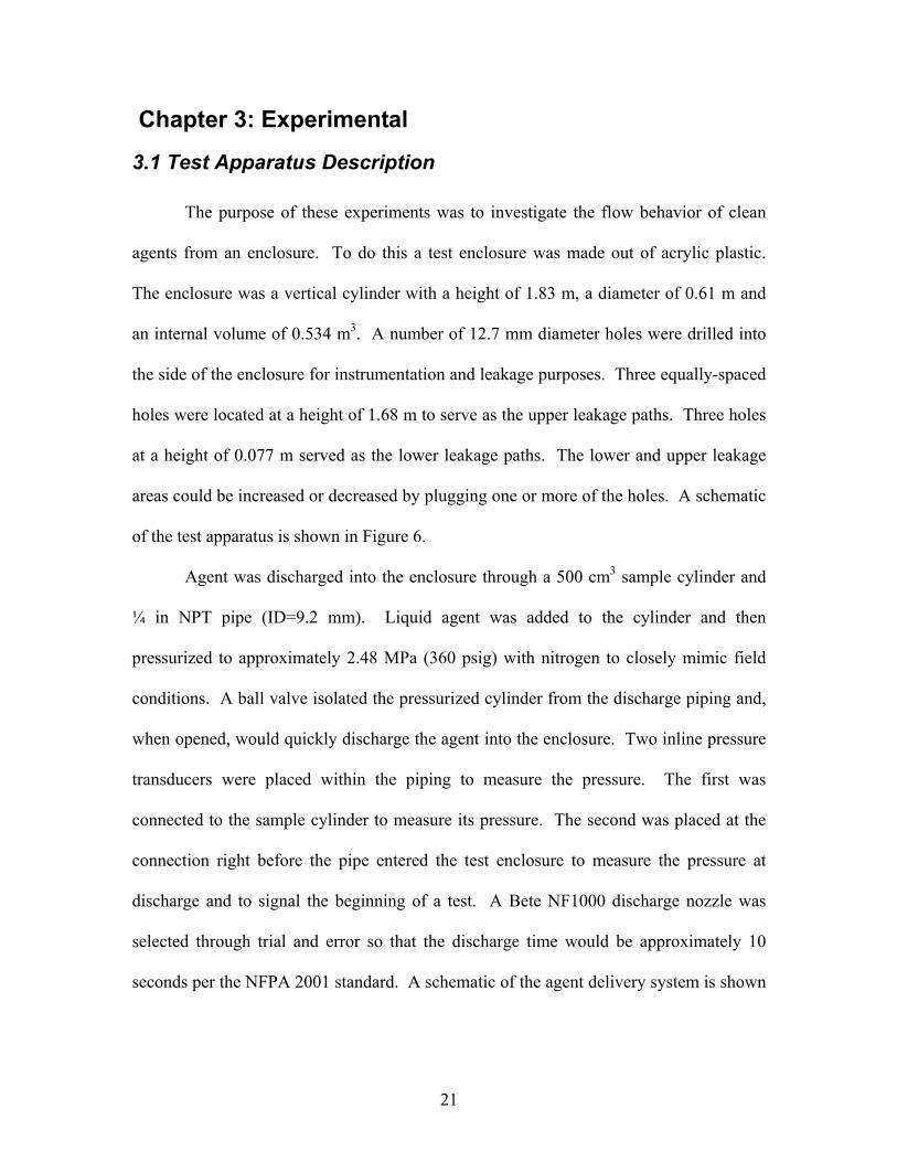
Figure 9 Agent Discharge Nozzle

25

3.2 Experimental Methodology

The design concentration for Novec 1230 is 4-6% by volume (3M Performance

Materials Division p. 3). The experiments were conducted with the high-end design

concentration of 6% for maximum flow and therefore minimum hold time. To determine

the amount of liquid agent that was needed to achieve the design concentration within the

test enclosure, Equation 15 was used, where V is the volume of the enclosure, s is the

specific volume of the superheated agent vapor, and C is the design concentration.

⎟⎠⎞

⎜⎝⎛

−=

CC

sVW

100 Equation 15 (NFPA 20001, p 2001-15)

As given in NFPA 2001 (p 2001-51), the specific volume of the Novec 1230

vapor at room temperature (25 ºC) is 0.0732575 m3/kg. Substituting these quantities into

Equation 15, it is found that 0.465 kg of Novec 1230 is required to achieve an agent

molar concentration of 6% in the test enclosure. With a liquid density of 1.6 g/m, for

Novec 1230, the volume of liquid agent needed for each experiment is 285 mL to achieve

a design concentration of 6.0%.

The required amount of liquid agent was added to the sample cylinder and all

valves were closed. The cylinder was than charged to approximately 4.8 MPa with

compressed nitrogen. The sample cylinder was shaken a number of times to allow some

nitrogen to go into solution with the liquid Novec 1230. After each shake the cylinder

was re-pressurized to 4.8 MPa. The cylinder was then reconnected to the agent delivery

system. This process was repeated approximately five times. The Tripoint analyzer and

data acquisition system were started to begin data collection. When sufficient time had

elapsed for the Tripoint Analyzer to warm-up and for baseline data to be collected, the

26

ball valve isolating the sample cylinder from the discharge piping to the enclosure was

opened and discharge occurred for approximately 10 seconds. The concentration at all

three sample ports as well as temperature and pressure differences were measured every

second for the duration of the test.

Experiments with five different area leakage scenarios were conducted to

investigate the effect of the leakage area and the leakage area ratio on the flow of the

agent-air mixture out of the enclosure. The first three sets of experiments had equal

upper and lower leakage areas of 0.00038 m2, 0.000253 m2, and 0.000127 m2

respectively. The next set of experiments had an upper leakage area of 0.00038 m2 and

lower leakage area 0.000127 m2. The final set of experiments had an upper leakage area

of 0.000127 m2 and a lower leakage area of 0.00038 m2. Table 3 summarizes the

experiments conducted.

In order to validate the leakage area scenarios presented in Table 3, the ratio of

the total leakage area to the surface area of the enclosure can be compared to that found

in actual buildings. Klote and Milke report the tightness of actual comerical buildings: an

area ratio of 0.50E10-4 as a tight bulding, 0.17E-3 as an average building, and 0.35E-3 as

a loose building. All of the experiments conducted in this project fall within the criteria

of tight or average tightness.

Table 3 Comparison of Leakage Area Scenarios

Area Leakage Scenario

# of Experiments Conducted

Ao (m2) Ai (m2) AT (m2) Area Ratio Tightness

1 3 0.00038 0.00038 0.00076 2.00E-04 Average 2 2 0.000253 0.000253 0.000506 1.33E-04 Average 3 4 0.000127 0.000127 0.000254 6.69E-05 Tight 4 2 0.000127 0.00038 0.000507 1.34E-04 Average 5 2 0.00038 0.000127 0.000507 1.34E-04 Average

27

Chapter 4 Results and Discussion

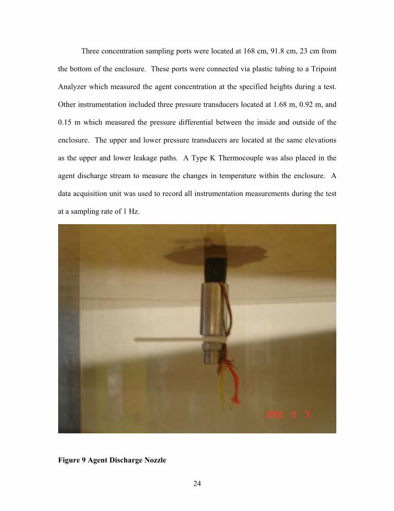
4.1 Agent Discharge

In order to closely represent an actual discharge that would occur in the field, a

discharge time of approximately 10 seconds was desired. A BETE NF1000 nozzle was

selected to meet this discharge time criteria. Evidence of the 10 second discharge time is

shown in Figure 10 with a sharp increase in pressure at the nozzle and a sharp decrease in

pressure within the agent discharge cylinder for approximately 10 seconds.

0

0.5

1

1.5

2

2.5

3

3.5

-10 -5 0 5 10 15 20

Time (s)

Pre

ssur

e (M

Pa)

CylinderNozzle

Figure 10 Inline Pressure Profiles

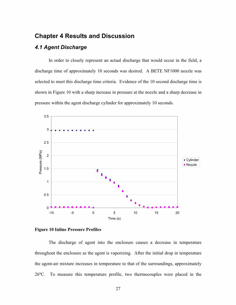
The discharge of agent into the enclosure causes a decrease in temperature

throughout the enclosure as the agent is vaporizing. After the initial drop in temperature

the agent-air mixture increases in temperature to that of the surroundings, approximately

26ºC. To measure this temperature profile, two thermocouples were placed in the

28

enclosure, one in the agent discharge stream and the other near the center of the enclosure.

Time-temperature histories generated by the thermocouples are shown in Figure 11 for

one of the experiments.

-10

-5

0

5

10

15

20

25

30

0 50 100 150 200 250 300

Time (s)

Tem

pera

ture

(°C

)

Nozzle TCenter T

Figure 11 Temperatures within the enclosure

4.2 Concentration Profiles

The primary purpose of these experiments was to evaluate how well the

theoretical model predicts the flow characteristics of the Novec 1230-air mixture out of

an enclosure. Although an agent mole fraction of approximately 6% was desired, the

measured agent mole fraction after discharge throughout the enclosure was consistently

at approximately 4.7%. This reduced mole fraction could be a result of the entire amount

of liquid agent not discharging from the sample cylinder. The Tripoint analyzer

measured the concentration at three elevations approximately every four seconds. These

29

readings provided a time-concentration profile at 1.6, 0.92, and 0.23 m within the

chamber. A set of characteristic time-concentration profiles for each set of experiments

is shown in this section. Profiles from experiments with the same leakage area conditions

as well as raw data are provided in Appendix A for all experiments.

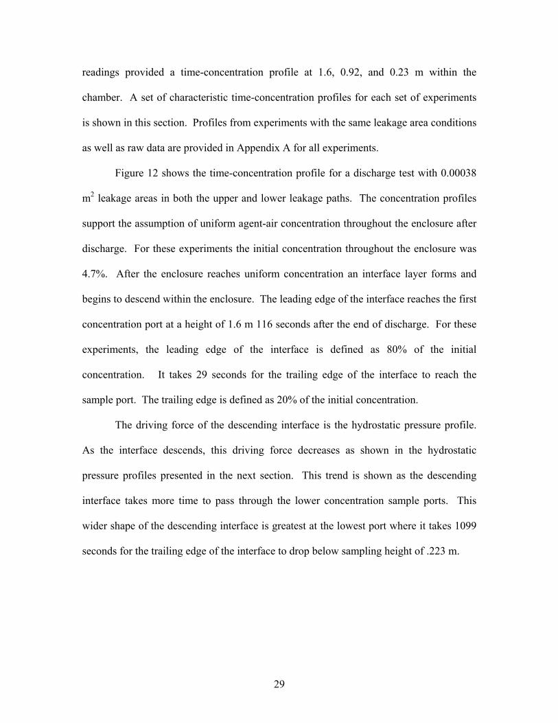
Figure 12 shows the time-concentration profile for a discharge test with 0.00038

m2 leakage areas in both the upper and lower leakage paths. The concentration profiles

support the assumption of uniform agent-air concentration throughout the enclosure after

discharge. For these experiments the initial concentration throughout the enclosure was

4.7%. After the enclosure reaches uniform concentration an interface layer forms and

begins to descend within the enclosure. The leading edge of the interface reaches the first

concentration port at a height of 1.6 m 116 seconds after the end of discharge. For these

experiments, the leading edge of the interface is defined as 80% of the initial

concentration. It takes 29 seconds for the trailing edge of the interface to reach the

sample port. The trailing edge is defined as 20% of the initial concentration.

The driving force of the descending interface is the hydrostatic pressure profile.

As the interface descends, this driving force decreases as shown in the hydrostatic

pressure profiles presented in the next section. This trend is shown as the descending

interface takes more time to pass through the lower concentration sample ports. This

wider shape of the descending interface is greatest at the lowest port where it takes 1099

seconds for the trailing edge of the interface to drop below sampling height of .223 m.

30

0

1

2

3

4

5

6

0 500 1000 1500 2000 2500 3000

Time (s)

Con

cent

ratio

n (%

)

h(t)=1.52mh(t)=0.84mh(t)=0.15m

Figure 12 Time-Concentration profile, Ao=Ai=0.00038 m2, Co=4.7%

Based on the concentration profiles observed in these experiments, it can be

assumed that the flow behavior represents that of a descending interface rather than the

continuous mixing model. However, this interface is not a sharp interface. Instead of the

profile appearing as a step-wise function, there exists a period of time where the

concentration at a given height is decreasing. This wide-interface behavior becomes

more apparent as the interface gets closer to the floor.

If the upper and lower leakage areas are equally reduced, the time-concentration

profile remains similarly shaped, but the time for the interface to reach each sample

elevation increases. Although the hydrostatic driving force remains the same, the area

available for leakage decreases, decreasing the volumetric flowrates. Figure 13 and

Figure 14 show the increased hold time for the agent to reach the respective ports as well

31

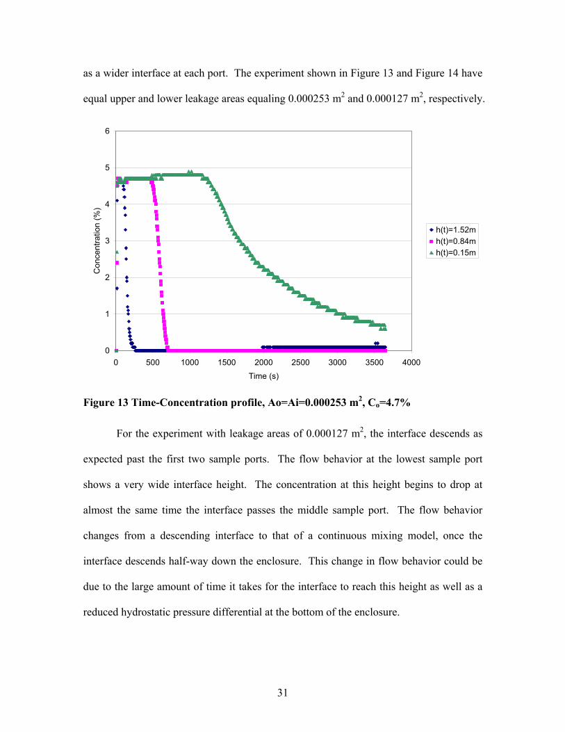
as a wider interface at each port. The experiment shown in Figure 13 and Figure 14 have

equal upper and lower leakage areas equaling 0.000253 m2 and 0.000127 m2, respectively.

0

1

2

3

4

5

6

0 500 1000 1500 2000 2500 3000 3500 4000

Time (s)

Con

cent

ratio

n (%

)

h(t)=1.52mh(t)=0.84mh(t)=0.15m


For the experiment with leakage areas of 0.000127 m2, the interface descends as

expected past the first two sample ports. The flow behavior at the lowest sample port

shows a very wide interface height. The concentration at this height begins to drop at

almost the same time the interface passes the middle sample port. The flow behavior

changes from a descending interface to that of a continuous mixing model, once the

interface descends half-way down the enclosure. This change in flow behavior could be

due to the large amount of time it takes for the interface to reach this height as well as a

reduced hydrostatic pressure differential at the bottom of the enclosure.

32

The hydrostatic pressure profile during a test is shown in Section 4.3 as Figure 19.

After approximately 1500 seconds a negative pressure difference between the inside and

outside of the enclosure develops. This negative pressure difference could allow for air

to flow into the enclosure through the lower leakage holes and create mixing of the agent-

air layer, reducing its concentration over time rather than remaining an actual descending

interface.

0

1

2

3

4

5

6

0 1000 2000 3000 4000 5000

Time (s)

Con

cent

ratio

n (%

)

h(t)=1.52mh(t)=0.84mh(t)=0.15m


For the three previous cases discussed, the upper and lower leakage areas were

equal. An experiment conducted with a leakage area ratio of 0.33 is shown in Figure 15.

With this area ratio, the leaks available for flow essentially represent unrestricted inlet

flow with restricted outlet flow. These time-concentration profiles are similar to those

33

seen in the equal area case; an interface is formed and the width of the interface increases

as the interface descends.

0

1

2

3

4

5

6

0 500 1000 1500 2000 2500 3000 3500 4000

Time (s)

Con

cent

ratio

n (%

)

h(t)=1.52mh(t)=0.84mh(t)=0.15m

Figure 15 Time-Concentration profile, Ao=0.000127 m2 Ai=0.00038 m2, Co=4.8%

Figure 16 shows an experiment with a leakage area ratio of 3. A descending

interface clearly passes the first two sample ports. However, similar to the most

restricted equal leakage area scenario (Ao=Ai=0.000127m2), the lowest concentration

sample port at a height of 0.22 m shows a time-concentration profile that would be

expected more with the continuous mixing model than a sharp descending interface.

Because of the limited inlet flow at the top of the enclosure, flow of ambient air into the

enclosure could exist at the bottom leakage holes. This entrainment of ambient air for

enclosures with large area ratios was predicted by Dewsbury and Whiteley (p. 261).

34

0

0.5

1

1.5

2

2.5

3

3.5

4

4.5

5

0 1000 2000 3000 4000 5000

Time (s)

Con

cent

ratio

n (%

)

h(t)=1.52mh(t)=0.84mh(t)=0.15m

Figure 16 Time-Concentration profile, Ao=0.00038 m2 Ai=0.000127 m2, Co=4.9%

4.3 Enclosure Pressure

The main driving force for flow out of the enclosure is the hydrostatic pressure

created by the denser agent-air mixture. When the agent is discharged into the enclosure

there is an initial decrease in the pressure while the agent is vaporizing. After this

decrease in pressure, there is an increase of pressure due to an increase in volume of the

agent-air mixture as it increases from the lower discharge temperature to that of the

surroundings (approximately 25ºC). This transient pressure behavior for the first minute

after discharge is shown in Figure 17, however these transient negative and positive

pressure spikes only occur for approximately the first 15 seconds of the test.

35

-80

-60

-40

-20

0

20

40

60

80

0 10 20 30 40 50 60

Time (s)

∆P

(Pa) h=1.68m

h=0.84mh=0 m

Figure 17 Initial Transient Hydrostatic Pressure Profile Ao=Ai=0.00038 m2,

Co=4.7%

36

After this transient behavior, typical hydrostatic pressure profiles exist at the

different heights. This behavior is shown in Figure 18. At the highest measured point

(h=1.76m) there is a negative pressure difference between the enclosure pressure and the

ambient air pressure. This pressure difference is responsible for the entrainment of the

fresh air into the enclosure. At the lowest height (h=0.077m) there exists a positive

pressure difference, forcing the agent-air mixture out of the enclosure. As the interface

layer descends, these pressure differences decrease resulting in a smaller flowrate. These

small pressure differences are responsible for the wide interface at the lowest sample port.

The small driving force, and thus flowrate, result in the interface taking more time to pass

a low height on the enclosure.

-40

-30

-20

-10

0

10

20

30

40

0 200 400 600 800 1000 1200 1400 1600

Time (s)

∆P

(Pa) h=1.68m

h=0.841mh=0m

Figure 18 Hydrostatic Pressure Differences Ao=Ai=0.00038 m2, Co=4.7%

37

-20

-15

-10

-5

0

5

10

15

20

0 1000 2000 3000 4000 5000 6000

Time (s)

∆P

(Pa) h=1.68m

h=0.841mh=0m

Figure 19 Hydrostatic Pressure Differences Ao=Ai=0.000127 m2, Co=4.7%

4.4 Dimensionless Comparison

The hold time of agent-air mixture within an enclosure is a function of the leakage

area, the density of the mixture, as well as the height of the interface. These parameters

will differ between experiments and enclosures. Therefore in order to best compare

numerous situations, the hold time should be made dimensionless. The time-

concentration data collected by the Tripoint analyzer was made dimensionless by the

equations presented in Section 2.4. Therefore all data collected could be compared to the

descending interface model.

Figure 20 shows the dimensionless descending interface (h(t)/Ho) as a function of

the dimensionless quantity k(t-to)/τ. This parameter encompasses all the experimental

parameters of each test. The experimental data reported is at the point where the

38

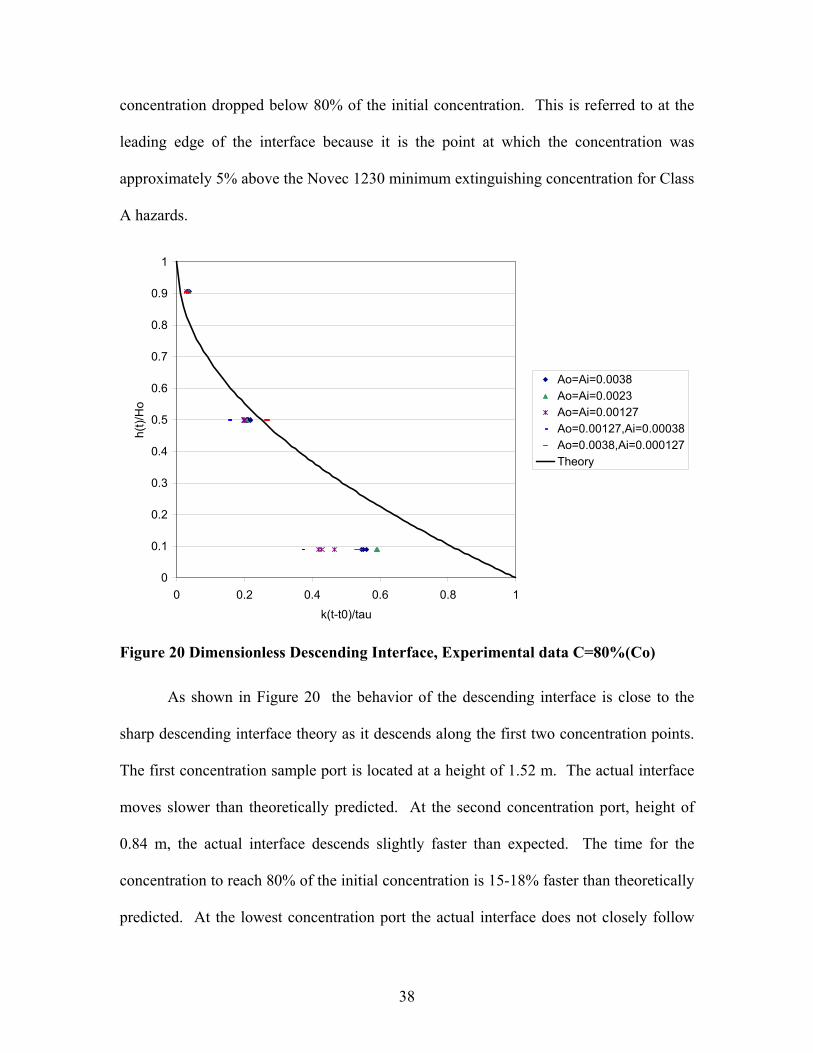
concentration dropped below 80% of the initial concentration. This is referred to at the

leading edge of the interface because it is the point at which the concentration was

approximately 5% above the Novec 1230 minimum extinguishing concentration for Class

A hazards.

0

0.1

0.2

0.3

0.4

0.5

0.6

0.7

0.8

0.9

1

0 0.2 0.4 0.6 0.8 1

k(t-t0)/tau

h(t)/

Ho

Ao=Ai=0.0038Ao=Ai=0.0023Ao=Ai=0.00127Ao=0.00127,Ai=0.00038Ao=0.0038,Ai=0.000127Theory

Figure 20 Dimensionless Descending Interface, Experimental data C=80%(Co)

As shown in Figure 20 the behavior of the descending interface is close to the

sharp descending interface theory as it descends along the first two concentration points.

The first concentration sample port is located at a height of 1.52 m. The actual interface

moves slower than theoretically predicted. At the second concentration port, height of

0.84 m, the actual interface descends slightly faster than expected. The time for the

concentration to reach 80% of the initial concentration is 15-18% faster than theoretically

predicted. At the lowest concentration port the actual interface does not closely follow

39

the descending interface model at the lowest concentration port. At this bottom location

the interface layer descends quicker than predicted by theory. The experimental

enclosure could have additional upper leakage that is not known. This additional leakage

would increase the rate of descent of the upper layer.

For comparison, the point at which the agent-air concentration reached 50% of the

initial concentration was also recorded and plotted against k(t-to)/τ. This concentration

could be considered the trailing edge of the interface and resembles concentrations below

the minimum extinguishing concentration of Novec 1230. Similar to the experimental

data the descending interface layer moves faster than predicted by theory. The model

represents the flow behavior at points greater than half of the enclosure height, but does

not favorably predict the behavior when the layer descends past this height. The time for

the concentration to reach 50% of the initial concentration for the sample port located at a

height of 0.84 m is 8-20% faster than that predicted by theory, with the exception of the

case where the lower leakage is three times that of the upper leakage. For the case where

the upper leakage is greater than the lower leakage, the layer descends slower than

predicted by theory.

40

0

0.1

0.2

0.3

0.4

0.5

0.6

0.7

0.8

0.9

1

0 0.2 0.4 0.6 0.8 1

k(t-to)/tau

h(t)/

Ho

Ao=Ai=0.0038Ao=Ai=0.0023Ao=Ai=0.00127Ao=0.00127,Ai=0.00038Ao=0.0038,Ai=0.000127Theory

Figure 21 Dimensionless Descending Interface Experimental data @ C=50%(Co)

The effect of the area ratios is also seen in these dimensionless graphs. The data

for the hold time at the uppermost port is clustered. At the middle port the experiments

with equal area are clustered while those with either restricted or increased outward flow

seem like outliers. At the bottom sample port the experimental data for a given area ratio

is clustered, but does not show similarity between experiments. Again, this lack of

similarity between experiments could be due to bidirectional flow once the descending

interface reaches heights less than half of its initial height.

41

Chapter 5: Summary and Conclusions

The main objective of this study was to evaluate the descending interface model

of the flow of fire suppression agent-air mixtures out of an enclosure. Fifteen

experiments were conducted using Novec 1230 and different leakage area scenarios. The

descending interface model proved to correctly predict the descent of the layer over the

upper half of the height of the enclosure. Below this, model under predicted the amount

of time it took for the layer to descend to a height of 0.15 m from the lower leakage

opening. The reason for the under-prediction of the hold time could be due to the

possible change in interface behavior from a sharp descending interface to a wide

interface or continuous mixing model.

Based on this investigation, the descending interface model adequately predicts

hold times to a height of approximately one-half that of the initial interface height for

agents with similar characteristics to Novec 1230. As long as the highest potential fire

source within the enclosure is in the lower half of the enclosure and the hold time is

considered the point where the interface drops to this point as stated in the NFPA 2001

standard, this model appears to be suitable for design purposes.

Further experiments with agents of different densities are needed to further

validate the descending interface model, as well as determine the agents for which this

model is valid. More concentration-time data gathered at the lower half of an enclosure

would help to better characterize the flow and interface characteristics at these heights.

The agent discharge causes negative and positive surges in internal enclosure

pressure. In order for the suppression to be effective, the enclosure needs to be able to

42

withstand these pressure surges. Further analysis of these transient pressure effects is

warranted.

.

43

Appendix A: Raw Data and Supplemental Graphs

A total of 13 experiments were run with five different leakage area conditions.

Table A-1 outlines the experiment name, leakage areas, initial concentration, densities,

and the calculated parameters k2 and t used in the dimensionless comparison.

Table A-1 Experimental Raw Data

Experiment Ao (m2) Ai (m2) Co (%) ρo

(kg/m3) ρm

(kg/m3) k2 τ t(Ho/2)pre

(s) 072805_Test2 0.00038 0.00038 5.5 0.168 1.855 0.337 521.48 453.24 080105_Test1 0.00038 0.00038 4.6 0.168 1.742 0.314 521.48 486.30 080305_Test1 0.00038 0.00038 4.7 1.168 1.755 0.317 521.48 482.13

080305_Test2 0.000253 0.000253 4.7 1.168 1.755 0.317 782.22 723.19 080305_Test6 0.000253 0.000253 4.75 1.168 1.761 0.318 782.22 720.14

080305_Test3 0.000127 0.000127 4.8 1.168 1.767 0.319 1564.44 1434.29 080305_Test5 0.000127 0.000127 4.6 1.168 1.742 0.314 1564.44 1458.89 080505_Test1 0.000127 0.000127 4.7 1.168 1.755 0.317 1564.44 1446.38 080505_Test3 0.000127 0.000127 4.75 1.168 1.761 0.318 1564.44 1440.28

080405_Test2 0.000127 0.00038 4.8 1.168 1.767 0.397 1564.44 1153.04 080405_Test3 0.000127 0.00038 4.8 1.168 1.767 0.397 1564.44 1153.04

080405_Test4 0.00038 0.000127 4.3 1.168 1.705 0.148 521.48 1030.54 080405_Test5 0.00038 0.000127 4.9 1.168 1.780 0.158 521.48 968.34

The Tripoint Analyzer gathered concentration data at heights of 1.52, 0.841, and

0.151 m. The time at which the concentration at the sample height reached 80, 20, and

50% of the initial concentration was recorded and is reported in Table A-2. For these

data, time zero is the time at which discharge began.

44

Table A-2 Interface concentration-time data collected by Tripoint Analyzer.

Ao=Ai=0.00038 Time for concentration to reach

Experiment h(t) 80% (Co) 50% (Co) 20% (Co) ∆t 072805_Test2 1.52 102 113 136 34

0.841 384 413 452 68 0.151 290 1016 1260 970

080105_Test1 1.52 97 112 126 29 0.841 394 418 457 63 0.151 958 1094 1464 506

080305_Test1 1.52 97 107 126 29 0.841 394 418 447 53 0.151 968 1099 2417 1449


h(t) 80% (Co) 50% (Co) 20% (Co) ∆t 080305_Test2 1.52 131 175 44 146

0.841 554 651 97 603 0.151 1503 3108 1605 1931

080305_test6 1.52 131 146 185 1931 0.841 550 593 647 1931 0.151 1498 1926 3239 1931



0.841 1017 1143 1299 282 0.151 2325 3424 5715 3390

080305_Test5 1.52 195 229 272 77 0.841 1036 1153 1308 272 0.151 2179 3307 5326 3147

080305_Test1 1.52 190 219 277 87 0.841 1041 1167 1313 272 0.151 2106 3191 4995 2889

Ao=0.000127, Ai=0.00038 Time for concentration to reach


0.841 652 705 759 107 0.151 1503 1707 2340 837

080405_Test3 1.52 175 195 229 54 0.841 657 705 764 107 0.151 1503 1697 2471 968

45

Ao=0.00038, Ai=0.000127 Time for concentration to reach


0.841 978 119 1284 306 0.151 1916 3040 4898 2982

080405_Test5 1.52 146 175 263 117 0.841 929 1060 1206 277 0.151 1834 3040 4835 3001

The following graphs show the hydrostatic pressure profiles as well as the time-

concentration profiles for all experiments. The pressure data was collected at h(t) heights

1.68, .841, and 0 m and the concentration data was collected at h(t) heights of 1.52, 0.84,

and 0.15 m respectively.

46

-80

-60

-40

-20

0

20

40

60

80

0 500 1000 1500 2000 2500 3000

Time (s)

∆P

(Pa) PT1

PT2PT3

Figure A 1:Experiment 072805_Test 2 Pressure Profiles Ao=Ai=0.00038 m2

0

1

2

3

4

5

6

0 500 1000 1500 2000

Time (s)

Con

cent

ratio

n (%

)

Conc 1Conc 2Conc 3

Figure A 2: Experiment 072805_Test 2 Concentration Profiles Ao=Ai=0.00038 m2

47

-40

-30

-20

-10

0

10

20

30

40

0 200 400 600 800 1000 1200 1400 1600

Time (s)

∆P

(Pa) h=1.68m

h=0.841mh=0m

Figure A 3: Experiment 080105_Test1 Pressure Profiles Ao=Ai=0.00038 m2

0

1

2

3

4

5

6

0 500 1000 1500 2000

Time (s)

Con

cent

ratio

n (%

)

Conc 1Conc 2Conc 3

Figure A 4 Experiment 080105_Test1 Concentration Profiles Ao=Ai=0.00038 m2

48

-20

-15

-10

-5

0

5

10

15

20

0 500 1000 1500 2000 2500 3000

Time (s)

∆P

(Pa) h=1.68m

h=.84mh=0m

Figure A 5 Experiment 080305_Test1 Pressure Profiles Ao=Ai=0.00038 m2

0

1

2

3

4

5

6

0 500 1000 1500 2000 2500 3000

Time (s)

Con

cent

ratio

n (%

)

h(t)=1.52mh(t)=0.84mh(t)=0.15m


49

-80

-60

-40

-20

0

20

40

60

80

0 500 1000 1500 2000

Time (s)

DP

(Pa) PT1

PT2PT3


0

1

2

3

4

5

6

0 500 1000 1500 2000 2500 3000 3500 4000Time (s)

Con

cent

ratio

n (%

)

h(t)=1.52mh(t)=0.84mh(t)=0.15m


50

-80

-60

-40

-20

0

20

40

60

80

0 1000 2000 3000 4000

Time (s)

DP

(Pa) PT1

PT2PT3


0

1

2

3

4

5

6

0 500 1000 1500 2000 2500 3000 3500 4000Time (s)

Con

cent

ratio

n (%

)

Conc 1Conc 2Conc 3


51

-40

-30

-20

-10

0

10

20

30

40

0 1000 2000 3000 4000 5000 6000

Time (s)

∆P

(Pa) h=1.68m

h=0.841mh=0m


0

1

2

3

4

5

6

0 1000 2000 3000 4000 5000 6000 7000Time (s)

Con

cent

ratio

n (%

)

Conc 1Conc 2Conc 3


52

-80

-60

-40

-20

0

20

40

60

80

0 1000 2000 3000 4000 5000

Time (s)

DP

(Pa) PT1

PT2PT3


0

1

2

3

4

5

6

0 1000 2000 3000 4000 5000Time (s)

Con

cent

ratio

n (%

)

h(t)=1.52mh(t)=0.84mh(t)=0.15m


53

-80

-60

-40

-20

0

20

40

60

80

0 1000 2000 3000 4000 5000

Time (s)

DP

(Pa) PT1

PT2PT3


0

1

2

3

4

5

6

0 1000 2000 3000 4000 5000Time (s)

Con

cent

ratio

n (%

)

Conc 1Conc 2Conc 3


54

-40

-30

-20

-10

0

10

20

30

40

0 1000 2000 3000 4000 5000 6000

Time (s)

DP

(Pa) h=1.68m

h=0.841h=0


0

1

2

3

4

5

6

0 500 1000 1500 2000 2500 3000 3500 4000Time (s)

Con

cent

ratio

n (%

)

Conc 1Conc 2Conc 3


55

-80

-60

-40

-20

0

20

40

60

80

0 500 1000 1500 2000 2500 3000 3500

Time (s)

DP

(Pa) PT1

PT2PT3

Figure A 19 Experiment 080405_Test2 Pressure Profiles Ao=0.000127 m2 Ai=0.00038 m2

0

1

2

3

4

5

6

0 500 1000 1500 2000 2500 3000 3500 4000

Time (s)

Con

cent

ratio

n (%

)

h(t)=1.52mh(t)=0.84mh(t)=0.15m

Figure A 20 Experiment 080405_Test2 Pressure Profiles Ao=0.000127 m2 Ai=0.00038 m2

56

:

-80

-60

-40

-20

0

20

40

60

80

0 500 1000 1500 2000 2500 3000 3500 4000

Time (s)

DP

(Pa) PT1

PT2PT3

Figure A 21: Experiment 080305_Test2 Pressure Profiles Ao=0.000127 m2

Ai=0.00038 m2

0

1

2

3

4

5

6

0 500 1000 1500 2000 2500 3000 3500 4000

Time (s)

Con

cent

ratio

n (%

)

Conc 1Conc 2Conc 3

Figure A 22 Experiment 080305_Test2 Concentration Profiles Ao=0.000127 m2

Ai=0.00038 m2

57

0

0.5

1

1.5

2

2.5

3

3.5

4

4.5

5

0 1000 2000 3000 4000 5000

Time (s)

Con

cent

ratio

n (%

)

h(t)=1.52mh(t)=0.84mh(t)=0.15m


Ai=0.000127 m2

58

-20

-15

-10

-5

0

5

10

15

20

0 1000 2000 3000 4000 5000

Time (s)

∆P

(Pa) PT1

PT2PT3

Figure A 24 Experiment 080405_Test5 Pressure Profiles Ao=0.00038 m2

Ai=0.000127 m2

0

1

2

3

4

5

6

0 1000 2000 3000 4000 5000Time (s)

Con

cent

ratio

n (%

)

h(t)=1.6mh(t)=0.92mh(t)=0.22m


Ai=0.00038 m2

59

Appendix B: Pressure Transducer Calibration Curves

Three pressure transducers were placed at h(t) heights of 1.68, 0.84, and 0 m to

measure the hydrostatic pressure differences between the inside and outside of the

enclosure. After the initial pressure surges, these pressure differences ranged from 0-20

PA. Due to the small pressure variations it is important that the pressure transducers are

correctly calibrated. The calibration curves for the pressure transducers are shown below.

Pressure transducer 2628046 h=1.68 m

y = 49.716x - 126.7R2 = 1

-150

-100

-50

0

50

100

150

0 0.5 1 1.5 2 2.5 3 3.5 4 4.5 5

Voltage (VDC)

Pre

ssur

e di

ffere

ntia

l (Pa

)

Cal. dataLinear (Cal. data)

60

Pressure transducer 2628047 h=0.84 m

y = 49.838x - 126.72R2 = 1

-150

-100

-50

0

50

100

150

0 0.5 1 1.5 2 2.5 3 3.5 4 4.5 5

Voltage (VDC)

Pre

ssur

e di

ffere

ntia

l (Pa

)

Cal. dataLinear (Cal. data)

61

References

3M, “Novec 1230 Brochure”, 3M Specialty Materials Division, 2003

http://www.3m.com/novec1230fluid

Dewsbury J., and Whiteley, R. A., “Extensions to standard hold time calculations,” Fire

Technology, Vol. 36, No. 4, 2000, pp 266- 278.

Dewsbury J., and Whiteley, R. A., “Review of fan integrity testing and hold time

standards,” Fire Technology, Vol. 36, No. 4, 2000, pp 249- 265.

Dewsbury J., and Whiteley, R. A., “Hold time calculations for non-standard enclosures,”

Fire Technology, Vol. 40, 2004, pp 78-89.

DiNenno, P., Halon Replacement Clean Agent Total Flooding Systems The SFPE

Handbook of Fire Protection Engineering 3rd Ed, Society of Fire Protection

Engineers, 2002 pp 4-173-4-198.

DiNenno, P. J., and Forssell, E. W. “Evaluation of the door fan pressurization leakage

test method applied to Halon 1301 total flooding systems,” Journal of Fire

Protection Engineering, Vol. 1, No. 4, 1989, pp 131-140.

ISO/fDIS 1450.1 Gaseous fire extinguishing systems – Physical properties and system

design, Part 1: General Requirements, Annex E, International Standards

Organization, 2003.

Klocke, M., Door-fan-test Proceedings of Congress on Fire Extinguishing Systems, VdS,

Cologne, Germany, December 1998.

Myint L.S., Methodologies for limiting emissions of halogenated fire extinguishant

agents for enclosures, Ph.D. thesis, University of Manchester Faculty of

Technology (UMIST), Manchester, England ,1991.

NFPA 2001, Standard on clean agent fire extinguishing systems, National Fire Protection

Association, 2004

Date post:	03-Feb-2022
Category:	Documents
Upload:	others
View:	2 times
Download:	0 times

ABSTRACT Title: ANALYSIS OF HOLD TIMES FOR GASEOUS FIRE

Documents