Research Note RN/13/17 Learning Combinatorial Interaction Testing Strategies using Hyperheuristic Search September 17, 2013 Yue Jia Myra B. Cohen Mark Harman Justyna Petke Abstract Two decades of bespoke Combinatorial Interaction Testing (CIT) algorithm development have left software engineers with a bewildering choice of configurable system testing techniques. This paper introduces a single hyperheuristic algorithm that earns CIT strategies, providing a single generalist approach. We report experiments that show that our algorithm competes with known best solutions across constrained and unconstrained problems. For all 26 real world subjects and 29 of the 30 constrained benchmark problems studied, it equals or improves upon the best known result. We also present evidence that our algorithm's strong generic performance is caused by its effective unsupervised learning. Hyperheuristic search is thus a promising way to relocate CIT design intelligence from human to machine. UCL DEPARTMENT OF COMPUTER SCIENCE
Transcript
Research Note RN/13/17
Learning Combinatorial Interaction Testing Strategies using Hyperheuristic
Search
September 17, 2013
Yue Jia
Myra B. Cohen
Mark Harman
Justyna Petke
Abstract Two decades of bespoke Combinatorial Interaction Testing (CIT) algorithm development have left software engineers with a bewildering choice of configurable system testing techniques. This paper introduces a single hyperheuristic algorithm that earns CIT strategies, providing a single generalist approach. We report experiments that show that our algorithm competes with known best solutions across constrained and unconstrained problems. For all 26 real world subjects and 29 of the 30 constrained benchmark problems studied, it equals or improves upon the best known result. We also present evidence that our algorithm's strong generic performance is caused by its effective unsupervised learning. Hyperheuristic search is thus a promising way to relocate CIT design intelligence from human to machine.
ABSTRACTTwo decades of bespoke Combinatorial Interaction Test-ing (CIT) algorithm development have left software engi-neers with a bewildering choice of configurable system test-ing techniques. This paper introduces a single hyperheuris-tic algorithm that learns CIT strategies, providing a singlegeneralist approach. We report experiments that show thatour algorithm competes with known best solutions acrossconstrained and unconstrained problems. For all 26 realworld subjects and 29 of the 30 constrained benchmark prob-lems studied, it equals or improves upon the best known re-sult. We also present evidence that our algorithm’s stronggeneric performance is caused by its e↵ective unsupervisedlearning. Hyperheuristic search is thus a promising way torelocate CIT design intelligence from human to machine.
Categories and Subject DescriptorsD.2.5 [Software Engineering]: Testing and Debugging
1. INTRODUCTIONCombinatorial Interaction Testing (CIT) is important be-
cause of the increasing reliance on configurable systems. CITaims to generate samples that cover all possible value com-binations between any set of t parameters, where t is fixed(usually between 2 and 6). Software product lines, operatingsystems, development environments and many other systemsare typically governed by large configuration parameter andfeature spaces for which CIT has proved useful [30].
Permission to make digital or hard copies of all or part of this work for
personal or classroom use is granted without fee provided that copies are
not made or distributed for profit or commercial advantage and that copies
bear this notice and the full citation on the first page. To copy otherwise, to
republish, to post on servers or to redistribute to lists, requires prior specific
permission and/or a fee.
ICSE 2014, India
Copyright 20XX ACM X-XXXXX-XX-X/XX/XX ...$15.00.
Over two decades of research has gone into the develop-ment of bespoke CIT test generation techniques, each ofwhich is tailored and tuned to a specific problem. For ex-ample, some CIT algorithms have been tuned and evalu-ated only on unconstrained problems [8, 12, 24, 27], whileothers have been specifically tuned for constrained interac-tion testing [4, 19], which prohibits certain configurations.Still other CIT approaches target specific problem struc-tures, such as parameter spaces with few available parame-ter value choices [28,31], or are tuned to work on a particularset of real world problems [36].
The tester is therefore presented with many di↵erent tech-niques and implementations from which to choose, each ofwhich has its own special properties. Unfortunately, thischoice can be a bewildering one, because an algorithm de-signed for one CIT instance may perform poorly when ap-plied to another (or may even be inapplicable). It may notbe reasonable to expect a practicing software tester to per-form their own experiments to decide on the best CIT algo-rithm choice for each and every testing problem. It wouldbe equally unreasonable to expect every organisation to hirean algorithm designer to build bespoke CIT testing imple-mentations for each testing scenario the organisation faces.
To overcome some of the practical di�culties in choos-ing among available implementations, there has been an at-tempt to collate algorithms into a common framework with asingle unified interface [6]. This framework seeks to ensurethat all implementations ought to be at least easily appli-cable. However, it cannot help the tester to choose whichalgorithm to apply to each CIT problem instance. Instead,he or she must run experiments to gather this data.
To address this problem we introduce a simulated anneal-ing hyperheuristic search based algorithm. Hyperheuristicsare a new class of Search Based Software Engineering al-gorithms, the members of which use dynamic adaptive op-timisation to learn optimisation strategies without supervi-sion [3, 22]. Our hyperheuristic algorithm learns the CITstrategy to apply dynamically, as it is executed. This singlealgorithm can be applied to a wide range of CIT probleminstances, regardless of their structure and characteristics.
For our new algorithm to be acceptable as a generic so-lution to the CIT problem, we need to demonstrate that itis e↵ective and e�cient across a wide range of CIT prob-lem instances, when compared to other possible algorithmchoices. To assess the e↵ectiveness of CIT solutions we usethe size of the final sample.
1
Garvin et al. [19] have demonstrated that this size hasthe greatest impact on the overall e�cacy of CIT. To assesse�ciency we report computational time (as is standard inCIT experiments), but we also deploy the algorithms in thecloud. Cloud deployment provides an unequivocal supple-mental assessment of monetary cost (as has been done inrecent software engineering studies [25]).
We compare our hyperheuristic algorithm, not only againstresults from other state-of-the-art CIT techniques, but alsoagainst the best known results in the literature, garneredover 20 years of analysis of CIT. This is a particularly chal-lenging ‘quality comparison’ for any algorithm, because someof these best known results are the product of many yearsof careful analysis by mathematicians, not machines.
We show that our hyperheuristic algorithm performs wellon both constrained and unconstrained problems and acrossa wide range of parameter sizes and data sets that includesboth two and three-way coverage. Like the best knownresults, some of these data sets have been designed usinghuman ingenuity. Human design ensures that these bench-marks capture especially pathological ‘corner cases’ and prob-lems with specific structures that are known to pose chal-lenges to the CIT algorithms.
Overall, our results provide evidence to support the claimthat hyperheuristic search is a promising solution to CIT,potentially replacing the current bewildering range of choiceswith a single, generic solution that learns to tailor itself tothe configuration testing problem to which it is applied.
The primary contributions of this paper are:
1. The formulation of CIT as a hyperheuristic search prob-lem and the introduction of the first hyperheuristic al-gorithm for solving this problem. This work is alsothe first use of hyperheuristic learning in the SoftwareEngineering literature.
2. A comprehensive empirical study showing that thisapproach is both e↵ective and e�cient. The studyreports results across a wide range of 59 previouslystudied benchmarks that include known pathologicaland corner cases. We also study 26 problem instancesfrom two previous studies where each of the 26 CITproblems is drawn from a real world configurable sys-tem testing problem. These study subjects cover bothconstrained and unconstrained CIT problems, and wereport results for both 2-way and 3-way interactioncoverage for a subset of these.
3. We use the Amazon EC2 cloud to measure the realcomputational cost (in US dollars) of the algorithmsstudied. These results indicate that, with default set-tings, our hyperheuristic algorithm can produce com-petitive results to state-of-the-art tools at a reasonablecost. For example, our algorithm produces all the pair-wise interaction tests reported in the paper for all 26real world problems and the 44 pairwise benchmarksfor a total cost of only $2.09.
4. A further empirical study is used to explore the natureof online learning employed by our algorithm. The re-sults of this study show that the hyperheuristic searchproductively combines heuristic operators that wouldhave proved to be unproductive in isolation. Our re-sults also demonstrate how the hyperheuristic adaptsits choice of operators to the specific problem to whichit is applied.
2. PRELIMINARIESIn this section we will give a quick overview of the nota-
tion used throughout the paper. CIT produces a CoveringArray (CA), which is typically represented as follows in theliterature:
CA(N ; t, vk11 v
k22 ...v
kmm )
where N is the size of the array, the sum of k1, ..., km isthe number of parameters (or factors), each vi stands forthe number of values for each of the ki parameters in turnand t is the strength of the array; a t-way interaction testsuite aims to cover all possible t-way combinations of valuesbetween any t parameters.
Suppose we want to generate a pairwise (aka 2-way) in-teraction test suite for an instance with 3 parameters, wherethe first and third parameter can take 4 di↵erent values andthe second one can only take 3 di↵erent values. Then theproblem can be formulated as: CA(N ; 2, 413141) and themodel of the problem is 413141.
Furthermore, in order to test all combinations one wouldneed 4 ⇤ 3 ⇤ 4 = 48 test cases, pairwise coverage reducesthis number to 16. Suppose that we have the following con-straints: only the first value for the first parameter can everbe combined with values for the other parameters, and thelast value for the second parameter can never be combinedwith values for all the other parameters. Introducing theseconstraints reduces the size of the test suite further; only8 test cases are now required to cover all feasible interac-tions. Since constraints reduce test suite size and naturallyoccur in real-world problems, constrained CIT is well-fittedfor industrial applications [33].
Many di↵erent algorithms have been introduced to gener-ate covering arrays. Each of these algorithms is customisedfor specific problem instances. For example, there have beengreedy algorithms, such as the Automatic E�cient Test CaseGenerator, AETG [8] , the ‘In Parameter Order’ algorithm(IPO) [26] and PICT [15]. These methods either generate anew test case on-the-fly, seeking to cover the largest numberof uncovered t-way interactions, or start with a small num-ber of parameters and iteratively add new columns and rowsto fill in the missing coverage.
Other approaches include metaheuristic search algorithms,such as simulated annealing [12, 19, 28] or tabu search [31].These metaheuristics are usually divided into two phases orstages. In the first stage, binary search, for instance, is usedto generate a random test suite, r of fixed size n. In the sec-ond stage, metaheuristic search is used to search for a testsuite of size n, starting with r, that covers as many inter-actions as possible. And there are other unique algorithms,such as those that use constraint solving or logic techniquesas the core of their approach [6, 24].
3. HYPERHEURISTIC CIT ALGORITHMHyperheuristic search is a new class of optimisation al-
gorithms for Search Based Software Engineering [21]. Hy-perheuristics have been successfully applied to many opera-tional research problems outside of software engineering [3].However, though they have been advocated as a possiblesolution to dynamic adaptive optimisation for software en-gineering [22], they have not, hitherto, been applied to anysoftware engineering problem [1,23,34]. There are two sub-classes of hyperheuristic algorithms: generative and selec-tive. Generative hyperheuristics combine low level heuristicsto generate new higher level heuristics.
2
Selective hyperheuristics select from a set of low levelheuristics. In this paper we use a selective hyperheuristicalgorithm. Selective hyperheuristic algorithms can be fur-ther divided into two classes, depending upon whether theyare online or o✏ine. We use online selective hyperheuris-tics, since we want a solution that can learn to select thebest CIT heuristic to apply, unsupervised, as it executes.
The hyperheuristic algorithm takes the set of lower levelheuristics as input, and layers the heuristic search into twolevels that work together to produce the overall solution.The first (or outer) layer uses a normal metaheuristic searchto find solutions directly from the solution space of the prob-lem. The inner layer heuristic, searches for the best candi-date lower heuristics for the outer layer heuristics in thecurrent problem state. As a result, the inner search adap-tively identifies and exploits di↵erent strategies according tothe characteristics of the problems it faces.
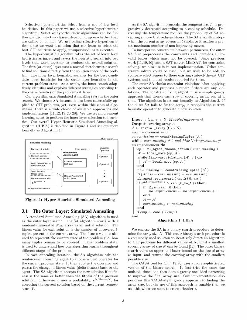
Our algorithm uses Simulated Annealing (SA) as the outersearch. We choose SA because it has been successfully ap-plied to CIT problems, yet, even within this class of algo-rithms, there is a wide choice of available approaches andimplementations [11, 12, 19, 20, 28]. We use a reinforcementlearning agent to perform the inner layer selection to heuris-tics. Our overall Hyper Heuristic Simulated Annealing al-gorithm (HHSA) is depicted in Figure 1 and set out moreformally as Algorithm 1.
Simulated Annealing
Outer search
Get next operator
Apply the operator to current solution
Send the delta fitness value
Reinforcement Learning Agent
Inner search
Operator SelectionSoft max
Reward AssignmentAction value
Random init solution Navigation Operators
Operator 1
Operator 2
Operator 3
. . .
Update solution with
Update temperature
fitness / T e
Figure 1: Hyper Heuristic Simulated Annealing
3.1 The Outer Layer: Simulated AnnealingA standard Simulated Annealing (SA) algorithm is used
as the outer layer search. The SA algorithm starts with arandomly generated Nxk array as an initial solution. Thefitness value for each solution is the number of uncovered t-tuples present in the current array. The fitness value is alsoused to represent the current state of the problem (i.e. howmany tuples remain to be covered). This ‘problem state’is used to understand how our algorithm learns throughoutdi↵erent stages of the problem.
In each annealing iteration, the SA algorithm asks thereinforcement learning agent to choose a best operator forthe current problem state. It then applies the operator andpasses the change in fitness value (delta fitness) back to theagent. The SA algorithm accepts the new solution if its fit-ness is the same or better than the fitness of the previoussolution. Otherwise it uses a probability, e
�fitness/T , foraccepting the current solution based on the current temper-ature T .
As the SA algorithm proceeds, the temperature, T , is pro-gressively decreased according to a cooling schedule. De-creasing the temperature reduces the probability of SA ac-cepting a move that reduces fitness. The SA algorithm stopswhen the current array covers all t-tuples or it reaches a pre-set maximum number of non-improving moves.
To incorporate constraints between parameters, the outerSA first preprocesses the constraints and identifies all in-valid tuples which must not be covered. Since previouswork [11,19,20] used a SAT-solver, MiniSAT, for constraintsolving, we also use it in our implementation. Other con-straint solvers could be used, but we wish to be able tocompare e↵ectiveness to these existing state-of-the-art CITsystems and the best results reported for them.
The outer SA checks constraint violations after applyingeach operator and proposes a repair if there are any vio-lations. The constraint fixing algorithm is a simple greedyapproach that checks each row of covering array, one at atime. The algorithm is set out formally as Algorithm 2. Ifthe outer SA fails to fix the array, it reapplies the currentheuristic operator to generate a new solution.
Input : t, k, v, c, N, MaxNoImprovment
Output: covering array A
A initial_array (t,k,v,N)no improvement 0curr missing countMissingTuples (A )while curr missing 6= 0 and MaxNoImprovment 6=no improvement do
op rl_agent_choose_action ( curr missing )A
0 = local_move (op, A )while fix_cons_violation (A0, c ) do
A
0 = local_move (op, A )endnew missing countMissingTuples (A0 )�fitness = curr missing � new missing
rl_agent_set_reward ( op, �fitness )if e
�fitness/Temp> rand_0_to_1 () then
if �fitness = 0 thenno improvement no improvement + 1
endA A
0
curr missing new missing
endTemp cool ( Temp )
endAlgorithm 1: HHSA
We enclose the SA in a binary search procedure to deter-mine the array size N . This outer binary search procedure isa commonly used solution to iteratively direct an algorithmto CIT problems for di↵erent values of N , until a smallestcovering array of size N can be found [12]. The outer binarysearch takes an upper and lower bound on the size of arrayas input, and returns the covering array with the smallestpossible size.
The CASA tool for CIT [19,20] uses a more sophisticatedversion of the binary search. It first tries the same sizemultiple times and then does a greedy one sided narrowingto improve the final array size. Our implementation alsoperforms this ‘CASA-style’ greedy approach to finding thearray size, but the use of this approach is tunable (i.e. weuse this when we want to search ‘harder’).
3
Input : constraints c, row R
Output: has violation
has violation False
fix time 0recheck: foreach clause in c do
foreach term in clause doif R has term then
has violation True
elsehas violation False
break
endendif has violation then
if fix time = MaxFixT ime thenbreak
endterm =clause_get_random_term (clause )R = random_fix_term (R, term )fix time = fix time +1go to recheck
endend
Algorithm 2: Constraint Violation Fixing
3.2 The Reinforcement Learning AgentThe goal of the inner layer is to select the best operator at
the current problem state. This operator selection problemcan be considered an n-Armed Bandit Problem, in which then arms are the n available heuristics and the machine learnerneeds to determine which of these heuristics o↵ers the bestreward at each problem state. We designed a ReinforcementLearning (RL) agent for the the inner search, as RL agentsare known to provide generally good solutions to this kindof so-called ‘Bandit Problem’ [38].
As shown in Figure 1, the RL agent takes a set of oper-ators as input. In each annealing iteration, the RL agentrepeatedly chooses the best fit operator, a, based on the ex-pected reward of applying operators at current state of theproblem.
After applying the operator a, the RL agent receives areward value from the outer layer SA algorithm, based onperformance. At the end of the iteration, the RL agentupdates the expected reward for the chosen operator withthe reward value returned.
The goal of the RL agent is to maximise the expectedtotal reward that accrues over the entire running time ofthe algorithm. Because the reward returned by SA is theimprovement of SA’s fitness value, the RL agent will thus‘learn’ to choose the operators that tend to maximise theSA’s fitness improvement, adapting to changes in problemcharacteristics.
Our RL agent uses an action-value method [38] to estimatethe expected rewards for each of the operators available toit at a given problem state. That is, given a set of opera-tors A = {a1, a2, . . . , ai}, let Ri = {ri1, ri2, . . . , rik}, be thereturned reward values of operator ai at the k
th iteration atwhich ai is applied.The estimated reward ai is defined as the mean reward
value, ri1+ri2+···+rikka
, received from SA. We balance the twinlearning objectives of exploration and exploitation, the RLagent uses a softmax selection rule [38].
The softmax selection rule is a greedy approach thatgives the operator with the best estimated reward the high-est selection probability. For each operator ai, the selec-tion probability is defined based on the Gibbs distribution:
eRai/T
Pnj=1 e
Raj /T . A higher value of temperature T makes the se-
lection of all operators more equal while a lower value makesa greater di↵erence in selection probability.
3.3 Search Space Navigation OperatorsWe have selected a set of six operators to investigate the
performance and feasibility of this approach to adaptivelearning for CIT. Like any general process, we choose op-erators that can be widely applicable and which the learnermight be able to combine in productive ways. Since we mustbe general, we cannot exploit specific problem characteris-tics, leaving it to the learner to find ways to do this throughthe smart combination of the low level heuristics we define.
We have based our operator selection on the previous algo-rithms for CIT. None of the operators considers constraintsdirectly, but some have been used for constrained and somefor unconstrained problems. Like other machine learningapproaches we need a combination of ‘smart’ heuristic and‘standard’ heuristics, since each can act as an enabler forthe other. The first three operators are ones we deem tobe entirely standard; they do not require book keeping orsearch for particular properties before application. The sec-ond set are ones that we deem to be somewhat smart; theseuse information that one might expect could potentially helpguide the outer search. The operators are as follows:
1. Single Mutation (Std): Randomly select a row r anda column c, change the value at r, c to a random validvalue. This operator matches the neighbourhood trans-formation in the unconstrained simulated annealing al-gorithm [12].
2. Add/Del: (Std): Randomly delete a row r and add anew row r
0 randomly generated. While CASA includesa row replacement operator, that one uses intelligence(i.e. the row is not just randomly generated).
3. Multiple Mutation (Std): Randomly select two rows,r1 and r2, and crossover each column of r1 and r2 witha probability of 0.2.
4. Single Mutation (Smart): Randomly select a miss-ing tuple, m, which is the combination of columnsc1, . . . , cn. Go through each row in the covering ar-ray, if there exists a duplicated tuple constructed bythe same combination of columns c1, . . . , cn, find a rowcontaining the duplication randomly and change therow to cover the missing tuple m. Otherwise randomlyselect a row r and change the row to cover the missingtuple m.
5. Add/Del: (Smart): Randomly delete a row r, and adda new row r
0 to cover n missing tuples. We define n asthe smaller value from k/2 (where k is the number ofparameters) and the number of missing tuples. Thisis a simple form of constructing a new row used byAETG [8].
6. Multiple Mutation (Smart): Randomly select two rows,r1 and r2, and compare the frequency of a value at eachcolumn, fc1 and fc2. With probability of 0.2, the col-umn with high frequency will be mutated to a randomvalue.
4
4. EXPERIMENTSIn order to assess the usefulness of using our hyperheuris-
tic algorithm as a general approach to CIT, we built ourversion of the hyperheuristic simulated annealing algorithmand posed the following research questions:1
RQ1 What is the quality of the test suites generatedusing the hyperheuristic approach?
One of the primary goals of CIT is to find the smallesttest suite (defined by the covering array) that achieves thedesired strength coverage. It is trivial to generate an ar-bitrarily large covering test suite - simply include one testcase for each interaction to be covered. However, such anaıve approach to test generation would yield exponentiallymany test cases. All CIT approaches therefore work aroundproblem of finding a minimal size covering array for testing.The goal of CIT is to try to find the smallest test suite thatachieves 100% t-way interaction coverage for some chosenstrength of interaction t. In our experiment, we comparethe size of the test suites generated by the HyperheuristicSimulated Annealing Algorithm (HSSA) in three di↵erentways. We compare against the
1. Best known results reported in the literature, producedby any approach, including analysis and constructionby mathematicians.
2. Best known (i.e. published) results produced by auto-mated tools.
3. A state-of-the-art SA-based tool that was designed torun on unconstrained problems and a state-of-the-artSA-based tool that was designed to handle constrainedproblems well, CASA.
RQ2 How e�cient is the hyperheuristic approachand what is the trade o↵ between the qualityof the results and the running time?
Another important issue in CIT is the time to find a testsuite that is as close to the minimal one as possible giventime budgeted for the search. Depending on the applica-tion, one might want to sacrifice minimality for e�ciency(and vice-versa). This research question therefore inves-tigates whether the hyperheuristic approach can generatesmall test suites in reasonable time.
If the answers to the first two research questions are favour-able to our hyperheuristic algorithm, then we will have ev-idence that it can be useful. However, usefulness on ourset of problems, wide and varied though it is, may not besu�cient for our algorithm to be actually used. We seek tofurther explore whether its value is merely an artefact of theoperators we chose for low level heuristics. We also wantto check whether the algorithm is really ‘learning’. If not,then it might prove to be insu�ciently adaptive to changingproblem characteristics. The next two research questionsseek to test our algorithms further, by investigating thesequestions.
RQ3 How e�cient and e↵ective is each search nav-igation operator in isolation?
In order to collect baseline results for each of the operatorsthat the hyperheuristic approach can choose, we study thee↵ects of each operator in isolation. That is, we ask howwell each operator can perform on its own.
1Supplementary data, models and results, can be found onour website (http://cse.unl.edu/~myra/artifacts/HHSA).
Should it turn out that there is a single operator thatperforms very well, then there would be no need for furtherstudy; we could simply use the high performing operator inisolation. Similarly, should one operator prove to performpoorly and to be expensive then we might consider removingit from further study.
RQ4 Do we see evidence that the hyperheuristic ap-proach is learning?
Should it turn out that the hyperheuristic approach per-forms well, finding competitively sized covering arrays inreasonable time, then we have evidence to suggest that theadaptive learning used by the hyperheuristic approach isable to learn which operator to deploy. However, is it reallylearning? This RQ investigates, in more detail, the natureof the learning taking place as the algorithm searches for in-teraction test suites. We explore how the problem di�cultyvaries over time for each of the CIT problems we study,and then ask which operators are chosen at each stage ofdi�culty; is there evidence that the algorithm is selectingdi↵erent operators for di↵erent types of problems?
4.1 Experimental SetupIn this section we present the experiments conducted.
Subjects Studied. There are five subject sets used in ourexperiments. The details are summarised below:
[Syn-2] contains 14 di↵erent pairwise (2-way) syntheticmodels without constraints. These are shown in the leftmostcolumn of Table 1. These models are benchmarks that havebeen used both to compare mathematical constructions aswell as search based techniques [12, 19, 27, 37, 39]. We takethese from Table 7 from the paper by Garvin et al. [19].
[Syn-3] contains 15 di↵erent 3-way synthetic models with-out constraints. These are shown in the second column ofTable 1. These models are benchmarks that have been usedfor mathematical constructions and search [7, 10, 12]. Wetake these from Table 7 from the paper by Garvin et al. [19].
[Syn-C2] contains 30 di↵erent 2-way synthetic modelswith constraints (see Table 1, rightmost two columns). Thesemodels were designed to simulate configurations with con-straints in real world programs, generated by Cohen et al. [9]and adopted in follow-up research by Garvin et al. [19, 20].
[Real-1] contains real world models from a recent bench-mark created by Segall et al. [36], shown in Table 2. Thereare 20 CIT problems in this subject set, generated by orfor IBM customers. The 20 problems cover a wide rangeof applications, including telecommunications, healthcare,storage and banking systems.
[Real-2] contains 6 real world constrained subjects shownin Table 2, which have been widely studied in the literature[9, 11, 19, 20, 35]. The TCAS model was first presented byKuhn et al. [35]. TCAS is a tra�c collision avoidance systemfrom the ‘Siemens’ suite [16]. The rest of the models in thissubject set were introduced by Cohen et al. [9, 11]. SPIN-Sand SPIN-V are two components for model simulation andmodel verification. GCC is a well known compiler systemfrom the GNU Project. Apache is a web server applicationand Bugzilla is a web-based bug tracking system.Methodology: All experiments but one are carried out ona desktop computer with a 6 core 3.2GHz Intel CPU and8GB memory. To answer the last part of RQ2 we used theAmazon EC2 Cloud. All experiments are repeated five timesand the results are averaged over these five runs.
5
Table 1: Synthetic Subjects Syn-2, Syn-3 and Syn-C2. The first subject set contains 2-way synthetic modelswithout constraints from [12, 19, 27, 37, 39]. The second subject set contains 3-way synthetic models withoutconstraints from [7, 10, 12]. The last subject set contains synthetic models designed to simulate real worldprograms used in [9, 19,20].
Table 2: Real World Subject Sets. Real-1 (top) con-tains 20 models from [36]. Real-2 (bottom) contains6 models with constraints from [9,11,19,20,35].Subjects Unconstrained Parameters Constrained Param.
Real-1: 2-way
Concurrency 25 243152
Storage1 21314151 495
Banking1 3441 5112
Storage2 3461 -
CommProtocol 21071 210310412596
SystemMgmt 253451 21334
Healthcare1 26325161 23318
Telecom 2531425161 2113149
Banking2 21441 23
Healthcare2 253641 2136518
NetworkMgmt 224153102111 220
Storage3 2931536181 238310
Proc.Comm1 233646 213
Services 23345282102 338642
Insurance 26315162111131171311 -
Storage4 25374152627191131 224
Healthcare3 21636455161 231
Proc.Comm2 233124852 142121
Storage5 253853628191102111 2151
Healthcare4 21331246526171 222
Real-2: 2,3-way
TCAS 273241102 23
Spin-S 21345 213
Spin-V 24232411 24732
GCC 2189310 23733
Apache 215838445161 23314251
Bugzilla 2493142 2431
Table 3: Settings for the HHSA-L, HHSA-M andHHSA-H configurations.Config. Search InitT Co-Rate Co-Step MaxNo-Imp
HHSA-L binary 0.3 0.98 2,000 50,000
HHSA-M binary 0.3 0.998 10,000 50,000
HHSA-Hbinary 0.3 0.998 10,000 50,000
greedy 0.5 0.9998 10,000 100,000
4.2 HHSA ConfigurationThere are four parameters that impact the computational
resources used by our hyperheuristic algorithm, HHSA: theinitial temperature, the cooling rate, the cooling step func-tion, and maximum number of non-improvements allowedbefore termination is forced. A higher initial temperatureallows HHSA to spend more e↵ort in exploring the searchspace. The cooling rate and cooling step function work to-gether to control the cooling schedule for HHSA.
To understand the trade-o↵ between the quality of the re-sults and the e�ciency of the hyperheuristic algorithm, weuse three di↵erent configurations for our hyperheuristic al-gorithm: HHSA-L (Low), HHSA-M (Medium) and HHSA-H (High). The HHSA-L and HHSA-M configurations onlyapply the outer binary search to guide HHSA to search forthe smallest test suite while the HHSA-H configuration addi-tionally applies the greedy search conducted after the binarysearch. The settings for these three configurations are shownin Table 3.
We chose these setting after some experimentation be-cause all can be executed in reasonable time for one or moreuse-cases for CIT. In the low setting, the time taken is low,but the expected result quality is consequently equally low,whereas in the higher settings, we can explore what addi-tional benefits are gained from the allocation of extra com-putational resource.
5. RESULTSIn this section we provide results aimed at answering each
of our research questions.
5.1 RQ1: Quality of Hyperheuristic SearchWe begin by looking at the set of unconstrained synthetic
problems (Table 4) for 2- (top) and 3-way (bottom) CIT. Inthis table, we include the best reported solution from the lit-erature followed by the smallest CIT sample and its runningtime for each of the three settings of the HHSA. The bestcolumn follows the format of Table 7 from Garvin et al. [19]and includes results obtained by mathematical or construc-tive methods as well as search. We also include the sizereported in that paper both for the unconstrained SA andCASA tool, which is optimized for constrained problems.
6
Table 4: Sizes and times (seconds) for Syn-2 (top) and Syn-3 (bottom). The Best column reports the bestknown results as given in [19]. The SA and CASA columns report the size of the unconstrained simulatedannealing algorithm and the CASA algorithm. The Di↵-Best column indicates the di↵erence between thesmallest HHSA variant and the Best column.
Subject Best SA CASAHHSA-L HHSA-M HHSA-H
Di↵-Best Di↵-SA Di↵-CASASize Time Size Time Size Time
The size and time columns give the smallest size of theCIT sample found by HHSA, and the average running timein seconds over five runs. The Di↵-Best column reports thedi↵erence between the best known results (first column) andHHSA’s best results. We have also reported HHSA vs. SA(Di↵-SA) and HHSA vs. CASA (Di↵-CASA). A negativevalue indicates that HHSA found a smaller sample.
The sizes of test suites found by HHSA are very close tothe benchmarks for all but one of the 2-way unconstrainedsynthetic models. In fact, in benchmark S2-6, both themedium and high settings of HHSA find a lower bound. Thelast subject, S2-14 is interesting because it is pathologicaland has been studied extensively by mathematicians. Themodel 1020, has 20 parameters, each with 10 values. The useof customizations for this particular problem, such as sym-metry has led to both constructions and post-optimizations.
The discussion of this single model consumes more thanhalf a page in a recent dissertation which is credited with thebound2 of 162 [29]. The best simulated annealing bound, of183, is close to the high setting of HHSA (189).
There is a larger gap between the results generated byHHSA and best known results on 3-way synthetic models.On the smaller models, HHSA seems to generate samplesizes between the unconstrained SA technique and CASA.However, on the larger size models HHSA does not fare aswell, but we do see improvement as we increase from low tohigh settings and these are all very large search spaces; weexplore this cost-e↵ectiveness trade-o↵ for HHSA in RQ2.
2This bound was recently reduced by others to 155.
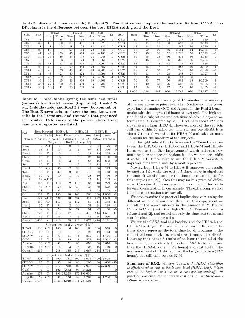
We now turn to the constrained synthetic models seen inTable 5. In this table the column labelled ‘Best’ representsthe best known results for CASA (the only tool on whichthese synthetic benchmarks have been reported to date). Forthe constrained problems HHSA performs as well or betterthan the best known results (except in one case) despitethe fact that CASA is optimized for these subjects. HHSArequires 39 fewer rows overall than the best reported results.
The last comparison we make is with the Real bench-marks. Table 6 shows a comparison for all of our real sub-jects against a set of existing tools which were reported inthe literature (references provided in the table). Again wesee that the HHSA algorithm performs as well or better thanall of the other tools. For the IBM benchmarks HHSA re-duces the overall number of rows in our samples by 52, andfor the open source applications HHSA reduces the 2-wayby 3 rows, and the 3-way by 54 rows.Summary of RQ1. We conclude that the quality of resultsobtained by using HHSA is high. While we do not producethe best results on every model, we are quite competitive andfor all of the real subjects we are as good as, or improve uponthe best known results.
5.2 RQ2: Efficiency of Hyperheuristic HHSATable 7 summarizes the average execution time in seconds
per subject within each group of benchmarks, using the threeconfigurations of HHSA. The average execution time for theexperiments with low configuration is about 1000 seconds(or 17 minutes).
7
Table 5: Sizes and times (seconds) for Syn-C2. The Best column reports the best results from CASA. TheDf column is the di↵erence between the best HHSA setting and the Best.
Sub. BestHHSA-L HHSA-M HHSA-H
Df Sub. BestHHSA-L HHSA-M HHSA-H
DfSize Time Size Time Size Time Size Time Size Time Size Time
Table 6: Three tables giving the sizes and times(seconds) for Real-1 2-way (top table), Real-2 2-way (middle table) and Real-2 3-way (bottom table).The Best Known column shows the best known re-sults in the literature, and the tools that producedthe results. References to the papers where theseresults are reported are listed.
Despite the overall average of 17 minutes, the majorityof the executions require fewer than 5 minutes. The 3-wayexperiments running GCC and Apache in the Real-2 bench-marks take the longest (1.6 hours on average). The high set-ting for this subject set was not finished after 3 days so weterminated it (indicated by ’-’). HHSA-M is about 12 timesslower overall than HHSA-L. However, most of the subjectsstill run within 10 minutes. The runtime for HHSA-H isabout 7 times slower than for HHSA-M and takes at most1.5 hours for the majority of the subjects.
On the right side of this table we see the ‘Time Ratio’ be-tween the HHSA-L vs. HHSA-M and HHSA-M and HHSA-H, as well as the ‘Size Improvement’ which indicates howmuch smaller the second variant is. As we can see, whileit costs us 12 times more to run the HHSA-M variant, itimproves our sample sizes by almost 3 percent.
Moving from HHSA-M to HHSA-H improves our resultsby another 1%, while the cost is 7 times more in algorithmruntime. If we also consider the time to run test suites forthis sample (see [19]), then this may make a practical di↵er-ence. Consider if it takes overnight to run a full test suitefor each configuration in our sample. The extra computationtime for construction may pay o↵.
We next examine the practical implications of running thedi↵erent variants of our algorithm. For this experiment werun all of the 2-way subjects in the Amazon EC2 (ElasticCompute Cloud) with the High-CPU On-Demand Instance(c1.medium) [2], and record not only the time, but the actualcost for obtaining our results.
We run the CASA tool as a baseline and the HHSA-L andHHSA-M settings. The results are shown in Table 8. Thetimes shown represent the total time for all programs in therespective benchmarks (averaged over 5 runs). The HHSA-L setting took about 8 tenths of an hour to run all of thebenchmarks, but cost only 13 cents. CASA took more timethan the HHSA-L variant (2.9 hours) and cost $0.49. Themedium variant of HHSA required the longest runtime (12.7hours), but still only cost us $2.09.
Summary of RQ2. We conclude that the HHSA algorithmis e�cient when run at the lowest level (HHSA-low). Whenrun at the higher levels we see a cost-quality tradeo↵. Inpractice, however, the monetary cost of running these algo-rithms is very small.
8
Table 7: Running times (seconds) of the di↵erent levels of HHSA. Each time represents the average timefor each individual model within the benchmark. Time Ratio and Size Impr. show the ratio and percent(respectively) between the L/M and M/H settings. ’-’ indicates that no result was obtained after 3 days.
Subject Sets HHSA-L Time HHSA-M Time HHSA-H TimeHHSA-L vs. HHSA-M HHSA-M vs. HHSA-H
Table 8: Sizes and times (seconds) and dollar cost for running each of the benchmark sets to completion inthe Amazon EC2 Cloud with the High-CPU On-Demand Instance (c1.medium) [2].
SubjectsCASA HHSA-L HHSA-M
Time (s) Cost$ Size Time (s) Cost $ Size Time (s) Cost$ SizeSyn-S2 5,777 0.26 808 220 0.01 820 2,350 0.11 805Real-2 119 0.01 1,451 185 0.01 1,421 4,660 0.21 1,417Real-1 265 0.01 233 383 0.02 222 3,971 0.18 216Syn-C2 4,440 0.20 1,053 2,029 0.09 1,067 34,736 1.59 1,005
We now examine how e�cient and e↵ective each of thesearch navigation operators are in isolation. To answer thisquestion, we built seven versions of the simulated anneal-ing algorithm, all using the HHSA-L settings. Each of thefirst six versions contains a single operator. For the seventhversion, HH-Random, we include all operators, but the op-erator to use at each stage is chosen at random (with nointelligence).
The overall results for operator comparison are shown inTable 9. Each of the operators is listed in a row (Op1-Op6). The numbers correspond to their earlier descriptions(see Section 3.3). The next row is HH-Random, followed bythe HHSA-L variant. The best operators on their own ap-pear to be the “mutation” operators. Operator 4 (multiplemutation) seems to work relatively well on its own as doesOperator 1 (single mutation). The HH-Rand variant per-forms second best which indicates that the combination ofoperators is helping the search, and it runs relatively fast,however without the guidance from learning it appears notdo quite as well as the HHSA-L algorithm.
Summary of RQ3. We conclude that there is a di↵er-ence between e↵ectiveness of each of the operators and thatcombining them contributes to a better quality solution.
Table 9: “Navigation operator” comparison. Op1to Op6 uses the standard SA with and individualsearch operator. HH-Rand makes a random choiceat each evaluation. All variants are run using thelow configuration. Time is in seconds.
To determine if the operators that are selected by thehyperheuristic SA algorithm are learned we examine Table10 and Figure 2. We first look at the graphs. The x-axis
represents the di↵erent problem states which is the numberof missing tuples that the problem has left to cover. Onthe left part of the graph, there are many tuples remaininguncovered, and towards the right, very few. We plot thereward scores from our learning algorithm for each operatorat each stage (a higher reward score means the operatoris more likely to be selected). We show this data for onesynthetic and one real subject (due to space limitations), S2-8 (top), and TCAS (bottom). As we can see, early on whenthe problem is easier, most of the operators are close to thesame reward value with one or two standing out (Operator 4in S2-8 and Operator 5 in TCAS). This changes as we havefewer tuples to cover; most of the operators move towards anegative reward with a few remaining the most useful. Notonly do we see di↵erent “stages” of operator selection, butwe also see two di↵erent patterns.
We examine this further by breaking down data from eachbenchmark set into stages. We evenly split our data byiteration into an early (S1), middle (S2) and late (S3) stageof the search. For each, we select the pairs of operatorsthat are selected most often across each benchmark set. Forinstance, Op1+Op4 is selected most often at stage S1 for 6subjects in the set Syn-2 (see Table 10). In stage 1 we seethat Op4+Op5 is selected most often overall, while in stage 2it is Op1+Op4 and in stage 3 it is Op1+Op6. Within eachbenchmark we see di↵erent patterns. For instance, in thefirst stage Op1+Op5 is selected most often by the Syn-C2(constrained synthetic) which is di↵erent from the others. Instage 2 again we see that the Syn-C2 has a di↵erent patternof operator selection with Op1+Op4 being selected 14 times.In other sets such as the Real 1 we see that the Op4+Op6combination is chosen most often.
Summary of RQ4. We see evidence that the Hyperheuris-tic algorithm is learning both at di↵erent stages of searchand across di↵erent types of subjects.
9
-25
-20
-15
-10
-5
0
5
10
15
85 77 66 55 42 31 28 22 18 12 8 3 1
Rewa
rd S
core
s
Missing Tuples
Op1 Op2 Op3 Op4 Op5 Op6
-8
-6
-4
-2
0
2
4
6
51 44 37 31 26 21 15 9 4 1
Rewa
rd S
core
s
Missing Tuples
Op1 Op2 Op3 Op4 Op5 Op6
Figure 2: Subject: S2-8 (top) and TCAS (bottom).X-axis shows number of tuples left to cover. Y-axisshows the learning algorithm’s reward scores.
6. RELATED WORKResearch on the generation of covering arrays has a long
history [13,30]. Many of the original tools were developed towork on unconstrained problems (or require manual remod-eling) [8, 12, 27, 31], while more recent ones are specializedfor constrained problems [4,19,36], or higher strengths [26].
Another classification is the type of algorithm used. Ingeneral the greedy approaches such as AETG, IPO andPICT are fastest, but may create larger sized samples [8,15, 27] while heuristic search produces smaller array sizes,but requires longer running times [12,19,28,31].
Garvin et al. [19] present a break-even approach to quan-tify the true cost between algorithms, which considers thetime it costs to test the software as well as the time to buildthe arrays (i.e. this includes the impact of sample size aswell as the generation time), and conclude that size tends tobe the limiting factor for systems with even a short testingtime per element in the covering array.
The mathematics community has developed both mathe-matical (constructive) and probabilistic proofs of bounds fora wide range of problems (see [14]), but these are syntheticmodels which may or may not be consistent with practice.We compare against some of these in this paper.
Another trend in CIT has been to specialize the construc-tion for a particular process (incremental or adaptive) [17,18]which either builds covering arrays in stages to map to a par-ticular test process, or iteratively modifies the model as ituncovers unknown constraints. But these techniques use astandard CIT algorithm as a primitive core, and are there-fore orthogonal to our work.
Finally there are algorithms that are devised to work onvery large models (such as the complete Linux kernel with6,000+ factors) [32]. Our use of tunable settings for HHSAis consistent with this potential need.
Given the large mix of approaches to date, Calvagna et al.built CITLAB [6], a tool and language that brings togethermany other di↵erent tools for CIT into a single interface andframework. This allows the tester to execute di↵erent toolson the same benchmarks where the goal is to determine the“best” choice.
Table 10: Learning Strategies. Three stages ofthe algorithm (S1-early), (S2-middle) and (S3-late)showing the pairs of operators chosen the most oftenby stage and subject set.
However, this framework does not remove the limitationthat we are trying to solve – the tester still has to decidewhich algorithm works on which problem. Our approachdi↵ers from these approaches because our aim is not to bethe “best” for any particular problem type, but to providea generalist tool armed with online learning, that automat-ically adapts to each di↵erent problem model it encounters.
7. CONCLUSIONSIn this paper we have presented a hyperheuristic algorithm
for constructing CIT samples. We have shown that the al-gorithm is general and learns as the problem set changesthrough a large empirical study on a broad set of bench-marks. We have shown that the algorithm is e↵ective whenwe compare it across the benchmarks and other algorithmsand results from the literature.
We have also seen that the use of di↵erent tunings for thealgorithm (low, medium and high) will provide a quality-costtradeo↵ with the higher setting producing better results, buttaking longer to run. When we examine the practicality ofsuch an algorithm, we see that the monetary cost for run-ning the algorithm is quite small when using today’s cloud($2.09).
Finally, we have examined the various stages of learning ofour algorithm and see that the di↵erent heuristic operatorsare more e↵ective at di↵erent stages (early, middle, late)and that they vary across programs and benchmarks. It isthis ability to learn and adapt that we believe is the mostimportant aspect of this search.
As future work we will look at alternative tunings for thealgorithm so that we can scale to very large problems (a verylow setting) and can find even smaller sample sizes (a veryhigh setting). We will also incorporate new operators andwill look at alternative algorithms for the outer layer, suchas genetic algorithms.
10
8. REFERENCES[1] S. Ali, L. C. Briand, H. Hemmati, and R. K.
Panesar-Walawege. A systematic review of theapplication and empirical investigation of search-basedtest-case generation. IEEE Transactions on SoftwareEngineering, pages 742–762, 2010.
[2] Amazon. EC2 (Elastic Compute Cloud). Available athttp://aws.amazon.com/ec2/.
[3] E. K. Burke, M. Gendreau, M. Hyde, G. Kendall,G. Ochoa, E. Ozcan, and R. Qu. Hyper-heuristics: asurvey of the state of the art. Journal of theOperational Research Society, 2013. to appear.
[4] A. Calvagna and A. Gargantini. A formal logicapproach to constrained combinatorial testing. Journalof Automated Reasoning, 45:331–358, December 2010.
[5] A. Calvagna and A. Gargantini. T-wise combinatorialinteraction test suites construction based on coverageinheritance. Software Testing, Verification andReliability, 22(7):507–526, 2012.
[6] A. Calvagna, A. Gargantini, and P. Vavassori.Combinatorial interaction testing with CITLAB. InICST, pages 376–382, 2013.
[7] M. Chateauneuf and D. L. Kreher. On the state ofstrength-three covering arrays. Journal ofCombinatorial Designs, 10(4):217–238, 2002.
[8] D. M. Cohen, S. R. Dalal, M. L. Fredman, and G. C.Patton. The AETG system: an approach to testingbased on combinatorial design. IEEE Transactions onSoftware Engineering, 23(7):437–444, 1997.
[9] M. Cohen, M. Dwyer, and J. Shi. Constructinginteraction test suites for highly-configurable systemsin the presence of constraints: A greedy approach.Software Engineering, IEEE Transactions on,34(5):633–650, 2008.
[10] M. B. Cohen, C. J. Colbourn, and A. C. H. Ling.Augmenting simulated annealing to build interactiontest suites. In Proceedings of the 14th InternationalSymposium on Software Reliability Engineering,ISSRE ’03, pages 394–, Washington, DC, USA, 2003.IEEE Computer Society.
[11] M. B. Cohen, M. B. Dwyer, and J. Shi. Interactiontesting of highly-configurable systems in the presenceof constraints. In Proceedings of the 2007 internationalsymposium on Software testing and analysis, ISSTA’07, pages 129–139, New York, NY, USA, 2007. ACM.
[12] M. B. Cohen, P. B. Gibbons, W. B. Mugridge, andC. J. Colbourn. Constructing test suites forinteraction testing. In Proceedings of the 25thInternational Conference on Software Engineering,ICSE ’03, pages 38–48, Washington, DC, USA, 2003.IEEE Computer Society.
[13] C. J. Colbourn. Combinatorial aspects of coveringarrays. Le Matematiche (Catania), 58:121–167, 2004.
[14] C. J. Colbourn. Covering array tables. Available athttp://www.public.asu.edu/⇠ccolbou/src/tabby/catable.html, 2012.
[15] J. Czerwonka. Pairwise testing in real world. InPacific Northwest Software Quality Conference, pages419–430, October 2006.
[16] H. Do, S. G. Elbaum, and G. Rothermel. Supportingcontrolled experimentation with testing techniques:An infrastructure and its potential impact. Empirical
Software Engineering: An International Journal,10(4):405–435, 2005.
[17] E. Dumlu, C. Yilmaz, M. B. Cohen, and A. Porter.Feedback driven adaptive combinatorial testing. InProceedings of the 2011 International Symposium onSoftware Testing and Analysis, pages 243–253, 2011.
[18] S. Fouche, M. B. Cohen, and A. Porter. Incrementalcovering array failure characterization in largeconfiguration spaces. In International Symposium onSoftware Testing and Analysis (ISSTA), pages177–187, July 2009.
[19] B. Garvin, M. Cohen, and M. Dwyer. Evaluatingimprovements to a meta-heuristic search forconstrained interaction testing. Empirical SoftwareEngineering, 16(1):61–102, 2011.
[20] B. J. Garvin, M. B. Cohen, and M. B. Dwyer. Animproved meta-heuristic search for constrainedinteraction testing. In Proceedings of the 2009 1stInternational Symposium on Search Based SoftwareEngineering, SSBSE ’09, pages 13–22, Washington,DC, USA, 2009. IEEE Computer Society.
[21] M. Harman. The current state and future of searchbased software engineering. In 2007 Future of SoftwareEngineering, FOSE ’07, pages 342–357, Washington,DC, USA, 2007. IEEE Computer Society.
[22] M. Harman, E. Burke, J. Clark, and X. Yao. Dynamicadaptive search based software engineering. InProceedings of the ACM-IEEE internationalsymposium on Empirical software engineering andmeasurement, ESEM ’12, pages 1–8, 2012.
[23] M. Harman, A. Mansouri, and Y. Zhang. Search basedsoftware engineering: Trends, techniques andapplications. ACM Computing Surveys, 45(1):Article11, November 2012.
[24] B. Hnich, S. Prestwich, E. Selensky, and B. Smith.Constraint models for the covering test problem.Constraints, 11:199–219, 2006.
[25] C. Le Goues, M. Dewey-Vogt, S. Forrest, andW. Weimer. A systematic study of automatedprogram repair: Fixing 55 out of 105 bugs for $8 each.In ICSE, pages 3–13, 2012.
[26] Y. Lei, R. Kacker, D. R. Kuhn, V. Okun, andJ. Lawrence. Ipog-ipog-d: e�cient test generation formulti-way combinatorial testing. Software TestingVerification and Reliability, 18:125–148, September2008.
[27] Y. Lei and K. Tai. In-parameter-order: a testgeneration strategy for pairwise testing. InHigh-Assurance Systems Engineering Symposium,1998. Proceedings. Third IEEE International, pages254–261, 1998.
[28] J. Martinez-Pena, J. Torres-Jimenez,N. Rangel-Valdez, and H. Avila-George. A heuristicapproach for constructing ternary covering arraysusing trinomial coe�cients. In Proceedings of the 12thIbero-American conference on Advances in artificialintelligence, IBERAMIA’10, pages 572–581, 2010.
[29] P. Nayeri. Post-Optimization: Necessity Analysis forCombinatorial Arrays. Ph.D. thesis, Department ofComputer Science and Engineering, Arizona StateUniversity, April 2011.
[30] C. Nie and H. Leung. A survey of combinatorial
[31] K. Nurmela. Upper bounds for covering arrays bytabu search. Discrete Applied Mathematics,138(1-2):143–152, 2004.
[32] G. Perrouin, S. Sen, J. Klein, B. Baudry, and Y. l.Traon. Automated and scalable t-wise test casegeneration strategies for software product lines. InProceedings of the 2010 Third InternationalConference on Software Testing, Verification andValidation, pages 459–468, 2010.
[33] J. Petke, S. Yoo, M. B. Cohen, and M. Harman.E�ciency and early fault detection with lower andhigher strength combinatorial interaction testing. InProceedings of the 9th Joint Meeting of the EuropeanSoftware Engineering Conference and the ACMSIGSOFT Symposium on the Foundations of SoftwareEngineering (ESEC/FSE’13), pages 26–36, August2013.
[34] O. Raiha. A survey on search based software design.Technical Report Technical Report D-2009-1,
Department of Computer Sciences, University ofTampere, 2009.
[35] D. Richard Kuhn and V. Okum. Pseudo-exhaustivetesting for software. In Proceedings of the 30th AnnualIEEE/NASA Software Engineering Workshop, SEW’06, pages 153–158, Washington, DC, USA, 2006.IEEE Computer Society.
[36] I. Segall, R. Tzoref-Brill, and E. Farchi. Using binarydecision diagrams for combinatorial test design. InProceedings of the 2011 International Symposium onSoftware Testing and Analysis, ISSTA ’11, pages254–264, New York, NY, USA, 2011. ACM.
[37] J. Stardom. Metaheuristics and the Search forCovering and Packing Arrays. Thesis (M.Sc.)–SimonFraser University, 2001.
[38] R. S. Sutton and A. G. Barto. ReinforcementLearning: An Introduction. MIT Press, 1998.
[39] Y.-W. Tung and W. Aldiwan. Automating test casegeneration for the new generation mission softwaresystem. In Aerospace Conference Proceedings, 2000IEEE, volume 1, pages 431–437 vol.1, 2000.