1 Abstract A Dynamic Analysis of Mergers Gautam Gowrisankaran 1995 The dissertation examines the dynamics of firm behavior using computational methods, with the goal of modeling mergers more realistically than previous studies in order to examine policy implications. In this model, mergers, investment, entry and exit are endogenous choice variables rationally chosen by firms in the industry in order to maximize expected future profits. The model differs from previous studies in two ways: first, it directly specifies a process through which firms can merge and predicts which mergers will occur at different states; second, it incorporates dynamic determinants of firm behavior (namely entry, exit and investment). In Chapter 1, I discuss criteria for designing an endogenous merger process and I detail the processes chosen and corresponding results. The results show that by not incorporating the effects of investment and entry on the merger behavior of firms, the static literature is overpredicting the probability of mergers; this type of result has not been shown before since it can only be shown with an endogenous model. In Chapter 2, I examine antitrust policy implications using the dynamic model of endogenous mergers and compare these to the planner and colluder solutions. The results show first that a wide range of intermediate antitrust policies leads to a
Transcript
1
Abstract
A Dynamic Analysis of Mergers
Gautam Gowrisankaran
1995
The dissertation examines the dynamics of firm behavior using computational
methods, with the goal of modeling mergers more realistically than previous studies
in order to examine policy implications. In this model, mergers, investment, entry
and exit are endogenous choice variables rationally chosen by firms in the industry
in order to maximize expected future profits. The model differs from previous studies
in two ways: first, it directly specifies a process through which firms can merge and
predicts which mergers will occur at different states; second, it incorporates dynamic
determinants of firm behavior (namely entry, exit and investment). In Chapter 1, I
discuss criteria for designing an endogenous merger process and I detail the
processes chosen and corresponding results. The results show that by not
incorporating the effects of investment and entry on the merger behavior of firms,
the static literature is overpredicting the probability of mergers; this type of result
has not been shown before since it can only be shown with an endogenous model. In
Chapter 2, I examine antitrust policy implications using the dynamic model of
endogenous mergers and compare these to the planner and colluder solutions. The
results show first that a wide range of intermediate antitrust policies leads to a
2
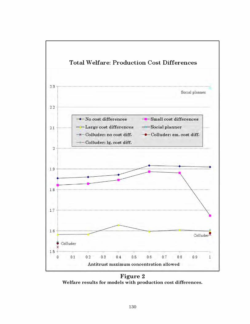
higher total welfare than either a complete merger prohibition or no antitrust law.
In addition, they show that with production cost differences, merger synergies and
barriers to entry, the implications of different antitrust policies are surprising and
very different than those predicted by static non-endogenous merger models.
Finally, the model uses its rational framework to explain the puzzle, discussed in
the empirical literature, of why acquired firms seem to capture all of the gains from
mergers. In Chapter 3, I discuss the issues surrounding the design and computation
of the model. In particular, I examine when equilibria to the merger processes are
likely to exist, the choice of specifications necessary to allow for computation, and
the computational details of the processes. This discussion is of interest in order to
further develop computational merger models and to design computational models of
other oligopolistic games.
3
A Dynamic Analysis of Mergers
A Dissertation Presented to the Faculty of the Graduate School
of Yale University
in Candidacy for the Degree of Doctor of Philosophy
Table of Contents: Abstract............................................................................................................................ 1 Title Page ......................................................................................................................... 3 Table of Contents............................................................................................................. 5 Introduction ..................................................................................................................... 6 Chapter 1: A Dynamic Model of Endogenous Horizontal Mergers.......................................... 12 Section 1: Introduction ...................................................................................... 13 Section 2: The Industry and Merger Model...................................................... 18 Section 3: Results............................................................................................... 36 Section 4: Conclusions and Further Research ................................................. 50 References .......................................................................................................... 54 Figures................................................................................................................ 56 Tables ................................................................................................................. 58 Chapter 2: Policy Implications of a Dynamic Horizontal Merger Model ................................ 63 Section 1: Introduction ...................................................................................... 64 Section 2: The Model and Antitrust Results .................................................... 70 Section 3: Differences in Production Costs....................................................... 86 Section 4: Other Cost Differences ..................................................................... 94 Section 5: Stock Market Values ...................................................................... 103 Section 6: Conclusions ..................................................................................... 110 References ........................................................................................................ 114 Tables ............................................................................................................... 117 Figures.............................................................................................................. 129 Chapter 3: Computing Endogenous Merger Models .............................................................. 133 Section 1: Introduction .................................................................................... 134 Section 2: Modeling Endogenous Merger Processes ...................................... 136 Section 3: Solving Endogenous Merger Games.............................................. 167 Section 4: Solving the Dynamic Equilibrium ................................................. 183 Section 5: Conclusions ..................................................................................... 201 References ........................................................................................................ 203
6
Introduction:1 The purpose of this dissertation is to analyze the effects of mergers between
competitors in an industry. The main goal of the analysis is to predict which mergers
occur and what the consequences of the mergers that do occur are, in order to derive
more realistic results than have been obtained by previous models. Mergers are of
interest to economists and policy-makers due to their frequency and their potential
effects on the economic performance of industries. Because of their importance,
mergers have been studied by many authors with many different goals. Over the
past century, different schools have studied the collusive effects of mergers, the
empirical efficiency gains from mergers, and the potential of antitrust law to
encourage inefficient industry structures. Notable among these schools of study is
the Chicago School. One of the main contributions of the Chicago School was to
caution that strict antitrust policy might have deleterious dynamic effects;; however,
the proponents of the Chicago School did not attempt to model the merger process
mathematically. Most recent advances in studying mergers have used game theory,
in order to be able to mathematically predict which mergers are profitable. Thus,
typical recent studies have attempted to find which mergers yield a static gain to
1 I would like to thank my advisors Steve Berry and Ariel Pakes, and also Dan Ackerberg, Kathie Barnes, David Pearce, Ben Polak, Matthew Ryan, Bob Town, Paul Willen, Lin Zhou, and seminar participants at Boston University, Northwestern University, U.S. Department of Justice, University of Minnesota and Yale University for helpful comments. I would also like to thank the Social Sciences and Humanities Research Council of Canada (Doctoral Fellowship 752-93-0054), the Alfred P. Sloan Foundation (Doctoral Dissertation Fellowship), Fonds pour la formation de chercheurs et l’aide à la recherche du Québec (Bourse de maitrise) and Yale University (University Fellowship, Overbrook Fellowship and Enders Fellowship) for financial support during my doctoral studies.
7
producers and which mergers are socially optimal in a variety of settings, including:
a Cournot model, a Bertrand model, a Cournot model with cost differences, a
Hotelling model, a model where merging firms are perfect complements, and a model
where there are synergies between merging firms. While the game theory models
have examined different issues, they have mostly used the same paradigm: that
there is a merger process, followed by some one-shot production game that is played
by the firms that remain after the merger process is completed. Thus, the game
theory literature is not able to incorporate the important effects that dynamic
determinants, such as investment, entry and exit, will have on the outcome of the
merger process. In addition to the game theory literature on mergers, there is a
related literature, on endogenous coalition formation, that has attempted to explore
which coalitions are likely to result from a given set of agents with defined payoffs.
As coalitions that cannot be broken are mathematically identical to mergers, this
literature is also relevant to any study of mergers. However, the endogenous merger
literature has thus far used very simple conceptions of firms and has not been able
to yield predictions for which coalitions will form except in some restrictive cases.
While mergers have been studied a great deal by previous works, none of the
papers in the literature has examined mergers in a setting where firms can choose
merger decisions according to some well-specified process, which provides the
modeler with the ability to examine which mergers firms choose. Alternately put,
none of the papers in the literature has endogenized the merger process. Because
none of the papers in the literature has examined mergers in a fully endogenous,
dynamic setting, none of the papers has been able to analyze the central questions of
which mergers will occur, and what the welfare and other effects of the mergers that
8
do occur will be. The primary contribution of this dissertation is that it is the first
model which predicts the patterns and occurrences of mergers in industries, and
then uses these predictions in order to develop antitrust policy implications for a
variety of industry phenomena. The model predicts the patterns and occurrences of
mergers using a well-defined model where firms rationally choose merger decisions,
as well as entry, exit and investment decisions in order to maximize the expected
discounted value of their net future profits, conditional on their information. In
addition to this primary contribution, the other contribution of this dissertation is in
furthering the theories of coalition formation, auctions with externalities and the
general computational modeling of oligopolistic industry structures.
As I discussed above, the model that I present in this dissertation is able to
explain mergers in ways that no other model has attempted. The primary reason
why the model is able to endogenize the merger process is that, while others have
attempted to derive analytical solutions to their merger models, I am using
computational methods. The basic methodology that I use is to choose parameter
values, compute the equilibrium for the parameter values and then explore the
welfare and industry implications that result from the given parameter values. In
order to examine the effects of different policies and different types of industries, I
change the parameters to reflect different industries and examine how this changes
the results of the model. In order to determine the sensitivity of the model to
different specifications, I change the specifications and repeat the process. With a
computational model such as this one, I am able to examine a more complex vision of
an industry than analytical models. Thus, I am able to have an endogenous merger
process, incorporate dynamic determinants of firm behavior and evaluate how the
9
industry performance changes for different policies and institutions, all due to the
computational nature of my model.
Because I am answering central questions of the merger debate that have not
been answered before, the discussion in this dissertation has many interesting
facets. The discussion explores what criteria one needs to examine in designing a
dynamic, endogenous model of mergers and examines the generality of the model
presented by evaluating the results. In addition, the model is able to determine the
size and direction of the bias that static models will have by not incorporating
dynamics in their models. With the model, I examine the implications of antitrust
policies and explore optimal policies and first-best solutions. I also examine how
optimal antitrust policies change when such factors as barriers to entry or
production cost differences are present in the industry. Finally, I use the model to
reexamine the empirical paradox of why firms choose to make acquisitions when the
gains from mergers appear to accrue exclusively to the acquired firm. In addition to
the results of the model, I discuss the theoretical basis for the endogenous merger
mechanisms used and the techniques used in computing the merger and overall
dynamic processes for the model.
While the discussion of the model as presented in the dissertation is self-
contained, the model developed here is of use in future research. In particular, as
the parameters of the model can be changed to examine different industries, the
model can serve as a basis for structural empirical work. In the future, economists
can estimate relevant structural parameters for industries of interest, and use
variants of this model to examine the implications of different antitrust policies for
these industries. Although this is a difficult task, it will allow economists to
10
incorporate the effects of dynamics and consistently estimate the effects of
government antitrust policies on the future performance of industries. While this
task has not been accomplished before, it is important to policy-makers in
determining which policies to enact. More generally, one can use the model with
stylized versions of industries in order to examine the size and direction of the bias
that is introduced into the results by examining the effects of mergers in a static
setting and by not endogenizing the merger process. Thus, applications of the
merger model to sectors that are the subject of antitrust interest, such as the
hospital industry, the cement industry and the timber industry, are likely to be
feasible in the near future.
In spite of the wide range of issues that I discuss in this dissertation, there
are limitations to the issues that I can examine and the generality of the results. In
particular, because of the computational nature of the model, the results of the
model depend on the parameters in ways that cannot be determined fully. The best
technique that can be used to determine the generality of the results is to vary the
parameters and compare the results of the model with different parameters.
However, the ability to do this is limited by the computational complexity of the
model, which is substantial. In addition, because I am specifying processes by which
firms merge, invest, exit and enter, each process is structural and hence the choice
of structure is arbitrary. Finally, because of the nature of the model, given a set of
arbitrary parameter values, one cannot be assured that the equilibrium that the
algorithm converges to is unique, that the algorithm will even converge to an
equilibrium, or that there even exists an equilibrium. Thus, the results presented
here should not be thought of as the last word on modeling mergers endogenously,
11
but rather the first word. While I am able to obtain many interesting and surprising
results with this model, and while this is the first model to predict the occurrence of
mergers, there is room to make the endogenous merger process and other processes
more general and to make the model less cumbersome.
The remainder of this dissertation is divided as follows. Chapter 1 discusses
the choice of model and examines the specification of the model and the necessity of
incorporating dynamics in the model. Chapter 2 discusses many different antitrust
policy implications of the model and examines the paradox of the splitting of gains
from mergers. Finally, Chapter 3 provides a discussion of the computational issues
of the merger model, including an examination of the computation of auctions with
externalities.
12
Chapter 1:
A Dynamic Model of Endogenous Horizontal Mergers.
13
Section 1: Introduction
Economists have long been interested in studying horizontal mergers,
because of the important effects that they have, and because they occur in vast
numbers. As mergers are of concern to policymakers only in industries with a
limited number of firms, recent advances have analyzed mergers using game theory.
The first major paper that analyzes mergers with a game theoretic approach is
Salant-Switzer-Reynolds (1983 - hereafter S-S-R), which shows that with Cournot
interactions between firms that produce a homogeneous product, mergers for
oligopoly will generally not be profitable in a static game, unless the original number
of firms is small, and a very large proportion of existing firms actually merge.1 Other
papers in the literature have obtained results for a differentiated products Bertrand
setting (see Deneckere and Davidson (1985)), with cost differences (see Perry and
Porter (1985)), and when there are synergies between firms (see Farrell and Shapiro
(1990)). These papers have all used models that are static in nature and accordingly
have not incorporated the effects that dynamic determinants of firm behavior, such
as entry, exit and investment, have on the results of the merger process. There are
several important economic reasons why entry, exit and investment will have large
effects on which mergers occur in an industry, and what the welfare consequences of
such mergers will be. For example, although one may think that mergers lower
consumer welfare by increasing concentration, entry into the industry may increase
if mergers are allowed, and counterbalance the increase in concentration. Or,
mergers may allow firms to partially internalize the negative externality from their
1 The proportion must approach one as the number of firms approaches infinity for any mergers to take place.
14
investment, and thus increase profits. Because these dynamic behaviors are
important economic determinants of mergers, some papers, such as Berry and Pakes
(1993) and Cheong and Judd (1993), have analyzed mergers with dynamic game
theoretic industry models.
While economists have learned a great deal from the static and dynamic
game theoretic merger literature, none of the above papers has provided a
framework which predicts which mergers are likely to arise in a given industry.
Their approach has largely been, instead, to examine the consequences of particular
mergers, and to see whether these particular mergers are profitable, relative to no
merger. As a result, one cannot fully understand the importance that dynamics have
to the consequences of firm merger behavior. For instance, if entry is possible, firms
that would have otherwise chosen to merge may not merge, as they know that future
entry would make any profits from the increased concentration transitory. Or, a
weak firm may choose not to exit an industry, knowing that if it were to remain, it
would be acquired by a large competitor sooner or later. Finally, a firm may choose
not to acquire another firm in the current period even if such a merger is profitable
relative to no merger, knowing that in the future it will be in a better bargaining
position and be able to acquire the firm for a lesser price. These examples show that
one cannot fully evaluate the effects of dynamics on mergers without endogenizing
the merger process and examining how the mergers actually chosen by firms change
when dynamics enter into their decisions.
In addition to determining whether or not a dynamic model is necessary to
analyze merger behavior, there are many other reasons why economists would like
to be able to evaluate which mergers will take place in an industry. In order to
15
investigate the welfare effects of antitrust or other government policies one must use
a model that predicts how policies affect future entry, exit, investment and mergers,
and through that the future structures and performance of the industry, as
otherwise one cannot evaluate optimal long-run policies. Indeed, any analysis of
mergers that does not endogenize the merger process will not be able to predict
future actions that result from current policies and hence cannot predict the future
welfare and industry effects of current policies.
This paper presents a model of endogenous horizontal mergers in a stylized
industry. In the model, firms choose their merger decisions via a simple bidding
process or via an auction process. Thus, conditional on parameters, the model is able
to predict the equilibrium probability that any firm will choose to merge with any
other firm given an industry structure. Because of the potential importance of entry,
exit and investment in determining the effects of mergers, the model incorporates
dynamics: in addition to choosing merger decisions, existing firms and potential
entrants choose entry, exit, and investment decisions in order to compete in an
infinitely-lived industry. The primary goal of the model is to serve as a tool for
analyzing the effects of different policies. It can accomplish this goal in ways that
other models have not been able to because it is endogenizing the merger process
and using a dynamic framework. There are several ways in which I have used and
am planning to use the model to accomplish its goal. First, in this chapter, I use the
model in order to find how large a role entry, exit and investment play in
determining the effects of mergers, and I examine to what extent the conclusions of
the model are dependent on specifications. In Chapter 2, I use the model in order to
analyze the effects of antitrust policy in stylized industries and examine how the
16
optimal antitrust policies change when such factors as barriers to entry and
increasing returns are present. Finally, as the ultimate goal of this model is to
understand actual industries more precisely, this model serves as a tool for future
empirical work. Empirical studies can estimate the underlying parameters of the
model for specific industries, and then use the model to evaluate the effects of
antitrust and other policies for actual industries.
The dynamic framework of firm behavior that I use in this model is based on
the framework developed by Ericson and Pakes (1995), and modifies this framework
to allow for endogenous mergers. Accordingly, the conception is of an infinitely-lived
industry modeled in discrete time, where current firms merge, invest, exit and
produce, potential entrants enter, and all agents rationally make their choices in
order to maximize their expected discounted value (EDV) of future profits. For the
results presented in this chapter, firms invest in order to increase their capacity
levels in future periods (following Berry and Pakes) and statically are Cournot
competitors in a homogeneous goods market. While this structure was chosen in
order for the stylized results to be simple, it is possible to use the endogenous
merger model with different static and dynamic interactions between firms and
hence to use this model to examine the implications of mergers in different
industries.
Because I am endogenizing the merger, investment, entry and exit processes
and modeling dynamics explicitly, the model is elaborate and non-linear. Thus, it is
not possible to analytically solve for an equilibrium of the model. Instead, the
technique that I use is to pick particular parameter values, compute equilibria
numerically for these parameter values, and then simulate the industry dynamics,
17
in order to be able to uncover the distribution of the industry particulars (i.e.
investment levels, sizes of firms, lifespans, amount of entry, etc.) that occur in the
equilibrium distribution of the industry. While the goal of this chapter is to
theoretically analyze the effects of incorporating dynamics in a merger model, as the
theory that I am interested in is too complex to obtain analytical results, I instead
find numerical answers. Thus, the answers to the theoretical questions are largely
in the form of results from computational calculations and simulations of the model,
rather than from theorems. In Chapter 2, I attempt to answer policy-relevant
questions concerning mergers using these same computational methods and this
model as a basis.
With this stylized model, I have computed equilibria and simulated the
industry using equilibrium policies in order to uncover the characteristics of the
industry, in terms of welfare and policy variables. In order to test the sensitivity of
the model to parameter changes, I have computed the models for different
parameters and specifications, and illustrated how these specifications change the
results of the model. The specifications I have examined include modeling mergers
with different coalition formation processes, comparing them to an industry where
no mergers are allowed, and to an industry where firms’ decisions to merge are
based only on current period profits, similarly to the static literature on mergers.
The results show, primarily, that is possible to develop a model of endogenous
mergers that is computable, incorporates dynamic determinants of firm behavior,
and yields reasonable results. In particular, the ordering of the firms in the merger
process does not have major effects on the industry dynamics, which demonstrates
18
that the model is not overly sensitive to changes in specification, and changes in the
size of the synergy distribution have the effects that one would expect. While the
results are different depending on whether a take-it-or-leave-it or auction process is
used in making merger decisions, the reason for the difference is easily explained by
the nature of the different processes. In addition, the results show that incorporating
dynamics into a merger model may lead to important improvements in the
predictive power of the model. This is apparent largely for two reasons: first, the
level of the principal dynamic components of the model (namely entry, exit and
investment) changes when mergers are allowed in the industry; second, the
occurrences and consequences of mergers are very different when firms choose
whether or not to merge by looking at their future stream of profits than when they
make this decision myopically by looking only at current period profits, as in the
static literature.
The remainder of this paper is divided as follows: Section 2 describes the
choice and specifics of the model; Section 3 describes the results of the model; and
Section 4 concludes.
Section 2: The Industry and Merger Model
As I discussed in the introduction, my model differs from previous merger
models in that it directly specifies an endogenous merger process and in that it
incorporates dynamic determinants of firm behavior, such as entry, exit and
investment. Accordingly, in developing a model with which to analyze mergers, the
two principal aspects on which I focused are the endogenous merger process and the
19
dynamics. All of the earlier static game theoretic models of mergers, such as S-S-R,
Deneckere and Davidson, Perry and Porter, Farrell and Shapiro, McAfee-Simons-
Williams (1992), Kamien and Zang (1990) and Gaudet and Salant (1992) have used
the same general approach to analyze the effects of mergers. Their approach has
been to model a merger process, followed by a one-period production process, where
the producers are the firms that remain in the industry after the merger process.
Production has been modeled by some standard (i.e. Cournot or Bertrand or
Hotelling) static industrial organization production game. Using backward
induction, one can solve for the reduced-form profits that accrue to each firm at each
information set after the merger process has finished, and use these to evaluate the
value to firms of different merger choices. The papers have typically then analyzed
which mergers might happen, or what the welfare effects of some mergers might be,
without fully endogenizing the merger process.
As can be seen from their setup, none of the papers above has dynamics of
any sort in their models, and hence none of them can provide a basis on which to
develop the dynamics. For this reason, the dynamics are based on an existing
industry model, that of Ericson and Pakes (1995) which I extend to examine
mergers. (I discuss the Ericson-Pakes framework fully in Section 2.2.) Recall that in
the Ericson-Pakes framework, firms may exist in future periods, and entry, exit, and
investment also potentially occur in future periods. Accordingly, in my model, the
value that a firm receives from any merger is a sum of discounted future payoffs
which incorporates the possibility of entry and exit by rivals, good and bad
investment draws by rivals or by the firm itself, and future mergers. Thus, the post-
20
merger payoffs in my model are based on a more elaborate construct than the
analogous reduced-form Bertrand or Cournot payoffs used by the static literature.
In spite of the differences in post-merger payoffs between my model and
static models, it is still possible to compare the merger process in my model to those
used in static models, with the appropriate choice of notation. For the static model,
call the post-merger reduced-form profits for every post-merger industry structure
VPM.2 In my model, the analog of these values are the expected discounted values
(EDV) of net future profits of firms after the merger process for any period has
finished. These values include the possibility of merger, entry, exit and investment
by firms or their competitors in future periods. I can call these values VPM again.
Although VPM is not as directly computable for my dynamic model, it is well defined:
it is the EDV of net future cash flows of the firm conditional on the transition
probabilities that result from some Markov-Perfect Nash Equilibrium. Because the
merger process reoccurs in future periods, VPM will be endogenous to the merger
decision. However, one can still discuss firms' merger decisions as a function of VPM.
As I will show in Chapter 3, in equilibrium these decisions in turn generate VPM as
the true EDV of net future cash flows.
In the discussion that follows, I examine firms' merger decisions solely with
regard to their VPM values. Given a set of post-merger values, the idea of my
endogenous merger process would apply equally well to a static model: to find which
mergers firms will likely choose given some set of reduced-form post-merger values,
and what the resulting pre-merger values are. Accordingly, I have applied some of
the ideas from the static literature, such as differentiated firms (from Perry and
2 In Chapter 3, I formally define the VPM values and illustrate what they are in my model.
21
Porter) and synergies (from Farrell and Shapiro) to my model. To compare my model
to static merger models, one may think of the VPM values as the same as the reduced
form profits used in the static literature. Thus, although the model is dynamic, the
endogenous merger process applies equally well to static games.
In the remainder of this section, I discuss some of the criteria behind my
choice of an endogenous merger process, and then discuss the industry model and
merger model that I did use.
2.1 Choice of Endogenous Merger Processes
Designing the process by which firms merge is not a straightforward task. It
is for this reason that no other paper has attempted to completely endogenize the
merger process. As I am interested in applying the merger model to future empirical
work, I want a model where the incidences and patterns of mergers are similar to
those observed in mergers in actual industries. In addition, there are several
theoretical points that I considered in developing the model; I illustrate them below.
First, it is important that the merger process not generate multiple
equilibria. As the computational algorithm only generates one equilibrium,
computation of the infinite-game MPNE with multiple equilibria is not feasible or
meaningful. In a dynamic multi-agent model such as this one, it is not generally
possible to define an industry game that eliminates multiple equilbria; for instance
Ericson and Pakes do not rule out the presence of multiple equilibria in their
models. However, many of the merger rules that might seem intuitive yield a vast
continuum of equilibria, even conditional on the VPM values. Consider, for instance,
22
processes such as those suggested in Kamien and Zang (1990), where every firm
indicates a simultaneous bid for every other firm together with an asking price for
itself. In this game, the 'unmerged' result is always an equilibrium result, as are any
outcomes where the mergers that occur are more profitable than no mergers; thus
computation with such a merger process would not be feasible, without further
restrictions. Another game one may think of would be one that uses some concept
based on matching lists where, for instance, each firm would indicate its preferred
firm to merge with, and if there are any matches a merger would take place. With
such a game form, any profitable matching would emerge as a Nash Equilibrium,
and thus there are likely to be an abundance of these. The problem of multiple
equilibria is the principal reason why no paper in the merger literature has
endogenized the merger process.
Second, I want the equilibria conditional on VPM to be "reasonable", in the
sense that parties do not merge unless they have some apparent gain to merging
given equilibrium beliefs, and the merger that occurs results in the largest apparent
gain. In addition, the payments that are made between the firms in the merger
should be reflective of their outside alternatives. Without these conditions, the
dynamic aspects of the model will not work: firms will have perverse incentives
when deciding how much to invest and whether to enter that will be based on the
fact that some positions will get very different amounts from mergers than other
positions. This may result in non-existence of equilibria, or nonsensical equilibria.
Third, as I am explicitly modeling the other decision rules in this industry
structurally, I want to rule out any solution to the merger game that does not have a
structural interpretation. For instance, a rule that any merger to occur should be
23
picked from the set of Pareto optimal mergers, or a rule that the merger to occur
should maximize the expected sum of future profits, or some non-structural
endogenous coalition formation model like Hart and Kurz (1981) are all
inappropriate. The reason for the need of structure in the model is that the laws that
govern how corporations act prohibit certain types of behavior, and thus impose a
structure on the industry which should be reflected in my model. For example, as a
non-participant to a merger cannot legally compensate potential merging firms in
order to encourage a merger, a Pareto optimal merger will not necessarily occur. As
the goal of this model is to mimic institutions and behavior in actual industries, it is
not useful to evaluate the model without institutional structures or with different
ones from those that exist, except for comparison purposes. Because of the
desirability of structural interpretations of behavior, recent advances in the coalition
formation literature, such as Bloch (1995 and 1995), have used structural models of
the formation process. The technique that has generally been used by such
structural models has been to allow some sort of bidding process. While the models
developed have yielded significant results,they are not yet simple enough to be
feasibly used to model differentiated firms.
Fourth, I would like a model where there is enough flexibility in the outcome
of the merger process to allow any possible merger to happen. Thus, a merger
process which prevents any two firms from merging in a given period would not be
appropriate. The reason for this criterion is that I would like to be able to examine
issues such as whether mergers for monopoly always result in this model (as is often
the case in the static literature), or whether future entry is a sufficient deterrent to
this outcome. Thus, I must allow mergers for monopoly to happen. In general, I want
24
a merger process which allows for any possible partition of the set of initial firms
into merged firms at the end of the process, given the initial industry structure.
Fifth, I may want to have some randomness in the merger process. There are
two reasons for this. The first reason is that I do not want value function payoffs to
be discontinuous in the VPM values of firms, or I may find that no equilibrium
exists.3 Without randomness in the merger process, discontinuities are bound to
occur. Consider the following example of a stylized industry with three firms, A, B
and C, and only one merger possible, that between A and B: suppose firms A and B
have VPM values which make a merger just barely unprofitable. Then, C's (pre-
merger) value function will incorporate the fact that no merger will occur with
probability one. Now suppose that firms A and B have slightly different VPM values
which make a merger just barely profitable. Then, as C's value function incorporates
the fact that the merger will occur with probability one, it may be very different
from the earlier value function. Thus, a small change in A and B's VPM values can
cause a discrete jump in the value function of C, as the probability of merger jumps
from zero to one. This shows that without some randomness in the merger process,
value functions will not be continuous in VPM. The discontinuity occurs because of
the externality that the parties that are merging impose on the non-participant in
the merger. I want to preserve the externality (as it is reflective of the actual world,
as indicated, for instance, by the classic comment made by Stigler (1968) in
discussing the steel industry, that non-participants are likely to benefit the most
from mergers) but get rid of the discontinuity. This can be done by incorporating
3 The value function is the firm's EDV of net future cash flows at the beginning of a period (i.e. before the merger process has occurred). The proof of existence of equilibrium, which is given in Chapter 3, depends on the continuity of the value functions when viewed as a function of earlier perceptions and value functions, and hence as a function of VPM values.
25
some randomness into the model which would smooth out the probability of a
merger occurring (as a function of VPM values) instead of having a discrete jump in
the probability. This is the same role that is served by mixed strategies, in ensuring
the existence of equilibrium for finite games.
The second reason that I may want some randomness in the merger process
is that one can observe uncertain outcomes from mergers in the world. It would be
hard to view a model without randomness as realistic. Firms can never simply add
two plants together without transaction costs. Indeed, real-world randomness is the
basis behind a structural justification for noise in data. It is because of noise in data
that economists are able to add randomness to econometric models. This
randomness is, in turn, necessary to avoid predicting that the model is misspecified:
without randomness, the model could claim to predict the exact outcome of mergers,
conditional on any state. If the actual outcome is slightly different from what is
predicted, this would indicate an error in the model. With randomness, the model
would predict the probability a merger has of happening, which would allow for
more credible estimation strategies, and avoid misspecification.4
2.2 The Industry Model
I have chosen to extend the model of Ericson-Pakes to incorporate mergers,
because this model results in entry and exit correlations and size distributions that
closely match empirical data. The class of models developed by Ericson and Pakes 4 Note that allowing randomness in the merger process may not by itself be sufficient for the model to not be econometrically overidentified. Other types of randomness, such as fluctuations in the demand curve, might also be necessary. In addition, randomness in the merger process may not be necessary as randomness can be explained by such things as measurement error.
26
describes an infinite-horizon discrete-time industry with endogenous entry, exit and
investment where firms choose strategies in order to maximize the expected
discounted value (EDV) of their net future profits given their information. In this
class of models, I represent industry structures by states, where a state indicates the
capacities of the different firms active in the industry.5 Capacities of firms in the
industry evolve from period to period through a controlled Markov process,
dependent on the investment of firms; a firm's capacity is a stochastically increasing
function of its investment level in the previous period. Because of the stochastic
nature of the investment process, an industry's state will never converge to some
fixed value; rather (as shown in Ericson and Pakes) a fixed ergodic distribution of
states will ensue regardless of the initial condition. Using the concept of Markov-
Perfect Nash Equilibrium (MPNE), Ericson and Pakes define and prove the
existence of an equilibrium, where the strategy space is investment together with
the entry and exit decision. MPNE, as defined by Maskin and Tirole (1988), restricts
actions to be a function of payoff relevant state variables, and thus eliminates the
possibility of supergame payoffs. By the definition of a Nash Equilibrium, at a
MPNE, firms are maximizing the EDV of their net future profits given the correct
information about their present and potential competitors’ strategies.
Because of its non-linearity and complexity, it is not generally possible to
solve the Ericson-Pakes model algebraically. Pakes and McGuire (1994) show how to
compute the Ericson-Pakes model numerically using stochastic dynamic
programming with advanced computational techniques, and compute the model for a
5 In the Ericson and Pakes model, the firm's dynamic state variable is not capacity but any variable where the static profits are increasing in that variable. Other typical state variables include marginal costs or quality. For ease of exposition, however, I consider capacity as the state variable.
27
differentiated products market. Recall that I also compute the merger model
numerically. As described in Pakes-Gowrisankaran-McGuire (1993 - hereafter P-G-
M), the stage game in Pakes and McGuire is a four-level game as follows: first,
incumbent firms decide on exit; second, remaining incumbents decide how much to
invest; third, potential entrants decide whether to enter; and fourth, active firms
decide how much to produce. In my model, I use a five-level game as follows: first,
firms decide whether or not to merge, then in the remaining stages, firms follow the
process specified in P-G-M. Provided certain conditions are met, I can prove the
existence of equilibrium for my model, but just as in Ericson and Pakes, I cannot
prove uniqueness - see Chapter 3 for details of existence and uniqueness issues.
However, computationally, there has not been a problem of convergence to different
equilibria given different starting values. I detail all of the processes below, except
for the merger process, which I discuss in Section 2.3.
Every period, incumbent firms can simultaneously choose whether or not to
exit the industry. If a firm chooses to exit, it receives a fixed scrap value in the
current period and does not ever receive any future returns. After the exit process,
the remaining incumbents (i.e. the firms that do not exit) simultaneously choose
investment amounts. Investment is chosen in order to increase or maintain a firm’s
capacity level.6 In particular, if a firm invests some amount x, then there is a
6 There are other models which would naturally use the same state additive property of mergers. For instance, consider a state variable of capital, with capital decreasing the marginal costs of production Then, when two firms merge, they would become one firm with the sum of each of their levels of capital. See Perry and Porter (1985) for an example of such a model. Because it is hard to enumerate Nash Equilibria for the capacity constrained model, analytically, most I.O. models with differentiated firms have used such capital-type models. However, there are examples of industries which have been modeled using capacity as the main differentiating variable. See, for instance, Porter and Spence’s (1982) study of the corn wet milling industry. Because of the computational nature of my solution, there is no added difficulty in using computational methods to solve the static Nash Equilibrium problem. In Chapter 2, I examine models where costs as well as capacities differ among firms.
28
probability of that its capacity will rise by 1 unit next period, for constant
a and subject to depreciation. Depreciation is modeled stochastically and is common
across firms at any period: each period, there is a probability δ that every firm’s
capacity will decrease by 1 unit; with the remaining probability, there is no
depreciation. After the investment process, the entry process occurs. This process is
modeled by assuming that at period t there is a potential entrant, who may enter the
industry at period t+1 by paying some entry fee at time t. The entry fee is known to
the entrant before it makes its entry decision and is drawn from a uniform
distribution with known density. The entrant will enter at period t+1 with some
fixed capacity, subject to depreciation, and cannot invest until period t+1. Recall
that firms choose their exit, entry and investment decisions in order to maximize the
EDV of net future profits.
At every time period, there is some industry-wide static linear demand curve
that is invariant across periods. Every firm active in the industry at a time period
produces the same homogeneous good in order to satisfy the demand. Each firm also
has no fixed costs and the same, constant marginal cost. However, firms are
differentiated by their capacity level: a firm can only produce up to this fixed
amount, or equivalently, at the capacity level, its marginal costs are infinite. Firms
choose their levels of production simultaneously, again in order to maximize the
EDV of net future profits. Because quantity is not a payoff-relevant state variable,
the MPNE assumption ensures that the quantities that firms choose will be the
Cournot-Nash one-shot quantities, given the demand curve and the cost functions.
The methodology used to solve for the equilibrium of the model is a version of
dynamic programming, based on the algorithm developed by Pakes and McGuire;
29
the reader should consult Chapter 3 for details. In general terms, the idea of the
algortihm is to solve for the value function backwards through the industry
processes given fixed perceptions of the behavior of competitors, and then to update
the perceptions. To illustrate the algorithm used, recall that I defined VPM to be the
value to firms at the end of the merger process, and define also VBM to be the value
to firms at the beginning of the merger process, and hence at the beginning of the
period. Then, the algorithm recursively solves the following equations for every state
together:
(2.1)
Here, the values and optimal choices for firms at any state are expressed in value-
function form using dynamic programming. However, because of the multiple-agent
nature of this algorithm, the value functions are correct only given perceptions about
the actions of other firms. Thus, at every iteration, the algorithm must update the
perceptions in order to incorporate the updated actions of every firm; the changing
perceptions is the difference between this algorithm and standard dynamic
programming. Given dynamic programming theorems (and as I show formally in
Chapter 3) a fixed point of the perceptions and the value functions in (2.1) forms an
equilibrium to the model. Therefore, the algorithm attempts to iterate on these
variables until convergence to a fixed point.
2.3 The Merger Process
30
I have left the discussion of the merger process for last, as it is the integral
part of the model. In this model, if two firms merge, they combine their capacities
and become a larger firm, whose capacity is the sum of the capacities of the two
firms separately. In addition, when two firms merge, they pay or receive a cost or
synergy, which is drawn from a uniform distribution and is known to the firm before
the merger occurs.7 I have designed a merger model that attempts to incorporate the
considerations listed in Section 2.1. Throughout the description, I interchange
‘merger’ and ‘acquisition’ as the model does not really distinguish between the two.8
In my model, the merger process occurs sequentially: the biggest firm (in
terms of capacity) can choose to acquire any one other firm by paying it a sufficient
amount, first. (I describe different choices for mechanisms by which it buys a smaller
firm shortly and examine different orders for the process in Section 3.) If, on one
hand, it declines do so, then the second biggest firm can choose to acquire any firm
that is smaller than it, and then the third biggest firm can, etc. If, on the other hand,
the biggest firm chooses to acquire some other firm, then the merger occurs, the
firms combine their capacities, and a new industry structure results. Again, then,
the new biggest firm can choose to merge with any firm that is smaller than it, and
then if it chooses not to, the next biggest firm can, etc. Given the merger process,
note that any possible partition of firms into merged firms is possible. The process
continues until there is only one firm left, or the second smallest firm chooses not to
7 I evaluate the results with the cost/synergy being mean zero. However, if one wished to investigate pure costs or pure synergies, the variable's distribution can be changed. 8 Note that there are legal differences between the two processes: with a merger, a new firm must be incorporated, while with an acquisition, the charter of one firm simply disappears. However, it is hard to see how to include these differences using game theory, or what I would gain from including them.
31
buy the smallest firm. Figure 1 presents the merger process graphically for a state
where there are three firms active.
Recall that every time two firms merge, they pay/receive some cost/synergy,
which is drawn from some random distribution, and that at any given place in the
merger game, one firm is the potential ‘acquirer’ and all the other firms that are
smaller than it are the potential ‘acquirees’. I assume that at any given time, each
pair of firms in the merger process has a different draw from the cost/synergy
distribution. Thus, if there are M potential acquirees (and 1 potential acquirer),
there are M draws required. I assume that these synergy draws are unknown until
the current round of the merger process at which point all M draws are known to the
potential acquiring firm, and that all draws are independently drawn from the same
distribution.9 The justification for this independence is that firms do not know how
well they will match with their competitors until they actively start bargaining;
admittedly there are problems with the iid assumption, especially for possible
estimation work.
With this structure that I have imposed, I have transformed the bargaining
problem: without structure, there would be N firms who could form arbitrary
mergers among themselves, with externalities to non-participants. Recall that there
are now many stages to the merger process. At each stage, I can now formulate the
9Note that the actual value of the draws are known to the potential buying firm before the firms have to decide whether or not to merge. One might think that there may be some additional uncertainty in coordination between the firms that may not be known until after they have merged. Although this is likely to be the case, the fact that firms are risk neutral in my model means that I do not have to consider post-merger synergy draws, as I can integrate out over the values of these. For computation purposes, it is necessary that there be some random draw that is realized before the mergers have occurred. Otherwise, the merger decision would always be the same at every state, and the synergies would not smooth out the reaction functions and ensure existence of equilibrium.
32
problem as having M firms10 which have something to sell (themselves), and one
firm which can buy from only one of the others or from none of them. As firms care
whether or not a competitor is acquired, externalities to non-participants still exist
in this model. Thus, the problem is an M-person bargaining model with externalities
and some hidden information, namely the cost/synergy draws of competitors. Since
there is no widely accepted solution concept to this bargaining model, I demonstrate
the results using two different structural solution concepts: a simple take-it-or-
leave-it (tioli) offer scheme and an auction model. I discuss the tioli and auction
models separately.
A simple model for the stage merger process is to have the potential
acquiring firm choose any one potential acquired firm and give it a take-it-or-leave-it
acquisition offer. In this framework, the acquiring firm would offer to buy another
firm for a set price, and if the potential acquired firm turned it down, the acquiring
firm would not be able to buy any other firm in the current round.
The main advantage to the tioli model is its simplicity. Because there are no
simultaneous actions in the game, there exists a unique equilibrium solution to the
game, conditional on the VPM values; see Chapter 3 for details. Recall that firms
make their merger (and other) decisions in order to maximize the EDV of net future
profits. With this objective function, the solution satisfies that the net gain from
acquiring any firm (defined as the combined value of the firms that merge minus
their values as separate firms) plus the realized synergy draw must be greater than
the net gain for any other acquisition and greater than zero, for the potential
10 This M varies and is smaller than the previous N, as not all firms can bid for other firms at any given time.
33
acquiring firm to make an offer. The offer, which will always be for exactly the firm’s
reservation price, will be accepted. As shown in Figure 2, one can think of the result
as being formed from overlapping uniformly distributed bars from which draws are
taken. The acquired firm, if any, is the one which has the highest draw and is
greater than zero. Thus, in order to compute the pre-merger values of firms, one
must integrate out over the joint distribution of net gains plus synergies, in order to
find the probability of occurrence of each merger and the resulting value to each
firm.
Because the bars are overlapping, at any state, the equilibrium does not
enumerate, with certainty, what industry structure will result after the merger
process has occurred. Rather, it provides an equilibrium probability distribution over
the possible mergers, that acts much like a mixed strategy.11 In this way, having the
cost/synergy smoothes out a firm’s perceptions of the probability of occurrence for
mergers in which it is not involved and eliminates the problem of discontinuity.
Although the tioli model is easy to solve analytically and computationally, its
simplicity may lead to some limitations. In particular, the tioli model cannot fully
capture the dynamics between the different selling firms. For instance, if firm A
makes an offer to firm C, then firm C knows that if it rejects A’s offer, then A cannot
make another offer, and the token passes on to B. However, in the merger model, the
final coalition structure of the industry results in externalities to non-participants in
the merger process. This means that A not merging with anyone might have very
11 In fact, an alternate interpretation of the cost/synergy is as a structural form of a mixed strategy. A standard result shows that as the synergy distribution converges to a degenerate zero, the equilibrium payoffs will converge to mixed strategy equilibrium payoffs. As noted earlier, this is why the cost/synergy helps ensure the existence of equilibrium.
34
different implications for C then A merging with B. Applying Proposition 3.2, the
reservation price (using the tioli model) for firm C in this example is the value that
C faces if A does not merge with any firm. Thus, the tioli model does not directly
capture the externality to non-participants of the coalition formation process, which
in this case is reflected by the fact that if C refuses A’s offer then A might still be
able to merge with B.12 Because of the potential importance of the externalities, one
may want to use a richer framework that is able to incorporate the externalities.
Additionally, because of the nature of a tioli model, the gains to mergers from the
tioli model accrue exclusively to the acquiring firms, which will skew the results,
and is at odds with the perceived empirical wisdom that it is acquired firms that
exclusively gain from mergers.
A natural framework for the MM coalition formation process is an auction
model. In an auction model, firms would bid for the right to buy another firm or to be
bought. They would choose their bids in order to form a Nash equilibrium of some
well-defined auction mechanism. The modeler can then solve for the Nash
equilibrium of the auction mechanism, in order to find their bids. The version of the
auction mechanism that I use is that each potential acquired firm simultaneously
submits a bid, which specifies a price for which it would be willing to be acquired.
The acquiring firm, knowing the synergy draws, chooses one or none from among the
potential acquired firms.
Unlike the tioli model, the auction model directly captures the externalities
and results in the gains from mergers being shared between the two merging
parties. However, because of the simultaneous decision making and the
12 Note that because of the dynamic nature of my merger process, even the tioli model will capture some of the externality effects because of future plays of the merger game.
35
externalities, one cannot prove the same properties about the auction model that
hold for the tioli model. In particular, it is not always true that, conditional on VPM
values, an equilibrium to the auction game exists, and even if one exists, it is not
necessarily unique. (Counterexamples are provided in Chapter 3.) One can prove,
though, that provided the size of the cost/synergy distribution is sufficiently large,
an equilibrium exists.
Although the computation of the auction model is less straightforward than
for the tioli model, it is quite possible. The solution method is to find a vector of bids
for the acquired firms that forms an equilibrium, noting that the acquired firms
choose their bids in order to maximize the EDV of net future profits, conditional on
information. Given a vector of bids, the acquiring firm will choose the firm which has
the highest normalized bid (defined as the combined value of the firms that merge
minus the acquiring firm’s value alone minus the bid) plus the realized synergy
draw, provided that is greater than zero. Thus, in equilibrium, there will again be a
probability distribution over mergers, with the selected merger chosen as in Figure
2, and the pre-merger value functions can again be computed by integrating out over
the joint distribution of normalized bids plus synergy draws.
In the results presented in Section 3, both the auction and tioli processes are
used. While it is possible to get results from both types of processes, I prefer the
auction process, because of the richer interactions between firms. Although
comparing the merger processes to the ways in which merger possibilities are
evaluated in actual industries would lend credence to the merger framework, it is
not possible to do this, because of the large variety and idiosyncrasy of processes
across firms. Thus, although the merger processes, as presented, are natural ones,
36
they are by no means the only possible ones. In particular, one can define other
processes where the ordering is more flexible, or processes with different auction
mechanisms. However, I made the choice of particular mechanisms because it is
possible to computationally solve for the equilibria of the model with these
processes, and simulate the industry in order to characterize the industry equilibria.
In addition, while the derivation of the computational techniques and properties of
the model, as presented in Chapter 3, are quite cumbersome, the statement of the
model, as presented above, is straightforward. In order to understand the results as
presented in Section 3, it is not necessary to have read Chapter 3.
Section 3: Results
In order to evaluate whether the merger model can provide realistic answers
as to which mergers are likely to happen and whether dynamics are important
determinants of these answers, I have computed results from the model described in
the previous section. The results that I present in this section are based on
parameter values that specify static demand, investment, production, entry and exit
costs, the discount and depreciation rates, and the synergy distribution. The exact
parameters are detailed in Table 1. There is no modeling of antitrust law of any kind
in the results that I present; however, in Chapter 2, I discuss antitrust law in depth.
The parameters used are relatively arbitrary as they are not chosen with any
specific industry in mind. There are, however, two motivating factors behind the
choice of parameters. First, the algorithm is too large to be computable for more
than 4 firms. Thus, I chose parameters that result in industries where the
37
concentration is most often 2 or 3 firms, in order to make sure that the results are
not much affected by the bound on the number of firms. Second, besides mergers,
there are two ways in which firms can increase their capital: incumbents can invest,
while potential entrants can enter. Mergers allow for the gains from these methods
of investment to be transferred across firms. Accordingly, if the cost of entry is lower
than the cost of investment, then allowing for mergers in an industry allows for huge
welfare gains, as incumbents can stop investing, and instead buy up new entrants.
In order to prevent this possibility, I set the entry costs so that the cost of capital for
entrants is roughly the same as for incumbents.13 I can approximate the cost of
capital for incumbents by giving the incumbent the same dollar value to spend on
capital over two or three periods and examining what is the maximum expected
increment in capacity that the incumbent can attain with the additional dollar
amount of capital.
For this section, the methodology that I use is to compute the equilibrium of
the industry and then to simulate the industry given the equilibrium policies, in
order to find the distribution of these policies in equilibrium, as well as the
distribution of welfare and other specifics that result from the equilibrium. There
are three general types of statistics that I have presented: first, there are industry
specific discrete variables, like the number of active firms at each period. For these
variables, I have presented the percentage of time that the variable takes on each
value. Second, there are industry specific continuous variables, like excess capacity
or total investment at each period. I have listed the mean and standard deviation of 13 In Berry and Pakes, which uses a similar model of an industry, the authors chose entry costs that result in the cost of capital being a couple of orders of magnitudes lower for entrants than for incumbents. The motivation for choosing different parameters here than used by Berry and Pakes was in order to avoid the implications of this difference in capital costs, which would not be appropriate in the context of an endogenous merger model.
38
these variables. Third, there are firm specific variables, like firm production levels
and capacity levels. For these variables, I have counted each firm existing at each
period as one observation, and presented the mean and standard deviation. Finally,
I note that I have not listed standard deviations for any of the distributions
(although as discussed, the continuous distributions are themselves described by
means and standard deviations). The reason is that I have simulated the industry
for a large number (50,000) of time periods, and thus most of the statistics presented
are very accurate. The one exception to this is that for the discrete variables, events
that happen very infrequently (such as having three mergers in one period) will
have large standard errors relative to their values.
In Section 3.1, I evaluate different merger models in order to find to what
extent and for what reason a change in specification changes the results. In Section
3.2, I use the merger model to examine to what extent the static literature is
obtaining inconsistent results by not incorporating dynamic firm behavior.
3.1 Comparison of different specifications for the merger model
Table 2 presents the results for the two merger models, the auction model
and the take-it-or-leave-it (tioli) model. (Table 2 also presents the results for the
‘myopic’ and no merger models, which I discuss in Section 3.2.) Both the auction
model and the tioli model show that mergers often happen in the industry. What are
the reasons behind firms’ decisions to merge? The reader will note that there are no
differences in the production costs between firms. As firms are not merging in order
to reduce costs, mergers serve five main purposes. First, they decrease the
39
competition in the industry and increase profits that way, as after a merger, the
Cournot production game is played with fewer firms. Second, by decreasing
competition, mergers allow firms to partially internalize the negative externality
that their investment has on other firms in the industry. Third, they are a
mechanism for increasing capacity, which substitutes for investment. As the
investment process as specified allows only for slow growth, mergers are a way in
which firms can grow more rapidly. Fourth, they are a way of transferring the
capacity of weak firms that would otherwise have exited the industry and received
only the scrap value for their capacity. Fifth, they are a means of capturing positive
synergy draws, as synergy draws can only be obtained by merging. It is important to
note that in the models I have presented, as in actual industries, there are occasions
when these positive effects of mergers result in firms merging, and other occasions
when they do not result in firms merging. The frequency of mergers and other
industry characterizations depends on the type of process (i.e. auction or tioli) that is
used.
The most immediately noticeable difference between the auction and tioli
models is that the auction model results in a much less concentrated industry than
the tioli model: in the auction model, a duopoly is often observed, while in the tioli
model, there is almost always a monopolistic structure. In addition, the auction
model has much more entry, exit, investment and even mergers than the tioli model.
This results in the auction model having a lower producer surplus than the tioli
model, however, the lower industry concentration results in a higher consumer
surplus than the tioli model.
40
The reasons for these differences between the two models stem from the
specifications of the merger models: in the tioli model, a merger will occur whenever
one is mutually beneficial to both the buying and selling firm. In the auction model,
this is not necessarily the case: selling firms will set their bidding prices high
enough that optimal mergers will not always occur, in order to capture more of the
rents from the mergers that actually occur. Thus, the lower concentration and lower
producer surplus in the auction model are the result of the auction bargaining game,
which is less efficient for the firms than a take-it-or-leave-it bargaining game. With
a tioli model, new firms in the industry do not capture any of the gains from a
merger; this is why entry is much lower in the tioli model. The smaller number of
mergers in the tioli model is simply a result of the much smaller number of entrants;
conditional on entering, a potential entrant is more likely to be acquired in the tioli
model than in the auction model.
Thus, in the tioli model, the industry structure tends to be one large
monopolist, who has little excess capacity, invests comparatively little and buys up
any firm that enters very quickly. It is because the tioli firms are able to largely
internalize the externality of investment that the tioli model results in a higher
producer surplus than the auction model. In the auction model, there tends to be one
or possibly two smaller firms, who together have more excess capacity. If an entrant
enters, it will typically stay in the industry for a few periods, bidding sufficiently
high so that only a high synergy draw will cause another firm to buy it. In both
models, the chance of exit (except by being acquired) is quite remote: about 1 in 5
entrants later exit the industry in the auction model, while fewer than 1 in 25
entrants exit in the tioli model. (Again, the smaller ratio is explained by the fact that
41
some efficient mergers which would have prevented exit do not happen in the
auction model.)
While the results presented show that the auction and tioli industries behave
as one would expect, this is not sufficient indication as to whether the general
results of this endogenous merger process are significant, or so arbitrary as to be
useless. In order to test how significant are the results that I presented are, one
must determine how changing the specification of the models would affect the
conclusions. This can also inform us at to whether there are general properties that
can be determined about the results of the model, or whether the results are subject
to wild fluctuations depending on the parameters. If I could evaluate the solution to
this model analytically, I could perhaps also characterize the solution as satisfying
certain properties, in order to be able to generalize the answers. This model, though,
cannot be solved analytically, and it is not possible to characterize properties about
the equilibrium analytically either, because of its complexity.
The difficulty in obtaining analytical results as to the sensitivity of the model
does not mean that the task of examining the sensitivity of the model is hopeless. In
fact, there is a natural way to proceed: this is to change the specification of the
model, recompute the equilibrium for the new specification, and examine how the
implications of the model change with different specifications. I have recomputed the
results of the model for some different specifications, and reported these results in
Tables 3 and 4.
42
One of the possible concerns with this model is that the results are driven by
the cost/synergy distribution, which is influencing which mergers happen to a large
extent. In order to determine to what extent the synergy distribution affects the
results, I examine the auction and take-it-or-leave-it models, when I increase the
size of the synergy distribution from to and . I did not
evaluate the results for smaller synergy distributions, because of the difficulty in
getting the program to converge for smaller distributions. The results are presented
in Table 3. The results show that larger synergy distributions have a negligible
effect in the tioli model, and a slightly larger effect in the auction model. In both
models, the effects of a larger synergy distribution is to have a lesser concentration
level in the industry. From the table, one can see that the mean realized synergy
draw rises significantly when the size of the distribution is increased. Additionally,
one can see that not only does the mean realized synergy draw rise when the size of
the distribution is increased, but the quantile of the mean realized synergy draw
rises when the size of the distribution is increased, which is because firms that are
likely merger partners wait longer in order to receive a sufficiently large synergy
draw before merging, given a larger synergy distribution.
The result of firms waiting before merging is that in general, consumers gain
from having more competition in the industry. Accordingly, consumer surplus rises
with larger synergies, while producer surplus falls slightly or remains constant,
depending on the model. In the auction model in particular, it appears that
increasing the size of the randomness makes the process less efficient for the firms
but more efficient for consumers and overall; however, it is not known whether this
result holds in general. Additionally, in both models, because firms are not merging
43
so often, the firms that are there are smaller. Changing the synergy distribution
appears to have negligible effects on the amounts of entry, exit and investment in
the model.
From the table, one can see that for all of the models, the mean realized
synergy draw is always positive. In the auction model, in particular, the standard
errors show that firms rarely, if ever, merge when there are negative synergies.
These results indicate that part of the realized gain from mergers in this model is
the synergies. However, from changing the distribution of the synergies, one can see
that the size of the distribution has little effect on any variable except for the
realized synergy draw, for the range of values tried. This suggests that the reason
that firms only merge when there are high synergies, in the auction model, is that
because of the first-price auction mechanism, they must bid high in order to capture
some of the realized synergies, and not because mergers would not be profitable if
the synergies were not positive. Thus, the synergies do not appear to be the primary
determinants of merger decisions between firms. Rather, it would appear that the
use of acquisitions as a substitute for investment and in order to reduce competition
in the industry are the major determinants of the merger decision.
A second possible concern with the model is that the ordering of the merger
process is influencing the results a great deal, by giving an advantage to one or the
other firm. In order to examine to what extent the ordering of potential buying firms
in the merger process affects results, I have evaluated the auction model with five
different ordering schemes, including the regular ordering. The results from these
experiments are presented in Table 4. The ordering schemes presented are as
44
follows: the regular ordering, a reverse ordering, an inside first ordering, an outside
first ordering and a shifted ordering. The table lists the order that each firm would
be the buying firm under each ordering, assuming that there are five firms and the
capacities of them satisfy .14
From the results, one can see that most of the industry characteristics change
only a small amount, between the different models. In particular, entry, exit,
investment, firm sizes, and welfare variables are all very close together. As a
measure of closeness, I note that the range of these variables over the five different
ordering schemes does not overlap with any of the other models presented, such as
the tioli model, the model with no mergers, the myopic model or the models with
larger synergy distributions. The variables which exhibited the largest change are
the concentration measures. Here also, the amount of change is quite small (and the
range does not overlap): the percent of periods with one firm active ranges from 58.1
percent to 69.7 percent, while the percent of periods with two firms active ranges
from 29.2 percent to 39.8 percent. In general, the reverse orderings tended to lead to
a less concentrated industry, because the pairings of firms that can merge in this
case is not optimal for the firms, which causes them to wait until subsequent periods
before merging.
The reasons for the magnitudes of the changes are quite straightforward.
Because of the dynamic structure of the model, the merger process repeats itself
every period with the firms that are active in that period. This means that to a
certain extent, even if a particular merger can only occur at a certain point in the 14 Another ordering scheme that can potentially be used is a random ordering, where each period, firms are randomly drawn out of a hat and go through the merger process in the order in which they are drawn. Although the conclusions of the random ordering may be interesting, it is much more computationally intensive than a fixed ordering, which is why I have not presented results for the random ordering.
45
merger process, this will not affect the results: Since the process keeps repeating
itself, there is an endless cycle over all the merger possibilities that repeats itself
from period to period. Different orderings then do not have very different
implications in the overall structure of the game. In addition, in the auction model,
unlike in the tioli model, the gains from the mergers will be split pretty evenly
between the buyer and the seller, because of the decisions underlying the choice of
optimal bid in the auction process. Thus, different orderings do not distribute the
gains from mergers, conditional on them happening, very differently either. Because
of these reasons, which are verified by the equilibrium results, the ordering of the
firms will not be an important factor in determining the implications of the model.
3.2 The importance of dynamics in modeling mergers
Now that I have established results as to the sensitivity of the endogenous
merger process, I would like to evaluate whether dynamic aspects of firm behavior
are important in determining which mergers happen. In order to compare my model
to the static literature on mergers, I have presented results from two different
comparable models in Table 2, along with the base results. The first model that I
discuss is a model of a similar industry, but where mergers never happen, and
where firms know that mergers never happen. This comparable industry is then just
a particular version of the Ericson-Pakes model.
The most striking difference between the industry with mergers and the
industry without mergers is that when moving from allowing for mergers to not
allowing for mergers, the amount of investment, entry and exit in the industry
46
changes dramatically. In both the tioli and auction merger models, the effect of
allowing mergers is to increase the amount of entry in the industry, relative to
having no mergers: with mergers, a new entrant typically enters to eat away at the
monopoly rents in the industry, knowing that this may cause the dominant firm in
the industry to buy it, which it typically does. Without mergers, new entrants do not
disappear from the industry so soon, because they cannot be bought by other firms,
and because there are no monopoly rents to earn. Similarly, the ability of incumbent
firms to buy struggling firms decreases the amount of exit as a percentage of the
amount of entry. Finally, investment by incumbents drops relative to the model with
no mergers, as mergers (or external investment) substitute for internal investment
and firms are able to partially internalize the negative externality from their
investment. (When adding to investment by incumbents the amount spent on
capacity by new entrants, the tioli model has less investment than the model
without mergers, while the auction model has more.)
In addition to these differences in entry, exit and investment, I observe that,
under both merger models, the industry is much more concentrated than without
mergers, and that the average firm is substantially larger. The reason for the
increased sizes of firms is that with mergers, firms tend to buy small firms in order
to monopolize the industry, which increases their capacities more than in the no
merger case. Not surprisingly, when mergers are allowed, the increased
concentration results in lower consumer surplus than when mergers are not allowed,
and higher producer surplus. The total surplus is also lower with mergers, largely
because of the simple static reason that there is a deadweight loss from increased
concentration.
47
These major differences between the model with mergers and the model
without mergers listed above underscore the importance of endogenizing entry, exit
and investment. These variables all change a great deal depending on whether or
not mergers are allowed in an industry, and their change has a significant effect on
which mergers happen and what their consequences are. In particular, entry
ensures that firms do not simply merge for monopoly and earn monopoly rents
forever. In addition, this points out the need for an endogenous merger process, in
order to properly evaluate the effects of dynamics. Because previous static and
dynamic merger models have not endogenized investment and entry, they have not
fully examined the differences in entry and investment behavior that occur when
mergers are allowed, and hence they have not examined how different entry and
investment levels will affect the welfare calculations and other variables of interest.
In sum, because the decisions to merge in the static literature do not take account of
their dynamic effects on future investment and entry, the conclusions of the static
literature as to the effects of mergers are likely to be flawed. And, it is only with a
dynamic model of endogenous mergers that one can fully understand the scope of the
importance in dynamics.
The model without mergers shows that dynamic variables change greatly
when mergers are allowed. In order to further show that the static literature may
lead to misleading conclusions about mergers, I have examined what the conclusions
of the merger model would be if firms did not base their decisions on dynamics, but
instead made their merger decisions statically, as in the traditional merger
literature. Accordingly, I have presented the results from a ‘myopic’ version of the
48
auction model, also in Table 2. Here, the firms face the same auction process as in
the regular auction model, however, they make their decisions to merge assuming
that at the end of the merger process, they will receive the one-shot Cournot profits
from whatever industry structure is present at the end of the merger process. Thus,
this corresponds to changing the VPM values used in the merger decisions from the
true EDV of future profits to reduced-form Cournot profits. While investment, entry
and exit decisions continue to be made rationally, merger decisions are now made in
order to maximize static profits, and therefore ignore the dynamics behind their
decisions.
The results show that the conclusions of the ‘myopic’ model differ greatly
from the conclusions of the regular auction process. In particular, in the ‘myopic’
model, there is almost no entry, and the industry is almost always a monopoly with
the resulting low consumer surplus, high producer surplus and low total surplus,
similarly to much of the static literature. These extreme results are not surprising:
firms do not want to enter, knowing that if they enter, they will be bought up
cheaply, because their future dynamic profits do not factor into their merger
reservation values. Similarly, incumbents are willing to buy them, foolishly thinking
that they will earn monopoly profits, and not considering the effects of future entry
on these profits.
To further examine how static and dynamic decision-making for the merger
process yields different results, I have taken a particular industry structure, one
where there are four symmetric firms active, each with state 4 (and hence capacity
0.4), and compared the predictions of my model directly to that of a static model.
Thus, I am directly applying my endogenous merger process to a static game where
49
the payoffs are the reduced-form Cournot profits, and then I am comparing the static
endogenous merger process to the dynamic one. As even endogenous static models do
not predict the long-run equilibrium distribution of industry structures, the way to
compare a dynamic model to a static model is to run the model for one period and
evaluate the results for the static model and for the dynamic model. Because of the
random cost/synergy draws of my model, I do this by repeatedly running the model
for one period and evaluating the distribution of mergers that would occur, both for
the rational model (which is valid if firms incorporate dynamics into their behavior),
and for the myopic model (which is valid if firms do not incorporate dynamics into
their behavior).
The results, presented in Table 5, show that if firms make their merger
decisions myopically, the outcome will be greatly different. In particular, with non-
myopic dynamic decision-making, firms were unlikely to merge with this structure,
because of the threat of entry, and thus a merger occurs less than 3 percent of the
time. Furthermore, given that a merger does occur with non-myopic decision-
making, the most likely outcome is an industry structure of . With
myopically static decision-making, firms choose to merge far more often: in about 75
percent of the periods. In addition, they most often choose to merge into two firms,
with a resulting industry structure of , and quite frequently into monopoly.
Both examples given with the myopic model as well as the model without
mergers show that the assumption that firms make their merger decisions without
thinking about the dynamic consequences of their decisions leads to very different
results from the assumption that firms make their merger decisions knowing the
dynamic effects of these decisions. In particular, one can see that a static model of
50
mergers is likely to predict a much more concentrated industry structure than a
dynamic model. Given that firms in the real-world do account for dynamics in their
decision process, this shows that the results from the static literature are
inconsistent, and that dynamics are necessary in order to define a process that
models mergers realistically.
Section 4: Conclusions and Further Research
In this paper, I have proposed a model of endogenous horizontal mergers for
firms in a dynamic setting, evaluated the model numerically, and discussed how the
conclusions of the model change depending on the specifications. Finally, I have used
the model to examine the size and direction of the bias introduced by examining
mergers in a static setting, without incorporating entry, exit and investment into the
decision-making process of firms. The results show that the industry performance
will vary depending on the type of merger process that one uses: an auction type
process will give less concentrated industry structures than a take-it-or-leave-it type
process. However, varying the ordering in which firms merge within these
structures and varying the size of the synergy distribution when they merge have
much more minor effects on the resulting industry structure. In addition, the results
show that the static literature is likely to obtain inconsistent results that overstate
the amount of mergers that will occur in an industry.
Recall that the goal of this paper is to develop a coherent model of
endogenous mergers and apply this model in order to find out the importance of
dynamics in determining firms’ merger behavior. While this is not the first paper to
51
look at endogenous coalition formation and it is not the first paper to examine the
dynamic implications of mergers with game theory, it is the first paper that
combines all of these elements in order to be able to predict when mergers occur in
an industry and how the mergers that occur change with the specification. Thus, the
research presented above should not be thought of as the last word on the modeling
of endogenous mergers with dynamics, but rather as the first word.
As this is the first model of its kind, there are many ways in which the model
could be made more realistic. In particular, I designed the merger process in order to
try to have the technology of merged firms be the combination of technologies of the
unmerged firms. Although this is the case for the static production possibility set, it
is not the case for the dynamic investment possibility set: one of the potential
differences between a merged firm and its two unmerged counterparts is that when
two firms merge, they go from each having an uncertain investment or R&D process,
to having only one uncertain investment process. Thus, the stochastic investment
realization possibilities of a merged firm are different than the sum of the
investment realization possibilities for the two unmerged firms. This difference
between unmerged and merged firms may create incentives to merge or to not merge
that probably do not reflect reality. The solution to this problem is to allow for
multiplant firms. Then, when two firms merge, they would simply keep all of their
plants, or shut some of them down, as they wished. Allowing for multiplant firms
will also allow for the examination of mergers in differentiated products markets. In
future research, I will be examining mergers in this multiplant setting. In addition
to this problem, one of the limitations of this model is that I am only able to compute
it for four or at most five firms. The solution to this problem is faster computers and
52
better algorithms for computing industry equilibria, both of which are being
developed at a rate that suggests that computation of the model for many more firms
may soon be feasible.
In spite of the many limitations of the model, a dynamic model of endogenous
mergers such as this one is useful in many ways. In particular, a model such as this
one can help answer policy-relevant questions concerning the impact of antitrust law
in different types of industries. Because of the computational nature of this model, it
is easy to add government antitrust policy to the model and to examine the welfare
and other implications of mergers for different policies and different industries. This
is the focus of Chapter 2, where I use the model developed here to examine the
implications of mergers and antitrust law given such phenomena as barriers to
entry and increasing returns.
More generally, I view this model as being a potential basis for future
empirical work with mergers. In the long run, one could conceivably estimate the
dynamic equilibrium in an industry structurally, allowing for firms in the industry
to merge according to the processes specified. This would then serve as a useful tool
for governments to determine what the effects of different antitrust policies would
be. Although potentially attractive, realistic dynamic structural estimation remains
largely infeasible for most industries. In addition, governments will likely be
extremely hesitant before understanding or accepting the conclusions of a non-linear
structural dynamic estimation process. Accordingly, I expect that the bulk of
estimation work on the effects of mergers and antitrust law will continue to be
static. However, a dynamic model of endogenous mergers can help even if fully
dynamic estimation of mergers cannot be done: by allowing economists to examine
53
the implications of policies in this dynamic setting for different models, we can
examine different industries to see how different the conclusions of the dynamic
setting are from those of the static setting. Thus, a dynamic computational model of
mergers can help determine the size of the bias and imprecisions, for different
industries, caused by ignoring the dynamics underlying firms’ decisions. This is
evidenced by the results that compare the dynamic model to a static version, which
show how large the bias will be for a static merger model. This type of analysis can
be extended to examine the directions of the bias for many different static
specifications, which will allow economists to further understand the impact of
mergers in different industries.
References
Berry, Steven and Ariel Pakes. "Some Applications and Limitations of Recent
Advances in Empirical I.O.: Merger Analysis." American Economic Review 83
(1993) 247-252.
Bloch, Francis. “Sequential Formation of Coalitions in Games with Externalities and
Fixed Payoff Division.” Games and Economic Behavior, forthcoming (1995).
Bloch, Francis. “Endogenous Structures of Association in Oligopolies.” Mimeo, Ecole
des Hautes Etudes Commerciales, France, 1995.
Cheong, Soo-Yee and Judd, Kenneth. “Mergers in a Dynamic Linear-Quadratic
Changes in equilibrium results from different cost/synergy sizes.
61
Value in Industry Equilibrium (for merger model with auction
process) of:
Model with
regular ordering
Model with
reverse ordering
Model with
inside first
ordering
Model with
outside first
ordering
Model with
shifted ordering
Ordering of buying firm A-B-C- D-E
E-D-C- B-A
C-D-B- E-A
A-E-B- D-C
D-E-A- B-C
% of periods with 1 firm active
58.1% 68.6% 61.0% 53.0% 69.7%
% with 2 firms active
39.8% 30.3% 37.1% 44.6% 29.2%
% with 3 firms active
2.02% 1.2% 1.9% 2.4% 1.1%
% with 4 firms active
0.005% 0.004% 0.01% 0.02% 0.002%
% of periods with entry
13.1% 12.2% 13.1% 12.0% 12.1%
% of periods with exit
2.2% 1.8% 2.2% 1.9% 1.7%
Mean total investment (standard deviation)
0.231 (0.377)
0.211 (0.369)
0.229 (0.379)
0.227 (0.365)
0.214 (0.374)
Mean inv. by incumbents only (standard deviation)
0.083 (0.064)
0.073 (0.061)
0.080 (0.064)
0.090 (0.065)
0.071 (0.060)
Mean excess capacity (standard deviation)
0.482 (0.274)
0.414 (0.269)
0.471 (0.285)
0.439 (0.272)
0.439 (0.270)
Mean firm production (standard deviation)
0.727 (0.350)
0.774 (0.342)
0.736 (0.354)
0.708 (0.339)
0.781 (0.340)
Mean firm capacity (standard deviation)
1.061 (0.609)
1.085 (0.567)
1.07 (0.612)
1.00 (0.582)
1.12 (0.575)
% of periods with no mergers
89.5% 89.9% 89.5% 90.1% 89.4%
% of periods with 1 merger
10.1% 9.8% 10.1% 9.6% 10.2%
% of periods with 2 mergers
0.37% 0.31% 0.39% 0.30% 0.31%
% of periods with 3 mergers
0.003% 0.004% 0.004% 0.002% 0.004%
Mean consumer surplus (standard deviation)
0.549 (0.084)
0.529 (0.067)
0.540 (0.076)
0.563 (0.098)
0.528 (0.064)
Mean producer surplus (standard deviation)
0.780 (0.381)
0.802 (0.373)
0.784 (0.383)
0.780 (0.369)
0.800 (0.378)
Mean total surplus (standard deviation)
1.33 (0.392)
1.33 (0.381)
1.32 (0.392)
1.34 (0.387)
1.33 (0.386)
Table 4
Comparison of equilibrium results from different ordering of firms.
62
Result of Merger Process given a
Starting Structure of [4,4,4,4]:
Probability of Occurrence of Structure
Final Industry
Structure:
Regular (Dynamic) Model
Myopic (Static) Model
[4,4,4,4]
97.1% 25.6%
[8,4,4,0]
2.51% 19.2%
[8,8,0,0]
0% 0%
[12,4,0,0]
0.35% 38.7%
[16,0,0,0]
0.08% 16.6%
Table 5
Final industry structure resulting from one merger process in regular and myopic industry equilibrium, given that the industry is started with a
structure of [4,4,4,4].
63
Chapter 2:
Policy Implications of a Dynamic Horizontal Merger Model.
64
Section 1: Introduction
While antitrust laws restricting horizontal mergers have existed in the
United States for over a century, there has been and continues to be much debate
regarding their role and effectiveness. Economists agree that there are several
reasons why firms might merge horizontally. These include managerial advantages,
strategic improvements, shared technology and cost and efficiency gains; the reader
may consult Posner (1976) or Scherer and Ross (1990) for a complete discussion. In
spite of the near consensus on the reasons for mergers, economists remain divided
on the desirability of different antitrust policies. Over the years, the arguments
proposed in this discussion have belonged largely to two schools: on one hand, there
is the Chicago School, which has tended to be more laissez-faire, and on the other
hand, there are the more interventionist economists.
The standard interventionist justification that mergers may be undesirable is
quite straightforward. As Hay and Werden (1993) write, “The main social cost that
has been associated with horizontal mergers arises from their potential to raise price
and restrict output either by altering the outcome of an unchanging oligopoly
interaction, or by causing there to be a different sort of interaction.”1 This potential
price-raising effect resulting from a merger, or more generally from increased
concentration, has generally been referred to as collusion or market-power. In
addition, as Scherer (1980) points out, if policy-makers are in doubt as to whether a
merger should be prevented for economic reasons, it may be better to err on the side
of preventing too many mergers, because increased concentration may be
1 p. 1.
65
intrinsically bad for non-economic reasons such as the ability of big firms to
influence government policy.2
Although these arguments against mergers are very direct, the Chicago
School of antitrust has refuted them, by discussing reasons why they might not be
valid. One of the principal arguments that the Chicago School uses is that potential
future entry may lessen the likelihood of collusion. For instance, when discussing
the Von’s Grocery case of the 1950s, Posner argues that the proposed takeover of
Von’s Grocery by Shopping Bag would not have had large deleterious effects,
because of the ease of entry in the retail supermarket industry and the absence of
significant economies of scale. In general terms, the premise of the Chicago School
has been that, with few exceptions, the market operates efficiently without any
antimerger law except for prohibitions of mergers for monopoly. Thus, by attempting
to change the interactions of a market that is already performing efficiently,
antitrust law rarely helps as intended, and may often have unforeseen harmful
consequences. As an example of such consequences, consider the Brown Shoe case
(also from the 1950s) where the courts argued that Kinney should not be allowed to
acquire Brown Shoe, in order to preserve small firms, such as Brown Shoe, in the
shoe retailing business. Posner argues here that the main result of the prevention of
this acquisition was to decrease the value of owning a small business (such as Brown
Shoe), as the option value from owning one would then be smaller as it would no
longer incorporate the possibility of being acquired. As another example, Posner
argues that if there are large economies of scale in an industry, a concentrated
structure is the most viable outcome, and thus the industry is likely to become
2 p. 546.
66
concentrated in the long-run whether or not mergers are allowed. In this case,
antitrust prohibitions on mergers will not lessen the long-run concentration but may
simply act to slow down the efficient allocation of resources, as companies will have
to grow by slower internal expansion. In both of these examples, the long-run effects
of strict merger prohibition would be to hurt the parties that the law is trying to
help and to lower the overall efficiency of the economy.
From the preceding paragraph, the reader can see that the Chicago School
antitrust arguments are dynamic in nature: their results account for the fact that
firms make their decisions to merge, exit, enter and invest knowing that these
decisions have long-run consequences and that changes in policy will affect the
decisions chosen and through them the performance of the industry. Unlike the
standard interventionist view of antitrust policy, the Chicago School’s view
incorporates the fact that although the immediate effect of a prohibition of a merger
is to keep the industry less concentrated, the long-run effects may be quite different.
However, while the Chicago School does take account of the dynamic determinants
of firm behavior, they have not modeled these dynamics explicitly. The approach
used by Posner and others has instead been to state these dynamic reasons in order
to refute the standard interventionist criticisms of mergers. Thus, it has not been
possible to find out how important these dynamic effects are relative to the simple
static effect of an increase in concentration. Because of this, it has not been possible
to evaluate for which situations the Chicago School arguments are more correct and
for which situations the interventionist arguments are more correct, and accordingly
what optimal antitrust policies should look like. It is because it has not been possible
to evaluate the scope of these dynamic effects that the antitrust debate has not been
67
settled and that economists continue to disagree as to the optimal scope of antitrust
policy.
With the advent of game theory to industrial organization, it became possible
to analyze the effects of mergers quantitatively. This led to the development of a
game theory literature on mergers and antitrust law, characterized by papers such
as those by Salant, Switzer and Reynolds (1983), Deneckere and Davidson (1985)
and Perry and Porter (1985). Unlike the earlier antitrust literature, these game
theory models were able to explicitly evaluate the welfare result of any particular
merger. However, the game theory literature has, thus far, been limited in the range
of questions that it can answer, because it has not fully endogenized the merger
process and has largely not incorporated dynamic determinants of mergers in its
models. Thus, game theoretic models have been able to discuss which set of mergers
would yield a (static) surplus gain over no merger, and which set of mergers firms
would prefer to no merger. However, the game theory literature has thus far not
been able to answer questions posed by the Chicago School such as when the effects
of entry (as cited by Posner) are large enough to mitigate the negative effects of
mergers and render a merger socially optimal.
In general terms, the game theory literature has not been able to answer the
principal questions of the antitrust debate, which are to evaluate what effects
different antitrust policies would have on the structure and performance of different
industries and accordingly what optimal antitrust policies look like. The reason that
the game theoretic models have not been able to answer these questions is exactly
because, in order to examine the long-run effects of antitrust policy, one must have a
model that endogenizes the merger process and incorporates the dynamic
68
determinants of firm behavior. Because the literature has lacked a model which is
able to predict equilibrium merger behavior as a result of policy changes, it has not
been able to shed new light on these principal questions.
The goal of this chapter is to quantitatively analyze the effects of antitrust
policy on long-run industry structure and performance using a framework that
incorporates the dynamic determinants of firm behavior. With the model that I
developed, I am able to directly analyze issues central to the debate on antitrust law,
such as what the optimal antitrust policies should be in the presence of barriers to
entry or increasing returns. Thus, I am able to directly examine when dynamic
effects are important and the Chicago School arguments are correct and when the
dynamic effects are not sufficient to outweigh the standard interventionist
justifications for antitrust policy. The reason that I am able to accomplish this goal,
which has not been done before, is that I am using a model that endogenizes
mergers and that incorporates the dynamic determinants of firm behavior. No
previous paper in the merger literature has used a model which is able to directly
specify the equilibrium probabilities that different mergers will happen, given some
starting industry structure.
The model I use, which is developed in Chapter 1, specifies a conception of an
infinitely-lived industry, where current and potential firms rationally make entry,
exit, investment and acquisition decisions in order to maximize the expected
discounted value (EDV) of net future profits. Randomness is present in the model, in
terms of uncertain returns to the R&D investment process, random sunk costs of
entry, and a random cost or synergy for merging firms. As I discuss in Chapter 1,
because of the complexity of a dynamic model that endogenizes entry, exit,
69
investment and merger decisions, it is not possible to analytically solve the
equilibrium of this model. The approach that I use instead, is to numerically solve
the equilibrium of the model given specific parameters and evaluate the equilibrium
structures of the industry using simulation.
In the following sections, I first present the results of the model for different
antitrust policies, and compare these to first-best and perfectly collusive solutions.
In order to characterize the equilibrium, for each antitrust policy I have listed
equilibrium values of industry variables, such as concentration, number of mergers,
size of firms, entry, exit, investment and welfare indicators. These values are
presented in table format, and the total welfare indicators are also presented
graphically. As discussed above, the purpose of these results is to answer the central
questions of what roles antitrust serves, how close can antitrust policy bring us to
the first-best solution and how bad is pure collusion. In addition to these basic
questions, much of the debate on antitrust has focused on analyzing the role of
government policy in the presence of different factors that might make mergers
more or less troublesome. I examine some of these factors, by investigating the
effects of mergers in the presence of production cost differences, merger transaction
costs, synergies and barriers to entry. Finally, I examine the empirical literature
that uses stock market values to analyze how the gains from mergers are split. As
this literature has obtained results that have defied explanations with static non-
endogenous merger models, I have compared the model’s predictions of how gains
from mergers are split to those of the empirical literature to see if this model can
explain the empirical results better. The results presented in the following sections
70
show many surprising patterns, including the fact that both the Chicago School and
the interventionist school of antitrust may be correct and that in certain cases,
stricter antitrust policies may actually lead to increased industry concentration.
The remainder of this Chapter is divided as follows: Section 2 examines the
basic model and antitrust results; Section 3 examines the effect of production cost
differences on antitrust policy; Section 4 examines the effects of merger transaction
costs and synergies and sunk costs of entry; Section 5 examines the splitting of gains
from mergers as evidenced by the change in stock market values of firms involved in
mergers; and Section 6 concludes.
Section 2: The Model and Antitrust Results
The results that I discuss in this Chapter are all based on the model
developed in Chapter 1. Recall that the model that I use incorporates endogenous
processes for mergers, investment, entry and exit. The model takes a version of the
Ericson and Pakes (1995) industry model, which specifies a framework for an
infinitely-lived industry where firms choose entry, exit and investment decisions in
order to maximize the expected discounted value (EDV) of net future profits
conditional on their information, and adds a merger process to the beginning of each
period. In this model, firms are differentiated by their capacity level; a firm’s
capacity is the maximum amount that it can produce. When two firms merge, they
combine their capacities and become one firm with a capacity given by the sum of
the two original capacities. I solve the model in order to find a Markov-Perfect Nash
Equilibrium (MPNE), as in Maskin and Tirole (1988), where the state space is the
71
capacity level of a firm and of all of its competitors. As the equilibrium is too
complex to solve algebraically, I use computational methods in order to solve for an
equilibrium. The process used is to specify parameter values, compute equilibrium
policies and value functions for these parameter values, and then simulate the
industry in order to find the distribution of various indicators in equilibrium. The
purpose of this specification of the model is to examine the implications of different
antitrust policies with a simple dynamic model that incorporates the major dynamic
determinants of firm behavior, namely entry, exit and investment, and allows for
these variables as well as the merger decision to be endogenous choice variables of
the firms in the industry.
Recall that I have imposed structure on the merger process, by separating the
merger process into stages, where at each stage one firm can acquire any one other
firm, where the order is such that the biggest firm can move first and acquire any
smaller firm, and then the next biggest firm can acquire any firm that is smaller
than it, etc. Recall also that firms receive draws from a cost/synergy distribution
when they merge. Just as in Chapter 1, within each stage game the results that I
discuss incorporate two different merger processes, a take-it-or-leave-it (tioli)
process and an auction process. For this section, I illustrate results from both
processes in order to examine how the results differ depending on the process.
Because of its ability to incorporate externalities more directly and share the
bargaining power between the firms (which I detailed in Chapter 1) I generally
prefer the auction process. In addition, the auction model has proved to be easier to
compute solutions for, with convergence being less of a problem than for the tioli
model. For these reasons, in subsequent sections of this paper, I primarily use the
72
auction model when examining how changes in industry parameters affect merger
outcomes.
2.1 Extensions to the Model
In addition to these two solution mechanisms, I examine two different single-
agent solutions, for comparison purposes. First, I examine the solution that would be
chosen by a benevolent social planner, or equivalently, the first-best solution.
Second, I examine the solution that would be chosen by a perfectly colluding cartel
or equivalently by a multiplant monopolist, which could choose to have entry, exit or
investment of new plants as it saw fit and all of which it controlled. The general
methodology used to solve for the single-agent problems (without mergers) as
developed by Pakes and McGuire (1994), is quite straightforward. In Pakes-
Gowrisankaran-McGuire (1993 - hereafter P-G-M) and Pakes and McGuire, the
exact technique used to solve for the single-agent analog of the dynamic equilibrium
model without mergers is discussed. In order to solve either problem, one must
define the return function for the (unique) agent in that problem. In the case of a
multiplant monopolist, the return is the total producer surplus (including
investment, entry and exit expenses), while for the social planner, the return is the
sum of the producer and consumer surpluses.
In order to evaluate single-agent results for the merger model, I must first
extend the single-agent decision process to the merger game in such a way that the
technology is the same for both models. Thus, for the single-agent game, I use the
same stage game and ordering scheme as for the MPNE solution and the same
73
cost/synergy draws when firms merge. In order to make the cost/synergy framework
consistent with the MPNE model, I assume that the buying firm of the single agent
knows all of its current synergy draws before it decides which merger to enact.
Within each stage game, the single-agent decision problem is much simpler than the
MPNE decision problem. First, it is no longer necessary to separate the solutions by
the auction and tioli mechanisms, as both game forms yield the same optimal
solution, modulo details about the payment amounts, which are not defined. Using
either mechanism, a merger will take place if the net gain (defined as the combined
value to all of the plants in the industry from the merger minus the combined value
to all of the plants in the industry from no merger) plus the realized synergy draw is
greater than the net gain plus synergy from any other merger and greater than zero.
The reason for this result is that there is one agent controlling both sides of the
bargaining process, which ensures that the optimal solution will occur, as the agent
is concerned only with maximizing its total return and not with distribution effects.
Just as in the MPNE results, different mergers may occur here depending on the
realizations of the cost/synergy draws. In order to solve for the pre-merger values,
the technique that I use is to integrate out over the joint net gain plus synergy
distribution to find the probability of each merger occurring and the resulting value
given that merger. As the reader can see, the technique used to solve for the single-
agent model is very similar to that used to solve for the tioli model, as described in
Chapter 1.
In addition to the single agent problem, the other new variable that I
introduce in this chapter is antitrust policy. In the United States, prohibitions
74
against horizontal mergers today stem largely from three acts:3 Section 2 of the
Sherman Act prohibits actual or attempted monopolization of an industry; Section 7
of the Clayton Act prohibits acquisitions of the stocks of companies, where this
acquisition would substantially lessen competition; and the Celler-Kefauver Act
eliminates a loophole in the Clayton Act by prohibiting the acquisition of the assets
of companies, where this would substantially lessen competition. Since 1968, the
United States Department of Justice and the Federal Trade Commission have
jointly published Horizontal Merger Guidelines, in order to aid firms in determining
which mergers are likely to be challenged in court under the antitrust laws. The
Guidelines specify whether the government is likely to challenge a merger, as a
function of the change in market concentration resulting from the merger and the
criterion used to define a market. While market definition issues are outside the
scope of this model as presented (because the model assumes a perfectly
homogeneous good) policies of challenging mergers depending on the concentration
change can be analyzed by this model.
In order to model government antitrust policy, I simplify the idea of the
Guidelines and assume that the government always challenges mergers which result
in concentration levels above its specified threshold, that the government always
wins in such a case and that it is able to assess arbitrary punishments on firms that
violate antitrust laws. In particular, I assume that the government specifies criteria
(which are common-knowledge) under which it views specific mergers as illegal. If
an acquisition of a firm is illegal, the firm will receive an infinitely bad payoff from
the merger, as punishment from the government. Thus, illegal mergers do not
3 See Breit and Elzinga (1982) for details.
75
happen. The government antitrust criterion that I have chosen is as follows: the
government sets a maximum concentration ratio allowed. This concentration ratio
specifies the combined maximum allowed production ratio of any two firms that
want to merge. Thus, defining the production levels to be qj, the concentration ratio
for a merger between i and j is . The merger policy is
implemented so that if Cij is at least as high as the maximum allowed concentration
ratio, then a merger will be prohibited; if it is smaller than the maximum allowed,
then there is no prohibition of the merger. This simple rule is similar to the initial
merger guidelines, introduced by the Department of Justice in 1968, which
prevented mergers based on the concentration ratio. Later versions of the guidelines
used the Hirschmann-Herfindahl index, but it is not clear what effect this change
had.4
In the Department of Justice guidelines, pre-merger quantity levels are used
in determining the market shares and concentration levels.5 In order to have the
same criteria, I use the market shares from the Cournot game for the existing
structure, in determining the concentration levels. Note that in this way, I am
basing antitrust laws in my dynamic model on static criteria in order to emulate
actual antitrust laws, which are also based on static criteria. With this setup, it is
very easy to implement any level of antitrust policy. The algorithm does this by
redefining a firm’s combined value from a merger to be the value from the merger, if
the current merger is not prohibited by law, and to be a very negative number
otherwise. This programming forces firms to choose mergers from the set that is not
4 See Rogowsky (1984) for a complete description and examination of the different merger guidelines. 5 See, for instance, Horizonal Merger Guidelines (1990).
76
prohibited by law. In addition, note that although mergers that are not prohibited
will use the same elements to determine their value as they otherwise would have in
the absence of antitrust law, their actual values will be different because of the
dynamic effects of prohibiting certain mergers. Thus, in equilibrium, the value of
every element of the value function for firms will be different when antitrust law is
activated.
2.2 Results of the Model
Tables 1, 2 and 3 and Figure 1 list the results for this section. Table 1
indicates the results for the auction model; Table 2 describes the tioli model and
Table 3 the single-agent model. Figure 1 graphically displays the total welfare
resulting from every antitrust policy for all the models in Tables 1 through 3. The
parameters that I used for these results are the same as those used in Chapter 1,
except for the addition of antitrust law. See Chapter 1, Section 3 for a description of
the methodology and of the different parameters, and Chapter 1, Table 1 for a list of
the parameter values. In particular, the results presented indicate the ergodic (or
long-run) distribution of several indicators that characterize the industry, such as
concentration and production levels, amount of mergers and welfare indicators,
given a set of equilibrium policies for every agent. In order to ensure accuracy of the
results, all results are presented using a 150,000 period simulation. Tables 1 and 2
show the results for 9 different antitrust law parameters.
The results for both the auction and tioli models (in Tables 1 and 2) show
that either a total prohibition on mergers (i.e. a maximum allowed concentration of
77
0) or no antitrust law (i.e. a maximum allowed concentration of 1) are not optimal
policies, as intermediate antitrust policies give a higher total welfare than either
extreme. For the parameter values that I tried, antitrust policy parameter values of
0.6 to 0.7 seem to be the optimal choices, from a total welfare standpoint. For both
models, producer surplus peaks when there is no antitrust law whatsoever. For the
auction model, consumer surplus peaks at intermediate values, while for the tioli
model, consumer surplus is at its highest when there are no mergers allowed.
For both the models, there are several trends that one can observe across the
antitrust levels. First, as antitrust law becomes more strict, the amount of mergers
in the industry decreases. The result is exactly what one would expect: with stricter
antitrust policies, there are less legal opportunities to merge and thus less times
when a legal opportunity to merge coincides with firms wanting to merge. In spite of
the fact that less mergers occur with more strict antitrust policies, other
consequences that one might expect, such as having concentration decrease with
stricter policies, do not hold because of the dynamic effects. Second, as antitrust law
becomes more strict, the mean realized synergy draw decreases. The reason for this
is because firms must then take advantage of a legal merger situation without
waiting for a better synergy draw. Third, as antitrust law becomes more strict, the
amount of entry in the industry decreases. The reason for this is because the option
value of an entrant is smaller for more strict antitrust policies: with stricter
antitrust policies, the entrant has less of a chance of being acquired by another firm,
which is potentially valuable. Fourth, as antitrust policy becomes more strict, the
sizes of firms becomes smaller, as firms must increasingly use the slower internal
investment process instead of the faster acquisition process to expand when there
78
are more strict antimerger laws. Fifth, apart from the cases where merger for
monopoly is allowed, the amount of total investment is very similar across different
antitrust policies and across the auction and tioli models. As entry increases with
more lenient antitrust policies, I conclude that, for more lenient antitrust policies,
investment decreases. The reason for the decrease in investment by incumbents is
that, with an increased possibility of present or future mergers, firms are able to
internalize the negative externality of their investment to a greater extent.
However, as firms cannot internalize the negative externality of entry, this decrease
in investment is almost exactly counterbalanced by the increase in entry. Sixth, as
antitrust law becomes less strict, the amount of exit as a proportion of entry
decreases. The reason for this is because, in this model, exit will be inefficient except
in the rare case where the value to another firm of the exitor’s capacity is less than
the (small) scrap value of the capacity.6 Thus, as antitrust policy becomes more
lenient, likely exiting firms are increasingly able to find a legal opportunity to be
acquired that is more valuable to both parties than exit.
In spite of the similarities of trends between the tioli and auction models,
there are some differences between them. The differences stem from the fact that
the tioli model is a more efficient bidding process for firms, which occurs because all
of the power is given to the potential acquiring firm. Thus, unlike the auction model,
with the tioli model, mergers that will be good for firms will generally happen. One
can observe this fact by noting that the mean realized synergy draws is much higher
for the auction model than for the tioli model. This is because in the auction model,
potential buying firms set their bid high enough that optimal mergers do not occur,
6 This is also the rationale behind the failing firm defense in the Horizontal Merger Guidelines.
79
in order to capture more of the synergy draw for mergers that do occur. The result of
the inefficiency is that allowing mergers for monopoly results in a much more
concentrated industry in the tioli model than in the auction model. In addition, one
notices that for intermediate antitrust policies from 0.6 to 0.9, while the auction
model sometimes has an industry structure with 3 firms, the tioli model almost
always has two firms. The reason for this is that obtaining a monopolistic industry
structure through merger would be illegal, and having a structure with three firms
would be less efficient. While the firms in the tioli model can effectively merge to the
maximum legal level, the auction model’s firms cannot. Because of its greater
industry concentration, the tioli model results in much fewer mergers than the
auction model across policies. And, because acquired firms do not have as much to
gain from a merger, its has less entry, which is particularly pronounced in the case
of no antitrust policy, where the tioli model has much less entry and through that
much less total investment. In addition, the tioli model’s greater efficiency leads to
less exit as a percentage of entry than the auction model. In terms of welfare, the
result of the differences in the model is that the tioli model yields a much lower total
and consumer welfare than the auction model for the case with no antitrust policy,
while for intermediate antitrust policies, the tioli model yields slightly lower total
and consumer welfare. In terms of producer surplus, the greater efficiency results in
the tioli model having a higher welfare for lenient antitrust policies.
From the fact that different merger policies yield different surpluses, one can
see that mergers can be both harmful and productive. Mergers may be good for firms
and for consumers because they allow capacity to be transferred to where it is most
80
needed, which allows firms to spread the riskiness from the uncertain investment
process, to grow more quickly, and to productively use the capacity of dying firms
that would otherwise exit the industry. In addition, mergers allow firms to partially
internalize the negative externality from investment, and provide a cost/synergy
payment to firms that merge, which is beneficial if positive. However, mergers also
have negative effects. The most apparent negative effect of mergers is that they
increase the concentration of the industry and hence increase prices above the
competitive level, leading to a deadweight loss. In addition, mergers can have other
deleterious effects, such as increasing the amount of nuisance entry, which occurs
because of the strategic interaction between firms in the industry. Of all these
reasons given, the cost/synergy draw is probably the one which has the least
relevance to reality, as any synergies between firms in actual industries would not
necessarily be of the same form. However, one can see that even in the case with the
most mergers (which occurs when the auction model is used with an antitrust
parameter of 1) the mean surplus coming from the synergy draw is less than 0.02.
This amount is an order of magnitude smaller than the differences between the
surpluses resulting from different antitrust policies, as these are in the range of 0.2.
This shows that the synergies are not the main reason why there are differences in
welfare between different antitrust levels.
One of the features of the results presented is the fact that, for both models,
intermediate antitrust policies are optimal. The reason for this result is that the
negative effects of mergers occur more for large mergers, while the positive effects of
mergers occur even for small mergers. The result is interesting, because it shows
that the United States government’s policy, which is to disallow big mergers but
81
allow small mergers, is correct. In addition, this model achieves this result in a
rational game theoretic setting. In spite of the intuitive nature of this result, it has
not been shown by previous models. The reason that it has not been shown is exactly
because previous models have not endogenized mergers and have not looked at a
dynamic conception of an industry and therefore have not been able to predict the
welfare and policy implications of different antitrust policies.
In addition to the fact that intermediate antitrust policies may dominate
either extreme, the other noticeable results is that there are a wide range of
antitrust policies that yield very similar welfare results. In particular, the biggest
jump in the surpluses occurs when mergers for monopoly are prevented. Apart from
this jump, antitrust policy has relatively little effect on the producer or consumer
surplus. As antitrust policy becomes more strict, firms are able to substitute internal
investment for entry and mergers. It is only when there is no antitrust policy or a
ban on most mergers that antitrust policy starts to have noticeable deleterious
effects. Within the intermediate range, changes in the antitrust policy do not even
change the industry concentration, as the drop in entry compensates for the
decrease in allowed mergers. The reason for this result is that even without any
mergers, this is an industry where there are likely to be only two firms active. Thus,
by preventing mergers for monopoly, the government is preventing the main change
that mergers can enact on the industry, which is to have a monopolistic structure.
In the past, Chicago School adherents like Posner (1976) have argued that
only mergers for monopoly should be challenged. Others, like Adams and Brock
(1991) or Scherer (1980) have argued that many more mergers are undesirable. This
model shows that both sides of this debate may be correct: for a wide range of
82
intermediate policies, the total welfares, consumer surpluses, producer surpluses
and even the industry concentrations are very similar. This result also shows that
even though antimerger policies vary a great deal across countries, most of the
policies in place will lead to welfare levels near the maximum achievable through
antitrust policies. Note that this result differs vastly from the results shown in the
literature. The reason that this model is able to obtain this result is because it is
able to evaluate the extent to which firms substitute equilibrium behaviors given
different antitrust policies. It is only by examining mergers in an endogenous
equilibrium framework that one can evaluate the extent of the substitutions
involved. This underscores the need to examine mergers with an endogenous model
in order to properly understand antitrust policy implications.
There is one more interesting feature of the debate between strict and lax
antitrust policies to which the model can add. Many economists have argued that
large firms may be inherently bad, for political economy reasons, and hence that one
of the goals of antitrust policy should be to encourage small business. As Adams and
Brock (1991) write, “disproportionate private economic size and power” might be
feared “because of its unique political capacity to manipulate government”7 and
because concentration of power is undemocratic. While the model does not
incorporate any of the political economy considerations of concentration, it points out
the validity of a counterargument. In response to this criticism of lax antitrust law,
Posner (1976) writes that: “I am not prepared to argue that it has no merit
whatever. I am, however, confident that antitrust enforcement is an inappropriate
method of trying to promote the interests of small business as a whole.”8 As can be
7 p. 119. 8 p. 19.
83
seen from Tables 1 and 2, the model supports Posner (1976)’s conclusions, because,
so long as mergers for monopoly are prohibited, antitrust law does not have a large
effect on concentration in the industry. Furthermore, as the reader will see in the
following sections, in certain cases, the effect of more strict antitrust policy is to
actually increase long-run industry concentration.
2.3 Single-Agent Results
Table 3 details the single-agent equilibrium policies and values for both the
multiplant monopolist and the social planner. For both cases, the agent never
chooses to have any merger other than merger for monopoly, regardless of the
antitrust policy. Indeed, both agents almost always keep no more than two active
firms in the industry, which renders mergers for oligopoly impossible. As there is
only one agent in this model and no mergers happen when the antitrust maximum
concentration allowed is less than 1, it follows that the equilibrium will be the same
for any antitrust policy less than 1.9
From the social planner’s solution, one can see that the first-best solution
yields a welfare of 1.845, which is significantly higher than the highest welfare
(across antitrust policies) achieved by a Markov-Perfect Nash Equilibrium (MPNE)
model, which is 1.518. The social planner achieves this level of welfare by
maintaining a very concentrated industry, typically with one very large firm
producing a great deal. The first-best solution involves mergers in 0.67 percent of
9 Note that with multiple agents, this is not true. For this reason, it is not redundant to print the equilibrium values for different strict antitrust policies where no mergers happen, as the results are not the same across these policies.
84
the periods. While far less than the amount of mergers in the MPNE model, this is
still significant. When mergers are allowed, the social planner is able to obtain a
higher surplus as compared to the industry when mergers are not allowed. Just as
in the MPNE model, there are several (socially optimal) reasons why the social
planner might choose a merger between two firms, including risk-sharing, faster
growth, capturing the capacity of exiting firms and capturing synergy draws. Again,
I note that the gain from synergy draws accounts for approximately 0.0003, two
order of magnitude less than the gain of 0.025 from allowing for mergers, and thus
synergies are not a large part of the explanation. The principal reason why mergers
benefit the planner is that mergers allow the planner to control for bad draws in
investment by bringing in new firms and then merging these with existing firms.
When mergers are not allowed, the only way that the planner can use new firms to
control for bad draws in investment is by keeping both firms in business or allowing
one firm to exit. Because of this, when mergers are allowed, the amount of entry
increases dramatically, as entrants can be acquired by big firms and are not only
useful in the case of exit.
From the perfectly colluding cartel solution, one notices that the industry
concentration is very high, just as for the social planner solution. The main
difference between the industry structures for the cartel and the planner is that
with the cartel, firms are much smaller, and produce much less. Not surprisingly,
this results in the mean social welfare for the perfectly colluding cartel being less
than even the lowest welfare of the Markov solution. Just as for the first-best
solution, mergers occur with some small frequency, 0.96 percent, when permitted.
Thus, although authors like Posner (1976) have argued that mergers function as a
85
second-best substitute for collusion when collusion is not allowed, mergers are still
useful here, even when total collusion is permitted. Just as in the first-best model,
the main gain from mergers is not in terms of the synergy payments but rather in
controlling for bad draws to the investment process, by allowing for two R&D
processes to be run simultaneously and for their products to be combined as
necessary. Additionally, mergers in the collusion model are beneficial both to
consumers and producers. The reason for this is that, in the collusive model,
mergers are not necessary in order to increase market power, and thus mergers do
not affect the colluder’s pricing behavior. As their only use is to increase the
efficiency of the investment process, both consumers and producers benefit from the
increased efficiency, according to their elasticities.
From the single-agent results, one can see that both the perfect colluder and
social planner results yield industry structures that are more concentrated than the
MPNE results. For this reason, they also have much less mergers, entry and exit.
However, one can see from the MPNE results that making antitrust policies strict
enough to decrease the amount of mergers to the amount chosen by the social
planner is not the optimal antitrust policy. The implication of this follows the theory
of the second best: given that the government cannot enforce first-best marginal cost
pricing, the best antitrust policy is to allow more mergers than would occur given
optimal merger choices with marginal cost pricing. In this way, it is not meaningful
to look at the first-best optimal amount of mergers.
86
Section 3: Differences in Production Costs
The results discussed so far do not allow for production cost differences
between different firms or alternatively put, economies of scale. There are important
reasons why one might want to consider increasing returns. Survey evidence shows
that firms often cite economies in administration and management and in the
integration of facilities as the primary reasons why they choose to merge.10 When
the production costs of merged firms are lower than the costs of the two firms
involved in the merger, mergers have the possibility to vastly increase the efficiency
resulting from an industry. Because of this potential for efficiency gains, there is an
added possible societal benefit to allowing a lenient antitrust policy, when there are
increasing returns. Indeed, the central justification for why governments have
allowed any mergers is that there is a potential for cost savings.
In spite of the potential gain from mergers when there are economies of scale,
there is also a larger potential loss in this case. If merged firms have lower costs,
then they may be able to more successfully deter entry and exercise market power
over other firms with higher costs. Thus, the ultimate effect of the cost advantages
may be to lower consumer and total welfare. Because of these opposing effects of
economies of scale, the court’s attitude towards them has been very mixed. In the
Proctor & Gamble case of the 1960s, the court’s opinion was that “Possible
economies cannot be used as a defense to illegality,”11 while at other times, the court
has accepted efficiency gains as a reason for merger. The court’s ambiguity points
10 See Scherer and Ross (1990), p. 166. 11 Excerpted from Breit and Elzinga (1982).
87
out the need for economic analysis of mergers in industries with increasing returns,
in order to sort out the magnitudes of the different effects.12
Accordingly, many economists have modeled such cost differences in the past.
One major work is that by Williamson (1968), which attempted to characterize the
levels of cost savings that would be sufficient for a merger to yield a higher total
welfare, given the increased market power. While Williamson’s work was able to
bound the amount of cost savings necessary for a merger to decrease static surplus,
it did not explicitly model the costs of a merged firm as a function of the costs of its
component firms. In order to analyze which type of mergers the government should
prohibit, it is necessary to explicitly model the production costs resulting from
mergers. For this reason, more recent models of cost differences have explicitly
modeled costs, with a game theoretic setting.
One principal paper that has analyzed mergers with explicit cost differences
is Perry and Porter (1985). The framework used by Perry and Porter is to assume
that each firm has some level of capital ki and that capital serves to decrease the
production costs of the firm. With this framework, there is a natural concept of what
happens when two firms merge: they combine their capital stocks and have the cost
function for their new capital stock. The major problem in implementing the Perry
and Porter setting is that there are infinitely many ways in which one could define
the cost curve as a function of the capital stock. Perry and Porter choose a natural
specification where capital affects costs inversely and quantity affects costs
12 Note that there are two possible economies of scale resulting from mergers: cost savings for higher levels of production, and cost savings for larger companies regardless of the level of production. In this paper, I am referring primarily to the second type.
88
quadratically. For their model, the variable costs of a firm producing quantity qj is
then:
,
for some constant a. Thus, with this functional form, capital lowers the slope of the
cost function. As when two firms merge, they have more capital than either one
separately, they have a cost function that is lower for any quantity than either firm’s
cost function separately.
For this section, I have adopted the Perry and Porter framework of having
capital stock affect cost, but I have modified it in order to match it with the model as
previously defined.13 The functional form I use is that higher capital leads to a lower
but still constant marginal cost, and a higher capacity level. In particular, the
specification is:
,
where are parameters. Note that with this capital/cost structure, as I
raise , larger firms in the industry receive larger cost advantages. However, the
cost to a sufficiently large firm remains the same for different values of . For this
reason, the socially optimal solution will be roughly the same, regardless of . With
this framework, the model will approach the base case model, for low values of .
The rationale behind this framework is that, even with cost differences, the primary
goal of a firm’s investment is to increase its capacity. However, with more capacity,
firms learn how to produce more efficiently, and thus, increasing one’s capacity has
the side effect of lowering one’s costs.
13 If a reader wishes to compare the results to those of Perry and Porter, it is a straightforward task to use Perry and Porter’s exact specification with this model.
89
For the results I present, the non-cost related parameters are chosen to be
the same as those used earlier, except for the size of the cost/synergy distribution,
which was increased from 0.2 to 0.3 in order for the program to converge.14 For the
cost related parameters, I have chosen values of and . The choice of c2
depends on the experiment. The results for the models with different cost differences
are presented in Tables 4a through 4c and Figure 2. Table 4a presents the model
with no production cost difference, 4b with small differences and 4c with large
differences, while Figure 2 displays the total welfare from each model graphically.
The corresponding values of the parameter for the three models are 0, 1 and 3
respectively.
The results show that regardless of antitrust policy, the industry will become
more concentrated as the cost differences between firms rise. The reason for this is
that with larger cost differences, it is harder to sustain multiple firms that have
enough capital to have low costs. Because of this trend towards greater
concentration, the welfare generated by the MPNE solution moves further and
further away from the first-best welfare level and closer to the welfare generated by
the perfect colluder, as cost differences grow larger. In fact, because of the colluder’s
ability to build large amounts of capital without fear of competition, for the model
with large cost differences, the perfect colluder with no antitrust policy provides a
social welfare that is just as high as the MPNE model with no antitrust policy and
higher than the MPNE model with complete merger prohibitions. This result is
exactly what one would expect: with increasing returns, a competitive market will
14 Recall from Chapter 1 that larger cost/synergy distributions may be necessary for an equilibrium to exist and hence for the algorithm to converge.
90
perform increasingly poorly with higher cost differences. In addition, one can
observe more mergers in the industry in this case. However, as welfare falls with
higher cost differences regardless of the antitrust policy, restricting mergers is not a
solution to this problem.
In addition to this welfare effect of increasing costs, there are several trends
that one can observe in the industry, regardless of cost differences. For instance,
regardless of the level of cost differences, as antitrust law becomes more strict, one
can observe declining entry (as the option value of entrants becomes less), increasing
exit as a percentage of entry, and a slightly declining capital stock. In addition, the
results show that regardless of the level of cost differences, an intermediate
antitrust policy leads to higher total welfare than either extreme policy and that
there is a wide range of acceptable intermediate policies. This is interesting,
because, in a static non-endogenous setting, one would expect that the consequences
of moving away from the optimal antitrust level would become more sharply
negative. However, by endogenizing mergers, one can see that in equilibrium, even
in the presence of sharp cost differences, firms are able to substitute internal
investment for external investment and obtain similar welfare levels, for a wide
range of antitrust policies.
While these general patterns above hold, many of the conclusions are
different depending on the size of the production cost differences. A comparison of
the results with small cost differences (Table 4b) to the results with no cost
differences (Table 4a) shows that the change in the results tends to follow the
patterns that one would expect. In particular, with no antitrust prohibition and cost
differences, firms obtain a very large capital stock, with a mean size of 1.089,
91
compared to a size of less than 0.8 for every other antitrust level. In spite of the size
and efficiency increase, the welfare effects from having no antitrust prohibitions are
much worse when there are cost differences. The reason for the lower welfare is that
it is harder for entrants to earn a profit in the industry with cost differences, and so
firms that merge are able to sustain market power for longer. With small cost
differences, it is therefore more crucial to protect the industry from monopoly.
In spite of the increased necessity of a prohibition on monopoly, there is no
increased necessity of allowing other mergers, in the presence of small cost
differences. In particular, although a static analysis indicates that a complete
prohibition on mergers would yield a much lower surplus in the model with cost
differences (as such a prohibition would prevent firms from achieving the necessary
efficient scale) this is not the case, as firms are able to achieve close to the same
level of capital stock, even in the absence of mergers. Although the government’s
intermediate antitrust policy has been based on the fact that allowed mergers have
the potential to lower costs and through that increase welfare, this model suggests
that this is not an appropriate reason for this policy. In equilibrium, firms are able
to grow to an efficient size regardless of merger policy and cost differences. The gain
from allowing mergers occurs because of the reasons discussed in Section 2, i.e. risk
sharing, using the capacity of likely exitors, etc. Thus, while allowing an
intermediate antitrust policy is beneficial in the presence of cost differences, it is
also equally beneficial in the absence of cost differences.
Turning to the model with large cost differences, it is apparent that some of
the results that one might expect from antitrust law in this case no longer hold for
this specification. In particular, there do not appear to be large differences between
92
the welfare levels for different levels of antitrust enforcement, including allowing
mergers for monopoly. The reason for this result is that with this level of cost
differences, the equilibrium industry structure will be very concentrated, regardless
of the antitrust policy. Thus, the negative effects of having no antitrust law, which is
that the industry may become more concentrated, no longer hold. Surprisingly, the
largest effect of allowing more lax antitrust policy is that there tends to be more
consumer surplus and less producer surplus in this case. The reason is that
increased entry causes the industry to have larger firms, which helps consumers,
but that this entry hurts producers who must buy up the entrants in order to keep
their market power. In fact, when mergers for monopoly are allowed, the industry
tends to be slightly less concentrated than when no mergers at all are allowed. This
result, which occurs because allowing for mergers increases the value to entrants in
the industry (because of the option value of being acquired), cannot be explained
using static intuition. While an intermediate antitrust policy continues to be optimal
even in the presence of large cost differences, the results show that for sufficiently
large cost differences, vigilant antitrust policy may no longer matter, because
preventing concentration may be hopeless.
From the results presented, one can see that much of the model’s conclusions
in the case of cost differences are due to the dynamic effects of firm behavior. In
order to see how the results are different from previous static models, one can
compare the results to previous models. Williamson (1968) calculates that (in his
simplest setting) mergers with cost advantages are rarely bad, as the market power
effects would have to be very significant to dominate the efficiency gains. Because of
the endogenous merger process and the dynamics, Williamson’s results no longer
93
hold true, for two opposing reasons. First, market power in a dynamic setting is very
different than in the static setting, because of potential entry. Thus an industry
where there are two moderate-sized firms active is much less concentrated than it
would appear, statically. Second, even if mergers are not allowed, firms will tend to
grow until they have low enough costs. Thus, the cost savings from a merger would
occur in the long run even if the merger was not allowed. These two opposing effects
result in a wide range of antitrust policies that yield surpluses near the maximum,
which is very different from the conclusions of a static model. Perry and Porter
(1985) show that, in their model, mergers will often occur in instances where they
would not be profitable, if there were no cost differences. Just as in Perry and
Porter’s model, the results presented here show that the frequency of mergers
increases when there are cost differences: without cost differences, mergers occur in
approximately 3 percent of the periods; with small cost differences, the figure is 12
percent, and with large cost differences, it is 14 percent. Because Perry and Porter’s
model is static and does not fully endogenize the merger process, it does not attempt
to evaluate which mergers actually occur. Thus, it is not possible to compare the
other predictions of this model to those of Perry and Porter.
In spite of the differences in conclusions between this model and static
models, I note that many of the dynamic conclusions of this model have been
discussed, though not modeled directly, in previous works. In particular, the results
here follow the arguments proposed by Posner (1976) when discussing the Brown
Shoe case. In this case, Posner argues that “If an integrated firm like Brown has
lower costs than nonintegrated retailers, it will expand its share of the retail shoe
market whether or not it acquires Kinney. The principal effect of a very strict rule
94
against horizontal mergers is not to retard economic progress; it is to reduce the sale
value of small firms by making it difficult for their large competitors … to buy
them.”15 In my model the same is true: if there are large cost advantages, the
industry will become very concentrated; and the largest effect of not allowing
mergers is to decrease the option value of new firms, which is evidenced by the tiny
level of entry in this case. Finally, I note that Posner argues that monopolists may
have lower costs than competitive firms, because they are able to capture all the
gains from their R&D investment.16 In this model, while it is generally true that the
equilibria with no antitrust enforcement and the perfect colluder equilibria have
lower costs than other cases, this does not necessarily lead to higher social welfare
levels.
Section 4: Other Cost Differences
In this section, I examine two other cost differences that may affect the
consequences of mergers and antitrust law. These cost differences are the occurrence
of synergies or of transaction costs between merging firms and the presence of
barriers to entry.
4.1 Synergies or Transaction Costs for Mergers
For many reasons, one might expect that different merging firms have
synergies or transaction costs when they merge. Reasons for synergies include
15 p. 105. 16 p. 15.
95
managerial efficiencies, or sharing of patents or other proprietary technology, while
the reasons for costs might include corporate culture clashes or legal fees.
Furthermore, when firms discuss the cost savings from mergers, they often are not
referring to the well-specified cost savings that I discussed in Section 3, but rather to
cost savings for reasons such as those described above. This is the basis behind
Farrell and Shapiro’s (1990) model, which examines the gains from mergers in the
presence of synergies. These synergies or transaction costs differ from changes in
regular production costs (as discussed in Section 3) in two ways. First, they are
generally not observable to or contractible on by the government (and often not to
the firm either) as they are not merely a function of the sizes of the companies.
Thus, antitrust law cannot be made conditional on these synergies. Second, these
synergies or transaction costs would not happen in the absence of mergers. One
would expect these differences to lead to changes in the optimal antitrust policies.
I have modified the model in order to examine the effects of mergers when
there are possible transaction costs or synergies. Recall that the model already has a
cost/synergy draw that arises when firms merge, which is mean zero. Because this
variable is built in to the model, examining merger synergies or transaction costs is
quite straightforward: in order to examine pure synergies, I have made the synergy
random variable always positive, and in order to examine pure transaction costs, I
have made it always negative. The major limitation of this structure is that in many
models with synergies, the synergies are implicitly assumed to be persistent and
thus affect the profit function in subsequent periods. Here, for simplicity, the
synergies are only a one-time payment. In this section, the parameters are the same
96
as in the base case, except for the synergy distribution parameters, which are listed
below.
The results for the models with merger transaction costs or synergies are
presented in Table 5a-c and Figure 3. Table 5a contains the results for pure
synergies, where the synergies are distributed ; 5b for merger transaction
costs, where the synergies are distributed ; and 5c the base-case results of
mean zero costs/synergies with distribution , while Figure 3 displays the
total welfare for all models graphically. The results show that there are not huge
differences in the welfare and other variables between the three different models. In
particular, even in the presence of positive synergies, an intermediate antitrust
policy yields a higher surplus than allowing mergers for monopoly or allowing very
few mergers. The reason for this is that even if the synergy distribution were higher,
the gain from the synergies still does not outweigh the loss from the increased
market power.
The most noticeable difference between the three models is that, for most
levels of antitrust policy, the model with synergies yields the highest welfare, while
the model with transaction costs yields the lowest welfare. The primary reason for
this result is not that the higher synergies are being captured by firms, as these
synergies are only a small fraction of the increase in welfare, especially since firms
compensate for the better synergy distribution by accepting an average draw from a
lower quantile of the distribution. Rather, the reason for the higher surplus in the
MPNE model is that with a higher synergy distribution, less firms exit the industry,
and firms wait longer before merging, because the industry is more profitable. Thus,
the model with synergies is able to yield a higher surplus primarily by decreasing
97
the concentration in the industry and by decreasing the amount of exit. The increase
in surplus is largely not because the industry is intrinsically more profitable: the
social planner solution has a welfare increase of only 0.014 with synergies and a
welfare decrease of only 0.002 with merger transaction costs, while the MPNE
solution without any antitrust law has a welfare increase of 0.088 with synergies
and a decrease of 0.004 with transaction costs. Rather, the increase is due to the
merger process, which indirectly causes firms to wait in the industry longer, and
accordingly deters some of the negative effects of mergers.
The results suggest two policy implications for the government. First, for
moderate sized synergies, i.e. where the largest size of the synergy is approximately
one fifth of the industry demand with perfect competition, the government should
not pay too much attention to claims of synergies in determining whether or not to
block a merger, especially when such synergies may be unknown, as the optimal
levels of antitrust policy do not change a great deal with synergies. Second, a policy
of increasing the paperwork and legal expenses required to complete a merger in
order to deter mergers does not seem to work, for in this model, the effects of this
type of policy are to decrease consumer surplus and increase concentration in the
industry. This result may seem counterintuitive because, in the base model,
intermediate antitrust policies do yield higher surpluses than no antitrust policy.
The reason for the result is that antitrust policy works by disallowing mergers which
result in a large concentration, not by randomly deterring arbitrary mergers.
98
4.2 Barriers to Entry
Barriers to entry have concerned industrial organization economists for many
years. In general terms, barriers to entry are defined as non-recurring costs to an
entrant in the industry. Thus, if an entrant must pay a sunk cost that is not borne
by incumbents in order to enter the industry or if an entrant consistently faces
higher costs than an incumbent, these are considered barriers to entry. Note that
cost advantages for large firms as used in Section 3 are not barriers to entry,
because they only reflect the necessary scale of production, which apply both to
incumbents and to new entrants.
There are, in general, many reasons why barriers to entry might exist in an
industry, and many examples of industries where such barriers have been thought
to exist. An example of such an industry is the U.S. airline industry in the late
1980s, where following many mergers, including those by TWA & Ozark, and
Northwest & Republic, concentration was high enough that entry might have been
viable, but firms that wanted to enter had to lease gates from existing airlines.
Another example is the camera industry which Kodak dominated for many years, in
spite of the absence of any legal barriers to entry. Although economists have
observed barriers to entry in different industries, there are also theories such as
contestable markets which explain why barriers to entry might not exist.17 Some
economists believe that barriers to entry are quite rare. As Posner (1976) writes:
“there is grave doubt as to whether there are important nonrecurring costs of entry -
barriers to entry in the true sense.”18
17 See Adams and Brock (1991) for details regarding this entire discussion. 18 p. 92.
99
It is not the goal of this section to examine whether or not barriers to entry
exist in different industries. However, the goal is to determine what effect such
barriers to entry might have on the consequences of mergers and on optimal
antitrust policies. With a contestable markets type of model, potential entrants
serve almost completely as competitors in the industry. Thus, in this model, any
market-power gains from mergers would be short-lived, and mergers may not have
much negative effects. When there are substantial barriers to entry, one might
expect that a merger would result in decreased competition over a long period of
time, as new firms could not easily enter the industry without paying large sums of
money. Because of this, conventional wisdom suggests that in the presence of
substantial barriers to entry, the government would want to adopt a vigilant
antitrust policy.
In this model, it is very easy to examine the effects of barriers to entry. Recall
that any entrant must pay some scrap value in order to enter the industry and then
receive some fixed capacity. In the base case results, this sunk cost of entry is chosen
so that its mean value is approximately the same as the mean cost that an
incumbent would incur in raising its capacity by the level that the entrant gets.
Thus, the base case results correspond to free entry. In order to examine the effects
of entry barriers, I have raised the sunk cost of entry to levels above the free entry
threshold. The results are presented in Tables 6a-c and Figure 4. Table 6a presents
the ‘free entry’ results, which involve an entry cost that is distributed uniformly over
the interval ; 6b presents results for small barriers to entry, where the entry
cost is distributed uniformly over and 6c presents results for large barriers
100
to entry, where the entry cost is distributed uniformly over , while Figure 4
displays the total welfare for all models graphically.
The results show that regardless of the antitrust policy, when barriers to
entry are added to the model, the industry becomes more concentrated and has
lower social welfare. Because of this, as barriers to entry are increased, the MPNE
solution of the industry moves increasingly far away from its potential maximum
(i.e. the social planner’s solution, which changes very little with entry barriers) and
very close to the colluder’s solution. The reasons for this behavior are quite clear:
with increased barriers to entry, there is less entry and less threat of entry. Thus,
firms that are acquired by other firms or that exit the industry are not as easily
replaced, which increases the market power of existing firms. Furthermore, because
of the entry barriers, the incentive to invest for strategic reasons (such as entry
deterrence) is less, and because of the higher concentration there is no longer a
negative externality for investment. For these reasons, investment drops as entry
barriers increase. Finally, note that as entry barriers increase, the amount of
mergers in the industry decreases. The reason for this is that a higher cost for
current and future entry translates into a higher purchase price for acquired firms.
Thus, internal investment is now a cheaper vehicle for increasing capacity than is
buying other firms, as these firms must pay larger entry costs in order to enter.
While the results show that with increased barriers to entry the performance
of the industry worsens regardless of antitrust law, the size of the change is not the
same for every level of antitrust law. In particular, moving from no barriers to entry
to small barriers to entry, note that the change in welfare of the industry when there
is no antitrust prohibition changes by only 0.009, while the effect on industries with
101
stricter antitrust prohibition is quite large: when mergers are prohibited, the effect
of small barriers to entry is to decrease welfare by 0.157. With both small and large
barriers to entry, allowing for every merger actually yields a higher total surplus
than allowing no mergers, while with large barriers to entry, allowing for any
merger yields the highest surplus overall.
The reason for these results is that allowing for mergers increases the value
of entering, because the entrant has the option value of being acquired by the
dominant firm in the industry. The fact that lenient antitrust policies encourage
entry is evidenced by the vastly increased entry levels when mergers are allowed.
With substantial barriers to entry, there will be a high industry concentration, even
if mergers are prohibited. Thus, with barriers to entry, the negative effect of
increased concentration occurs whether or not mergers are prohibited. But, when
mergers for monopoly are allowed, this negative effect is mitigated somewhat
because of the entrant’s ability to share the ‘rents’ from being an incumbent in the
industry that occur because of the barriers to entry. Note that these rents are
actually higher than in the free entry case, because entrants do not come along very
often. Thus, when mergers for monopoly are allowed, the increased barriers to entry
are partially compensated by the additional rents that entrants will earn when they
are acquired, which in effect decreases the real amount of the barriers to entry.
When mergers for monopoly are not allowed, potential entrants are less able to
capture rents through acquisition, and thus there is a higher effective entry barrier,
which leads to a higher industry concentration. This inability to capture rents when
mergers for monopoly are not allowed is particularly pronounced in the case of large
102
barriers to entry, because entrants can never be acquired since the industry
structure is always a monopoly.
The results presented here show that the model supports the conclusion
reached by the traditional literature that barriers to entry are worrisome, as they
lead to lower total welfare. In this model, with large barriers to entry, the total
welfare from the MPNE solution is comparable to that of a perfectly colluding cartel.
However, the model shows that the traditional literature is wrong in its estimation
of the effects of mergers on these barriers to entry. The model shows that strict
antitrust policy is not the solution to the problem of barriers to entry. Strict
antitrust enforcement does not lead to an unconcentrated market, as firms that
disappear are unlikely to be replaced by new firms in the absence of the possibility of
mergers. In fact, by decreasing the option value of entrants, strict antitrust
enforcement actually leads to a more concentrated market. Thus, if there are high
barriers to entry, the best antitrust policy would appear to be a lenient one. This
counterintuitive result is due to the fact that the dynamic effects of mergers in the
presence of barriers to entry outweigh the simple static effects. Still, lenient
antitrust policy is not a solution to the problem, as the effects of barriers to entry are
still negative. This suggests that a better solution to barriers to entry is to deal with
such barriers directly and lower them.
Note that the reason that the model obtains the surprising results presented
here is that it is endogenizing the merger process, and thus is able to examine the
long-run consequences that barriers to entry will have on industry structures. With
barriers to entry, static intuition dictates that mergers will have deleterious effects,
as the increase in competition will not easily be abated by future entry. However,
103
the model shows that the effect that strict antitrust policy has in decreasing the
option value of entry is more important than this simple static effect of the rise in
concentration. The results show that, in order to examine the effects of antitrust
policy with barriers to entry, endogenizing the merger process is essential.
Section 5: Stock Market Values
One aspect of mergers that has puzzled industrial organization and financial
economists for a long time has been the pattern of the change in stock market
valuations resulting from mergers. The empirical studies on this subject have
attempted to quantify the effect of mergers on the stock market values of the
acquiring and acquired firms, both before and after a merger occurs. For the
acquired firm, one can measure gains from a merger by looking at the ratio of the
price that the acquired firm is bought for to the value that its stock was trading at
several weeks or months before the merger announcement, while for the acquiring
firm, one can measure the gains by looking at the ratio of its stock market value
several months after the merger to at the time of the merger, or before the merger.
There is a consensus among economists that acquired firms gain significantly from a
merger, as the ratio of the value they are paid to the value their stock was trading at
is significantly higher than one.19 However, the evidence for the acquiring firms is
much more ambiguous. Most studies agree that acquiring firms typically do not gain
19 See Magenheim and Mueller (1988) for estimation of the size of the gains as a function of the time-frame examined.
104
any value following a merger, while some studies have shown that in the years
following a merger, the acquiring firm’s value actually declines on average.20
Given an efficient markets hypothesis, stock market valuations represent the
EDV of net future profits conditional on the market equilibrium. Thus, the empirical
findings appear to show that the acquiring firms should not merge, as mergers do
not increase their expected profits and often may decrease them. Economists have
long attempted to explain this paradox of why acquiring firms choose to merge
anyhow. Explanations that have been proposed include: that people are myopic and
therefore the stock market is not efficient; that tax advantages or other non-market
reasons explain this phenomenon; and that managerial incentives may result in
unprofitable acquisitions (i.e. that management of the acquiring firm may gain from
the increased prestige of managing a larger company). While these explanations
may have some validity, none of them have proved fully satisfactory. In particular,
all of these explanations have as an assumption that there is some firm-level
behavior that is not rational, as they assume that acquiring firms could have earned
more profits from not completing the acquisition. In addition, these explanations
have generally been refuted by empirical testing, which suggests that none of them
is correct. 21
It is interesting to see if my model can shed some light on why the acquired
firms seem to capture all of the gains from mergers. Recall that my model uses
rational expectations; thus there is no possibility that firms are acquiring other 20 See Scherer and Ross (1990) p. 168-170 for a survey of the literature. Different papers in this literature differ in the length of the pre- and post-merger time span that they consider, in terms of how they derive the expected returns for each firm and in terms of the data that they use. 21 See Jarrell, Brickley and Netter (1988) for details.
105
firms because of some sort of myopic behavior. If my model shows the same patterns
in its simulated data that appear in the stock-market data (and have been analyzed
in the empirical literature), then this indicates that there is a perfectly rational,
profit-maximizing explanation for why firms’ stock-market valuations respond to
mergers in the way that they do.
Recall from Chapter 1 that in order to solve for the equilibrium of my model,
I compute value functions, which are the EDV of future equilibrium profits for firms
at every state. As stated earlier, stock market values will represent EDV of future
profits, given an efficient markets hypothesis. In order to define the stock market
values of firms by their value functions, I assume that firms do not borrow or lend
money with the exception of the acquisition of another firm, when they borrow the
purchase price, net of their synergy draw realization, and pay the market interest
rate, which is equal to the discount rate. The assumption that firms borrow when
they buy another firm is necessary in order to ensure that the stock market value of
the firm does not jump by the price of the new firm, which would be unrealistic as it
is only possible if shareholders gave money to the company to cover the expenses of
buying a new firm. This setup also requires that firms which earn excess profits over
their investment levels in any period must distribute them to shareholders as
dividends.
With these assumptions, I can represent the stock market values of firms by
examining their value functions. For the acquired firms, the model generates a price
paid whenever a firm is bought. Similarly to the literature, I examine the ratio of
this price to its stock market value. In order to compare these results to the
literature, I evaluate the stock market value at two points: the beginning of the
106
period when the firm was bought, and the beginning of the previous period.22 For the
acquiring firm, I examine the ratio of its future value to its value at the beginning of
the period when it acquires the other firm. Again, in order to compare the results, I
examine two different future values: the value at the end of the merger process of
the period with the acquisition, and the value at the beginning of the next period.
Recall that for the post-merger value, I subtract the present value of the price paid
for the firm minus the amount received from the synergy draw. In the results
presented, if a firm makes two acquisitions in any period, it is counted twice in the
sample. In addition, if an acquiring firm does not exist next period or at the end of
the current merger process (because it has been bought up by another firm) or if an
acquired firm did not exist in the previous period, then it is not included in the
sample. As it is rare that the acquiring firm exits the industry before the start of the
next period, this does not affect the results much. However, there are often new
entrants which are bought before they start production; thus the values for the
acquired firm based on last period exclude a large number of observations, which
may bias their results. Note that the results which are based only on current period
values are mostly unaffected by this sample selection issue and also are not
dependent on any assumption about when firms distribute dividends to
shareholders, and thus are more reliable than the next and previous period results.
The results for this section are presented in Table 7. The first row of results
shows the values to the participants in mergers when the merger process that is
used is the standard auction process. With the auction process, I observe that
22 Recall that for the results presented, the discount rate, β, is set at 0.925, which ties down a period to be equal to one year.
107
acquired firms are paid, on average, a 15.6 percent premium over their stock market
value at the beginning of last period, while in the period following a merger,
acquiring firms have on average a stock market value 3.7 percent lower (or 96.3
percent) than their value at the start of the period in which they acquire another
firm. As discussed earlier, because of the sample selection issue, and in order to
avoid having to deal with dividends, I also present the results for the firm values
using only the current period. I find that at the end of the merger process, acquiring
firms have an average market value almost exactly equal to their market value at
the beginning of the period, with a gain of 0.4 percent, while on average acquired
firms are bought for 5.0 percent more than their value at the beginning of the
period. Both sets of results support the data that has been reported by empirical
papers in the literature. In particular, they show that acquired firms gain
significantly from acquisitions, whether one compares the price that they are paid to
their value at the beginning of the period or to their value last period. In addition,
the results show that acquiring firms do not gain relative to no merger in the short-
run, and lose money from the merger in the long-run.
Recall from Chapter 1 that I presented results where the ordering of firms in
the merger process was different than the largest-to-smallest ordering that I use
regularly. In order to determine the cause of the above results, I have reversed the
order of the merger process and evaluated the results for the new ordering. The
results for the smallest-to-largest ordering, presented in the second row of Table 7,
show the same general trends as for the regular ordering. In particular, the acquired
firm captures most of the gain and the acquiring firm loses value one period after
the merger. Here, the acquiring firm has an average value next period of only 39.8
108
percent of its original value. This low ratio occurs because the monopoly rents it
earns in the period of the merger are quite large relative to its original valuation.
As another comparison, I present the results for the take-it-or-leave-it (tioli)
process (as discussed in Section 2) in the third row of Table 7. Recall that the tioli
model gives all of the actual surplus from mergers to the acquiring firm, because of
the nature of a tioli process. In spite of this, for the next period values, the tioli
model again shows the same general pattern, which is that the acquired firm gains,
while the acquiring firm loses slightly. For the current period values, the values are
both very close to 100 percent. This can be explained as follows: Recall from Table 1
that for the tioli model, there are almost always only one or two firms active and
that the mean realized synergy draw is very close to 0, which suggests that most of
the mergers happen at states where mergers will almost always happen. Because of
these two facts, neither acquiring nor acquired firms can earn a substantial
premium or loss from mergers in the current period.
While the current period results for the tioli model are different from the
auction results, I note that the tioli offer scheme is very similar to a tender offer,
where a potential acquiring firm makes a take-it-or-leave-it offer to buy the shares
of a target firm. As Jensen and Ruback (1983) find, with tender offers, the gains are
split much more evenly between the acquired and acquiring firm than with mergers.
Thus, the take-it-or-leave-it nature of the offer scheme partly explains why the gains
are split more evenly for this model as well as in real-world tender offers.
The results show that the model explains the real-world data, using only
rational behavior on the part of firms. Note also that while the model (and real-
world data) show that the gains from mergers over the pre-merger values accrue
109
exclusively to the acquired firm, this occurs in the model in spite of the fact that the
true gains will be split evenly because of the nature of the auction process. The
conclusion is that the empirical literature may be incorrect in assuming that the
true gains from mergers accrue exclusively to the acquired firm, as there is an
explanation consistent with the data where this is not the case. Because the same
trends appear for the reverse ordered process, it follows that the reason for the
results is not because larger firms gain more than smaller firms from merging.
Rather, the reason is that for the potential acquirer, the value from not acquiring
any firm is substantially less than its overall value. Thus, even though firms appear
to lose from buying other firms, if one were to examine a firm’s value if it were
prevented from choosing an acquisition that it wanted to, one would find that its
value would be lower.
In general terms, the results show that even though previous empirical
studies have been puzzled by the split of gains from mergers, there is a fully rational
explanation for this puzzle of why the gains to mergers appear to be one-sided. The
reason that previous studies have found the gains to be one-sided is that they have
wrongly interpreted the pre-merger value functions as the values from not merging.
Thus, they have not allowed for the fact that pre-merger values might incorporate
the possibility of mergers, and therefore, for the acquiring firm, the value from not
merging may be less than the pre-merger value. This assumption, that pre-merger
values do not incorporate the possibility of any merger, is made because none of
these models has endogenized the merger process as an expected part of future
events and they have all instead implicitly made the simplifying assumption that all
future mergers are unexpected. Because stock-market values are expected
110
discounted values of discounted profits, they are fully based on dynamic
determinants of behavior which include the possibility of mergers and the changes
that these cause. By incorrectly interpreting stock market values as not reflecting
the possibility of these future mergers, the literature has not been able to
incorporate the effects that future mergers will have on the future values, and
accordingly has not correctly evaluated the values from not merging. This
underscores the importance of using a dynamic model that endogenizes the merger
process in order to understand empirical stock-market merger data.
Section 6: Conclusions
In this paper, I have examined the implications of different antitrust policies
for stylized versions of industries and examined the effects of production cost
differences, merger synergies and transaction costs, barriers to entry and the stock
market values of firms. The results of this model, as presented in the preceding
sections, reveal many new insights that can help economists understand the
consequences of mergers in different contexts. By endogenizing the merger process,
one can observe many surprising conclusions. For instance, the results show that for
both types of merger processes that I tried, intermediate antitrust policies yield
higher total surpluses than either extreme of allowing all mergers or no mergers. In
addition, the results show that because firms are largely able to substitute policies
depending on the severity of the antitrust law, a wide range of intermediate policies
leads to a total welfare close to the maximum achievable by a Markov-Perfect Nash
Equilibrium. With production cost differences, the necessity of preventing mergers
111
for monopoly may be increased, but there is a still an equally wide range of
acceptable policies. In the presence of synergies, the model predicts that the total
welfare of the industry will be higher, for any level of antitrust policy. However, the
presence of synergies does not change the optimal antitrust policies, and thus
synergies are not a reason for a more lenient policy. In addition, with larger barriers
to entry, the industry will yield much lower welfare levels, regardless of antitrust
policy. However, the decrease in welfare is most apparent for lenient antitrust
policies because these policies decrease the option value from entering. This suggests
that antitrust policy is not a solution to the problem of barriers to entry. Finally, the
model shows that the paradoxical empirical result that acquired firms seem to
capture all of the gains from mergers may not be true: the model predicts the same
pattern of stock market changes as the empirical literature and accordingly shows
that the reason that empirical studies have obtained this result is that they are
improperly assuming that pre-merger stock market values do not incorporate the
possibility of future mergers.
In spite of the wide range of questions that this model has answered, there
are many limitations to the range of issues that the model can incorporate and
questions that it can answer. In particular, much of the antitrust literature has used
the paradigm that mergers increase concentration and that increased concentration
increases the ability of firms to collude. There is a rich literature describing when
collusion is likely to result from more concentration and what its effects might be.23
As evidence that collusion has been central to the debate of antitrust policy, the
courts in the United States have made a distinction between mergers for market-
23 See Hay and Werden (1993) for a survey of this literature.
112
power or collusive reasons and for efficiency increasing reasons: Breit and Elzinga
(1982) note that the courts have allowed mergers within reason because “the
reduction in competition … is ancillary to the main purpose which is to bring about a
greater degree of efficiency.”24 In my model, I am not modeling collusion between
firms directly. Instead, there are two ways in which collusion appears. First, with
static decisions (i.e. pricing and quantity), as I am not modeling collusion over the
one-shot Cournot level, the effect of increased concentration is that there are less
firms playing a one-shot Cournot game. Thus, the amount of pricing collusion in this
framework is a decreasing function of the number of firms in the industry at any
time. Second, with dynamic decisions (i.e. entry, exit, investment and mergers) as
firms make decisions rationally in my model, they are made knowing that they will
potentially have some effects on the efficiency and also some effects on the rents that
they will earn, because of the change in concentration. Thus, in my model, dynamic
decisions are always made by firms who are aware of the possible collusive
consequences of their decisions, and so the market power gained by firms that merge
is never ‘ancillary’. It is therefore not possible to separate the different effects of
collusion and efficiency gains in the way that the courts have discussed in the past.
In addition to collusion, there are many other reasons for mergers that have
been studied, such as predation, multimarket contact and deep pockets. All of these
reasons are important determinants of the effects of mergers in many different
cases, but they are outside the scope of this model. In addition, the version of
antitrust policy that I have modeled is much simpler than any antitrust policy that
the government uses. In the real-world, issues of market definition render market
24 p. 65-66.
113
shares a much trickier concept than in my model and governments may incur
substantial enforcement costs in finding and prosecuting antitrust offenders. 25
Despite the limitations of the model, the results show that, by using an
endogenous dynamic model of mergers, I have obtained results that provide new
insight into which mergers will happen in an industry. In many instances, the
dynamics of the model show that the insights that one might expect will hold. For
instance, the model shows that intermediate antitrust policies nearly always
dominate either extreme antitrust policy. However, in other cases, the conclusions of
the model show that by incorporating dynamic effects of firm behavior and an
endogenous framework, the conclusions that result are surprising and very different
from what one might expect. For instance, the results show that a wide range of
antitrust policies yields surplus near the maximum and that with large barriers to
entry, strict antitrust policies might actually increase the industry concentration
and decrease welfare in this way. In general, the conclusions show that it is
necessary to examine mergers in a dynamic, endogenous framework in order to
determine when static intuition about mergers will be correct and when unexpected
dynamic effects will yield different results. At present, the model is sufficiently
realistic that may use the model with different industry characterizations (i.e.
barriers to entry, increasing returns to scale, fluctuations in demand, etc.) in order
to determine the signs and magnitudes of antitrust policies in different industries.
The ultimate goal of this research is to estimate the parameters of the model in
order to ascertain the occurrences and consequences of mergers for different
industries without the inconsistencies of previous models.
25 See Breit and Elzinga (1976) for a discussion of optimal antitrust policies with enforcement costs.
114
References
Adams, Walter and James W. Brock. Antitrust Economics on Trial: A Dialogue on
the New Laissez-Faire. Princeton: Princeton U. Press, 1991.
Breit, William and Kenneth G. Elzinga. The Antitrust Casebook: Milestones in
Economic Regulation. Chicago: Dryden Press, 1982.
Deneckere, Raymond and Carl Davidson. "Incentives to Form Coalitions with
Bertrand Competition." RAND Journal of Economics 16 (1985): 473-486.
Ericson Richard and Ariel Pakes. “An Alternative Theory of Firm and Industry
Dynamics.” Review of Economic Studies 62 (1995): 53-82.
Farrell, Joseph and Carl Shapiro. "Horizontal Mergers: An Equilibrium Analysis."
American Economic Review 80 (1990): 107-126.
Hay, George A. and Gregory J. Werden. “Horizontal Mergers: Law, Policy, and
Economics.” Working Paper EAG 93-1, Antitrust Division, U.S. Department
of Justice, January, 1993.
Jarrell, Gregg A., James A. Brickley and Jeffrey M. Netter. “The Market for
Corporate Control: The Empirical Evidence Since 1980.” Journal of Economic
Perspectives 2 (1988): 49-68.
Jensen, Michael C. and Richard S. Ruback. “The Market for Corporate Control: The
Scientific Evidence.” Journal of Financial Economics 11 (1983): 5-50.
Magenheim, Ellen B. and Dennis C. Mueller. “Are Acquiring-Firm Shareholders
Better Off after an Acquisition?” in Knights, Raiders, and Targets: The
115
Impact of the Hostile Takeover, ed. John C. Coffee, jr. et al. Oxford: Oxford U.
Press, 1988.
Maskin, Eric and Jean Tirole. “A Theory of Dynamic Oligopoly I: Overview and
Quantity Competition” and “A Theory of Dynamic Oligopoly II: Price
Competition, Kinked Demand Curves, and Edgeworth Cycles,” Econometrica
56 (1988) 549-599.
Pakes, Ariel, Gautam Gowrisankaran, and Paul McGuire. “Implementing the Pakes-
McGuire Algorithm for Computing Markov Perfect Equilibria in Gauss.”
Mimeo, Yale University, 1993.
Pakes, Ariel and Paul McGuire. “Computing Markov Perfect Nash Equilibria:
Numerical Implications of a Dynamic Differentiated Product Model.” RAND
Journal of Economics 25 (1994): 555-589.
Perry, Martin K. and Robert H. Porter. "Oligopoly and the Incentive for Horizontal
Merger." American Economic Review 75 (1985): 219-227.
Posner, Richard A. Antitrust Law: An Economic Perspective. Chicago: U. of Chicago
Press, 1968.
Rogowsky, Robert A. “The Justice Department’s Merger Guidelines: A Study in the
Application of the Rule.” Research in Law and Economics 6 (1984): 135-66.
Salant, Stephen W., Sheldon Switzer and Robert J. Reynolds. “Losses from
Horizontal Merger: The Effects of an Exogenous Change in Industry
Structure on Cournot-Nash Equilibrium.” Quarterly Journal of Economics 98
(1983) 185-199.
Scherer, F.M. Industrial Market Structure and Economic Performance. 2nd ed.
Boston: Houghton Mifflin, 1980.
116
Scherer, F.M. and David Ross. Industrial Market Structure and Economic
Table 6c Barriers to entry: results for model with large barriers to entry.
128
Type of Merger
Process:
Acquired Firm
Acquiring Firm
Ratio of selling price to value at beginning of current period where
firm is acquired
Ratio of selling price to value at beginning of
previous period to that where firm is acquired
Ratio of value at end of current period merger
process to value at beginning of period
with acquisition
Ratio of value at beginning of next period to value at
beginning of period with acquisition
Auction Process
(standard deviation)
1.050
(0.087)
1.156
(0.343)
1.004
(0.006)
0.963
(0.092)
Auction Process, Reverse Order
(standard deviation)
1.125
(0.904)
1.321
(1.521)
1.024
(0.026)
0.398
(0.435)
Tioli Process
(standard deviation)
1.001
(0.033)
1.198
(0.399)
1.004
(0.009)
0.989
(0.030)
Table 7
Change in stock-market valuations for acquired and acquiring firms.
129
Figure 1
Base-case welfare results with different antitrust policies.
130
Figure 2
Welfare results for models with production cost differences.
131
Figure 3
Welfare results for models with merger synergies and transaction costs.
132
Figure 4
Welfare results for models with barriers to entry.
133
Chapter 3:
Computing Endogenous Merger Models.
134
Section 1: Introduction
In Chapters 1 and 2, I discussed a dynamic model of endogenous mergers and
examined the implications of this model in different industry settings. As the model
incorporates dynamic exit, entry and investment decisions by firms and endogenizes
the merger process, I am able to obtain many surprising results that have not been
shown in the literature to date. The discussion and results from Chapters 1 and 2
underscore the importance of endogenizing firm choices and using dynamics when
evaluating mergers and many other economic phenomena. However, because of the
complexity involved in modeling the dynamics, the model can only be solved
computationally. While I discussed the model in detail in Chapter 1, I have thus far
not discussed the techniques necessary to compute the model. The goal of this
chapter is to discuss the technical reasons underlying the choice of model, the issues
of computation and the computational methods used.
In order to understand the results of the model presented in the previous
chapters, is it only necessary to understand the specifics of the model (as discussed
in Chapter 1, Section 2); and not how to compute the model. That is the reason why
the computation of the model is not discussed in Chapters 1 and 2. Given that the
computational methods are not necessary to grasp the details of the model and
evaluate the effects of mergers with the model, the reader might wonder why it is
important to understand the computational issues at all. While understanding the
model is not one of the reasons to comprehend the computational issues, there are
many other reasons; I detail some of them below.
135
First, a reader may want to understand techniques necessary to compute the
model in order to use the computational model. As I have only examined a handful of
policies, other economists may want to use the model to investigate antitrust
implications in different settings. Many issues that have been previously studied by
industrial organization economists, such as appropriate market definitions,
multimarket contact and costly antitrust enforcement, can be considered with this
model. In addition, this model can serve as a basis for examining the implications of
mergers in particular industries, both with calibrated and empirically estimated
data. In order to use the model to examine different policies or different industries,
it is necessary to change the specification of the model. Thus, one must understand
the choice and implementation of the algorithm to do this.
Second, the techniques that are discussed illustrate some of the issues
involved in solving models of endogenous mergers. While there is a wide literature
that discusses solutions to coalition formation games, the focus of this literature has
been on theoretically evaluating possible coalitions and not on predicting the
probability of occurrence of particular coalitions. In contrast, the techniques
discussed here illustrate when coalition formation games can be solved numerically
and what assumptions are necessary to do this. In addition, the processes discussed
here can be applied to static merger models in order to compute solutions for these
models. This is useful in order to evaluate the effects of mergers in cases where
dynamics are too cumbersome or not essential.
Third, the results presented here are of general interest to economists who
are interested in computing models of firm interactions in order to characterize
many different economic phenomena. In addition to the effects of mergers,
136
computational methods are necessary to analyze many other economic questions,
which are too complex to be examined theoretically. In this chapter, I discuss the use
of randomness as a method of ensuring convergence to an equilibrium, techniques
for solving models with non-differentiabilities and issues of existence and
uniqueness of equilibrium. Furthermore, I discuss in detail the computation of
auction games with externalities. While auction externalities are often very
important theoretically, they have rarely been analyzed because of the difficulty in
theoretically examining these externalities. This chapter provides a basis for
computationally examining the equilibria of auctions with externalities, including
auctions unrelated to a merger process.
In order to answer the above questions, I discuss the choice of merger process
and the computational methods necessary to solve the merger process and general
industry game. The remainder of this chapter is organized as follows: Section 2
formally describes the industry model including the models of endogenous mergers;
Section 3 discusses how to solve models of endogenous mergers; Section 4 illustrates
the dynamic programming solution concept that I have used and examines existence
of an equilibrium of the model; and Section 5 concludes.
Section 2: Modeling Endogenous Merger Processes
In this section, I discuss the choice of processes for the different components
of the model. While the focus of this model is mergers, in order to examine the
effects that mergers have on other dynamic industry variables, it is necessary to
specify the processes for these other variables. However, as the industry model is not
137
the main focus of this paper, I have taken a version of an existing model of industry
dynamics, that of Ericson and Pakes (1995), and added an endogenous merger
process to the industry game. The basic framework of the model is that there are
infinitely many periods, where a period corresponds to a year. Every period,
mergers, exit, investment, entry, and production occur. In this section, I first briefly
discuss the industry framework and then detail the choice of merger processes and
the specifics of each merger process. The reader should consult Ericson and Pakes
for more specifics about the industry model.
Assumptions regarding the static production model: At any given period: (a) Every firm is producing the same homogeneous good; demand for the good is
linear and the same every period. (b) Each firm i in the industry has some capacity level , where , ,
. Each firm faces no fixed costs, and a constant marginal cost mc of production up to production level u. At production level u, the marginal cost of additional production is infinite.
(c) Firms set their levels of production simultaneously, and choose these levels in order to form a Cournot-Nash equilibrium.
Thus, the quantities produced will be the Cournot-Nash quantities. Existence
and uniqueness of this equilibrium and hence of the quantities is guaranteed by the
weakly increasing marginal costs and the linear demand curve.
Definition: A state of the industry is an element such that ;
; ; and .
A state here represents the firms active in an industry. The first component
of the state represents the capacity of each firm (where capacity is αwi) and the
second component represents the firm that is being considered. A state where some
138
R < N firms are active can be represented in the above framework, with
. In the following discussion, I will use R as the number of active
firms. As an example, if , then a state of represents an industry
where there are four firms active, the firm we are considering has a capacity of 9,
and its competitors have capacities of 10,7 and 7.
Assumptions regarding entry, exit and investment processes: This model follows the investment, exit and entry processes specified in Ericson and Pakes, Pakes and McGuire and P-G-M. In this model, the industry exists forever, but firms enter and exit. The reader may consult these works for details. In brief: (a) At any time period, every firm chooses actions in order to maximize the EDV of
its net future profits, conditional on the information that it has available at that time. There is a common discount factor β.
(b) A firm’s capacity evolves from period to period as a stochastically increasing function of its level of investment. If a firm’s capacity at period t is , then its
capacity at period t + 1 is , where , where τ is the
(random) depreciation of firms current capital that is common to all firms in the industry, and ν is the (random) return to the firm’s own investment.1 Specifically,
,
where x is the amount spent on investment by the firm, and δ and a are constants.2
(c) Firms may exit at any period and receive a scrap value of Φ when they exit. Any firm with capacity level 0 will always choose to exit.
(d) At each time t, there is a potential entrant to the industry, who may enter at time t + 1, by paying an entry fee at time t. The entry fee that the new firm must pay is a draw from some uniform distribution , known to the
potential entrant before it has to make the decision. The entrant enters with a
1 The maximum is specified because it does not make sense for firms to have negative capacities. 2 In order to make the algorithm less computationally burdensome, I imposed a maximum capacity on the model. Thus, in the computation, firms cannot obtain a capacity higher than ; the capacity increase from mergers or investment will be truncated at . The reader will see in Section 4 that there is a theoretical maximum capacity; however, for the parameters used, this theoretical maximum proved to be too high to allow for computation.
139
capacity (depending on the industry-wide realization of τ at time t), for
some fixed value
Assumptions regarding the timing of industry processes: At every time period t, the following happens, in order: (a) Firms merge, according to the merger process; (b) Firms simultaneously decide whether or not to exit immediately; (c) Firms simultaneously choose levels of investment for this period; (d) A potential entrant decides whether or not to enter; (e) The incumbents simultaneously decide on levels of production and production
takes place.
From the assumptions, one can see that the endogenous merger process
occurs every period in this industry. The idea of this section is to discuss possible
ways of modeling this merger process. From a game theoretic point of view, a merger
is the same as a coalition that cannot be broken. Hence, the endogenous merger
process is often called a coalition formation process and I use these terms
interchangeably. In designing the merger formation process, the methodology that I
use is to consider future payoffs from any final coalition that is present at the end of
the merger process to be a fixed value. Since these future payoffs depend upon
actions in future coalition games, the payoffs are actually not fixed. However,
because of the dynamic programming solution concept, one can think of them as
fixed - this is proved formally in Section 4. Thus, although I am solving the coalition
formation process for a dynamic game, the analysis of this section and Section 3 is
static, and would apply equally well to static endogenous merger models.
As I am computing the model numerically, the design of the coalition
formation process for this model is influenced by the need for the model to generate
a unique solution that calculates which mergers occur at any state. Because there
are often many possible profitable coalitions, previous papers on coalition formation
140
have not been able to uniquely predict the occurrence of mergers. In general, the
difficulty occurs in trying to define what is a profitable merger, as the reservation
price from not merging depends on other merger decisions. Thus far, these papers
have tackled this problem using one of two basic approaches, reduced-form and
structural.
An example of the reduced-form approach to coalition formation is shown in
Hart and Kurz (1981). This work uses a variant of Shapley values to examine which
mergers have the potential to increase the surplus accruing to participants. Another
example is tried by Bernheim, Peleg and Whinston (1984) who use a refinement of
Nash equilibrium that recursively defines and prohibits unprofitable joint
deviations. The strategy profiles that are not eliminated by this solution concept
form the set of potential mergers in this model. With both of these models, the
equilibrium is very unlikely to be unique, and with Bernheim, Peleg and Whinston’s
model, equilibrium may not exist. Thus, although these solution concepts are useful
in many cases, the lack of uniqueness or the ability to discern between different
equilibria make them unusable for this model.
The structural approaches to endogenous coalition formation have generally
used an ordering scheme to enumerate how coalitions can form. Structural
approaches have been used in the literature because they can eliminate some of the
many equilibria that occur in a reduced-form solution, and because they can mimic
reality more accurately. For these reasons, a structural approach is also preferable
for this model. An example of a structural model of coalition formation is given in
Bloch (1995 and 1995). His model uses a multi-player variant of the Rubinstein
bargaining model together with a Markov-Perfect solution concept. In his model,
141
there is some fixed order of players; each player in order proposes a coalition and
then other players agree or disagree with the coalition. Bloch is able to obtain
unique solutions to the coalition formation process for some special cases, such as
symmetric Cournot-Nash equilibrium. While the structural approach of Bloch is
appropriate for this model, the fact that symmetry is required to obtain meaningful
results and that the division of payoffs is fixed and not a choice variable of the firms
are troublesome for using his model in this context. Another possible structural
model of the coalition formation process is a random token model. Here, each pair of
firms would receive a token randomly, and would merge if the firms in the pair both
wanted to; the modeler can again use a Markov-Perfect solution concept. Although
this model is also appealing, there may not be a well-defined end to this process. In
addition, as I will show in Section 4, in order to be able to prove the existence of and
compute the dynamic equilibria for these models, I need for the reduced-form before-
merger values VBM of the firms to be continuous in the inputted post-merger VPM
values. Without some type of randomness neither of these models will satisfy this
condition. But, adding this randomness destroys the easy solution that the Markov-
Perfect solution concept yields for the types of games used above, as these games
then do not have a definite stopping time. This suggests the need for a well-defined
end to the process.
Because of the problems in using one of the previous coalition formation
processes for my model, I develop my own process. For my coalition formation
process, I use a structural approach and split the problem into three parts. First, I
impose structure on the model, and define an acquisition process where firms can
make offers to buy smaller firms, in descending order by size. This ordering is
142
similar to the process used by Bloch, but less general. Second, within each offer set, I
use bidding processes to determine which merger occurs. As discussed in Chapter 1,
I present results for two different bidding processes, an auction and a take-it-or-
leave-it (tioli) process. Third, I add randomness to the model, in order to ensure
existence of the dynamic equilibrium. In my model, recall that there is some
ordering of firms (generally by capacity level). I now formally define the overall
merger process in any period.
Assumption regarding the structure of a merged firm: When firms and merge, the resulting state, before
reordering, is . Immediately after the
merger occurs, the merged firm pays/receives a one-time cost/synergy s, which is drawn from some uniform distribution .
The assumption states that when two firms merge, they combine their
capacities, but have to pay/receive some cost/synergy. Because firms are
differentiated by their level of capacity, there is a natural conception of a merged
firm, which is that it has the combined capacity levels of the two individual firms. It
is because of this conception that I chose to examine capacity-based models. For any
state , one can define the state resulting from the merger as
; I use this notation later. Note that if the kth element of before resorting
is the same as some other element, there is a potential ambiguity as to what
should be. I resolve this ambiguity by allowing the sorting to be done without
displacing the relative position of like elements. I now define the overall merger
process.
143
Definition: Consider any state with R firms active. For this state, I
define the merger process , where , , to
be a process whereby wi ‘the potential buyer’ can acquire any one firm wj ‘potential sellers’ such that . As there is one cost/synergy variable for each potential
seller, in each MM game there are different cost/synergy variables, where
refers to the order or number of elements in a set. I label these synergy draws and assume that each of them is an independent draw from the above
distribution and that the values of these draws for any merger game MM are known to the potential buying firm at the start of this merger game MM.
From the definition of the merger game MM, one can see that the potential
buying firm can buy any one firm that is smaller than it. Thus, it is not necessary to
list M as one of the parameters of , since . However, I
list M in order to explicitly state the set of potential selling firms. In addition, as I
discuss later, the outcome of the MM merger game (in terms of which merger occurs
and what price is paid for the merger) will be random and will depend on whether I
use a tioli or auction process for the merger.
I now define the full merger game, illustrating when firms are sellers and
when they are buyers. I am treating the merger process MM as a black box for the
time being. Figure 1 of Chapter 1 provides a graphical representation of the merger
game for the case with three firms active with capacities A, B and C, where
and B + C > A.
Assumptions regarding the merger game: For any state w, with R firms active, the merger game proceeds as follows: (a) The first firm can buy any other firms. Thus, the first merger process to occur is
. The synergy draws between w1 and every other firm are
unknown until the start of ; at this point, these synergy draws
are all known to the potential buying firm. (b) If no firm was bought, then the next biggest firm can buy any firm that is smaller
then it. Thus, the next merger game would be . At the start of
this MM, the synergy draws between w2 and all smaller firms are known. This
144
process will repeat itself with the buying firm being 3, 4, …, R - 1, unless some merger occurs. If no merger occurs, the merger process will be finished.
(c) If some firm was bought then the merger process starts all over again, with
the new biggest firm being the buyer. Thus, the merger game is now , as there is one less firm active, and I then repeat (b) for
the new MM game. At the start of this MM, the synergy draws between and every other firm are known to the potential buying firm.
One important property about this merger process is that, given any starting
state, the industry can end the merger process with any arbitrary partition of the
original firms into merged firms, provided that this is the merger chosen by the
firms at appropriate MM games. The intuitive reason for this property is that firms
are given a chance to merge with any other firm, in order. I prove this property
below.
Proposition 2.1: Given any state w, if I can assign any outcome that I want to each MM merger game, then it is possible to achieve any arbitrary partition of the firms into merged firms.
Sketch of Proof: Consider the state w as a set . Then a merger
partition of w can be written as a collection , where , and each vi
represents a merged firm. Then, I can construct as follows: find the largest firm
that has merged (i.e. find wk such that the vi that satisfies that has more
than one element, and for any other wl that satisfies this property, l > k. Then,
define the outcome of MM for this state to be the merger between wk and the next
largest element of vi with probability one; define the outcomes of all previous MM
games to be no merger with probability one. Now, reconsider the problem with vi
redefined to have one less element, with one element representing the newly merged
firm. Repeat the process of finding the new largest firm which is involved in a
145
merger and allowing that merger to occur. As I am always allowing the merger with
the largest firm to occur and the merger process ended, all the mergers must have
occurred: if any one did not transpire, it would be the largest firm that was involved
in a merger at some point in this process, and so this merger must have occurred at
that point. As this is a contradiction, any feasible partition of existing firms into
merged firms can be achieved given the process specified.
All of the merger models that I have used incorporate the basic structure
above. The differences between the models are in terms of the underlying structure
of the MM games. Within this framework, I have computed two different
mechanisms for the MM game: a take-it-or-leave-it mechanisms and an auction
mechanism. In Sections 2.1 and 3.1, I discuss the tioli model, and in Sections 2.2 and
3.2, I discuss the auction model. In addition, recall that in Chapter 1, I discussed
quantitative results for both of these models, and discussed how these change
depending on the size of the synergies, and the mechanism and ordering of the
firms.
Before examining the auction and tioli structures separately, I detail some of
the notation needed to examine these structures. There are two types of variables
that I define: value functions (parts (a) - (c) below) and reservation prices (parts (d) -
(f) below). Value functions represent the EDV of future profits at different stages,
while reservation prices represent the option value from a particular action. Thus, in
general, reservation prices can be expressed as weighted sums of different value
function elements.
Definition:
146
(a) Let be the EDV of firm wn’s net future profits when is
the merger game that is about to begin play; these values are evaluated before the synergy draws of the players are revealed to them.
(b) Let be the EDV of firm wn’s net future profits when the merger
process has just finished. (c) Let be the EDV of firm wn’s net future profits at the start of the period
(i.e. before the merger process has begun); again these values are evaluated before the synergy draws of the players are revealed to them.
(d) Let be the combined EDV of net future profits to firms wi
and wj not counting their cost/synergy payment, if they choose to merge, when is the merger game that is being played.
(e) Let be the EDV of net future profits to firm wi if firm wi does not acquire
any firm, when is the merger game that is being played.
(f) Let be the EDV of net future profits to firm wk
if firms wi and wj decide to merge, when is the merger game that is
being played. This notation can also be used with j = 0, in which case,
refers to the value from no merger occurring.
In Section 4, I enumerate the values for VBM and VPM and tie them in with the
overall value function. For now, the reader may think of VPM as being fixed values,
and VBM as being derived from these. Thus, the reader may think of the VPM values
used here as being analogous to the reduced-form static profits from some Cournot
game. In addition, note that, by definition of the merger process,
(2.1) ;
this equality is used when evaluating the V value function in Section 4.
I now explicitly define the manner in which reservation prices can be
expressed as weighted sums of value function elements.
Lemma 2.1: Let be the state the results from a merger between i and j given
that the starting state is . Then, the reservation prices defined above satisfy:
147
(2.2)
Proof: Given the assumptions regarding the merger process, if a merger between wi
and wj occurs and there are more than two firms in the industry, the merger process
MM that is about to begin play is that with the new largest firm as the potential
buyer and all the smaller firms as the potential sellers. If there are only two firms in
the industry, the merger process will be over. Thus, by the assumption regarding the
merger process and because VBM and VPM are defined as being the EDV of profits in
these cases, the expression for the combined value C is correct. For the same
reasons, the expressions for B and S are correct as well.
I will now discuss both of the structural models for the merger game
separately.
2.1 A Take-it-or-Leave-it Coalition Formation Process
The simplest possible model for the merger game is to have
wi pick one firm in M and make a take-it-or-leave-it (tioli) offer to that firm. The
specific details of the MMtioli game are given below:
148
Assumptions regarding the MMtioli Game: (a) The synergy draws are announced to wi, the potential buyer. (b) Firm wi then chooses any one firm and price p and offers to buy wj for
p. (c) Firm wj then decides whether or not to accept the offer from wi. If it accepts the
offer, wi receives/pays the cost/synergy draw and acquires wj for price p. Either way, the merger game is over.
Because of the simple nature of the take-it-or-leave-it model, it is possible to
determine its effects quite easily. In the remainder of this subsection, I define the
equilibrium strategies of the players, prove that there exists a unique equilibrium to
this merger game conditional on VPM values, and prove that the process satisfies the
continuity properties necessary to ensure the existence of a dynamic equilibrium for
the overall model.
Proposition 2.2: The Bayesian Perfect Equilibrium solution to the merger is as
follows: Let
(2.3)
If then wi will make an offer of to
which will be accepted. If then wi will not make an offer that is
accepted, so no merger will happen.
Proof: Working backwards, for any firm wj (in the potential selling set) that has
received an offer, if it turns down an offer, then no other merger will occur in the
merger process. By definition of S then, if wj turns down an offer, it
will receive a payoff of . Firm wi, then, must offer at least to any
firm wj to get it to sell. By the tioli offer scheme, it is never optimal to offer more. As
the total value of the merged combination of wi and wj is , the net value
149
of the merger to wi, after paying for wj, is . As the value of not
acquiring a firm is , wi will make an acceptable offer if and only if the
conditions stated in the Proposition hold.
Corollary 2.1: (a) With probability one, there will be a unique equilibrium payoff for each player
from this merger game .
(b) The structure of knowledge of the current synergies is unimportant: so long as wi knows all the current synergies, the same equilibria will hold.
Proof:
(a) Because the synergies are iid draws from a uniform distribution, the probability
that two different firms will satisfy the condition of is zero. Thus, with probability
one there will be a unique reduced form payoff to this game.
(b) If additional parties know the current synergies, this would not change the
reaction function of any firm wj in the potential selling set, as the different values of
the synergy do not affect wj’s payoff from that point. As this knowledge does not
affect wj’s decision, it will not affect wi’s offer structure.
Proposition 2.3: Given post-merger values VPM for every state, there exists a unique pre-merger V value for each state, where the merger game being played at each stage is
and where the solution that I am using is the Bayesian Perfect
Equilibrium.
Proof: I can prove this by showing that there exists a unique VBM value conditional
on the VPM value. Then, V values are just particular elements of VBM values, so it
will be true for them as well. To prove this property for VBM values, I use double
induction on the state space, in the number of active firms R and within that, on r,
150
the number of firms in the set M. The order of the first few elements in the induction
are: R = 2 and r = 1; R = 3 and r = 1; R = 3 and r = 2; R = 4 and r = 1; R = 4 and r = 2;
R = 4 and r = 3; R = 5 and r = 1; etc.
First, for any state w in which R = 2 and r = 1, for the buyer:
(2.4)
while for the seller,
(2.5)
Now by the Corollary, the probability (over the synergy space) that both having the
merger and not having the merger will form a Bayesian Perfect Equilibrium is zero.
So, for R = 2 and r = 1, VBM are uniquely defined in equilibrium.
Now, assume that there is a unique equilibrium value for all
states with less than R firms in, and for all states with R firms active but less than r
firms in the potential selling set M. Then, for any state and merger process
with R firms active and r firms in the potential selling set, the pre-
merger value can be written as:
(2.6) .3
As future values from merging depend on games with less than R firms active and
future values from not merging depend on games with less than r firms in the
potential selling set M, each of these values is well-defined by the inductive
3 I define the exact values to each of the possible players (buyer, seller and non-participant) in Section 4, when discussing computation. For now, it is sufficient to know that these values are well-defined for each of these cases.
151
hypothesis. Again, by the Corollary, the probability (over the synergy space) that
any two mergers will form a Bayesian Perfect Equilibrium is zero. So, elements of
VBM for this R and r are uniquely defined in equilibrium. By induction, all elements
are uniquely defined in equilibrium. As shown in (2.1), V is just equal to particular
elements of VBM, and so it too is uniquely defined.
The following corollary is needed in Section 4, to ensure existence of the
dynamic equilibrium of the model.
Corollary 2.2: The values resulting from the equilibrium strategies of the merger game are continuous in the reservation prices C, B, and S.
Proof: By Proposition 2.2, a small change in one of the reservation prices C, B, or S
will only change which acquisition the buying firm decides on for a small measured
space of the cost/synergy draw distribution. Additionally, a change in the reservation
price will cause the buying firm to change its bid to its chosen partner to
match the new value of . Thus, the merger that occurs, the prices that are
paid, and the values to non-participants will only change a small amount.
2.2 An Auction Coalition Formation Process
For reasons discussed in Chapter 1, I developed the auction model as an
alternative to the tioli model, in order to address some of its deficiencies. In general,
the easiest auction model for game theorists to solve is the second-price sealed-bid
auction. With a standard symmetric private independent valuations framework it is
152
a dominant strategy to bid one’s true valuation for this auction mechanism.
Unfortunately, the MM model does not conform to the symmetric private
independent valuations framework. In particular, there is a public component to the
valuations (namely the C, B and S prices) and some private component (namely the
synergies). Thus, even though the valuations might have overlapping distributions,
they would not necessarily be symmetric. While the non-symmetry might lead to
some obstacles in computing equilibria (because of the difficulty in computing one’s
true valuation), even more daunting for computation is the fact that the valuations
are not independent, because of the externality mentioned above. In the standard
model, a firm’s reservation price from not bidding does not depend on other firms’
bids, because given that the firm does not win, it does not matter to the firm who
wins. In this model, a firm’s reservation price depends on other bids, because of the
externality. If the reservation value for a firm depended on other firms’ bids but not
on its own bid, then conditional on other firms’ bids, it can be shown that it would
still be optimal to bid one’s true valuation. This is the basis behind the result shown
in Milgrom and Weber (1982) where with correlations of tastes, bidding one’s
valuation is still optimal in a second-price sealed-bid auction. In this case, optimal
reaction functions for the second-price auction could be found quite easily, though
finding the equilibrium bids would perhaps be more difficult.
Unfortunately, in the merger model, though, a firm’s reservation price
depends not only on other firms’ bids, but also on its own bid. This is because, in this
model, for different bids, the distribution of the bid for the winning firm, conditional
on the firm that is being considered not winning, will be different. Thus, suppose
that the algorithm is able to find a ‘true valuation’ for a firm, i.e. a bid where the
153
conditional distribution of values if the firm loses generates a reservation price that
leads to this bid as the true valuation. Then, in this model, if the firm bids
differently from this supposed ‘true valuation’, that will change its reservation price
and through that its ‘true valuation’. As changing one’s bid will change one’s
marginal reservation price, it is no longer a dominant strategy to bid one’s true
valuation.
To illustrate this algebraically, note that in the auction model for the merger
process, the valuation to any firm from bidding βj given that other firms are bidding
β-j is:
(2.7) .
In the private independent valuation model, or even in the model of Milgrom and
Robert’s, where there are externalities but one’s reservation prices do not depend on
one’s own bid, the expression in (2.7) is still valid, but it simplifies, as the value if
some wins is the same across k. Thus, in these models, the valuation is:
(2.8)
As there are several extra terms in (2.7) the analytical solution for the dominant
strategy equilibrium that applies in (2.8), of every firm bidding its true valuation,
does not hold.
Because of the externalities, the second-price auction is no longer easier to
solve than the first-price auction, for the coalition formation game. For this model,
the only way to solve the optimal policies for either auction is with numerical
154
methods. Using a gradient search method with the second price auction, one must
keep track not only of the derivative of the winning bid with respect to the bid price,
but also of the derivative of the second highest bid. Thus, a second price auction is
actually harder to compute than a first price auction for this model. In addition,
there are two other reasons why a second price auction is not appropriate for this
model. First, there are often only two firms (one buyer and one seller) and a second-
price auction does not give appropriate answers unless there are more than two
parties, as the trading price would be zero always without another party. Second, in
this model, there are multiple sellers and one buyer, which is the reverse of normal
auctions. Thus, the price that each seller is stating is the price that it is willing to
sell itself for. However, different sellers may be worth different amounts to the
buyer; for instance a firm with a large amount of capacity would probably be worth
more than one with a small amount. Thus, in the context of a second-price auction,
one may want to look at the difference between the price and the value (in some
sense) rather than just the price. As this may not be possible to do, the second-price
auction mechanism may not make any sense for this model.
In spite of the difficulties in using a second-price auction, using a first-price
sealed-bid auction is relatively straightforward. Here, there is no necessity to have
more than one bidder for the results to make sense. In addition, there is no need to
compare across bids in order to determine the winning bid and amount to be paid to
the seller; the buyer can just choose the bid that it wants. In spite of the simplicity of
the first-price auction relative to the second-price auction, it is still necessary to
appropriately specify the information for the synergy draws with the first-price
auction. There are several possible assumptions that can be made regarding the
155
information structure: one can assume that the synergy draws are known to both
the potential buyer and seller prior to the merger, to either party, or to neither. If
the draws are not known to the potential buying firm before the merger decision is
made, then the merger decisions will not be stochastic, and the reaction functions
will not be smooth in the post-merger value functions. If the draws are known to
both parties, then computation becomes very difficult. The reason for this is that
although the equilibrium actions may be computable conditional on a realization of
synergy draws, the algorithm would potentially have to store actions for the selling
firms for each realization of the synergy draws, which would be impossible.
However, if the synergy draws are known only to the potential buying firm, then the
selling firm chooses only one bid, but the reaction functions will be smooth in the
post-merger values, because the buying firm will choose different mergers depending
on the draws. Accordingly, I choose this information structure for the auction merger
model. The specific details of the MMauction game are detailed below:
Assumptions regarding the MMauction Game: (a) The synergy draws are announced to wi, the potential buyer. (b) Every firm then simultaneously announces prices which
they would be willing to sell themselves for. (c) Firm wi then decides which one, if any, of the offers to pick. If it accepts an offer,
wi receives/pays the cost/synergy draw and acquires wj for price βj. Either way, the merger game is over.
In general, the solution concept used to solve first-price auctions has been to
express the first-order condition for the firm’s maximization problem as a
differential equation and then to solve this differential equation, parametrically.4
4 See, for instance, Fudenberg and Tirole (1992), Chapter 6.
156
Again because of the externality, standard differential equation techniques do not
work - in fact, the valuations, as defined in (2.9) are not even differentiable
everywhere. However, it is possible to evaluate first-order conditions and solve the
model numerically; this is the technique that I adopt. In the remainder of this
subsection, I enumerate the optimal strategies, given some equilibrium vector of
bids. Because the bids are made simultaneously, this is not a sufficient
characterization of the solution; I must instead discuss the properties of an
equilibrium vector of bids. Accordingly, I provide conditions under which reaction
functions exist and are continuous in competitors’ valuations, and discuss when this
would ensure existence of an equilibrium vector of bids. I also provide
counterexamples showing why an equilibrium might not exist or even if one exists,
why it might not be unique. Finally, I provide sufficient conditions for the model to
satisfy the continuity properties necessary to ensure the existence of a dynamic
equilibrium for the overall model.
Proposition 2.4: The Bayesian Perfect Equilibrium solution to the
merger game is as follows: (a) For the buyer, given a vector of bids submitted by the sellers, let
(2.9)
Then, if then wi will accept the offer of firm .
If then wi will not accept any offer.
Before stating when any bid will be accepted, I need to introduce some notation.
Definition:
(a) Let the normalized bid .
(b) Let the value-bid function Wl be the potential seller’s value from bidding some bid, given that the potential buyer plays its reduced-form equilibrium strategy, as in (2.9). Because the normalized bid is just a one-to-one mapping of the actual bid, I
157
can redefine strategies to be in terms of the normalized bids. Accordingly, Wl can be written as:
(2.9)
Now, I proceed to part (b) of the Proposition.
Proposition 2.4: The Bayesian Perfect Equilibrium solution to the
merger game is as follows:
(b) For the sellers, the vector of bids submitted will satisfy:
(2.10) ,
given the definitions in (2.9).
Proof: I work backwards from the second stage. At the second stage, the buyer must
pay βj in order to acquire firm wj. By the same logic as shown in Proposition 2.2 for
the tioli game, the buyer’s strategies will be as stated above. For the sellers, the
strategies are defined in terms of the bids. By backward induction, the winning
probabilities used will be correct, and by definition of S, I am using the correct value
for the seller if another firm merges with wi. Thus, (2.9) is the true valuation from
any bid. Finally, (2.10) is just the definition of Bayesian Perfect Equilibrium, given
that the valuations are correct.
Now that I have enumerated the conditions necessary for strategies to form
an equilibrium, the next step is to try to show that an equilibrium exists for this
158
model. My general strategy of proof is to solve for the buyer’s strategy, conditional
on bids and synergies, and treat this in its reduced form. Using this reduced form,
the model becomes a simple simultaneous game. A Nash Equilibrium of this simple
game, using the correct reduced-form buyer’s choices, will be a Bayesian Perfect
Equilibrium of the auction game. The problem with this strategy of proof is that an
equilibrium to the model does not always exist, because, with the externalities the
optimal bid correspondence is not always convex-valued. Accordingly, I provide a
counterexample that illustrates than an equilibrium might not exist and sufficient
conditions for an equilibrium to exist.
To show existence, the first step is to show that a firm’s value function is
continuous in the firm’s bid, conditional on the other bids.
Lemma 2.2: The value-bid function Wl is continuous in αl.
Proof: All of the probabilities in (2.11) are evaluated over uniform distributions. As I
will show in Section 3, each of the expressions on the left side of the probabilities are
independent random variables. Increasing a bid by a small amount will change the
distribution of the random variable only by a small amount, because of the
properties of uniform random variables. Hence, the probabilities are continuous in
αl. The expression is composed of constants multiplied by these probabilities, and
hence is also continuous in αl.
I would like to be able to prove existence for the model, by proving that the
model satisfies all the assumptions required to apply Kakutani’s Fixed Point
Theorem, and by then applying this theorem. However, in general, the model does
not satisfy all the assumptions of Kakutani’s Fixed Point Theorem. In particular, it
159
is not possible to prove that the optimal bid correspondence is convex-valued. The
following counterexample shows that it is not possible to prove the existence of
equilibrium for every set of reservation prices.
Example of non-existence of equilibrium: Suppose that there are three firms, i, X and Y, and i is the potential buying firm and X and Y are the potential selling firms. Suppose that there is a large negative externality to X if Y merges, and a large positive externality to X if no one merges, while to Y there is a large positive externality if X merges and a large negative externality if no one merges. Accordingly, let the seller’s reservation prices be:
Let the buyer’s mean value be 0, i.e. let .
Finally, let the synergies be distributed .
Lemma 2.3: For this example, there is no equilibrium.
Proof: Consider the following:
Claim: In any equilibrium, it is not possible for a normalized bid range for either X
or Y (defined by ) to always be negative.
Reason: If X’s normalized bid range is always negative and Y’s normalized bid range
is not always positive, Y will find it optimal to switch to an always positive bid
range, so this is not an equilibrium. If X’s normalized bid range is always negative
and Y’s normalized bid range is always positive, X will find it optimal to switch to an
always positive bid range. Now, if Y’s normalized bid range is always negative and
X’s normalized bid range is not always negative, X will find it optimal to switch to an
always negative bid range. But, if Y’s normalized bid range is always negative and
160
X’s normalized bid range is always negative, Y will find it optimal to switch to an
always positive bid range. Thus, none of the possible cases are equilibria.
Claim: In any equilibrium, it is not possible for a normalized bid range for either X
or Y to always be positive.
Reason: Suppose X’s normalized bid range is always positive. Then, Y will find it
optimal to have its highest normalized bid no greater than X’s lowest normalized bid
(i.e. Y will set αY such that ), thus any possible equilibria
must be of this form. But, if X’s lowest normalized bid is higher than Y’s highest
normalized bid, then X will find it optimal to lower its bid range to overlap with Y’s
at least a little: if X’s bid is , then by lowering
its normalized bid by some small ε, it loses with probability (and receives -1000
in this case) but gains ε with probability almost one from its higher real bid. Thus, if
X’s lowest normalized bid is higher than Y’s highest normalized bid, this is not an
equilibrium either. Now suppose Y’s normalized bid range is always positive. Then,
if X’s normalized bid range is strictly positive and not completely higher than Y’s bid
range, Y will lower its bid, or if X’s normalized bid range is strictly positive but
completely higher than Y’s normalized bid range, then it is optimal for X to lower its
bid range, as discussed earlier. Thus, X’s normalized bid range is not strictly
positive, in which case, Y’s normalized bid range must be no higher than touching
X’s. In this case, X will gain by increasing its bid range so it is the same as Y’s.
The only possible remaining equilibrium is for both X and Y to have
normalized bid ranges that are overlapping 0. Now, it must be the case that X, Y and
0 each have very close to one-third probability of winning, or else either X or Y is
161
earning much less than 0, and it will increase its normalized bid so it will always
win, and achieve a payoff very close to 0. Thus, the normalized bid ranges for both X
and Y must be approximately . But, if these are the normalized bid
ranges, then if Y chooses to increase its normalized bid by ε, it will increase its
probability of winning by ε, and decrease the probability of no one winning by
and decrease the probability of X winning by . Thus, Y will stand to gain
from a small ε increase in its normalized bid
range, and so the proposed equilibrium is not optimal. (In order to have satisfied the
criterion that a marginal change by either party does not increase its payoff, the
normalized bid ranges would have to be approximately .) Since it was
the only possible equilibrium, there is no equilibrium for this model.
While the above counterexample shows that an equilibrium does not always
exists, I can prove that an equilibrium exists if the size of the seller’s externality is
sufficiently small. The reason for this result is that as the size of the externality
becomes smaller, the model approaches a standard auction model without
externalities.
Proposition 2.5: Provided that the difference between sellers’ reservation prices
is sufficiently small, an equilibrium to the
merger game will exist.
Proof: I would like to apply Kakutani’s Fixed Point Theorem. In order to do this, I
must show that the optimal bid correspondence is upper semi-continuous, convex-
valued, non-empty-valued, and defined on a compact, convex and non-empty set. If
162
the bid correspondence satisfies all of these conditions, then I can apply Kakutani’s
Fixed Point Theorem to the vector of optimal value-bid functions Wl. As the model
has been reduced to a simple simultaneous game, a fixed point of this function will
be an equilibrium of the model.
Because the value/bid function is continuous, and the bid correspondence is
defined implicitly from this, a standard theorem establishes that the bid
correspondence is upper semi-continuous, and non-empty-valued. It is easy to define
the normalized bid function to lie in a compact space. In particular, if some
normalized bid has a probability one of winning, then it would never be optimal to
bid higher than it. Similarly, if a normalized bid will never win, then decreasing it
will not change the value. Thus, every property except for being convex-valued holds
trivially.
A sufficient condition for the bid correspondence to be convex-valued is for
the value/bid function to be strictly quasi-concave. Now, for a model without
externalities (i.e. where it does not matter to the selling firm which firm, if any, is
acquired, if it is not itself), then restricting the strategy space so that the lowest
possible normalized bid is the highest bid which has no probability of winning, the
value/bid function is strictly quasi-concave, since a standard result establishes that
there is a unique optimal strategy in that case.
I illustrate the implications of quasi-concavity for the model without
externalities as follows: define the mean seller’s reservation price to be . Now, consider some firm wj. and assume that
instead of receiving a different value S depending on who wins, the firm always
163
receives if it does not win. Then, the strict quasi-concavity of this model
implies that , if ,
(2.11) .
Thus, for the model without externalities, it follows that:
(2.12)
Since this property holds for all possible normalized bids αj and these normalized
bids lie in a compact set, it follows that there is some such that the left side of
(2.12) is always at least ε more than the right side.
For the regular model (with externalities), quasiconcavity holds if and only if:
(2.13)
Differencing (2.12) with (2.13), it follows that a sufficient condition for
quasiconcavity for the model with externalities to hold is that
164
(2.14)
Thus, provided the externalities are small enough, an equilibrium to the model
exists, by Kakutani’s Fixed Point Theorem.
Although I have shown that an equilibrium to this model exists, if the size of
the externalities is small enough, this is not a particularly useful result, since the
sizes of the externalities are not primitives of the model. In the example given that
showed that an equilibrium might not exist, it is not clear if these reservation prices
can even be generated by primitives of the model. More useful would be to
characterize whether an equilibrium exists depending on the primitives of the
model. However, it is not possible to answer this question: because of the complexity
of the model, one cannot solve it algebraically, or characterize its solution or lack
thereof. Thus, it is possible that an equilibrium exists for all parameters of the
model, but it is not possible to prove it. However, in the numerical algorithm, I know
if I have reached an equilibrium, so, it is not vital to prove the existence of one in
general, because the algorithm proves the existence for specific cases. Furthermore,
I can characterize existence depending on the size of the cost/synergy random
variable, which is a primitive of the algorithm.
Corollary 2.3: There exists such that if the size of the cost/synergy distribution
(i.e. ) is at least , then an equilibrium to the merger
game will exist.
165
Proof: As long as bids are bounded, as grows large, the probability of each merger
happening will converge to some fixed value that is independent of the bid. But even
as grows large, the bids will be bounded, because the reservation values are fixed.
Now, let be defined as above, but with the limit probabilities taken as
grows large. Then, the expression in (2.13) will approach the expression in (2.12) as
becomes larger. For large enough , the difference will be below the limit.
The following corollary is needed in Section 4, to ensure existence of the
dynamic equilibrium of the model.
Corollary 2.4: For the merger game , the optimal bids and resulting values,
taking the other sellers’ bids as fixed, are continuous in the reservation prices C, B, and S and in the other sellers’ bids, provided that the externalities are small enough to satisfy the conditions of Proposition 2.5.
Proof: As shown in Proposition 2.5, if the externalities are small enough, the
value/bid function is strictly quasiconcave and the optimal bids are upper semi-
continuous and convex-valued in the other bids. As changing the reservation prices
has exactly the same effect as changing other bids, the value-bid function is upper
semi-continuous and convex-valued in the reservation prices. These properties
together ensure that the optimal bid is a continuous function of the reservation
prices and other bids given. In addition, note that by Proposition 2.4, small changes
in the bids will only change the probability that the buyer buys any firm over a
small measured space of the cost/synergy distribution, and thus they will only
change the probability a small amount; the change in the price paid, of course, will
166
be exactly the change in the bid. Because of this, the values to the buyer, sellers and
non-participants of the merger resulting from an optimal bid will be continuous in
the reservation prices and competitors’ bids.
Finally, it would be useful to prove that given that an equilibrium exists, it
has a unique outcome to each firm. However, this is not necessarily the case.
Because of the externalities in the model, it might be an equilibrium for two firms
not to merge, or for them to merge. This is so because not merging for one firm
might yield a much higher value to the non-participant than if the firm merged.
Thus, it is possible to have a “tough” equilibrium of low bids and a “nice” equilibrium
of high bids. The following example illustrates this fact.
Example of non-uniqueness of equilibrium: Suppose that there are three firms, i, X and Y, and that i is the potential buying firms and that X and Y are the potential selling firms and are identical. Suppose that there is a negative externality to a firm if the other firm merges. Accordingly, let the seller’s reservation prices be:
Allow the buyer’s mean value to be somewhere in between the high and low reservation prices for the sellers. So, let
.
Finally, let the synergies be distributed .
For this example, there are two possible equilibrium outcomes. One possible
equilibrium outcome (the “nice” one) occurs when the bids are given by
. Then, even with the highest synergy draw, the net value to the buyer
from buying either firm will be no greater than 0, so no merger will happen. By
raising its bid, a firm will not change what happens. By lowering its bid, a firm can
167
only be bought with some positive probability and would then receive less than its
reservation price of 10, so that would never be optimal. Another possible equilibrium
outcome (the “tough” one) occurs when the bids are given by . For this
strategy profile, the value of acquisition to the buying firm will always be greater
than 0, thus the buying firm will always buy the selling firm which has the higher
synergy draw. Thus, if a firm chooses to raise its bid by a small , it will lower
its probability of winning by ε and receive 4 instead of 5, with probability ε more,
which translates to a first-order loss of ε. However, it will receive an increased value
of ε from its higher bid with probability , which translates to a first-order gain
of ε. Therefore, the first derivative is zero for this bid, which implies that bidding 5 is
the optimal bid given that the other firm is bidding 5, and so forms an
equilibrium as well.
Section 3: Solving Endogenous Merger Games
I have now characterized two possible structural models for the MM merger
game. Given these characterizations, I discuss how to compute the equilibria for
these two models. The solution techniques that I describe involve taking post-merger
VPM values as given and finding the pre-merger VBM values that would ensue given
that firms are choosing equilibrium strategies. Thus, just as in Section 2, the
computational solution concepts that I discuss can be applied as mechanisms for
solving static computational models of coalition formation, by allowing the VPM
values to be the static reduced-form Cournot profits. In addition, in Section 3.2, I
discuss the computation of the auction process with externalities, which can be of
168
use to economists who are interested in adding externalities to auction models. In
Section 4, I discuss the mechanism used to solve the overall dynamic equilibrium of
the model, which is a modified form of dynamic programming.
In order to compute the VBM values from the VPM values, I use backward
induction on the MM merger games. The ordering for the backward induction is
chosen in order to ensure that values that are currently being computed will depend
only on values that have been previously computed. One can determine the
dependence of the values by noting that for both the auction and tioli models, every
merger game depends for its values on the reservation prices C, B and
S. From the definitions of these reservation prices, given in (2.1), it follows that they
depend only on post-merger VPM values or pre-merger VBM values for games with a
lesser number of active firms or a lesser number of firms in the potential selling set,
which is true precisely because the process ensures that merger games that follow
the current merger game must have less firms active or less firms in the potential
selling set. Let R be the number of active firms and let r be the number of firms in
the potential selling set (i.e. for a merger game , let ).
Then, because of this dependence structure I can use backward induction to solve for
the VBM values, with the following ordering: first, I solve the VBM values for all MM
games with R = 2 and r = 1, then for R = 3 and r = 1; then for R = 3 and r = 2, etc.
Given this ordering, the VBM values that I compute at each time will be the true
valuation (i.e. the actual EDV of profits), given that the VPM values are correct.
The computer algorithm solves for the optimal decision rules and reduced-
form valuations for each state, using the backward induction ordering structure
listed above. With this ordering, the reservation prices C, B, and S are weighted
169
sums of value functions elements that have already been solved, because of the order
of the backward induction process. Thus, the algorithm computes these values by
simply adding and weighting the appropriate value function elements. Apart from
the reservation prices, the particular solution mechanism for VBM within each
merger games depends on which merger game I am using. Accordingly, I split the
rest of this discussion into two subsections, one for the tioli model and one for the
auction model.
3.1 Solving the Take-it-or-Leave-it Model
Thus far, I have discussed the dependence structure for the
merger games and the computation of the reservation prices C, B and S within each
merger game. I would like to compute the solution for the merger
game, which can be encapsulated by the VBM value for this game. As the VBM value is
the ex-ante payoff from the game, it is the value to firms when the cost/synergy
draws are still a random distribution and have not yet been realized. Thus,
computing the VBM values involves integrating over the cost/synergy draws joint
distribution.
In order to illustrate the derivation of VBM, recall that Proposition 2.2
discusses the structure of the solution that occurs in the game in terms
of these reservation prices. Let us examine the VBM values for the buyer, seller and
non-participants in each merger. First, for the potential buyer, define
. Then, using Proposition 2.2 and noting that
the synergies are iid, the value function can be written as:
170
(3.1)
Converting the integrals of expectations into probabilities, I get
(3.2)
Note that netgainj are all fixed values. Thus, is a uniform
random variable of the same length as sj, but with different starting and ending
points. Furthermore, note that will be independent, although not
identical, across j. The distribution of these random variables can be
represented by horizontal bars over that are
potentially overlapping. As shown in Section 2, the highest one of these
, if it is greater than zero, will be the merger chosen. Figure 2 from
Chapter 1 represents a particular case of these random variables graphically. In
Figure 2 from Chapter 1, any firm and no firm can potentially be bought, with the
largest probability event being that firm 4 is bought.
171
As shown from (3.2), in order to evaluate VBM for the seller, the algorithm
requires the probabilities that these uniform random variables are the
highest and greater than zero, and the conditional expectation for each one, given
that it is the highest. Because these variables are overlapping and not identical,
analytic expressions for these values are very difficult to obtain, but numerical
evaluation of these values is possible. I compute these values by separating the
probability space into regions, corresponding to the lower and upper limit of each of
the random variables and 0. Then, the algorithm cycles through all of
the potential regions for each random variable, in order to calculate these values.
Within each region, I can easily calculate both the probability of winning and
the conditional expectation given that a firm wins, because, conditional on being in a
region, the variables are identical. Then, the overall probability of winning and
conditional expectation are the sum over all the regions of the values within each
region. I illustrate the calculation of the conditional expectation; calculating the
probability of winning is similar but easier. Using the regions approach, the
conditional expectation from (3.2) is equal to:
(3.3)
The problem now has been reduced to finding out the probability of each
random variable being at each region, and of finding the conditional probability of
172
winning and the conditional expectation of the value of the winner given each
region. The probability of any variable being in a particular region is simply the
length of that region, if the random variable is active in a given region. The
conditional probability and expectation can take one of three forms, depending on
three events: first, if the highest region is less than 0, the conditional probability is
0. Second, if there is one firm in the highest region, the conditional probability is 1,
and the conditional expectation is the midpoint of the region. Third, if there is more
than one firm in the highest region, then note that conditional on restricting these
random variables to regions, they are still independent and now they are also
identical. Thus, I can use the standard properties of uniform random variables. In
particular, if there are γ random variables in the winning region, then the
probability of winning for any one is . In addition, defining the boundaries of the
region to be and , the conditional expectation is just
(3.4)
With this algorithm for computing the probabilities and conditional expectations of
these random variables, I have reduced an infinite expectation problem into a finite
one. This allows for easy computation of the buyer’s VBM value function.5
In the tioli model, the seller’s and non participant’s problems are similar to
the buyer’s problem, except that their values depend only on the probability of any
5 As with all computer algorithms, it is important to check that this algorithm is free of programming errors. For this algorithm, it is easy to do this: the above probability and conditional expectation can be easily approximated by simulation and thus checked against the results from this algorithm.
173
merger taking place, and not on the synergy conditional on that merger taking place.
Recall that if a potential selling firm is acquired by the buying firm, the expected
value for this firm is the same as if no merger happens: it is paid . Using
this fact, I can write the seller’s or non-participant’s ex-ante value as:
(3.5)
Again converting the integrals of expectations into probabilities, I get
(3.6)
In order to compute the VBM values, the algorithm potentially has to store all
of the VPM values and the VBM values for states that have already been computed. As
the functions C, B, and S are defined in terms of these VBM and VPM values, the
algorithm does not have to store them. In addition, note that for any state w, the
reservation prices C, B and S (and hence the VBM value) depends only on VBM values
174
for other merger games in w and for games where i = 1 (i.e. where the new largest
firm is the potential buying firm). Thus, by computing all the values for a given w at
once, it is only necessary to store the VBM values for when i = 1, which is the same as
the V values, as shown in (2.1). This saves a great deal of the storage space
otherwise required.
3.2 Solving the Auction Model
The computation of the auction model is similar to that of the tioli model,
although more complicated because the auction mechanism involves bids, which
occur simultaneously. In order to compute an equilibrium for the
model, the mechanism I use is to fix a bid for each of the potential sellers, and to
find out what the buyer would do conditional on these bids. Applying backward
induction, this then implies a value to each seller for the vector of bids. I use the
optimal strategies for the buyer conditional on the sellers’ bids (as defined in
Proposition 2.4) in order to examine how changing its bid would affect a seller’s
value. I then find new optimal bids for each of the sellers conditional on the vector of
previous bids. The process, of finding new optimal bids for each seller conditional on
the other sellers’ bids, can iterate until convergence.
In order to use the above process, the algorithm needs to evaluate the buyer’s
policies conditional on a vector of bids. Given a vector of bids, the policy for the buyer
is very similar to that of the tioli model. The main difference in policies is that here
the buyer must pay the seller its bid, rather than the reservation price .
Given some vector of bids , I use again the normalized bid, defined as
175
.6 Then, I can write the VBM value for the potential buyer
in exactly the same way as in the tioli model:
(3.7)
Given the sellers’ bids, the choice of the buyer will be the same as in the tioli model.
Thus, I can again represent the bids by overlapping uniform random variables, and
examine the probabilities of each one being the highest one and greater than 0,
using the same methods.
I now examine the potential seller’s bid, which is more difficult to compute
than the buyer’s strategy because the bids are made simultaneously. Recall that, in
equilibrium, the seller’s bid must maximize its value, conditioning on all the other
bids. The seller’s value function VBM is just the EDV of future profits, given that the
firm is choosing maximizing behavior, conditional on the other firms. Using the
definitions of maximizing bids given in (2.11), and using once again the value-bid
function Wl, it follows that:
(3.8)
6 Note that the normalized bid is similar to netgain, as defined for the tioli model, in that it enumerates the likelihood of any bid being successful.
176
where satisfy the equilibrium condition
.
The expressions in (3.8) describe the equations that the sellers’ bids must satisfy,
but they do not describe how to compute them, because of the simultaneous nature
of the bids; I discuss the computation shortly.
First, I note that the valuation for the non-participant is similar to that of the
seller, except that there is no special value if the non-participant wins. The value to
the non-participant is:
(3.9)
where satisfy the equilibrium condition
.
I have now discussed how to compute the VBM values given that the value/bid
function Wl satisfies the equilibrium conditions. The remaining part of the
discussion focuses on the computation of this value/bid function. Since analytical
solutions for Wl do not exist, even conditioning on other firms’ strategies, the
strategy used is to find the equilibrium solution by solving the first-order conditions
for all the firms simultaneously and then applying a Newton step method to iterate
to an equilibrium.
The Newton step method is a gradient search method designed to find the
root of a function, that is based on the first-order Taylor expansion of the function.
In one dimension, the problem that the Newton step method can attempt to solve is
177
to find starting with some . Taylor’s theorem ensures that
where . Solving for x, this becomes
(3.10) .
The Newton step method attempts to find the root of the function by successively
solving (3.10) for x given and approximating by . Once a value of x is
obtained, the algorithm replaces with this x and repeats the process until
convergence. For the purposes of this algorithm, the function that I attempt to solve
is . As this function is the vector of first-order conditions, a root of this
function is an equilibrium of the model, provided that second-order conditions are
met. Given this function, I then want to approximate by , and iterate
until finding the equilibrium β vector.
As the Newton step method requires and to obtain a solution, one
can see that in order to use the method for this problem, I require first and second
derivatives of the value/bid function. While simple in principle, applying a Newton
step algorithm to this auction problem is complicated somewhat by potential non-
differentiability of the value/bid function and other problems. I will discuss these
problems and the solutions I used to fix them shortly. For now, however, I note that,
as I showed in Section 2, the value/bid function is continuous everywhere.
Accordingly, left and right derivatives for this function exist everywhere. I can write
the right derivative of the value/bid function in the following first-order condition:
(3.11)
The left derivative is the same, except for the derivative of the probability of
winning, which is taken in the left direction. This first-order condition in (3.11) can
178
be evaluated analytically. As all of the values except for the derivatives of the
probability of winning, namely , are fixed, these are the only values
which I must evaluate. I compute these derivatives using the same method of
regions that I illustrated in the Section 3.1, there in order to compute the conditional
expectation. Within each region, the value of the derivative can be found by the
properties of the uniform distribution.
In addition to the first-order condition, I can compute the second-order
condition for this problem. Similarly to the first-order conditions, I must compute
separate left and right second-order conditions. The right second-order condition can
be expressed as:
(3.12)
The second-order condition is computable using similar methods to the first order
condition. Again, the only value which must be computed is the derivative of the
probability of winning, and this can be computed using the same method of regions.7
Now that I have discussed the basic application of the Newton step method to
solving the auction game, I detail some of the problems that I encountered in using
this method and the associated solutions below.
The first problem with evaluating the equilibrium numerically is that, as
discussed above, the value/bid function is not differentiable everywhere. In
7 I omit the details of evaluating these expressions within each region. While the expressions are complex, their computations are easily checked using simulation methods, similarly to the conditional expectation from Section 3.1.
179
particular, the value/bid function may not differentiable at either of two points,
when . The following example illustrates this:
Example of non-differentiability of value-bid function: There is one selling firm wj, , and and are such that
when , .
With this example, if the firm’s bid is , then by decreasing , the
firm will win with the same zero probability, and so it will get . By
increasing to some ε, the firm will win with the probability , and
receive its bid with this probability. Thus, at , the right derivative
of the value-bid function with respect to is ,
while the left derivative is 0. Similarly, at , the left derivative of the
value-bid function will be , while the right
derivative will be -1. Because of the randomness imposed by the cost/synergy, the
value-bid function is always differentiable for every which can
be seen by the derivative expression in (3.11).
Although this non-differentiability might seem trivial, since the function is
differentiable almost everywhere, it is not trivial: exactly because the function has a
kink at each of these points, the optimal value will be one of the kinks for a non-
measure zero set of reservation prices. At the kinks, the derivative will not exist,
and at points close to the kinks, the derivative will not necessarily equal 0.
The second problem is that while the first-derivative of the value/bid function
(from (3.11)) is differentiable almost everywhere, it is likely non-differentiable (but
still continuous) at some points. These points are the stopping and starting points
for other firms normalized bids, i.e. whenever
180
.8
Although this might also seem like a measure zero event for one bid to line up in
exactly this manner with another bid, this is not true, because some firms are
symmetric, and would naturally bid the same amount.
The third problem is that if a normalized bid α is low enough that it does not
have any probability of winning given other bids, then the value/bid function will be
flat at this point. Because of this, the first derivative of the value/bid function will be
0 at this point. This would lead the Newton step algorithm to (correctly) assume that
it has reached a local maximum, but (potentially incorrectly) assume that this is a
global maximum.
In order to solve these problems, I use the following techniques.
First, although the first derivative of the value/bid function is undefined at
two points, the left and right derivatives at these points are defined, as stated
earlier. Thus, in the Newton step iterative process, I compute the left and right
derivatives to decide in which direction the normalized bid should move. There are
three possibilities: either the left derivative is negative, in which case the
normalized bid should decrease; the right derivative is positive, in which case the
normalized bid should increase; or the right derivative is negative and the left
derivative is positive, in which case the current bid marks a maximum of the
value/bid function and a kink of this function.
Second, in order to deal with the second derivative, I use the same approach
that I do for the first derivative: I compute right and left second derivatives, and use
these in deciding how much to move each bid in the Newton step algorithm
8 I do not prove the above assertion. However, it follows from the properties of the second derivative of the probability of winning given the uniform distribution.
181
depending on the direction to move in, as indicated by the first derivative. More
importantly, because the second derivative can change discretely when moving to a
different bid range, I do not allow the normalized bid to change past the end of a
given bid range, but instead fix the maximum increment so that the new normalized
bid is at the changing point. Additionally, in order to have more control over the
movement of each bid in this manner, I do not do a Newton step search on the whole
vector of FOCs. Instead, I individually iterate on each FOC taking the others as
fixed.
Third, in order to deal with the fact that the value/bid function is flat for
normalized bids below the amount that never wins, I ensure at every iteration that
each normalized bid is at least high enough that increasing the normalized bid by
any ε would make the probability of winning greater than 0. Thus, given some
normalized bid αl, this bid will have a 0 probability of winning if the highest net
value that this bid could give to the buying firm is less than 0, or if it is less than the
lowest net value that some other potential selling firm could give to the buying firm.
Accordingly, I set:
.
Then, at this point, the value/bid function will have a non-zero right derivative, even
if it may have a zero left derivative. Note that, if the normalized bid is sufficiently
high that the selling firm always wins, then the value/bid function will have a
derivative of -1, as the firm simply gets less for each increase in bid. Thus, the
computer algorithm does not need to ensure that the normalized bid is below a
certain amount, as the firms will never find it optimal to increase their normalized
bid beyond a certain point.
182
In the discussion in this section, I have explained the computation the
auction model as though it were the equilibrium of a static game. For my purposes, I
compute the equilibrium of this model with constantly changing VPM values, as these
are derived from the dynamic Markov-Perfect equilibrium. There are only two
differences between the computation of the merger game for the static and dynamic
cases. The first difference is that in the static game, I would use the Newton step
method to solve for the equilibrium in bids of every merger game.
In my model, I do not solve for the optimal solution at every iteration. Instead, I take
one Newton step for every bid at every iteration. The rationale for this procedure is
that it saves time: it makes each iteration proceed much faster, and has proven to be
quicker than solving for the optimal bids at every iteration. Second, because I am
not solving for the optimal bid vector at every iteration, it is necessary to store the
bids of all potential selling firms at every state, in order to refer to them in
subsequent iterations. Thus, in computing the auction model, there is more storage
required than in the tioli model. However, similarly to the tioli model, I do not have
to keep track of the VBM values for merger games where i > 1.
Finally, I discuss two general points regarding the computation of the auction
model. First, note that the information structure of the cost/synergy draws is
important in being able to solve the equilibrium for this auction game numerically.
If the cost/synergy draws were known by the selling firms, then any algorithm to
compute the equilibria of the auction game would have to keep track of the
equilibrium actions conditional on each realized vector of synergy draws, which
would render computation much more difficult. Thus, the algorithm presented in
this subsection shows that while introducing randomness may be necessary to allow
183
for the computation of the model, allowing the proper type of randomness is equally
important. Second, note that the problems encountered in computing the auction
model exist because there are externalities present in this model, and are not
directly related to the fact that the auction process is used to determine the
occurrence of mergers. As significant externalities are present in auctions in many
different settings, the problems and solutions discussed here are of use in computing
auctions with externalities for different economic models.
Section 4: Solving the Dynamic Equilibrium
I have developed a process which attempts to find a MPNE of this model for
fixed parameter values, using a computational algorithm with discrete time dynamic
programming as a foundation. The technique used is based on the algorithms
developed by Pakes-McGuire (1994) and extends them to examine mergers.. In this
section, I enumerate the value functions of firms, define a MPNE for this model,
prove that such an equilibrium exists, and briefly outline the computational strategy
used, which is based on the proofs given. The reader may consult P-G-M for details
on the computational strategies used to solve for MPNE of dynamic games with
entry and exit. In the interest of brevity, I am not proving the ergodic properties
(such as that there is some unique recurring class of states and a fixed ergodic
distribution over this class) about this model that Ericson and Pakes (1995) show for
their model. Although I have not proved these properties, I strongly suspect that
they are also true for my model.
184
In Section 2, I defined the value functions, VBM, VPM, and V as EDVs of net
future profits at various stages, while in Section 3, I discussed VBM and V in terms of
VPM. Here, I detail VPM, and tie together these variables, in their dynamic context.
Value functions are the central tool used in this solution algorithm. The premise of
the algorithm is to repeatedly iterate on the value functions and policies until a set
of equilibrium value functions is achieved.
The VPM value function is dependent on firms’ perceptions about competitors’
entry and exit decisions and investment levels, all of which affect a firm’s
competitors’ efficiency levels at the start of next period, given that the algorithm is
at the point in a period just after the merger process has ended. I define x to be the
investment level and Π to be the reduced form static Cournot profit functions for
each state. Then, given that V is the true EDV of net future profits at the start of
any period, I can write VPM as
(4.1) .
The reader may consult P-G-M for details about (4.1).9 In particular, note that the
use of the reduced-form Cournot profits Π follows from the Markov-Perfect
assumption. The VPM value function is the same as the value function described in P-
G-M as it is a function only of entry, exit and investment.
Recall that the VBM values are defined for the different merger models
(auction and tioli) and different states in Section 3. Additionally, the value function
9 Note that in the case where a firm's position is tied next period, there is an ambiguity as to how to reorder the firm's position. I resolve this ambiguity by saying that firms which have the same capacity levels next period have an equal probability of being at any of these tied positions.
185
V is just defined as particular elements of VBM. In Section 3, I defined VBM for
arbitrary continuation values VPM. Here, I am explicitly defining the continuation
values to be the equilibrium values from the dynamic equilibrium game.
Now that I have enumerated the value functions, I want to define a MPNE
for the model. First, I need a couple of preliminary definitions.
Definition: (a) Let be the probability that a potential entrant has of entering when the
firms currently in the industry are given by w. (b) Let be the probability of exit for the incumbent firms .
(c) Let be a set of actions for the merger game given some set
of reservation prices. For the model, these actions specify a
buyer’s offer and sellers’ responses for each realization of the cost/synergy vector, while for the model, these actions specify bids from each seller
and a buyer’s response for each realization of the cost/synergy vector. With the set of actions, the probability of occurrence for each potential merger is then defined.
(d) Let the partial transition matrix Q be the transition matrix describing the probabilities of any state occurring, given any state structure that exists after the merger process has just finished (i.e. at the VPM stage).
(e) Let ∏MAX be the maximum one-firm profits that can be achieved by a firm in the industry. Because of the nature of the static problem, this profit level will be realized by a monopolist in the industry with a sufficiently high capacity to satisfy all the demand.
Recall from Section 2 that an entrant signals its intention to enter after
receiving an amount xE that it must pay to enter; the amount is drawn from a
uniform distribution. Thus, EP represents the probability of entry before this draw
is received and can be written as
(4.2) .
186
Also as illustrated in Section 2, a firm signals its intention to leave at any period
and receives a scrap value Φ. Thus, XP is a binary variable. However, when I prove
the existence of equilibrium, I prove it for a model where each firm receives a
simultaneous draw , as otherwise I cannot guarantee existence
due to discontinuities. For this variant, then, I can define XP in a similar fashion to
EP as
(4.3) .
Note that the partial transition matrix Q describes the probabilities of
different states occurring given a state that exists at the conclusion of the merger
process. From the fact that the merger process occurs at the beginning of the period,
one can see that Q is dependent on firms’ investment, entry and exit decisions, but
not on merger decisions, except indirectly through their effect on the above
variables.
I now define an equilibrium of the model. The definition treats the number of
firms N as fixed. As I will show in Lemma 4.1, there is a maximum N that will ever
be reached. Thus, N is really an endogenous function of the other parameters below.
However, I prove that an equilibrium exists for arbitrary N, from which is follows
that one exists for the maximum N which occurs in equilibrium as a function of the
other parameters.
Definition: Given a set of parameters
,
a MPNE for the merger model is a 11-tuple:
187
(1) is the EDV of net future profits of firms at the point in the period just
after the merger process has ended, given that: (a) are the chosen investment and exit decisions,
respectively; (b) Q is the partial state transition matrix; and (c) are the parameters that will be used by all future merger games
MM. (2) is the optimal probability of entry (i.e. it satisfies (4.2)) given (b) and (c)
above. (3) is the optimal choice of investment (i.e. it satisfies (4.1)), given (b) and (c)
above. (4) is the optimal choice of exit (i.e. it satisfies (4.3)), given (b) and (c)
above. (5) is the true partial state transition matrix implied by
.
(6) is the true EDV of net future profits from merger, as specified in its
definition, given (b) and (c) above. (7) is the true EDV of net future profits from no merger to the buyer, as
specified in its definition, given (b) and (c) above. (8) is the true EDV of net future profits from each merger to non-
participants, as specified in its definition, given (b) and (c) above. (9) form equilibrium strategies for the appropriate underlying MM game,
given that C, B and S represent the true EDV of net future profits as defined. (10) is the EDV of net future profits at the stage in the merger game
indicated by the variable, given (b) and (c) above. (11) is the EDV of net future profits at the beginning of the period, given (b)
and (c) above.
Finally, I provide a set of assumptions on the entry, exit and merger
processes which are sufficient to ensure the existence of an equilibrium.
Assumptions necessary to ensure existence of equilibrium: (a) The distribution of entry and exit costs is not degenerate (i.e. it is not a fixed
value).
188
(b) For each firm, holding competitors’ simultaneous strategies fixed, the values that result given the optimal strategy for the merger game RR are continuous in the reservation prices and in the competitors’ simultaneous strategies.
Recall that in Section 2, I discussed conditions under which assumption (b)
below will hold for both the tioli and auction models, in Corollary 2.2 and Corollary
2.4 respectively. Additionally, the parameters I choose ensure that (a) holds.
Given this definitions and assumptions above, I now prove that an
equilibrium to the model exists, provided that the entry and exit costs are not a
degenerate distribution and provided that each underlying merger game is well-
behaved. I proceed to prove this as follows: First, I show that the investment
decisions lie in a compact space provided that the value functions do. Second, I show
that I can rewrite the definition of equilibrium using dynamic programming
methodology and functional equations. Third, I define a function which maps from
the above 11-tuple to itself, and show that this function is continuous on a compact,
convex and non-empty set. Fourth, I show that a fixed point of the function is an
equilibrium of the model, and that as such a fixed point exists, the model has an
equilibrium.
Lemma 4.1: The following functions can be bounded: (a) If there is a fixed bound within which the equilibrium value function
lies, for every , then there is a fixed bound, within which the
equilibrium investment function lies, for every .
(b) For any number of firms N, if , then there is a fixed maximum capacity that any firm will ever choose to reach, no matter what are its perceptions of other firms’ strategies. Let be this maximum capacity and let be the space which includes all the combinations of N firms with capacities from 0 to .
(c) Provided the minimum entry cost is greater than the scrap value (i.e. ), there exists a number N, such that whenever there are N firms active in the
189
industry, no additional firms would want to enter the industry, no matter what are the potential entrant’s perceptions of other firms’ strategies.
Proof:
(a) First, investment can never be negative, by assumption. Now, let v1 be the EDV
of profits to a firm starting next period if its investment is successful (which leads to
some distribution of competitors’ capacity levels), and let v2 be the firm’s EDV of
profits starting next period if its investment is unsuccessful. Then, as detailed in P-
G-M, the optimal investment level for the firm can be written as , where
xx is an increasing function. Then, as I am assuming that V is bounded, there are
some maximum and minimum EDV of profits. Thus, the highest value of xx will be
obtained if every state in v1 has value and every state in v2 has value Φ.
Therefore, the optimal investment level can be bounded by .
(b) Note that the total EDV of profits that a firm can achieve is bounded by ,
because of discounting and the maximum static profits. Thus, for any ε > 0, no
matter what are one’s competitors’ capacities there exists a capacity level k high
enough such that the difference in values between the value from not investing (i.e.
v2 (from (a)) and the maximum value achievable is less than ε. Now, as can be seen
in P-G-M, if the difference between v1 and v2 which is less than the above difference
is sufficiently small, then a firm will choose to invest nothing. Thus, at capacity level
k, a firm’s capacity will never rise from investment, because of the choice of
investment function together with the fact that it is investing nothing. The other
possibility is that the firm will acquire another firm and increase its capacity that
way. However, for , the firm will not choose to acquire another firm for
190
the following reason: the possible gain in EDV of profits not counting the
cost/synergy payment is ε as detailed above. The maximum gain from the synergy
payment is SMAX. Now, the potential acquired firm can receive a value of at least Φ if
it is not acquired, no matter who else is acquired, which means that it will not be
willing to be acquired for less than Φ. Thus, the price paid to acquire the firm must
be at least Φ and so the additional profits from the merger are at most .
By the assumption then, for this capacity level, acquiring another firm will result in
lower profits than acquiring no firm regardless of the synergy draw, and so no
merger will take place.
(c) This argument is the same is in Ericson and Pakes, so I will only briefly outline
it. The argument is as follows: the total EDV to firms in the industry is no higher
than the maximum EDV of profits that a firm can achieve (i.e. ). Thus, as the
number of firms in the industry increases, the value to each firm drops, and
asymptotically approaches zero. When the value to the firm is less than ,
firms will no longer enter, as they will not earn a positive EDV from entering.
Part (a) of Lemma 4.1 shows that the MPNE X matrix will be bounded
provided that V is bounded. Parts (b) and (c) of Lemma 4.1, by showing that the
number of firms and each firm’s highest capacity are bounded shows that the MPNE
value functions and policy functions can be defined on a finite-dimensional space.
Proving that these variables are finite-dimensional is important for two reasons:
first, it shows that numerical evaluation of the equilibrium by examining the value
at each point is possible; second, it shows that in order to examine the compactness
191
of the value and policy variables within each space (which is necessary to apply the
fixed-point theorem), it is only necessary to check for closedness and boundedness.
I can express the value function as the fixed point of a functional
equation. In order to do this, I define an operator, T, which maps a value function for
the state space onto itself, conditional on the vector of beliefs about the
merger process and the investment, entry and exit processes. I can write
, and then define T by:
(4.4) .
In this definition of T, I am implicitly using the definitions of all these value
functions in Section 3 for the appropriate static merger model.
Lemma 4.2: Part (11) of the definition of MPNE is equivalent to (4.4). In other words, given that satisfy the equilibrium conditions, V is the EDV of net
future profits (as above) if and only if V satisfies (4.4).
Sketch of Proof; Part (11) specifies V as a maximization problem given the
parameters , where firms choose an optimal path of investment and exit,
conditional on their perceptions, and V is the value of this optimal path. This is
equivalent to V satisfying the functional equation conditioning on perceptions; see
Stokey, Lucas and Prescott (1989) Theorem 9.2 for details.10 Now, (4.4) specifies the
expected value of future returns as a function of V, and the present returns as the
maximizing choice over investment and exit of the value that will accrue to the firm
10 For this results to be true, Stokey, Lucas and Prescott (1989) require measurability of the one-period return function, the stochastic state transition function and the investment function. By the discreteness of the state space in my model, these requirements all hold.
192
this period. Thus, (4.4) is the functional equation for the above maximization
problem, and so the solution to (4.4) solves the maximization problem.
Now I define an operator f which generates the equilibrium. I will show that f
is a continuous function on a compact, convex, non-empty set whose fixed point is an
equilibrium of the merger model.
Definition: Let the MPNE generation operator f be a function from the 11-tuple of actions/values to itself, satisfying
Although their definitions look similar, the MPNE generation function f
differs from the earlier operator T. To evaluate T, the value function is computed for
fixed values of the perceptions of competitors. In f, these perceptions are not held
fixed, but rather are updated, so that f is a function from the 11-tuple of
actions/values to itself, instead of just from the value function to itself. The
perceptions are updated in the following manner: first, are
computed using and (4.1). Then, in turn imply a new
Q1, namely the partial state transition matrix that is generated by their actions. As
in T, is computed by applying the merger game strategies RR together with the
mechanism of the game form of the chosen process. The difference lies in the values
that are used for the perceptions in computing these variables. Here, for all merger
games with R = 2, are computed using . Then, again for all the
193
merger games with R = 2, and are computed using . For all
merger games with R = 3 and , are computed using
and values. Recall that these values are for games with R = 2 and hence
because of the order of computation, they will already have been computed. Then,
is computed as the optimal strategies using for competitors’ simultaneous
strategies, whenever the decision process is simultaneous. This process is then
repeated for merger games with R = 3 and r = 2, R = 4 and r = 1, etc. Note that at
each stage, the values used will already have been computed. Finally, V1 is
evaluated as the appropriate values.
Thus, as the reader can see from the definition of the MPNE generation
function f, the function is defined inductively over the merger process. The order of
the induction is for R = 2 and r = 1, R = 3 and r = 1, R = 3 and r = 2, R = 4 and r = 1,
R = 4 and r = 2, R = 4 and r = 3, etc. It is necessary to choose this order because of
the structure of the acquisition process. With this ordering, the values
are function only of elements that have already been calculated. The following proofs
of continuity, compactness, and finally existence of equilibrium all use the same
inductive structure, as well.
I now prove that f is continuous on a compact, convex, non-empty set, and
apply Brouwer’s Fixed Point Theorem to prove existence of equilibrium.
Lemma 4.3: Given the assumptions and definitions above, I can define f to be a continuous function on a compact, convex, non-empty set.
194
Proof: I split the proof into two parts. In order to avoid endless notation, I simply
discuss each point informally.
Claim: f is continuous.
First, note that in the definition of f, are
not actually used. I include these variables as arguments to f in order to define f as a
mapping from some space to the same space. As these values do not affect the value
of f, f is automatically continuous in them. Thus, I must only examine whether f is
continuous in the variables . I will first examine the continuity of
in the above variables. These values do not depend on so
it suffices to look at their continuity as functions of . These variables are
defined so that they are continuous functions of some weighted sum of different
elements of V0, where the weights are specified by Q0. To illustrate how these values
change with a change in V0, consider the case of EP1. For EP1, one can see from (4.2)
that a change in the value will only affect the indicator function on a small interval,
and thus will affect the integral only a small amount. In particular, if the value
changes by ε, then
.
Continuity of XP1 follows in a similar fashion from (4.3), and continuity of X1 follows
from P-G-M.11 Thus, a small change in entails a small change in the
weights and a small change in the values associated with each weight and hence
11 I use this same logic again when I prove the continuity of the variables that involve the costs/synergies. Essentially, I am stating if I define f(a) by where
, then f(a) continuous in a.
195
is continuous in . Now, recall that is defined as a
weighted sum over , where the weights are given by . As a small
change in entails a small change in and hence a small
change in , is continuous in . Similarly, a small change in
entails a small change in the partial state transition matrix Q1, as
maps continuously onto the probabilities of investment, entry and
exit that can cause a change in the matrix. Thus, Q1 is continuous in .
I now want to examine the continuity of in
. I use induction to prove continuity for these variables. As outlined
above, induction is done for the basis case of R = 2 and r = 1, then for R = 3 and r = 1,
R = 3 and r = 2, etc. First, the basis case: I prove that those elements where R = 2
are continuous in . For these elements, are fixed elements
of , and thus are continuous in . Now, by assumption
cause small changes in the decisions in and small changes in
the probability of the (unique) merger happening, and small changes in the
payments to the acquired firm conditional on it happening; thus for R = 2,
is continuous in .
Now, the inductive step: consider the continuity of for
games where R > 2 and some r, assuming that the same variables are continuous in
for all games where and for all games where the number of
active firms is R - 1. Recall that are defined as weighted sums over
elements of that have already been shown to be continuous in
and that the simultaneous components of are calculated for each individual
using as the strategy for its competitors. By assumption, and thus
196
are continuous in . By induction, then, is
continuous in for any r and R.
Finally, V1 is just defined to be a particular element of , and so is
continuous in as every element of is continuous in .
Claim: I can define the domain and range of f to be the same compact, convex and
non-empty space.
I will show that I can find some compact space such that for any element in
the space, f evaluated at that element will also always be in the space. I examine
whether each component of the space is compact. First, Q is compact, because it is a
simplex, XP and EP are also compact because each element is a probability and RR
is compact because, as discussed in Section 3, the strategy space of the MM merger
game can be defined to be compact. Additionally, if I can limit V to be in a compact
interval, then X will also be in a compact interval, by Lemma 4.1.
Now, I claim that if I limit V0 to be in the interval , where
,
then will all be in this interval. The reason is: suppose V0
is in some interval . Then, is the maximum of the scrap value Φ and the
value of not exiting. The value of not exiting is given by β times some distribution
over different V values plus whatever is earned (which is at most ΠMAX). Thus,
will be in the interval . Then, I proceed by induction on the number of
197
active firms R and the number of potential acquired firms r, in the same order as
before. If R = 2 and r = 1, then must be in , as they are
weighted sums of various values. Additionally, for R = 2 and r = 1, the potential
acquirer gets at most some value in plus the maximum synergy draw, even
assuming that it could pay the seller nothing. Similarly, the potential acquired firm
gets at most some value in plus the maximum synergy draw if it sells itself,
even assuming that the seller gains nothing from the merger. Neither the seller nor
the buyer can get less than Φ, by definition of the merger game. Thus, for R = 2 and
r = 1, I can limit to be in the interval . Now,
for R = 3 and r = 1, must be in as they are now
weighted sums of values in for R = 2 and r = 1 and for (even though for
the buyer the weights are determined by S0). Again similarly to the R = 2 and r = 1
case, for R = 3 and r = 1, an acquiring or acquired firm can get at most something in
for R = 2 and r = 1 and for , plus the maximum synergy draw. Thus, I can
bound for R = 3 and r = 1 to be in . Thus, for the last
stage (which includes inductive steps if R = N), I can bound
to be in . But, by definition of b,
Thus, if the domain for each component of is , the
range will be in .
198
The above arguments show that I can define f as a function:
,
where Δ is the simplex, and A1, A2, A3, A4 are positive integers indicating the number
of elements of each type. As this space is a finite Cartesian product of compact,
convex and non-empty finite-dimensional spaces, it is compact, convex and non-
empty.
With Lemma 4.3, I can apply Brouwer’s Fixed Point Theorem to show that
the function f has a fixed point. All that remains is to show that this fixed point is in
fact an equilibrium of the merger model. This is done in Proposition 4.1.
Proposition 4.1: Given the necessary assumptions above, a MPNE for the merger
model exists.
Proof: By Lemma 4.3, the function f is a continuous function on a compact, convex
and non-empty space. Using Brouwer's Fixed Point Theorem, I find that f has a fixed
point . I want to show that the fixed point of f
is an equilibrium of the model.
First, note that is a solution to the functional equation given the fixed
point. In other words,
.
199
The reason for this is because f is the same function as T, except that in T
perceptions are held fixed, while in f, perceptions are updated. But, at the fixed
point, the perceptions used to generate V1 in f are the same perceptions that are
specified in the function call. Thus, at the fixed point, the same perceptions are used
to generate the values in f and in T, and thus their values will be the same, so
Now, by my choice of Q that I have used in f, is the true partial transition
matrix, implied by , so part (5) of the equilibrium definition holds. In
addition, by definition, will characterize future play of the game, and
will form an equilibrium of every MM merger game given , so part (9) holds.
By Lemma 4.2, part (11) holds, and the value function that I have computed is
the true value function. Given that part (11) holds, it follows that parts (2), (3) and
(4) hold, because investment, entry and exit are calculated in such a manner that
they are true if the value function used in computing them (i.e. ) is the true EDV
of net future profits, which it is, by part (11). Since parts (11), (2), (3) and (4) hold,
(1) holds, since is computed as the EDV of profits after the merger process has
completed given that the computation is done using the true values, which it is, as
the above parts hold.
To prove that the remaining assumptions hold, I again use induction on N
and r in the same order as above. For games with R = 2 and r = 1, parts (6), (7) and
(8) hold, as are all computed to be the true values, given that is
correct, which it is, by (1), and part (9) holds, as stated above. Additionally, part (10)
holds for games with R = 2 and r = 1, because is chosen as the correct value by
200
f, given that parts (6) through (8) hold. Now, assume that parts (6) through (10) hold
for games with less than R active firms and for games with R active firms and less
than r potential acquired firms. I want to examine whether they hold for games with
R potential sellers and r potential acquired firms. By the same logic, parts (6)
through (10) will hold for all these merger games. Thus, for all R, assumptions (6)
through (10) hold.
As discussed earlier, I cannot analytically solve for an equilibrium for this
model, conditional on parameter values. Instead, I can numerically solve for an
equilibrium for fixed parameter values, using computational methods. The
algorithms are very computationally intensive.12 The process by which I solve for the
equilibrium is essentially to repeatedly apply the function f to some initial starting
value, until the function converges to a fixed point. Thus, the algorithm stores value
functions, the partial state transition matrix and strategies. Since f is not a
contraction mapping, f is not guaranteed to converge to a fixed point. However, since
f is similar to contractions used in dynamic programming, it generally converges, for
most of the parameter values that I have tried. With the equilibrium policies, I
simulate the industry for a large number of time periods, feeding the firms the
random draws to their investment and entry processes and their random
cost/synergy draws. The program keeps track of the industry structure at every
period, as well as other variables of interest, such as welfare indications,
concentration measures, and investment levels. The mean equilibrium values of
these variables were reported and discussed in Chapter 1.
12 For instance, the C version of this program on a Sun Sparcstation 10 takes about 5 hours to converge for the 5 firm equilibrium.
201
Section 5: Conclusions
In the results presented here, I have defined the merger model and
illustrated how to solve the model computationally. The results show that
endogenous merger processes that use either the take-it-or-leave-it (tioli) or auction
processes can be defined and computed. For the tioli model, it is possible to prove
uniqueness and existence of the static equilibrium. For the auction process, the
choice of information structure and type of auction is important, as the model is too
time- and memory-intensive to compute for many different information structures
and auction types. For the specification chosen, which is a simple first-price auction
where only the buyer knows the realization of the synergy draws, computation is
possible, and using some techniques that I discussed in Section 3, it is not much
more cumbersome than for the tioli model. However, counterexamples show that
neither uniqueness nor existence is assured, unless the size of the randomness is
sufficiently large. Because of the randomness that I have introduced, the results
show that, provided an equilibrium to the static merger model exists for every state,
a dynamic equilibrium to the overall model will exist. However, as is common with
this type of model, uniqueness of the dynamic equilibrium is not guaranteed. As
uniqueness is required in order for the results to be sensible but uniqueness cannot
be proven, this is a shortcoming of this model and other papers in the literature.
In addition to the above conclusions, the results presented in this chapter
demonstrate a few general properties. First, they show that even with a dynamic
model such as this one, most of the computational techniques used can be static in
202
nature. The reason for this is that with dynamic programming methods, future
events are encapsulated as value functions and thus optimal decisions are computed
using these value functions, which can be treated as analogous to reduced-form
static quantities. While the dynamics largely do not affect the algorithm solution,
they indirectly affect the choice of algorithm and solution method: because of the
large amount of memory and time needed to compute the dynamic equilibrium, the
choice of static processes and number of agents is constrained. Second, the results
demonstrate that introducing a source of randomness may be necessary in order to
ensure the existence of equilibrium and allow for computation. In this model,
random entry and exit costs, investment realizations and merger synergies allow for
the computation of the equilibrium. Many models have not been computable or
solvable because the lack of randomness makes computation impossible or results in
the lack of existence of an equilibrium. The results here show that appropriate
structural randomness may be a solution to this problem, however, as discussed
earlier, the choice of randomness is crucial to being able to compute the model.
Third, the results here show that it is possible to examine the effects of auctions
with externalities. While previous auction models have focused largely on auctions
with identical bidders and no externalities, many real-world auctions involve
substantial externalities and asymmetries among the bidders. The results presented
here examine the development of an auction model with externalities and
differentiated bidders and the computation of such a model. Both of these
discussions can be used to theoretically and empirically examine auctions with
externalities and differentiated bidders. This can in turn allow economists to develop
a richer framework with which to empirically analyze auctions in the future.
203
References
Bernheim, B. Douglas, Bezalel Peleg and Michael D. Whinston. “Coalition-Proof
Nash Equilibria: I. Concepts.” Journal of Economic Theory 42 (1984): 1-12.
Bloch, Francis. “Sequential Formation of Coalitions in Games with Externalities and
Fixed Payoff Division.” Games and Economic Behavior, forthcoming (1995).
Bloch, Francis. “Endogenous Structures of Association in Oligopolies.” Mimeo, Ecole
des Hautes Etudes Commerciales, France, 1995.
Ericson, Richard and Ariel Pakes. “An Alternative Theory of Firm and Industry
Dynamics.” Review of Economic Studies 62 (1995): 53-82.
Fudenberg, Drew and Jean Tirole. Game Theory. Cambridge: M.I.T. Press, 1992.
Hart, Sergiu and Mordecai Kurz. "On the Endogenous Formation of Coalitions."
Technical Report no. 328, Stanford University, March 1981.
Milgrom, Paul R. and Robert J. Weber. “A Theory of Auctions and Competitive
Bidding.” Econometrica 50 (1982): 1089-1122.
Pakes, Ariel, Gautam Gowrisankaran, and Paul McGuire. “Implementing the Pakes-
McGuire Algorithm for Computing Markov Perfect Equilibria in Gauss.”
Mimeo, Yale University, 1993.
Pakes, Ariel and Paul McGuire. “Computing Markov Perfect Nash Equilibria:
Numerical Implications of a Dynamic Differentiated Product Model.” RAND
Journal of Economics 25 (1994): 555-589.
Stokey, Nancy L., Robert E. Lucas and Edward C. Prescott. Recursive Methods in
Economic Dynamics. Cambridge, MA: Harvard U. Press, 1989.